STELLAR VELOCITY DISPERSION IN DISSIPATIVE GALAXY MERGERS WITH STAR FORMATION

Abstract

In order to better understand stellar dynamics in merging systems, such as NGC 6240, we examine the evolution of central stellar velocity dispersion ($\sigma_{\!*}$) in dissipative galaxy mergers using a suite of binary disk merger simulations that include feedback from stellar formation and active galactic nuclei (AGNs). We find that $\sigma_{\!*}$ undergoes the same general stages of evolution that were observed in our previous dissipationless simulations: coherent oscillation, then phase mixing, followed by dynamical equilibrium. We also find that measurements of $\sigma_{\!*}$ that are based only upon the youngest stars in simulations consistently yield lower values than measurements based upon the total stellar population. This finding appears to be consistent with the so-called “$\sigma_{\!*}$ discrepancy,” observed in real galaxies. We note that quasar-level AGN activity is much more likely to occur when $\sigma_{\!*}$ is near its equilibrium value rather than during periods of extreme $\sigma_{\!*}$. Finally, we provide estimates of the scatter inherent in measuring $\sigma_{\!*}$ in ongoing mergers.

1. INTRODUCTION

Although measurements of $\sigma_{\!*}$ are often made in merging systems, such as NGC 6240 (Oliva et al., 1999; Tecza et al., 2000; Engel et al., 2010; Medling et al., 2011), little theoretical work has been done toward understanding the detailed evolution of $\sigma_{\!*}$ during the merger process. Instead, most theoretical work involving $\sigma_{\!*}$ has focused on passively evolving galaxy merger remnants. It is unclear whether $\sigma_{\!*}$ in a merging system is likely to be elevated or suppressed compared with its fiducial, equilibrium value; the variability of $\sigma_{\!*}$ during the merger process is unknown. The time required for $\sigma_{\!*}$ to reach a stable value is also unknown. These uncertainties impact any observational program in which $\sigma_{\!*}$ is measured in potentially non-equilibrium systems. In particular, studies involving the $M_{\rm BH}$–$\sigma_{\!*}$ relation (Ferrarese & Merritt, 2000; Gebhardt et al., 2000; Tremaine et al., 2002; Gültekin at al., 2009; McConnell & Ma, 2013) or the Fundamental Plane (FP) of elliptical galaxies (Djorgovski & Davis, 1987; Dresler et al., 1987; Davies et al., 1987; Bender et al., 1992) would benefit from a more complete understanding of $\sigma_{\!*}$ in non-equilibrium systems.

The cosmological evolution of the $M_{\rm BH}$–$\sigma_{\!*}$ relation, a tight relationship between the mass of the central supermassive black hole (SMBH) and $\sigma_{\!*}$, may provide insights into the formation and growth histories of galaxies and SMBHs. Several observational programs (e.g., Treu et al., 2004, 2007; Woo et al., 2006, 2008; Hiner et al., 2012; Canalizo et al., 2012) that study the cosmological evolution of the $M_{\rm BH}$–$\sigma_{\!*}$ relation include measurements of $\sigma_{\!*}$ in ongoing or recent mergers. Unfortunately, the general lack of knowledge regarding the proper interpretation of $\sigma_{\!*}$ in such systems has cast some doubt on the validity of using these systems to study of $M_{\rm BH}$–$\sigma_{\!*}$ evolution. For example, it is unknown whether these systems have unusual velocity dispersions compared with systems that are clearly in a state of dynamic equilibrium. Understanding the effect of measuring $\sigma_{\!*}$ in apparently non-relaxed systems would allow for a more informed interpretation of these observations.

The FP is a relation among $\sigma_{\!*}$, the half-light radius of a spheroid, and the mean surface brightness within the half-light radius. It has been used to determine whether systems resemble normal elliptical galaxies (Woo et al., 2004; Rothberg & Joseph, 2006), but the FP is perhaps more useful as a tool for estimating distances to galaxies. Since $\sigma_{\!*}$ and surface brightness are both independent of distance, the angular size of the half-light radius can be compared with the size predicted by the FP to compute distance. As a distance estimator, the FP is accurate to within 15% (Saulder et al., 2013). A more complete understanding of the evolution of $\sigma_{\!*}$ during mergers may allow the scatter in the FP relation to be better understood.

The evolution of stellar velocity dispersion during mergers has only been previously studied in detail for a set of highly idealized dissipationless merger simulations (Stickley & Canalizo, 2012, hereafter denoted SC1). These simulations suggested that $\sigma_{\!*}$ increases sharply whenever the nuclei of two progenitor galaxies pass through one another and declines as the nuclei separate. As dynamical friction and tidal effects drive the nuclei toward coalescence, the time between successive passes generally decreases. As a result, $\sigma_{\!*}$ undergoes damped oscillations of increasing frequency preceding the final nuclear coalescence. After the nuclei coalesce, $\sigma_{\!*}$ undergoes much smaller, chaotic oscillations as the system approaches a final state of equilibrium. However, the SC1 simulations did not include gas dynamics, stellar formation, stellar evolution, rotating progenitors, disk galaxies, SMBHs, parent dark matter halos, nor any feedback mechanisms. Without including these effects, the results were not suitable for comparison to real galaxy mergers. In the present work, we address the deficiencies of the SC1 simulations by performing a suite of galaxy merger simulations that include all of these missing effects.

The research described in this paper was designed to aid in the interpretation of real galaxy mergers. When possible, we have used analysis methods inspired by observational techniques and we have refrained from using certain analysis techniques that are only possible or practical in numerical simulations. However, there is one major exception to this rule; we use mass-weighted rather than flux-weighted measurements of $\sigma_{\!*}$. In SC1, we found that the presence of dust can, in principle, cause the flux-weighted value of $\sigma_{\!*}$ (i.e., the quantity measured in real galaxies) to differ from its mass-weighted counterpart. We will characterize the difference between mass-weighted and flux-weighted measurements of $\sigma_{\!*}$ in a subsequent paper.

The present paper is organized as follows. In Section 2, we describe the numerical simulations that we performed and present details of the primary analysis routine. In Section 3, we present qualitative and quantitative results of the simulations, including the temporal evolution of $\sigma_{\!*}$ and the evolution of $\sigma_{\!*}$ in various stellar populations. In Section 4, we present additional statistical results regarding the intrinsic variability of $\sigma_{\!*}$. We then discuss the implications of our results and our planned future research in Section 5.

2. NUMERICAL METHODS

We performed a suite of binary galaxy merger simulations using the $N$-body, smoothed-particle hydrodynamics (SPH) tree code, GADGET-3 (Springel, 2005). Snapshots were saved at 5 Myr intervals, then each snapshot was analyzed automatically using the analysis and visualization code, GSnap (N.R. Stickley, in preparation), which was designed for measuring velocity dispersions, computing statistics, and creating detailed volume renderings of the gas and stars in $N$-body, SPH simulations of galaxies.

2.1. The Simulation Code

The stellar and dark matter particles in our simulations are simply treated as collisionless, gravitationally-softened particles. The treatment of the gas component is considerably more complicated. GADGET-3 simulates the hydrodynamics of the interstellar medium (ISM) using a formulation of SPH that simultaneously conserves energy and entropy (Springel & Hernquist, 2002). The ISM is modeled as a multi-phase medium in which cold clouds are assumed to be embedded in a hot, pressure-confining phase at pressure equilibrium (Springel & Hernquist, 2003). The gas is able to cool radiatively and become heated by supernovae. Consequently, the gas can convert between the hot and cold phases by condensing and evaporating. Supernova explosions pressurize the ISM according to an effective equation of state parameterized by $q_{\rm eos}$ such that $q_{\rm eos}=0$ corresponds to an isothermal gas with an effective temperature of $10^{4}$ K while $q_{\rm eos}=1$ corresponds to the pure multi-phase model with an effective temperature of $10^{5}$ K. In the intermediate cases, $0<q_{\rm eos}<1$, the equation of state is a linear interpolation between the isothermal and multi-phase extremes.

SMBH feedback is modeled by treating each SMBH as a sink particle that accretes gas according to the Bondi-Hoyle-Lyttleton parameterization,

$$\dot{M}=\frac{4\pi\alpha G^{2}M_{\rm BH}^{2}\rho_{\infty}}{(c_{\infty}^{2}+v_{\infty}^{2})^{3/2}},$$ (1)

where $\rho_{\infty}$ and $c_{\infty}$ are, respectively, the density and speed of sound in the local ISM and $v_{\infty}$ is the speed of the SMBH relative to the local bulk motion of the ISM. The dimensionless parameter, $\alpha$, is a correction factor introduced in order to account for the fact that the Bondi radius of the SMBH is smaller than the resolution limit of the simulation. The bolometric luminosity of the accreting SMBH is $L=\epsilon_{r}\dot{M}c^{2}$, where $\epsilon_{r}=0.1$ is the radiative efficiency. A small fraction of the luminosity (5% in our case) is assumed to couple with the nearby surrounding gas (i.e., the gas within the SMBH’s smoothing kernel), causing it to become heated. The accretion rate is limited by the Eddington rate.

The star formation rate (SFR) depends on the density of the cool gas in the simulation. Specifically, ${\rm SFR}\propto\rho_{\rm sph}^{1.5}$, where $\rho_{\rm sph}$ is the density of the cool gas. The constant of proportionality is chosen such that the simulated star formation rate surface density agrees with observations (Kennicutt, 1998; Cox et al., 2006). In order to simulate basic stellar evolution, an instantaneous recycling approximation is used; a fraction of the newly-formed stars is assumed to explode immediately as supernovae, enriching and heating the surrounding ISM. Stellar wind feedback is simulated by stochastically applying velocity “kicks” to gas particles, removing them from the dense star-forming region (Springel & Hernquist, 2003). Mass is removed from the gas and used to create new stellar particles. Each newly-created star particle carries with it a formation time variable. This makes it possible to determine the age of each star particle that formed during the simulation.

2.1.1 Simulation Parameters

Our progenitor systems were constructed according to the method of Springel et al. (2005). In summary, each system contained a stellar bulge with a Hernquist density profile (Hernquist, 1990) of scale length, $R_{\rm bulge}$, and an exponential disk of stars and gas. Each disk-bulge system was embedded in a dark matter halo with a Hernquist density profile of scale length, $R_{\rm DM}$. A single SMBH particle was placed at the center of each system. In order to test for stability, candidate progenitors were evolved forward in isolation; only stable systems were used in our merger simulations. The details of each progenitor are presented in Table 1.

Table 1 Progenitor Galaxy Parameters

Model	$N_{\rm part}$	$c$	$\sigma_{\!*}$	$M_{\rm BH}$	$R_{\rm DM}$	$R_{\rm bulge}$	$R_{\rm disk}$	$M_{\rm total}$	$M_{\rm bulge}$	$M_{\rm disk}$	$f_{\rm gas}$
	($10^{5}$)		($\rm km\,s^{-1}$)	($\rm MM_{\sun}$)	(kpc)	(kpc)	(kpc)	($\rm GM_{\sun}$)	($\rm GM_{\sun}$)	($\rm GM_{\sun}$)
0	16.08 [8.04+0+5.63+2.41]	9.5	$89.9\pm 1.7$	5.41	27.75	1.16	3.87	865.9	13.0	30.3	0.0
A	16.08 [8.04+1.13+4.50+2.41]	9.5	$89.9\pm 1.7$	5.41	27.75	1.16	3.87	865.9	13.0	30.3	0.2
B	8.03 [4.02+0.61+2.44+0.96]	10.5	$68.5\pm 2.1$	1.83	20.49	0.87	2.92	432.7	5.2	16.4	0.2
C	4.02 [2.01+0.36+1.45+0.20]	12.5	$55.4\pm 2.5$	0.51	14.30	0.64	2.12	216.2	1.1	9.7	0.2
D	16.07 [8.04+0.56+5.06+2.41]	9.5	$89.9\pm 1.7$	5.41	27.75	1.16	3.87	865.9	13.0	30.3	0.1
E	16.08 [8.04+2.25+3.38+2.41]	9.5	$89.9\pm 1.7$	5.41	27.75	1.16	3.87	865.9	13.0	30.3	0.4
F	25.17 [12.58+1.88+7.50+3.21]	9.5	$89.9\pm 1.7$	5.41	27.75	1.16	3.87	865.9	13.0	30.3	0.2

aThe total number of particles [dark matter + gas + disk stars + bulge stars] in multiples of $10^{5}$.

b The concentration of the dark matter halo.

c The mass of the central black hole, measured in mega solar masses.

d Scale length of the Hernquist profile.

e Radial scale length of the stellar disk. The scale length of the gas disk is a factor of six larger in each progenitor.

f The fraction of $M_{\rm disk}$ in the form of gas.

We designed our suite of merger simulations to span a broad range of possible merger scenarios (see Table 2 for details). Our standard merger, labeled S1 in Table 2, was a tilted disk, prograde-prograde, 1:1 merger in which the gas fraction in the disk of each progenitor was 0.2. In simulations S0–S7, we independently varied the orbital parameters, mass ratios, and gas fractions in order to determine the effect of each property on the evolution of $\sigma_{\!*}$. Note that simulation S0 contained no gas and was, therefore, a dissipationless merger. In simulation S8, we varied the initial orbital parameters and increased the spatial and mass resolution of the stars and gas particles by decreasing the gravitational softening length ($\epsilon$) and increasing the number of particles, respectively. The initial masses of the SMBH particles were chosen to fall within the $1\sigma$ scatter of the observed $M_{\rm BH}$–$\sigma_{\!*}$ relation from Tremaine et al. (2002).

In all simulations, the gravitational softening length of the dark matter and SMBH particles was 90 pc, the accretion parameter, $\alpha$, from Equation (1) was set to 25, and we used $q_{\rm eos}=0.25$. The simulations were performed in a non-expanding space, rather than a fully cosmological setting.

Table 2 Merger Simulation Parameters

Simulation	Progenitors	Mass Ratio	$r_{0}$	$r_{\rm min}$	$\theta_{1}$	$\phi_{1}$	$\theta_{2}$	$\phi_{2}$	$\epsilon$
			(kpc)	(kpc)	(deg)	(deg)	(deg)	(deg)	(pc)
S0	0+0	1:1	150	5	25	-20	-25	20	25
S1	A+A	1:1	150	5	25	-20	-25	20	25
S2	A+A	1:1	150	5	205	-20	-25	20	25
S3	A+A	1:1	150	5	205	-20	155	20	25
S4	B+A	1:2	150	5	25	-20	-25	20	25
S5	C+A	1:4	150	5	25	-20	-25	20	25
S6	D+D	1:1	150	5	25	-20	-25	20	25
S7	E+E	1:1	150	5	25	-20	-25	20	25
S8	F+F	1:1	120	10	-30	0	30	60	20

a The initial nuclear separation distance.

b The nuclear pericentric distance of the initial orbit.

c The initial orientation of galaxy 1. The angles $\theta$ and $\phi$ are spherical coordinates measured in degrees, where $\theta=\arctan\left[(x^{2}+y^{2})^{1/2}/z\right]$ is the inclination angle of the disk with respect to the orbital plane, $\phi=\arctan(y/x)$, and the orbital plane is $z=0$.

d The initial orientation of galaxy 2.

e The gravitational softening length of stars and SPH particles. The softening length of dark matter particles and SMBHs was 90 pc in all simulations.

2.1.2 Measuring $\sigma_{\!*}$

The primary quantity of interest, $\sigma_{\!*}$, is the standard deviation of the line-of-sight velocities of stars within the projected half-light radius of a galaxy’s spheroidal component. In practice, observational measurements of $\sigma_{\!*}$ are typically performed by placing a rectangular slit mask across the center of the system in question to approximately isolate the half-light radius. The light passing through this slit mask is then analyzed spectroscopically. In our analysis, $\sigma_{\!*}$ was measured using a method intended to mimic this common observational technique. The $\sigma_{\!*}$ measurement algorithm, implemented within GSnap, began by centering a virtual rectangular slit mask of width $w$ and length $\ell$ on the galaxy of interest. A viewing direction, ($\theta,\phi$) and slit position angle $\alpha$, were then chosen and the system was rotated such that the old ($\theta,\phi$) direction corresponded with the new $z$-axis. The system was then rotated by $\alpha$ around the $z$-axis so that the new $x$- and $y$-axes were parallel with the width and length of the slit, respectively. All stars appearing in the slit were identified and stored in a list. Finally, the masses, $m_{i}$, and the line-of-sight component of the velocities, $v_{i}$ of all stars in the list were used to compute the mass-weighted stellar velocity dispersion, $\sigma_{\!*}$,

$$\sigma_{\!*}=\sqrt{v_{i}^{2}m_{i}/M-(v_{i}m_{i}/M)^{2}}$$ (2)

with

$$M=\sum_{i}m_{i}$$

where the standard summation convention has been utilized; repeated indices imply a sum over that index.

No attempt was made to separate rotation from purely random motion. Consequently, measurements of $\sigma_{\!*}$ in a dynamically cold rotating disk of stars yields larger values when measured along the plane of the disk than when measured perpendicular to the disk. This choice was motivated by the fact that many observational measurements of $\sigma_{\!*}$ are unable distinguish rotation from pure dispersion.

2.1.3 Directional Statistics

At 5 Myr intervals, $\sigma_{\!*}$ was computed along $10^{3}$ random directions, uniformly (i.e., isotropically) chosen from the set of all possible viewing directions. For each viewing direction, a random slit mask position angle was chosen uniformly from the interval $0\leq\alpha\leq\pi$ in order to simulate the effect of measuring $\sigma_{\!*}$ in randomly oriented galaxies from random directions—just as is done when measuring $\sigma_{\!*}$ in real galaxies. Using this interval potentially introduces a bias since slits oriented at $\alpha=0$ and $\alpha=\pi$ are identical and are thus counted twice. In practice, this bias was not detectable. Once the measurements of $\sigma_{\!*}$ were made, GSnap computed the directional mean, maximum, minimum, and standard deviation of $\sigma_{\!*}$ for the set of $10^{3}$ directions. When two progenitor galaxies were present in the system, measurements of $\sigma_{\!*}$ were performed on only one of the progenitors. In the two simulations containing progenitors of unequal mass, the measurements were centered upon the larger system.

2.1.4 Precision

Particle noise was the main source of uncertainty in our measurements of $\sigma_{\!*}$. We quantified the uncertainty by first constructing spherically symmetric particle distributions of the same size and mass as the galaxies that we were analyzing. These particle systems were perfectly spherically symmetric—except for the statistical noise introduced by using a finite number of particles, $N$. In the limit as $N\rightarrow\infty$, measurements of $\sigma_{\!*}$ in such systems become independent of direction. Upon measuring the directional standard deviation of $\sigma_{\!*}$ (denoted $\sigma_{\rm d}$) in these spherical systems for various $N$ ranging from $10^{3}$ to $10^{6}$, we found the expected behavior: $\sigma_{\rm d}\propto N^{-1/2}$. Determining the constant of proportionality associated with our simulation parameters allowed us to compute the noise threshold associated with each individual measurement of $\sigma_{\!*}$ in each simulation. In our plots of $\sigma_{\!*}$, the uncertainty due to particle noise was comparable to the thickness of the plotted lines unless otherwise indicated in the plot itself.

2.1.5 Slit Size

As mentioned previously, $\sigma_{\!*}$ is typically defined as the velocity dispersion of stars falling within the half-light radius of the spheroidal component of a galaxy. In a disk galaxy containing a bulge, the starlight originating within the half-light radius of the central bulge is typically analyzed to obtain $\sigma_{\!*}$. In elliptical systems, the relevant light originates within the half-light radius of the entire system. Of course, many systems do not have well-defined spheroidal components. The lack of a spheroid makes it difficult to rigorously define $\sigma_{\!*}$—particularly in irregular galaxies—since measurements of $\sigma_{\!*}$ depend on the size of the slit. To simplify matters, we have used a fixed slit of width $w=2$ kpc and length $\ell=20$ kpc for all measurements of $\sigma_{\!*}$ throughout this paper. This rather large slit size, which corresponds to a slit of width $\approx 1^{\prime\prime}$ at a redshift of 0.1, allowed us to ensure that a large number of particles contributed to the measurement of $\sigma_{\!*}$, thereby minimizing particle noise. In our progenitor systems, this choice of slit size led to a systematic increase in the measured $\sigma_{\!*}$ of $\approx 7\%$, compared with a slit that only included stars within the projected half-light radius of the bulge ($w=0.3$ kpc, $\ell=3$ kpc). In our merger remnants, no difference was detected between slits measuring $2\times 20$ kpc and those measuring $0.3\times 3$ kpc.

3. RESULTS

Table 3 Summary of Merger Characteristics

Simulation	$t_{1}$	$t_{2}$	$t_{3}$	$t_{\rm nc}$	$t_{\rm end}$	$\sigma_{\rm i}$	$\sigma_{1}$	$\sigma_{2}$	$\sigma_{3}$	$\sigma_{\rm final}$	$\sigma_{\rm d}$
	(Gyr)	(Gyr)	(Gyr)	(Gyr)	(Gyr)	($\rm km\,s^{-1}$)	($\rm km\,s^{-1}$)	($\rm km\,s^{-1}$)	($\rm km\,s^{-1}$)	($\rm km\,s^{-1}$)	($\rm km\,s^{-1}$)
S0	0.37	2.09	2.33	2.50	3.83	$89.9\pm 10.1$	132.86	215.14	181.98	$137.81\pm 2.10$	$11.37\pm 0.61$
S1	0.37	2.06	2.30	2.40	3.62	$89.9\pm 10.1$	127.98	215.28	188.34	$151.34\pm 0.85$	$6.59\pm 0.30$
S2	0.37	2.17	2.40	2.47	4.09	$90.2\pm 10.3$	155.02	198.91	183.90	$146.38\pm 0.67$	$5.04\pm 0.23$
S3	0.37	2.09	2.31	2.45	3.40	$89.6\pm 9.7$	161.00	201.36	189.36	$156.72\pm 0.92$	$5.52\pm 0.19$
S4	0.42	2.04	2.30	2.40	3.73	$89.6\pm 9.3$	111.37	200.03	174.92	$136.57\pm 0.50$	$8.19\pm 0.26$
S5	0.46	2.37	2.71	2.89	4.69	$89.9\pm 9.2$	101.57	164.86	155.24	$118.40\pm 0.46$	$7.94\pm 0.31$
S6	0.37	2.09	2.32	2.40	3.59	$89.3\pm 10.3$	127.69	206.70	182.75	$149.42\pm 0.75$	$6.74\pm 0.29$
S7	0.37	2.03	2.26	2.35	3.54	$90.9\pm 8.5$	129.66	206.76	187.24	$146.85\pm 0.98$	$6.84\pm 0.61$
S8	0.27	3.28	3.57	3.72	4.79	$86.3\pm 5.1$	95.5	224.37	189.71	$152.42\pm 0.37$	$5.57\pm 0.25$

a The time of the nth pass.

b The time of nuclear coalescence.

c The duration of the simulation. This indicates the time at which the snapshots in Figure 3 were saved. This is the only quantity in the table that does not depend upon the initial conditions of each merger.

d The velocity dispersion of the progenitor system. The reported uncertainty is the standard deviation of the set of $10^{3}$ random measurements.

e The mean value of $\sigma_{\!*}$ at the climax of the nth pass (i.e., the value at time $t_{n}$).

f The mean velocity dispersion of the remnant system.

g The standard deviation of the directional distribution of $\sigma_{\!*}$.

$\dagger$ This was obtained by averaging the time series over the final 500 Myr of the simulation. The reported uncertainty is the standard deviation of the time series during the 500 Myr interval.

3.1. Merger Evolution

In order to better understand the following discussion, it will be helpful to refer to Figures 1 and 2. In Figure 1, we present time series data for $\sigma_{\!*}$ and the SMBH separation distance during the 1:1 merger, S1. Vertical lines indicate key moments in the evolution of the system. Images of the system during these moments, or “snapshots,” are shown in Figure 2. Note that whenever the word “nucleus” is used in this paper, we are referring to the position of one of the local maxima in the density field of the system. Nuclei also coincide with local minima in the smoothed gravitational potential field, but nuclei do not necessarily coincide with the positions of SMBHs. When we say that nuclei have coalesced, we mean that two local minima in the gravitational potential field have combined to form a new, deeper global minimum that persists indefinitely.

As described above, each dissipative simulation (S1–S8) began with two disk galaxy progenitors composed of a central bulge, a stellar disk, a thin disk of gas, a dark matter halo, and a central SMBH. The exact details of each merger, listed in Table 1, varied, but they all of the dissipative mergers shared the following qualitative features: As soon as the simulations began, star formation commenced. A spiral density pattern developed in the gas component of each progenitor. Enhanced star formation in the dense regions of gas led to a spiral pattern in the distribution of new stars. As the density of the spiral arms increased, the preexisting population of older disk stars gradually began participating in the spiral pattern, but only slightly. Lacking gas, the dissipationless simulation was unable to form stars. No spiral density pattern developed in the dissipationless disk progenitors.

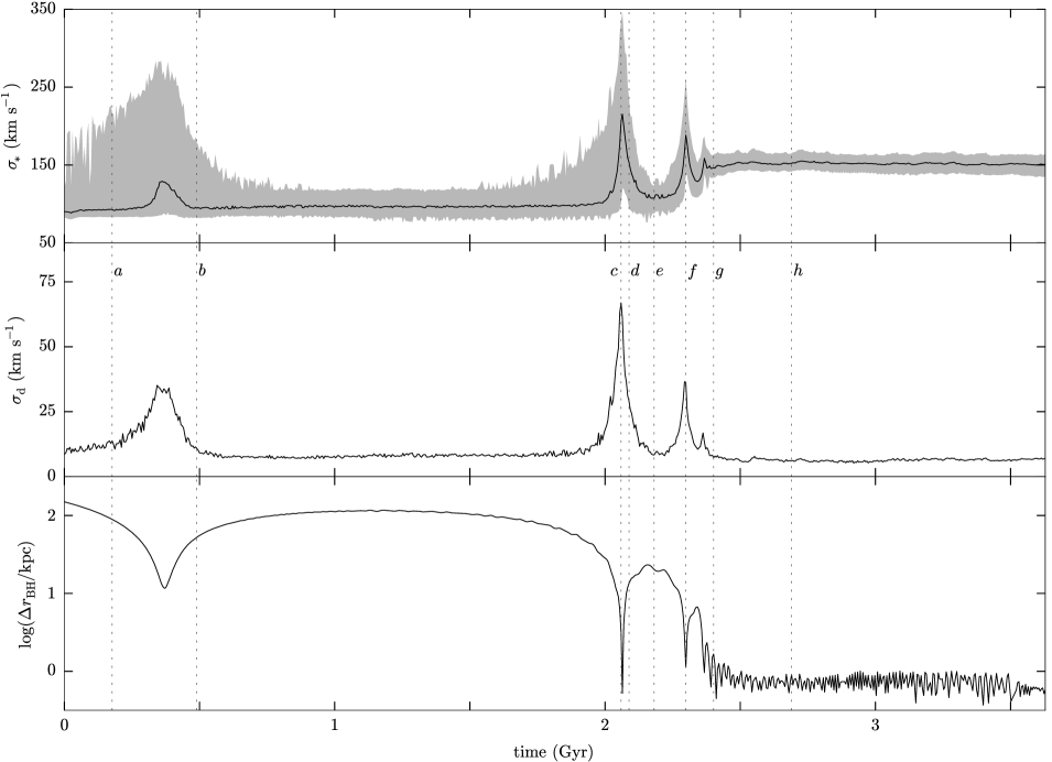
Figure 1.— Merger evolution time series for simulation S1. Upper panel: The mean value of $\sigma_{\!*}$ over the set of 1000 viewing directions is plotted in black. The upper and lower edges of the gray shaded region show the maximum and minimum values of $\sigma_{\!*}$. Middle panel: The standard deviation of the set of $\sigma_{\!*}$ measurements. Lower panel: The distance between the two SMBH particles. This is a proxy for the distance between the nuclei of the two progenitors. The dotted vertical lines indicate the time coordinates of snapshots that are examined in further detail later in this paper. Visual renderings of these snapshots are presented in Figure 2. The snapshots are located at $a=0.177$ Gyr, $b=0.490$ Gyr, $c=2.060$ Gyr, $d=2.089$ Gyr, $e=2.181$ Gyr, $f=2.299$ Gyr, $g=2.401$ Gyr, and $h=2.690$ Gyr.

The parent dark matter halos of the progenitors initially overlapped somewhat, however the stellar components were initially significantly separated. The progenitors followed approximately parabolic orbits while approaching one another. Tidal forces grew stronger and began to visibly elongate and warp the progenitors as they prepared to collide. Shortly before reaching their pericentric distance, the galaxies began to overlap significantly and $\sigma_{\!*}$ began increasing. Simultaneously, the standard deviation of the $\sigma_{\!*}$ distribution ($\sigma_{\rm d}$) increased. The gas components of the progenitors collided and became compressed. A small fraction of the gas lost enough angular momentum in this initial collision to begin migrating toward the nuclei of the progenitors. As the nuclei reached the pericentric distance, $\sigma_{\!*}$ reached a maximum value. This increase in $\sigma_{\!*}$ was primarily due to the projected streaming motion of the progenitors rather than a true increase in $\sigma_{\!*}$; lines of sight perpendicular to the collision axis experienced very little enhancement in $\sigma_{\!*}$, while lines of sight coinciding with the collision axis (i.e., lines of sight along which stars of both bulges simultaneously fell within the measuring slit) yielded the largest values of $\sigma_{\!*}$.

While receding from the first encounter, the velocity dispersion of each progenitor quickly returned to its pre-collision value. Strong tidal tails and a bridge of stars and gas began forming. A small amount of gas finally reached the nuclei and triggered short, sporadic episodes of AGN activity upon reaching the SMBHs. Gas in the tidal tails collapsed to form thin filaments as the galaxies continued to recede. The filaments then fragmented to form clumps from which clusters of stars soon formed as discussed in Elmegreen et at. (1993), Barnes & Hernquist (1996), Wetzstein et al. (2007), and references therein. The approximate time of the fragmentation and cluster formation in merger S1 is marked by snapshot b in Figure 1. These clusters, which can be seen in Figure 2 and Figure 3 as bright compact spots, most likely represent tidal dwarf galaxies. With diameters of 50–300 pc and masses of $10^{7}$–$10^{9}\,\rm M_{\sun}$, these systems lie near the resolution limit of our simulations; some of the smaller ones may merely indicate the formation sites of small structures such as globular clusters. Observational evidence for such tidal dwarf galaxies is reviewed in Dabringhausen & Kroupa (2013). Although no tidal dwarf systems formed in our dissipationless merger, we note that it is possible for tidal dwarf systems to form in dissipationless mergers at this stage (see Barnes, 1992, for details).

After receding from one another, the progenitors eventually reversed direction and began approaching one another on a trajectory that was much more nearly head-on than the first approach. Upon the second approach, the interstellar gas of the two progenitors collided once again (snapshot c), losing considerably more angular momentum this time. In contrast with the first encounter, $\sigma_{\!*}$ increased along all lines of sight; the minimum, maximum, mean, and standard deviation of $\sigma_{\!*}$ increased sharply as the nuclei passed through one another and then decreased as the nuclei receded (see snapshots d and e). As the nuclei reversed direction again, $\sigma_{\!*}$ nearly returned to its initial value. Simultaneously, in-falling clumps of low-angular momentum gas began reaching the central SMBHs, triggering significant episodes of AGN activity. The nuclei then began approaching one another while stars in the outer regions of the merging system, where the dynamical timescale was longer and the stars were less tightly bound, continued on nearly the same trajectories that they followed during the second approach—essentially unaffected by the motion of the nuclei.

As the nuclei began to overlap for the third time, AGN activity decreased significantly and $\sigma_{\!*}$ increased once again (snapshot f). After passing through one another once more, the velocity dispersion of each nucleus decreased somewhat, but it did not return to its initial value. This process was repeated several more times in rapid succession, with more stars being shed from the nuclei during each reversal. The nuclear turnaround distance decayed until the two nuclei eventually coalesced (at snapshot g). Oscillations in the value of $\sigma_{\!*}$ decayed away during this stage and the system adopted a new, stable $\sigma_{\!*}$. During the final stages of nuclear coalescence, gas and stars of low angular momentum began falling into the deep potential well of the new nucleus. This triggered a nuclear starburst which was soon followed by the highest SMBH accretion rates of the entire merger process. The accretion episodes during this stage were more frequent and more sustained than at any other time during the simulations (see images of snapshot g for the corresponding morphology). The surrounding gas became heated by the AGN, expanded, and drove significant gas outflows (see Hopkins et al., 2006, for a detailed discussion of these phenomena). The stars that fell toward the nucleus soon passed through the nucleus and emerged in spherical waves on the other side only to fall back onto the nucleus again. The effect of the stars falling toward the nucleus, overshooting, and then falling back caused small, statistically significant fluctuations in $\sigma_{\!*}$—the same oscillations that were observed in the “phase mixing” merger stage described in SC1. The amplitude of these oscillations gradually decreased as the system became more throughly mixed. Stars that were ejected after the second and third passes gradually fell back toward the nucleus during the $\approx 1$ Gyr following the final coalescence. In all of our dissipative simulations, clumps of gas that were ejected without being significantly heated earlier in the merger process also fell back toward the nucleus and formed a series of nuclear disks with diameters ranging from 100 pc to 10 kpc (disks smaller than 100 pc could not be resolved). The formation of similar disks is discussed in Barnes (2002). Gas of sufficiently low angular momentum was able to accrete onto the SMBH(s), causing another period of significant AGN activity $\gtrsim 1$ Gyr after final coalescence. This late-stage accretion was observed in all of our mergers except for the lowest gas mass fraction mergers, S0 and S6. In mergers that still contained two distinct SMBHs at this late stage, the formation of the nuclear disks allowed for efficient angular momentum transfer from the SMBHs to the disk material, as discussed in Gould & Rix (2000) and Escala et al. (2005). In real galaxies, the SMBHs have most likely merged before this late stage; the spatial resolution of our simulations was insufficient to follow the details of the binary SMBH orbital decay (Escala et al., 2005), thus the SMBH merger timescale could not be accurately simulated. Images of the final remnant galaxies are presented in Figure 3.

3.2. Dependence upon Initial Parameters

The general shapes of the three time series shown in Figure 1 are shared by all of our mergers—including the dissipationless merger, S0. Rather than presenting plots for each merger, we have summarized the basic features of each merger in Table 3. We report the time coordinates of the first three passes ($t_{1}$–$t_{3}$), the mean stellar velocity dispersion of the systems during each pass ($\sigma_{1}$–$\sigma_{3}$), the time at which the nuclei coalesced ($t_{\rm nc}$), the value of $\sigma_{\!*}$ in the remnant, and the duration of each simulation.

Simulations S1, S2, and S3 tested the dependence of $\sigma_{\!*}$ upon the spin-orbit configuration of the initial system. From the data, it appears that configurations of lower net angular momentum cause more significant increases in $\sigma_{\!*}$ during the first encounter; the high angular momentum, prograde-prograde merger (S1) exhibited the lowest $\sigma_{1}$ value, while the merger of lowest angular momentum (S3) exhibited the highest value of $\sigma_{1}$. No other trends were observed with respect to the spin-orbit configuration.

The gas fraction of the disk component was varied from 0.0 to 0.4 in simulations S0, S1, S6, and S7. The elapsed time between the first and second encounters was mildly dependent on the gas fraction, with higher gas fractions leading to shorter intervals. This was likely caused by the dissipative, collisional nature of the gas; when more gas was present, translational kinetic energy was more efficiently converted into internal energy, resulting in slightly lower recession velocities. The star formation rate was higher in mergers with larger gas fractions, since these systems contained more raw material from which to build stars. In Figure 3, we see that the number of tidal dwarf galaxies also increased with gas fraction. The presence of more dwarfs made the time series data slightly more noisy as the gas fraction increased from 0.1 to 0.4. However, note that the remnant of the completely dissipationless merger (i.e., the gas-free merger, S0) exhibited the least stable value of $\sigma_{\rm final}$, even though no tidal dwarf systems formed. This was apparently due to the phase mixing process, described in SC1, which was more pronounced in the absence of dissipation. We found no clear relationship between gas fraction and $\sigma_{\rm final}$.

In simulations S1, S4, and S5, the mass ratio of the progenitors was varied. Unsurprisingly, systems of comparable mass were able to disturb one another more effectively. This led to more significant enhancements in $\sigma_{\!*}$ during the merger process. The other trends evident in S1, S4, and S5 can be attributed to the varying total masses of these systems; the systems of higher total mass merged more rapidly and produced systems of higher $\sigma_{\!*}$.

In simulation S8, as well as many low-resolution trial simulations, the orbital parameters were varied. Smaller pericentric distances lead to faster mergers and larger enhancements in $\sigma_{\!*}$ during the first pass. In the case of nearly head-on initial encounters, $\sigma_{\!*}$ reaches its absolute highest value during the first pass rather than the second pass.

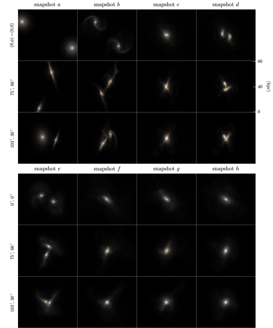
Figure 2.— Visualizations of snapshots from simulation S1, created using GSnap’s volume rendering algorithm. The snapshot times correspond to the dotted vertical lines in Figure 1. Each snapshot is shown from three directions, indicated in spherical coordinates on the left. The width and height of each image is 93.75 kpc and 81.19 kpc, respectively.

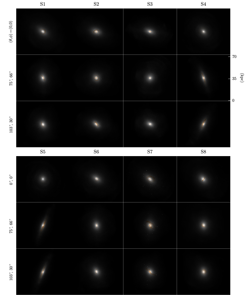
Figure 3.— The remnants of merger simulations S1–S8, listed in Table 2. The simulation time of each snapshot is listed in Table 3, as $t_{\rm end}$. Each remnant is viewed from the same three directions as the images in Figure 2. Each field of view measures 84.38 kpc $\times$  73.071 kpc. All remnants are elliptical except for S4 and S5—the unequal mass mergers. All systems contain nuclear disks.

3.3. The Distribution of $\sigma_{\!*}$

While the time series presented in Figure 1 are helpful for understanding the evolution of $\sigma_{\!*}$ with time, they do not contain much information regarding the distribution of $\sigma_{\!*}$ during the merger process. To supplement the time series data, we present, in Figure 4, the angular and probability distributions of $\sigma_{\!*}$ in four snapshots during merger S1. For each of these four snapshots, $\sigma_{\!*}$ was measured along 20,000 lines of sight.

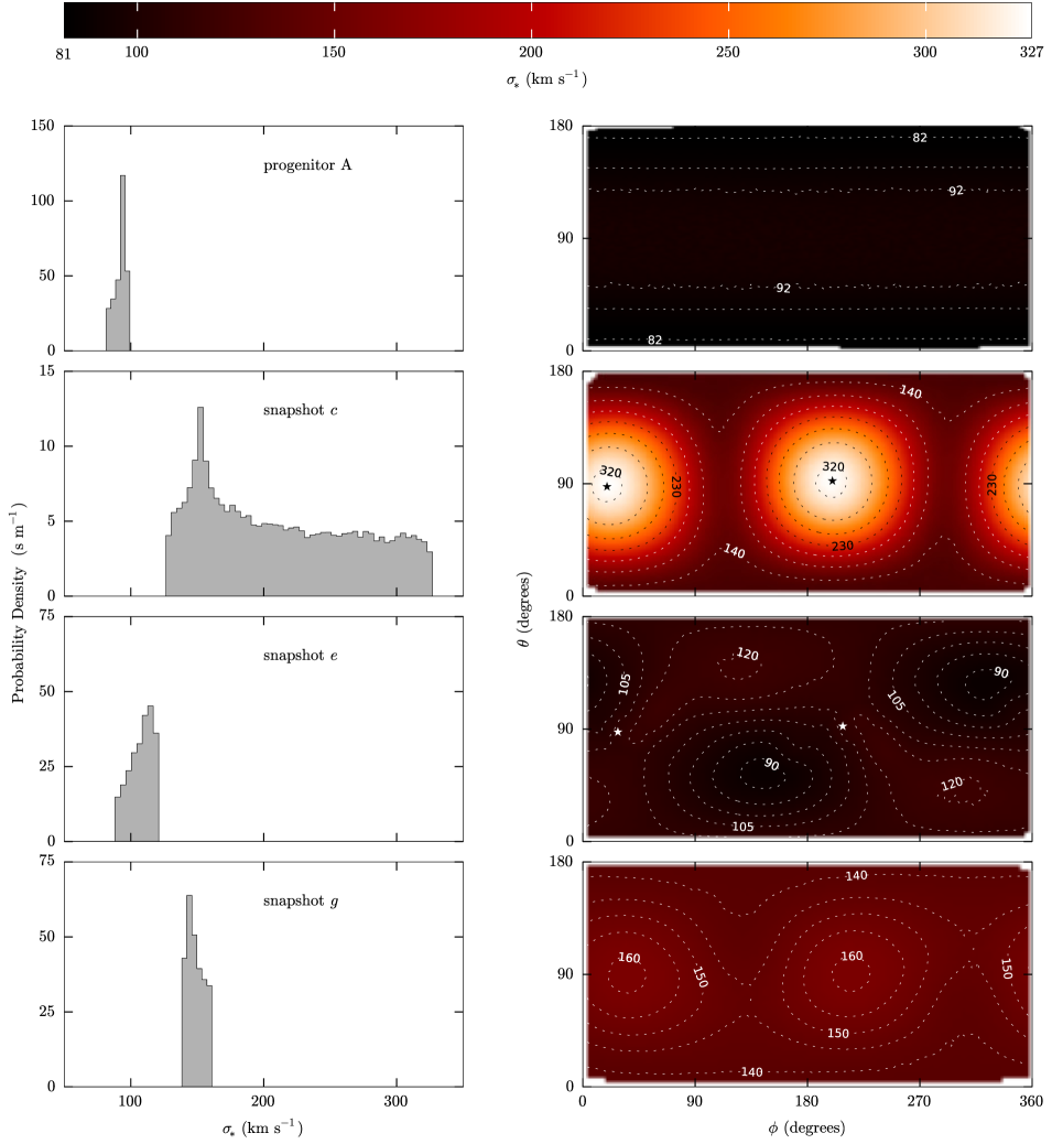
Figure 4.— The angular and probability distributions of $\sigma_{\!*}$ in progenitor galaxy A (upper panel), followed by snapshots c, e, and g of simulation S1 (see Figure 1 for more information on the meaning of these labels). For each snapshot, $\sigma_{\!*}$ was measured along 20,000 random directions. The contour plots on the right show the directional variation of $\sigma_{\!*}$, while the histograms on the left show the corresponding probability distributions. The star symbols indicate the directions that lie along the instantaneous collision axis, where applicable. For a discussion of this figure, see section 3.3.

In the progenitor galaxy, $\sigma_{\!*}$ is distributed nearly isotropically. The presence of a stellar disk is evident from the symmetry about the equator of the system ($\theta=90^{\circ}$). Measurements of $\sigma_{\!*}$ along lines of sight perpendicular to the disk are diminished by the presence of the disk stars while measurements made along the edge of the disk are enhanced somewhat because, from these sight lines, the disk’s rotation can contribute to the velocity dispersion measurements.

The second snapshot of interest (snapshot c) was recorded shortly before the climax of the second encounter. It shows that the highest values of $\sigma_{\!*}$ are measured along the collision axis (denoted by the star symbols) while the lowest values are measured perpendicular to the axis. Furthermore, the positive skew of the probability distribution indicates that a random measurement of $\sigma_{\!*}$ during a collision is more likely to yield a value near the mean or minimum rather than near the maximum possible value ($\sigma_{\!*,\rm max}$). The reason $\sigma_{\!*}$ is highest along the collision axis is twofold: (1) the two progenitors are moving with respect to each other along this axis; their combined bulk motion is mistaken for stellar velocity dispersion when the system is viewed along this direction, and (2) the actual velocity dispersion of each progenitor increases along the collision axis during collisions. These separate effects are discussed in more detail in the next section.

Midway between the second and third passes (snapshot e), the lines of sight yielding the maximum measurements of $\sigma_{\!*}$ no longer coincide with the instantaneous collision axis. We can also see that a random measurement of $\sigma_{\!*}$ is more likely to fall near the maximum value than near the minimum. However, the system is considerably more isotropic than it was during the climax of the second pass, so the difference between the minimum and maximum values of $\sigma_{\!*}$ is much less significant here.

Immediately after nuclear coalescence (snapshot g), $\sigma_{\!*}$ is already distributed quite uniformly; the difference between the maximum and minimum $\sigma_{\!*}$ is much smaller than during snapshot c. The contours in the angular distribution plot for snapshot g indicate that the velocity dispersion is highest along a preferred axis—similar to the distribution in snapshot c. This axis corresponds to the collision axis during the last few encounters before coalescence, which is not necessarily the same as the collision axis during the second pass.

3.4. Random versus Streaming Motion

The measurements of $\sigma_{\!*}$, discussed above, have been based upon a straightforward application of Eq. (2) to all stars appearing in a slit mask centered on one of the nuclei of a merging system. Since this is the observationally accessible quantity, it would be more appropriate to refer to this version of $\sigma_{\!*}$ as the apparent velocity dispersion. The apparent velocity dispersion includes the effects of rotation and bulk motion whereas the intrinsic velocity dispersion is due to the purely random motion of stars in the system.

Suppose two systems with intrinsic velocity dispersions $\sigma_{1}$ and $\sigma_{2}$ move toward or away from one another with speed $v$. Let $m_{1}$ and $m_{2}$ be the portions of the stellar masses of systems 1 and 2 that appear within a slit. Using Eq. (2), it is possible to show that the apparent velocity dispersion along the line of sight connecting the centers of two systems is given by,

$$\sigma_{\!*}=\sqrt{f_{1}\sigma_{1}^{2}+f_{2}\sigma_{2}^{2}+f_{1}f_{2}v^{2}},$$ (3)

where $f_{i}$ are the fractional masses,

$$f_{i}=\frac{m_{i}}{m_{1}+m_{2}}.$$

For the special case of two identical systems of velocity dispersion $\sigma_{0}$ on a collision course, a measurement of $\sigma_{\!*}$ along the collision axis will yield

$$\sigma_{\!*}=\sqrt{\sigma_{0}^{2}+(v/2)^{2}},$$ (4)

since $m_{1}=m_{2}$ and $\sigma_{1}=\sigma_{2}=\sigma_{0}$.

In major mergers, the $\sigma_{\!*}$ appearing on the left side of Equations (3) and (4) typically corresponds to the maximum measurement of velocity dispersion in the merging system. Thus, $\sigma_{\!*,\rm max}$ can be used as an approximation for this quantity. The relative radial speed of the two systems, $v$, can be approximated using the relative radial speed of the two SMBHs. More precisely, if $\mathbf{r}$ is a position vector pointing from one black hole to the other and $\mathbf{v}$ is the corresponding relative velocity vector, the speed $v$ is given by $v=|\hat{\mathbf{r}}\cdot\mathbf{v}|$, where $\hat{\mathbf{r}}=\mathbf{r}/|\mathbf{r}|$.

Figure 5.— Separating the intrinsic and apparent velocity dispersions. Upper panel: The solid black line shows $v/2$, defined in Section 3.4. The gray dashed line shows the maximum apparent velocity dispersion ($\sigma_{\!*{\rm,max}}$) as a function of time during merger S1. Both quantities have been smoothed over time to remove high frequency fluctuations. Lower panel: The solid line shows the intrinsic velocity dispersion, $\sigma_{0}$, discussed in Section 3.4. The dashed line shows the mean value of $\sigma_{\!*}$  over the set of 1000 viewing directions; it is a smoothed version of the plot in the upper panel of Figure 1. Note that the mean velocity dispersion closely traces the intrinsic velocity dispersion.

In the special case of a merger of identical systems, measuring $\sigma_{\!*,\rm max}$ and $v$ allows us to infer the intrinsic velocity dispersion ($\sigma_{0}$) of each system, using Equation (4). In Figure 5, we show the result of decomposing measurements of apparent velocity dispersion into streaming and intrinsic components. The analysis was performed on merger S1, which began as a merger of identical systems. The upper panel shows $\sigma_{\!*,\rm max}$ and $v/2$ while the lower panel shows the intrinsic velocity dispersion, $\sigma_{0}$, measured along the collision axis. The results suggest that the mean of $\sigma_{\!*}$ over all directions (the dashed line in the lower panel) closely traces the intrinsic velocity dispersion (the solid line). The intrinsic velocity dispersion along the collision axis is only mildly elevated in comparison with the mean value of $\sigma_{\!*}$. However, there are several caveats: First, we note that the velocity of a SMBH does not trace the velocity of its parent nucleus perfectly. In general, each SMBH particle orbits the center of its parent nucleus. We have smoothed the $v$ time series in order to remove high frequency variations caused by this motion. For consistency, we also smoothed the $\sigma_{\!*,\rm max}$ time series. Secondly, the velocity of a nucleus does not always trace the bulk velocity of its parent progenitor galaxy. In fact, neither progenitor galaxy has a well-defined bulk velocity during a collision; as the progenitor systems become increasingly superimposed, the streaming velocity in each progenitor begins to vary with position. Finally, even though $\sigma_{\!*,\rm max}$ is usually a good approximation for the quantity on the left side of Equation (4), this is not necessarily true at the turnaround times when the streaming velocity is low. In such cases, the maximum velocity dispersion is not necessarily measured along the collision axis (see Figure 4). In light of these complexities, it would be best to interpret the resulting plot of $\sigma_{0}$ qualitatively rather than quantitatively.

3.5. Evolution with Stellar Age

It has long been known that the velocity dispersion of stars in the disk of the Milky Way increases with age. This so-called “age-velocity relation,” along with the phenomena which cause it, have been studied for more than six decades (Spitzer & Schwarzschild, 1951, 1953; Barbanis & Woltjer, 1967; Hänninen & Flynn, 2002; Nordström et al., 2004). More recently, it has been shown that measurements of $\sigma_{\!*}$ in more distant galaxies can depend upon the population of stars being measured (Rothberg & Fischer, 2010; Rothberg et al., 2013). Specifically, measurements of $\sigma_{\!*}$ that are based upon the spectral features of younger stars yield lower values than measurements of $\sigma_{\!*}$ which include all stars or only older K and M stars. To explain this “$\sigma$-discrepancy,” Rothberg et al. argue that stars are born with low velocity dispersion, since the gas from which stars form is dynamically cold, due to its dissipative, collisional nature.

In order to investigate whether our simulations exhibited age-dependent $\sigma_{\!*}$, we performed the analysis described in sections 2.1.2 and 2.1.3 using only stars in specified age ranges. Before presenting our findings, though, we note that the results presented in this section necessarily depend strongly upon the less robust aspects of the simulation code—namely, the numerical methods used to simulate the hydrodynamics, star formation, and SMBH feedback. These methods effect the timing, location, and rate of the star formation. Furthermore, the particles traced by our simulations do not represent individual stars. Instead, they represent small regions of star formation. This means that cluster evaporation and other small-scale effects are not included. Therefore, our results regarding the evolution of $\sigma_{\!*}$ with stellar age are less robust than our age-independent analysis.

In Figure 6, we present the evolution of $\sigma_{\!*}$ for stars in three age bins during simulation S1 by plotting the offset from the instantaneous global value of $\sigma_{\!*}$ (i.e., the value of $\sigma_{\!*}$ based on stars of all ages). The star formation rate is plotted in the same figure for reference.

Stars that formed during the first 0.5 Gyr of the simulation were located in the disks of the progenitor systems. These stars were born with $\sigma_{\!*}\approx 12\rm\,km\,s^{-1}$ lower than the global velocity dispersions of their parent galaxies. Immediately after the first pass, the offset was a mere $\approx 7\,\rm km\,s^{-1}$. These stars gradually mixed and became dynamically heated. By the end of the simulation, they were essentially dynamically indistinguishable from the system as a whole.

Figure 6.— The evolution of $\sigma_{\!*}$ for various stellar age bins. Upper panel: The star formation rate in simulation S1. Lower panel: The offset from the global, mean velocity dispersion that includes stars of all ages, $\Delta\sigma_{\!*}=\sigma_{\!*}-\sigma_{\!*,\rm all}$ for three stellar age bins of width 0.5 Gyr. Each line is labeled with its age bin. For example, the top line shows the evolution of $\Delta\sigma_{\!*}$ for all stars that were born between time $t=0$ Gyr and $t=0.5$ Gyr. The vertical dashed lines indicate snapshot times introduced in Figure 1.

The evolution of stars that formed between 1.0 Gyr and 1.5 Gyr (i.e., between the first and second passes) after the beginning of the simulation was more complicated because approximately 70% of these stars formed in tightly-bound tidal tidal dwarf-like systems. The dwarf galaxies repeatedly passed near the nuclei of the larger systems. This lead to large fluctuations in the $\sigma_{\!*}$ evolution time series. While the two primary galaxies were approaching one another, in preparation for their second encounter, $\sigma_{\!*}$ in this age bin generally increased. However, after the second pass, $\sigma_{\!*}$ began decreasing; the offset from the global $\sigma_{\!*}$ increased while the global value remained essentially constant, as seen in Figure 1. This behavior is due to the orbital decay of the satellite galaxies in which these stars are primarily located.

Finally, stars that were born between 2.5 Gyr and 3.0 Gyr (i.e., immediately following nuclear coalescence) formed exclusively in the nuclear disks and satellite galaxies (in the case of simulation S1, 85% formed in the nuclear disks while the remaining 15% formed in the satellite galaxies). The behavior of $\sigma_{\!*}$ in this group was similar to the 1.0 Gyr to 1.5 Gyr group, although the offset was larger by $\approx 10\rm\,km\,s^{-1}$.

Figure 7.— The relation between $\sigma_{\!*}$ and stellar age in simulation S1. The snapshot examined here was saved at 3.5 Gyr (i.e., stars that formed at $t=0$ Gyr are 3.5 Gyr old). The vertical dashed lines indicate the ages of stars that were born at the corresponding snapshot times shown in Figures 1 and 6. The horizontal bar indicates the global value of $\sigma_{\!*}$ in the current snapshot.

In Figure 7, we have plotted $\sigma_{\!*}$ as a function of stellar age in the remnant system in a simulation snapshot that was saved at $t=3.5$ Gyr. From this, it is clear that younger stars tend to have lower $\sigma_{\!*}$ than older stars, but there are complexities; the history of the merger has been imprinted onto the dynamics of the remnant. The stars that formed before the first pass (i.e., the stars older than $3.0$ Gyr) have had time to become dynamically heated. As we saw in Figure 6, these stars were initially rapidly heated during the first pass and then gradually heated during the remainder of the merger. Stars that formed immediately after the first pass have had fewer opportunities to become mixed and heated. As mentioned in the discussion of Figure 6, many of these stars formed in tidal dwarf galaxies that underwent a decrease in $\sigma_{\!*}$ after the second pass. Consequently, the oldest of these stars have the lowest value of $\sigma_{\!*}$, so the slope of the relation is inverted for stars between 1.7 Gyr and 2.7 Gyr old. Stars that formed during and after the second pass have had even fewer opportunities to become dynamically heated. All of the stars that were born during the second starburst (indicated by the vertical dashed line labeled g) formed either in the nuclear cluster of the newly-coalesced system or the satellite galaxies, with the majority forming in the nuclear cluster. These stars cooled dynamically over time as the orbits of the satellite galaxies decayed. Finally, the majority (85%) of the stars with ages less than 0.5 Gyr, formed in nuclear disks with very low velocity dispersion and have not had time to become substantially heated.

4. ADDITIONAL STATISTICS

4.1. AGN Activity

Observations examining the cosmic evolution of the $M_{\rm BH}$–$\sigma_{\!*}$ relation (e.g., Treu et al., 2004, 2007; Woo et al., 2006, 2008; Hiner et al., 2012; Canalizo et al., 2012) appear to indicate that SMBHs formed more rapidly than their host galaxies; given a fixed value of $\sigma_{\!*}$, galaxies at redshifts of $z>0.1$ have more massive black holes than local galaxies. Unfortunately, in order to measure $M_{\rm BH}$ in non-local galaxies, a SMBH must be actively accreting gas. Exclusively using AGN host galaxies in such studies raises the concern that the sample may be biased in various ways. For example, AGNs are often associated with galaxy merger activity (e.g., Canalizo & Stockton, 2013, and references therein). Depending on the timing of the AGN activity with respect to the merger activity, measuring $\sigma_{\!*}$ in AGN hosts galaxies could introduce extra scatter in the resulting $M_{\rm BH}$–$\sigma_{\!*}$ relation or it could systematically bias the value of $\sigma_{\!*}$ to higher or lower values, leading to an artificial offset.

In order to determine whether $\sigma_{\!*}$ differs statistically between AGN host galaxies and inactive galaxies, we examined the dynamical circumstances under which significant accretion occurred during each of our simulations. The characteristic SMBH accretion timescale in our simulations was shorter than, or comparable to, our resolution limit of 5 Myr; the accretion rate frequently changed by factors of 10–100 between consecutive snapshots. Consequently, we likely did not capture all of the enhanced accretion activity. Nevertheless, by examining all of our simulations, we were able to clearly identify periods during which significant accretion was likely to occur as well as periods during which significant accretion was not likely. For a detailed discussion of AGN lifetimes in hydrodynamic simulations similar to ours, as well as a summary of observational evidence, see Hopkins et al. (2006), Hopkins & Hernquist (2009) and references therein. We found that accretion corresponding to a bolometric luminosity of $10^{44}\,\rm erg\,s^{-1}$ appeared to be a natural threshold separating the most luminous AGN activity from the much more frequent periods of less significant accretion. Incidentally, $10^{44}\,\rm erg\,s^{-1}$ is also commonly adopted as the threshold separating quasars and Seyfert galaxies, so we use the phrases “significant accretion” and “quasar-level accretion” interchangeably.

All significant (quasar-level) accretion occurred during four periods. In Figure 8, these periods are shown with gray shading along with generic merger time series plots of $\sigma_{\!*}$, star formation rate, and black hole separation. Period I occurred shortly after the first pass while the progenitors were receding from one another. Period II occurred between the second and third passes. Both progenitors hosted quasars during these periods, but usually not simultaneously; the quasars turned on and off independently of one another, as discussed in more detail by Van Wassenhove et al. (2012). This suggests that binary quasars with separations of 10–100 kpc are rare, relative to the occurrence of quasars in general. Period III began at the moment of nuclear coalescence and period IV occurred long after coalescence, when some of the gas that was not significantly heated during period III fell toward the nucleus. Periods III and IV were associated with the most luminous quasars observed during our mergers, with $L_{\rm bol}\sim 10^{45}\,\rm erg\,s^{-1}$. Interestingly, quasar-level accretion was never observed during the second or third passes when the velocity dispersion was substantially elevated. This may be due to the $v_{\infty}$ term in the denominator of Equation (1), since the relative speed of the SMBH with respect to the surrounding gas tends to increase during the collisions. Accretion corresponding to bolometric luminosities of $L_{\rm bol}<10^{44}\,\rm erg\,s^{-1}$ occurred sporadically at all times after the first pass—including the second and third passes. We note that quasar-level accretion did not occur during all four periods in each simulation, however when quasar-level accretion was detected, it was always during one (or more) of the four periods identified in Figure 8. While this does not imply that quasar-level accretion never happens during other stages of the merger, it suggests that quasar activity is rare during other stages of merger evolution.

Figure 8.— Periods of significant accretion during a generic merger. All significant accretion (with $L_{\rm bol}\gtrsim 10^{44}\,\rm erg\,s^{-1}$) occurred during one of four periods: (I) Shortly after the first pass, (II) between the second and third passes, (III) during and immediately following nuclear coalescence, and (IV) long after nuclear coalescence. Not all mergers exhibited significant SMBH accretion during all four periods.

For each simulation, the mean offset of $\sigma_{\!*}$ from the fiducial value was computed during each of the four quasar periods. There was no detectable offset in $\sigma_{\!*}$ during periods I, III, and IV, however an offset was always present during period II. Since the fiducial value of $\sigma_{\!*}$ during period II is somewhat ambiguous, we computed two mean fractional offsets: the offset from the progenitor system, $(\sigma_{\!*}-\sigma_{\rm prog})/\sigma_{\rm prog}=0.11\pm 0.05$, and the offset from the final remnant system, $(\sigma_{\!*}-\sigma_{\rm final})/\sigma_{\rm final}=-0.28\pm 0.02$. Due to these offsets, the inclusion of period II quasar host galaxies in an observational sample could potentially introduce extra scatter, or an offset, in a plot of the $M_{\rm BH}$–$\sigma_{\!*}$ relation. In Figure 8, we see that the SMBHs are significantly separated during period II. Therefore, a measurement of $M_{\rm BH}$ in such a system would correspond with the mass of a progenitor SMBH. The fiducial value of $\sigma_{\!*}$ used in the $M_{\rm BH}$–$\sigma_{\!*}$ relation would then be the pre-merger value of the progenitor spheroid. If we assume that progenitor systems generally fall within the scatter of the local $M_{\rm BH}$–$\sigma_{\!*}$ relation, then observations of period II systems would tend to have high values of $\sigma_{\!*}$ relative to their $M_{\rm BH}$. Stated differently, these systems would appear to have under-massive black holes when placed on the $M_{\rm BH}$–$\sigma_{\!*}$ diagram. Thus, the overly massive black holes that are observed at high redshift cannot be due to measurements of period II systems. Furthermore, in our simulations, period II quasar activity accounted for only 16.1% of all quasar-level AGN activity; it is unlikely that a large fraction of randomly selected quasar hosts would consist of period II systems. Finally, from the images of the period II system (snapshot e) in Figure 2, it is evident that period II systems are composed of two distinguishable galaxies (when viewed along most lines of sight), so they should be relatively easy to identify.

When interpreting these results, one should be aware that the timing of quasar activity depends upon the treatment of hydrodynamics and SMBH feedback in our simulations. We have tried to make our results more robust by considering only the general periods of likely accretion, rather than the exact timing of the accretion. However, recent work by Hayward et al. (2013) suggests that the hydrodynamic evolution in the late stages of GADGET-3 simulations can differ significantly from the evolution observed in more realistic simulations when SMBH feedback is included. This casts some doubt on the timing and prevalence of Period IV quasars, but our general finding remains unchanged; during a period of quasar activity, $\sigma_{\!*}$ is not likely to be strongly offset from its fiducial value. Even if Period IV quasars never occur in nature, the majority of quasar activity still occurs during periods when $\sigma_{\!*}$ is not significantly offset. Alternatively, if Period IV accretion is more likely in reality than our simulations suggest, then observing a quasar host with an elevated velocity dispersion would be more rare than our simulations suggest, since Period IV quasars occur after the $\sigma_{\!*}$ has reached a stable value.

4.2. Intrinsic Scatter

Measurements of $\sigma_{\!*}$ in real galaxies are necessarily made from random viewing directions at random times during galactic evolution. There is no way of observationally determining the intrinsic scatter of $\sigma_{\!*}$ with respect to its quiescent, fiducial value. Using our simulation data, we are able to provide estimates of this intrinsic scatter. Since observed systems can broadly be categorized as either ongoing mergers or passively evolving (or simply “passive”) systems, we present two intrinsic scatter estimates—one for passive systems and one for ongoing mergers. In this analysis, three conditions must be met for a galaxy to be considered passive:

1. The galaxy must be clearly distinguishable from neighboring galaxies.

2. The galaxy must contain only one nucleus.

3. The galaxy must contain at most one large disk structure.

If any of these general criteria are not met, then the system is considered an ongoing merger. Passive systems include all systems that appear to be non-interacting as well as systems that have clearly undergone recent interactions. For example, even though the progenitors in simulation S1 show strong signs of interaction after the first pass (see snapshot b in Figure 2), we classify them as passive galaxies between approximately 0.5 Gyr and 2.0 Gyr. The system is also classified as passive immediately after nuclear coalescence, at 2.4 Gyr, even though there are signs of recent interaction, such as stellar shells (see snapshots g and h). We classify simulation S1 as an ongoing merger between 2.0 Gyr and 2.4 Gyr (snapshots c–f) and also during the first pass, between approximately 0.25 Gyr and 0.4 Gyr. Admittedly, there are special circumstances that can cause an ongoing merger to appear to be a passive system and vice versa. In the present paper, we have ignored these effects.

Figure 9.— Scatter probability distribution for coalesced systems, where $\Delta\sigma_{\!*}$ is the offset from the mean value of stellar velocity dispersion, $\langle\sigma_{\!*}\rangle$. This plot includes data from all snapshots from simulations S1–S8) saved during periods of passive evolution, as defined in section 4.2. The best-fitting Gaussian, with $\sigma=0.042$ and $\mu=1.25\times 10^{-5}$ is over-plotted.

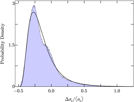
Figure 10.— Scatter probability distribution for merging systems, where $\Delta\sigma_{\!*}$ is the offset from the mean value of stellar velocity dispersion of the final remnant, $\langle\sigma_{\!*}\rangle=\sigma_{\rm final}$. This plot includes data from all snapshots from simulations S1–S8 saved between the onset of the second pass and nuclear coalescence. The best-fitting log-normal distribution, with $\sigma=0.543$, $\mu=-1.150$, and $\delta=-0.509$, is over-plotted.

Upon separating each merger simulation into periods of ongoing merger activity and periods of passive evolution, we computed the probability distribution of the fractional offset, $\Delta\sigma_{\!*}/\langle\sigma_{\!*}\rangle$ from the fiducial value. The quantity $\Delta\sigma_{\!*}=\sigma_{\!*}-\langle\sigma_{\!*}\rangle$ is the offset from the current fiducial value, $\langle\sigma_{\!*}\rangle$. In the passive period after the first pass, the fiducial value is the time average of the mean $\sigma_{\!*}$ time series during that period. In all other cases, the fiducial value is the time average of the mean $\sigma_{\!*}$ time series in the remnant system, $\sigma_{\rm final}$. In Figure 9, we present the probability distribution for passive systems. This plot contains data from all of our simulations. The best fitting elementary distribution (in the least squares sense) was the Gaussian,

$$\frac{dP}{ds}=\frac{1}{\sigma\sqrt{2\pi}}\exp\left[{-\frac{(s-\mu)^{2}}{2\sigma^{2}}}\right]$$ (5)

with $\sigma=0.042$ and $\mu=1.25\times 10^{-5}$. The corresponding plot for ongoing mergers is presented in Figure 10. The best fitting elementary distribution in this case was the shifted log-normal distribution,

$$\frac{dP}{ds}=\frac{1}{\sigma\sqrt{2\pi}(s-\delta)}\exp\left[{-\frac{[\ln(s-\delta)-\mu]^{2}}{2\sigma^{2}}}\right]$$ (6)

with $\sigma=0.543$, $\mu=-1.150$, and $\delta=-0.509$. In both cases, the distribution is more closely fit by a linear combination of Gaussians; the above approximations are presented for simplicity. Using these densities, we can easily compute various probabilities. For example, in the absence of measurement error, the probabilities of measuring $\sigma_{\!*}$ within 5% of the fiducial value (i.e., $\sigma_{\rm final}$) are, respectively, 0.77 and 0.10 for passive systems and ongoing mergers. Furthermore, the probability of measuring $\sigma_{\!*}$ lower than the fiducial value ($\sigma_{\rm final}$) in an ongoing merger is 0.81.

While our approximation for the intrinsic scatter in passively evolving systems is likely fairly robust, the approximation for ongoing mergers likely depends more heavily upon our merger parameters. Given the characteristic directional distribution of $\sigma_{\!*}$ during a merger (see Figure 4) and the temporal evolution (see Figure 1), it is clear that the distribution is strongly skewed, like the log-normal distribution presented above. However, a greater variety of mergers would need to be examined in order to confidently compute the parameters of the distribution in ongoing mergers.

5. DISCUSSION AND CONCLUSIONS

In this paper, we have expanded upon the work presented in our previous paper (SC1) by examining the evolution of stellar velocity dispersion in a suite of eight binary disk galaxy merger simulations that included dissipation, dark matter, star formation, and AGN feedback. The analysis was designed, in part, to provide insight into observations of $\sigma_{\!*}$ in systems that show signs of recent or ongoing merger activity. Our primary findings are as follows:

1. During each merger, before the galactic nuclei coalesced, $\sigma_{\!*}$ underwent large, damped oscillations of increasing frequency. Once the nuclei coalesced, a series of small, statistically significant fluctuations continued until the remnant system became sufficiently mixed. Qualitatively, this behavior is consistent with the findings of SC1, which examined the evolution of $\sigma_{\!*}$ in more idealized mergers of spherically symmetric, dissipationless systems that did not contain a separate dark matter component.

2. Varying the gas fraction, and orbital parameters had no effect on the characteristic shape of the $\sigma_{\!*}$ evolution time series. The level of apparent noise in the time series depended upon the gas fraction in a non-trivial way. Systems with larger gas fractions tended to spawn more tidal dwarf systems. These dwarf systems added noise to the $\sigma_{\!*}$ time series because, while passing through the central region of their parent galaxy, they caused $\sigma_{\!*}$  to briefly increase. However, the presence of dissipation and star formation evidently caused the phase-mixing stage of the merger process to be less pronounced; $\sigma_{\!*}$ oscillated more significantly during the phase-mixing stage of the dissipationless merger than in any of the dissipative mergers.

3. No clear dependence was observed between the final velocity dispersion of the remnant and the gas fraction of the progenitors. However, $\sigma_{\rm final}$ was clearly lower in the completely dissipationless merger (S0) than in its dissipative counterparts (S1, S6, and S7). This is not surprising, since the dissipative merger remnants contained nuclear clusters of stars that formed during the simulation. The presence of a nuclear cluster deepened the gravitational potential well, leading to a larger $\sigma_{\!*}$. In the absence of AGN and stellar feedback, even more mass would have likely accumulated in the nuclear region, causing $\sigma_{\rm final}$ to be even higher. We could not test this quantitatively because running simulations without feedback was prohibitively expensive, due to the formation of many dense clumps of gas and stars.

4. Mergers of larger mass ratio (i.e., major mergers) exhibited the most significant absolute fluctuations in $\sigma_{\!*}$. However, the relative size of the fluctuations was not sensitive to the mass ratio. To see this, refer to the data from simulations S1, S4, and S5 in Table 3. These were, respectively, 1:1, 1:2, and 1:4 mergers with otherwise identical initial parameters. The value of $\sigma_{\!*}$ at the climax of the second pass ($\sigma_{2}$), was highest in S1 and lowest in S5, however, there was no trend in the fractional increase, $\sigma_{2}/\sigma_{\rm final}$.

5. When $\sigma_{\!*}$ is measured in systems that contain two progenitors moving relative to one another along the line of sight, the resulting measurements are artificially elevated because the streaming motion of the progenitors is mistaken for velocity dispersion. Equation 3 relates the apparent velocity dispersion of the combined system with the relative line-of-sight velocity and instrinsic properties of the progenitor systems.

6. During galaxy collisions, $\sigma_{\!*}$ increases in all directions. The enhancement in $\sigma_{\!*}$ is greatest along the collision axis, partially because the bulk motion of the two progenitor systems can be mistaken for true velocity dispersion, as noted above. Conversely, the enhancement is lowest along lines of sight perpendicular to the collision axis. The mean of $\sigma_{\!*}$ over the set of all possible viewing directions closely traces the intrinsic velocity dispersion of the system.

7. Stars in our simulations were born with lower $\sigma_{\!*}$ than that of the system as a whole. The apparent velocity dispersion of the youngest stars in the nuclear disks of our remnant systems was lower than the global stellar velocity dispersion by an average of $\approx 30~{}\rm km~{}s^{-1}$. New stars tended to become dynamically heated with time unless they were tightly bound into clusters or dwarf galaxies. The velocity dispersion of stars residing in dwarf galaxies decreased with respect to the global system as the orbits of their parent systems decayed due to dynamical friction.

8. Quasar-level accretion activity was not detected during times when $\sigma_{\!*}$ was strongly enhanced. On the other hand, Seyfert-level accretion occurred sporadically at all times after the first pass. In general, AGN activity does not preferentially occur when $\sigma_{\!*}$ is strongly offset from its fiducial, equilibrium value. This is consistent with recent observational evidence (Woo et al., 2013), indicating that active galaxies fall on the same $M_{\rm BH}$–$\sigma_{\!*}$ relation as quiescent galaxies.

Given our findings, we would advise anyone who is interested in measuring $\sigma_{\!*}$ in a dynamically questionable system to note the following:

• When $\sigma_{\!*}$ is measured in systems which clearly contain two nuclei, the resulting value of $\sigma_{\!*}$ in the individual nuclei depends upon the nuclear separation distance. Nuclei that are significantly separated (e.g., snapshot e in Figure 2) are likely to retain a value of $\sigma_{\!*}$ that is only slightly elevated with respect to the pre-collision value of the progenitor (compare the histograms for progenitor A and snapshot e in Figure 4). As the distance between the nuclei decreases, $\sigma_{\!*}$ increases. When the nuclei are strongly superposed, as in snapshot c, the measured value of $\sigma_{\!*}$ is likely to be higher than the value of $\sigma_{\!*}$ in the eventual remnant system. Of course, projection can also cause significantly separated nuclei to appear to be significantly superposed, so significant nuclear superposition is a weak diagnostic.

• A measurement of $\sigma_{\!*}$ is likely to be elevated relative to the eventual remnant value if the system contains two or more disk-like structures, but only one visible nucleus, as seen in snapshot c of Figure 2 (viewed along the $\theta=75^{\circ},\,\phi=66^{\circ}$ direction).

• Measurements of $\sigma_{\!*}$ in systems that contain only one nucleus are likely robust if the system also contains stellar shells or exhibits a dynamically relaxed morphology (see snapshot h). Shells tend to form after $\sigma_{\!*}$ has reached its stable post-merger value. More generally, if a system appears to be dynamically relaxed, a measurement of $\sigma_{\!*}$ is likely robust; the presence of low-surface brightness debris in the region surrounding a galaxy that otherwise appears to be relaxed does not indicate that $\sigma_{\!*}$ is enhanced.

• Measurements of $\sigma_{\!*}$ in the bulge components of disk-like systems containing strong bridges or tidal tails (e.g., snapshot b) are not likely to differ from the value of $\sigma_{\!*}$ measured in the bulge before the interaction took place.

• Systems with quasar-level luminosities ($L_{\rm bol}\gtrsim 10^{44}\,\rm erg\,s^{-1}$) are unlikely to have substantially elevated or suppressed values of $\sigma_{\!*}$, relative to the fiducial, equilibrium value.

For a concrete example, consider the prototypical ongoing merger, NGC 6240. This system contains two nuclei with a projected separation of $\sim 800$ pc. Using the guidelines outlined above, we would expect the velocity dispersion of each progenitor nucleus to be mildly elevated with respect to its pre-merger value since two nuclei are visible, but they are not separated by a large distance. Medling et al. (2011) measured $\sigma_{\!*}$ and $M_{\rm BH}$ in the southern nucleus of NGC 6240 and found that the nucleus lies within the scatter of the $M_{\rm BH}$–$\sigma_{\!*}$ relation. Assuming that (1) the nucleus was on the relation before the merger began and (2) the SMBH has not grown substantially since the beginning of the merger, then this finding is consistent with what we expect. However, note that the measurement of $\sigma_{*}=282\pm 20\rm{km~{}s^{-1}}$ by Medling et al. (2011) was based upon the dynamics of the CO bandheads of later-type giants and supergiants within 300 pc of the southern black hole, so the measurement may be lowered due to the presence of a dynamically cool nuclear disk. Also, if NGC 6240 were placed at sufficiently high redshift, or the observations were of lower resolution, the two nuclei would not have been distinguishable. In this situation, we would only be able to classify NGC 6240 as a generic ongoing merger. Based upon the scatter analysis of Section 4.2, we see that a measurement of $\sigma_{\!*}$ in such a system is 81% likely to be lower than the value of $\sigma_{\!*}$ in the relaxed remnant (with the most likely measurement being 27% lower than the final value). Oliva et al. (1999) measured $\sigma_{\!*}$ of the entire merging system using the Si 1.59 $\mu$m, CO 1.62 $\mu$m, and CO 2.29 $\mu$m lines, obtaining measurements of 313 $\rm{km~{}s^{-1}}$, 298 $\rm{km~{}s^{-1}}$, and 288 $\rm{km~{}s^{-1}}$, respectively. These measurements of $\sigma_{\!*}$ place the southern black hole, together with the $\sigma_{\!*}$ of system as a whole, within scatter of the local $M_{\rm BH}$–$\sigma_{\!*}$ relation. Once the two progenitor SMBHs merge, we would expect $\sigma_{\!*}$ to increase in order for the system to remain on the $M_{\rm BH}$–$\sigma_{\!*}$ relation; this is consistent with our expectation that a measurement of $\sigma_{\!*}$ in NGC 6240 is likely to be lower than that of the eventual remnant.

The reader should be aware that the conclusions above were based upon a fairly small number of simulations which were performed using an imperfect simulation code. While several initial conditions were independently varied, extreme cases were not tested. The simulations did not have sufficient resolution to follow the evolution of individual stars or the detailed structure of the multi-phase interstellar medium. It should also be noted that the recipes used for star formation and SMBH feedback were very crude and cannot be expected to faithfully represent reality. Furthermore, all measurements of $\sigma_{\!*}$ in this paper were mass-weighted. In order for this work to be more relevant to observational studies, we need to know whether mass-weighted determinations of $\sigma_{\!*}$ are consistent with the flux-weighted measurements that are performed during observations of real galaxies. In SC1, we showed that, in principle, flux-weighted $\sigma_{\!*}$ can differ from mass-weighted $\sigma_{\!*}$ in the presence of dust extinction. In the simulations of the present paper, we have seen that the intrinsically more luminous new star particles tend to be dynamically cooler than the older population of less luminous particles. In the next phase of this research (N. R. Stickley et al., in preparation), we plan to characterize potential differences between flux-weighted and mass-weighted determinations of $\sigma_{\!*}$ by creating synthetic Doppler-broadened spectra, generated using the kinematics feature of the radiative transfer code, Sunrise (Jonsson, 2006; Jonsson et al., 2010). This will allow us to characterize the effect of dust attenuation on measurements of $\sigma_{\!*}$ in a much more realistic manner than previously done in SC1.

References

- Barbanis & Woltjer (1967) Barbanis, B. & Woltjer, L. 1967, ApJ, 150, 461
- Barnes (1992) Barnes , J. E. 1992, ApJ, 393, 484
- Barnes (2002) Barnes, J. E. 2002, MNRAS, 333, 481
- Barnes & Hernquist (1996) Barnes, J. E. & Hernquist, L. 1996, ApJ, 471, 115
- Bender et al. (1992) Bender, R., Burstein, D., & Faber, S. M. 1992, ApJ, 399, 462
- Canalizo & Stockton (2013) Canalizo, G., & Stockton, A. 2013, ApJ, 772, 132
- Canalizo et al. (2012) Canalizo, G., Wold, M., Hiner, K. D., Lazarova, M., Lacy, M., & Aylor,K. 2012, ApJ, 760, 38
- Cox et al. (2006) Cox, T. J., Jonsson P., Primack, J. R., Somerville, R. S. 2006, MNRAS, 373, 1013
- Davies et al. (1987) Davies, R. L., Burstein, D., Dressler, A., Faber, S. M., Lynden-Bell, D., Terlevich, R. J., & Wegner, G. 1987, ApJS, 64, 581
- Djorgovski & Davis (1987) Djorgovski, S. & Davis,M. 1987, ApJ, 313, 59
- Dabringhausen & Kroupa (2013) Dabringhausen, J. & Kroupa, P. 2013, MNRAS, 429, 1858
- Dresler et al. (1987) Dressler, A., Lynden-Bell, D., Burstein, D., Davies, R. L., Faber, S. M., Terlevich, R., & Wegner, G. 1987, ApJ, 313, 42
- Elmegreen et at. (1993) Elmegreen, B. G., Kaufman, M., Thomasson, & M. 1993, ApJ, 412, 90
- Engel et al. (2010) Engel, H., Davies, R. I., Genzel, R., Tacconi, L. J., Hicks, E. K. S., Sturm, E., Naab, T., Johansson, P. H., Karl, S. J., Max, C. E., Medling, A., van der Werf,P. P. 2010, A&A, 524, A56
- Escala et al. (2005) Escala, A., Larson, R. B., Coppi, P. S., & Mardones, D. 2005, ApJ, 630, 152
- Ferrarese & Merritt (2000) Ferrarese, L., & Merritt, D. 2000, ApJ, 539, L9
- Gebhardt et al. (2000) Gebhardt, K., Bender, R., Bower, G., Dressler, A., Faber, S. M., Filippenko, A. V., Green, R., Grillmair, C., Ho, L. C., Kormendy, J., Lauer, T. R., Magorrian, J., Pinkney, J., Richstone, D., & Tremaine, S. 2000, ApJ, 539, L13
- Genzel et al. (2001) Genzel, R., Tacconi, L. J., Rigopoulou, D., Lutz, D., & Tecza, M. 2001, ApJ, 563, 527
- González-García & van Albada (2005) González-García, A. C. & van Albada, T. S. 2005, MNRAS, 361, 1030
- Gould & Rix (2000) Gould, A. & Rix, H.-W. 2000, ApJ, 532, L23
- Gültekin at al. (2009) Gültekin, K., Richstone, D. O., Gebhardt, K., Lauer, T. R., Tremaine, S., Aller, M. C., Bender, R., Dressler, A., Faber, S. M., Filippenko, A. V., Green, R., Ho, L. C., Kormendy, J., Magorrian, J., Pinkney, J., & Siopis, C. 2009, ApJ, 698, 198
- Hayward et al. (2013) Hayward, C. C., Torrey, P., Springel, V., Hernquist, L. & Vogelsberger, M. 2013. arXiv:astro-ph/1309.2942, submitted to MNRAS
- Hänninen & Flynn (2002) Hänninen, J. & Flynn, C. 2002, MNRAS, 337, 731
- Hernquist (1990) Hernquist, L. 1990, ApJ, 356, 359
- Hiner et al. (2012) Hiner, K. D., Canalizo, G., Wold, M., Brotherton, M. S., & Cales,S. L. 2012 ApJ, 756, 162
- Hopkins & Hernquist (2009) Hopkins, P. F. & Hernquist,L. 2009, ApJ, 698, 1550
- Hopkins et al. (2006) Hopkins, P. F., Hernquist, L., Cox, T. J., Di Matteo, T., Robertson, B., & Springel, V. 2006, ApJS, 163, 1
- Jonsson (2006) Jonsson, P. 2006, MNRAS, 372, 2
- Jonsson et al. (2010) Jonsson, P., Groves, B. A., & Cox, T. J. 2010, MNRAS, 403, 17
- Kennicutt (1998) Kennicutt Jr. R. C. 1998, ApJ, 498, 541
- McConnell & Ma (2013) McConnell, N. J. & Ma, C.-P. 2013, ApJ, 764, 184
- Medling et al. (2011) Medling, A. M., Ammons, S. M., Max, C. E., Davies, R. I., Engel, H., & Canalizo, G. 2011, ApJ, 743, 32
- Merrall & Henriksen (2003) Merrall, E. C., & Henriksen, R. N. 2003, ApJ, 595, 43
- Nordström et al. (2004) Nordström, B., Mayor, M., Andersen, J., Holmberg, J., Pont, F., Jørgensen, B. R., Olsen, E. H., Udry, S., & Mowlavi, N. 2004, A&A, 418, 989
- Oliva et al. (1999) Oliva, E., Origlia, L., Maiolino, R., Moorwood,A. F. M. 1999, A&A, 350, 9
- Robertson et al. (2006a) Robertson, B., Hernquist, L., Cox, T. J., Di Matteo, T., Hopkins, P. F., Martini, P., & Springel, V. 2006, ApJ, 641, 21
- Robertson et al. (2006b) Robertson, B., Hernquist, L., Cox, T. J., Di Matteo, T., Hopkins, P. F., Martini, P., & Springel, V. 2006, ApJ, 641, 90
- Rothberg & Fischer (2010) Rothberg, B., & Fischer, J. 2010, ApJ, 712, 318
- Rothberg et al. (2013) Rothberg, B., Fischer, J., Rodrigues, M., & Sanders, D. B. 2013, ApJ, 767, 72
- Rothberg & Joseph (2006) Rothberg, B. & Joseph,R. D. 2006, AJ, 131, 185
- Saulder et al. (2013) Saulder, C., Mieske, S., Zeilinger, W. W., & Chilingarian, I. V. 2013, A&A557, A21
- Shier & Fischer (1998) Shier, L. M. & Fischer, J. 1998, ApJ, 497, 163
- Spitzer & Schwarzschild (1951) Spitzer, Jr., L. & Schwarzschild, M. 1951, ApJ, 114, 385
- Spitzer & Schwarzschild (1953) Spitzer, Jr., L. & Schwarzschild, M. 1953, ApJ, 118, 106
- Springel & Hernquist (2002) Springel V., Hernquist L. 2002, MNRAS, 333, 649
- Springel & Hernquist (2003) Springel V., Hernquist L. 2003, MNRAS, 339, 289
- Springel (2005) Springel, V. 2005, MNRAS, 364, 1105
- Springel et al. (2005) Springel, V., Di Matteo, T., & Hernquist, L. 2005, MNRAS, 361, 776
- Stickley & Canalizo (2012) Stickley, N. R. & Canalizo, G. 2012, ApJ, 747, 33
- Tecza et al. (2000) Tecza, M., Genzel, R., Tacconi, L. J., Anders, S., Tacconi-Garman, L. E., Thatte,N. 2000, ApJ, 537, 178
- Tremaine et al. (2002) Tremaine, S., Gebhardt, K., Bender, R., Bower, G., Dressler, A., Faber, S. M., Filippenko, A. V., Green, R., Grillmair, C., Ho, L. C., Kormendy, J., Lauer, T. R., Magorrian, J., Pinkney, J., & Richstone, D. 2002, ApJ, 574, 740
- Treu et al. (2004) Treu, T., Malkan, M. A., & Blandford,R. D. 2004, ApJ, 615, L97
- Treu et al. (2007) Treu, T., Woo, J.-H., Malkan, M. A., & Blandford, R. D. 2007, ApJ, 667, 117
- Van Wassenhove et al. (2012) Van Wassenhove, S., Volonteri, M., Mayer, L., Dotti, M., Bellovary, & J.Callegari, S. 2012, ApJ, 748, L7
- Wetzstein et al. (2007) Wetzstein, M., Naab, T., & Burkert, A. 2007, MNRAS, 375, 805
- Woo et al. (2013) Woo, J.-H., Schulze, A., Park, D., Kang, W.-R. Kim, S. C., & Riechers, D. 2013, ApJ, 772, 49
- Woo et al. (2006) Woo, J.-H., Treu, T., Malkan, M. A. & Blandford, R. D. 2006, ApJ, 645, 900
- Woo et al. (2008) Woo, J.-H., Treu, T., Malkan, M. A., & Blandford, R. D. 2008, ApJ, 681, 925
- Woo et al. (2004) Woo, J.-H., Urry, C. M., Lira, P., van der Marel, R. P., & Maza, J. 2004, ApJ, 617, 903