Searching for low-lying multi-particle thresholds in lattice spectroscopy

Abstract

We explore the Euclidean-time tails of odd-parity nucleon correlation functions in a search for the $S$-wave pion-nucleon scattering-state threshold contribution. The analysis is performed using $2+1$ flavor $32^{3}\times 64$ PACS-CS gauge configurations available via the ILDG. Correlation matrices composed with various levels of fermion source/sink smearing are used to project low-lying states. The consideration of 25,600 fermion propagators reveals the presence of more than one state in what would normally be regarded as an eigenstate-projected correlation function. This observation is in accord with the scenario where the eigenstates contain a strong mixing of single and multi-particle states but only the single particle component has a strong coupling to the interpolating field. Employing a two-exponential fit to the eigenvector-projected correlation function, we are able to confirm the presence of two eigenstates. The lower-lying eigenstate is consistent with a $N\pi$ scattering threshold and has a relatively small coupling to the three-quark interpolating field. We discuss the impact of this small scattering-state contamination in the eigenvector projected correlation function on previous results presented in the literature.

1 Introduction

The hadron spectrum provides an interesting foundational platform with which to investigate the QCD interactions of quarks and gluons. It presents significant challenges to current investigations of this relativistic quantum field theory. How do the resonances observed in experiment emerge from the first principles of QCD? What is the structure of these states and can it be linked to known effective degrees of freedom? For example, are elusive states like the $\Lambda(1405)$ or the nucleon Roper resonance exotic, perhaps having a molecular meson-baryon structure?

In this paper we address the first question by performing a Lattice QCD study of the nucleon spectrum in a search for the multi-particle scattering threshold states which ultimately generate the finite width of the resonances in the infinite volume limit. Correlation matrices composed of traditional three-quark operators have been very successful in revealing a dense spectrum of baryon excited states in lattice QCD [1, 2, 3, 4, 5, 6, 7, 8, 9, 10, 11, 12]. However the lowest lying multi-particle scattering state thresholds are often absent in the observed spectra.

The coupling of these two-particle dominated states to localized three-quark operators is suppressed relative to single-particle dominated states. In full QCD, 3-quark operators will have some coupling to the meson-baryon components of QCD eigenstates through interactions with the sea-quark loops of the QCD vacuum. However, this coupling is small relative to the coupling to the single-particle three-quark component of the eigenstate.

When the three-quark operator creates a resonance in the infinite volume limit, the overlap with a state dominated by a meson-baryon component is suppressed on the finite lattice volume, $V$, as $V^{-1/2}$. On large volumes these multi-particle dominated states will be difficult to observe with three-quark operators alone.

In the large-volume case, it is the mixing of one- two- and multi-particle components in the finite-volume QCD eigenstates that predominantly governs the presence of multi-particle states when using traditional three-quark operators alone. As discussed in detail in the following, these multi-particle threshold scattering states are likely hidden within the projected correlation functions of correlation matrices composed purely of three-quark interpolating fields. Our focus here is to reveal these low-lying hidden states.

In the following, we report a case where two states are indeed participating in what otherwise would be considered to be an eigenstate-projected correlation function. Through a two-state analysis of the projected correlator we are able to accommodate this weakly coupled second state and evaluate the extent to which it influences the determination of the mass of the dominant state.

2 Correlation Matrix Techniques

To isolate energy eigenstates we use the correlation matrix or variational method [13, 14]. To access $N$ states of the spectrum, one requires a minimum of $N$ interpolators. With the assumption that only $N$ states contribute significantly to the correlation matrix $G_{ij}$ at time $t$, the parity-projected two-point correlation function matrix for $\vec{p}=0$ can be written as

$$G_{ij}^{\pm}(t) =\sum_{\vec{x}}\,{\rm Tr}_{\rm sp}\,\{\Gamma_{\pm}\,\langle\,\Omega\,|\,\chi_{i}(x)\,\bar{\chi}_{j}(0)\,|\,\Omega\,\rangle\},$$ (1)

$$=\sum_{\alpha}^{N}\,\lambda_{i}^{\alpha}\,\bar{\lambda}_{j}^{\alpha}\,e^{-m_{\alpha}t},$$ (2)

where Dirac indices are implicit, $\lambda_{i}^{\alpha}$ and $\bar{\lambda}_{j}^{\alpha}$ are the couplings of interpolators $\chi_{i}$ and $\bar{\chi}_{j}$ at the sink and source respectively, $\alpha$ enumerates the energy eigenstates with mass $m_{\alpha},$ and $\Gamma_{\pm}=(\gamma_{0}\pm 1)/2$ projects the parity of the eigenstates.

Using an average of $\{U\}+\{U^{*}\}$ configurations, our construction of $G_{ij}^{\pm}(t)$ is symmetric and real. We enforce this symmetry by working with the improved unbiased symmetric construction $(G_{ij}+G_{ji})/2$. To ensure that the matrix elements are all $\sim{\cal{O}}(1)$, each element of $G_{ij}(t)$ is normalized [9] by the diagonal elements of $G(0)$ as ${G}_{ij}(t)/(\sqrt{{G}_{ii}(0)}\,\sqrt{{G}_{jj}(0)})$ (no sum on $i$ or $j$).

An operator creating state $\alpha$ can be constructed as $\bar{\phi}^{\alpha}=\sum_{j}{\bar{\chi}}_{j}\,u_{j}^{\alpha}$. As the time dependence of the two-point function is governed by $\exp(-m_{\alpha}\,t)$ a recurrence relation can be used to solve for $u_{j}^{\alpha}$

$$G_{ij}(t_{0}+\triangle t)\,u_{j}^{\alpha} =e^{-m_{\alpha}\triangle t}\,G_{ij}(t_{0})\,u_{j}^{\alpha}\,.$$ (3)

Multiplying from the left by $G^{-1}(t_{0})$ provides the right eigenvector equation for $u_{j}^{\alpha}$

$$[(G(t_{0}))^{-1}\,G(t_{0}+\triangle t)]_{ij}\,u^{\alpha}_{j}=c^{\alpha}\,u^{\alpha}_{i}\,,$$ (4)

with $c^{\alpha}=e^{-m_{\alpha}\triangle t}$. Similarly, an operator annihilating state $\alpha$ can be defined as $\phi^{\alpha}=\sum_{j}\chi_{j}\,v_{j}^{\alpha}$, where $v_{j}^{\alpha}$ is given by the left eigenvalue equation

$$v^{\alpha}_{i}\,[G(t_{0}+\triangle t)\,(G(t_{0}))^{-1}]_{ij}=c^{\alpha}v^{\alpha}_{j}\,.$$ (5)

The eigenvectors for state $\alpha$, $u_{j}^{\alpha}$ and $v_{i}^{\alpha}$, provide the eigenstate projected correlation function

$$G^{\alpha}_{\pm}(t) \equiv v_{i}^{\alpha}\,G^{\pm}_{ij}(t)\,u_{j}^{\alpha},$$ (6)

with parity $\pm\,$. We note that with our symmetric construction for $G_{ij}^{\pm}(t)$, the left and right eigenvectors are equal.

A eigenvector analysis of a symmetric matrix having orthogonal eigenvectors can be constructed by inserting ${G^{-1/2}(t_{0})}\,{G^{1/2}(t_{0})}=I$ in Eq. (4) and multiplying by ${G^{1/2}(t_{0})}$ from the left,

$${G^{-1/2}(t_{0})}\,G(t_{0}+\triangle t)\,{G^{-1/2}(t_{0})}\,{G^{1/2}(t_{0})}\,u^{\alpha} =c^{\alpha}\,{G^{1/2}(t_{0})}\,u^{\alpha}\,,$$ (7)

$${G^{-1/2}(t_{0})}\,G(t_{0}+\triangle t)\,{G^{-1/2}(t_{0})}\,w^{\alpha} =c^{\alpha}\,w^{\alpha}\,,$$ (8)

where, $w^{\alpha}={G^{1/2}(t_{0})}\,u^{\alpha}$ and $[{G^{-1/2}(t_{0})}\,G(t_{0}+\triangle t)\,{G^{-1/2}(t_{0})}]$ is a real symmetric matrix, with orthogonal eigenvectors ${w}^{\alpha}$.

We normalize the eigenvectors ${w}^{\alpha\intercal}{w}^{\beta}=\delta^{\alpha\beta}$ and define

$$u^{\alpha}=G^{-1/2}(t_{0})\,w^{\alpha}\,,$$ (9)

and similarly for $v^{\alpha}$, such that the projected correlator

$$G^{\alpha}(t) \equiv v^{\alpha\intercal}\,G(t)\,u^{\alpha}$$

$$=w^{\alpha\intercal}\,G^{-1/2}(t_{0})\,G(t)\,G^{-1/2}(t_{0})\,w^{\alpha}\,,$$ (10)

equals 1 at $t=t_{0}$. This construction holds the advantage of correlating the uncertainties relative to the correlation function at variational parameter time $t_{0}$.

In constructing the correlation matrix we consider the local nucleon interpolating fields $\chi_{A}=\epsilon^{abc}(u^{a\intercal}\,C\gamma_{5}\,d^{b})\,u^{c}$ and $\chi_{B}=\epsilon^{abc}(u^{a\intercal}\,C\,d^{b})\,\gamma_{5}\,u^{c}$, commonly referred to as $\chi_{1}$ and $\chi_{2}$ in the literature. Gauge-invariant Gaussian smearing [15] is used to enlarge the basis of operators. Four different smearing levels are used at the fermion source and sink for each of the two nucleon interpolators, providing an $8\times 8$ basis.

3 Multi-particle State Contributions

When using traditional three-quark operators alone in constructing the correlation matrix on a large volume lattice, it is the mixing of one- two- and multi-particle components in QCD eigenstates that predominantly governs the presence of multi-particle components in the finite-volume eigenstates.

To better understand this mechanism, consider for example the following simple two-component toy model of two QCD energy eigenstates, $|\,a\rangle$ and $|\,b\rangle$. Consider the case where each state is composed of a localized single-hadron component denoted by $|\,1\rangle$, and a meson-baryon component denoted by $|\,2\rangle$ with arbitrary mixing governed by $\theta$

$$\big{|}\,a\big{\rangle} = \;\;\,\cos\theta\,\big{|}\,1\big{\rangle}+\sin\theta\>\big{|}\,2\big{\rangle}\,,$$ (11)

$$\big{|}\,b\big{\rangle} = -\sin\theta\,\big{|}\,1\big{\rangle}+\cos\theta\,\big{|}\,2\big{\rangle}\,,$$ (12)

Suppose our three-quark interpolator (which may be a linear superposition of three-quark interpolators from the correlation matrix analysis) only has significant coupling with $|\,1\rangle$. That is

$$\big{\langle}\Omega\,\big{|}\,\phi^{a}_{3q}\,\big{|}\,1\rangle\propto Z\,,\quad\mbox{and}\quad\big{\langle}\Omega\,\big{|}\,\phi^{a}_{3q}\,\big{|}\,2\rangle\ll Z\,.$$ (13)

In this case, acting on the QCD vacuum with $\overline{\phi}^{\,a}_{3q}$ will create a superposition of QCD eigenstates as

$$\big{|}\,1\big{\rangle}=\cos\theta\,\big{|}\,a\big{\rangle}-\sin\theta\>\big{|}\,b\big{\rangle}\,,$$ (14)

and the two-particle components will appear in each of the QCD eigenstates as they are resolved through Euclidean time evolution. In the absence of an operator sensitive to the $|\,2\rangle$ component of the states, it is not possible to disentangle the two QCD energy eigenstates in the projected correlator. The projected correlator contains a superposition of the two states. A similar discussion can be made for isospin-1 $\pi\pi$ $P$-wave scattering contributions to the vector meson correlator. [16].

Consider further the specific case where the mixing angle $\theta$ is not too large such that state $|\,a\rangle$ is dominated by a single particle component and state $|\,b\rangle$ is predominantly a meson-baryon state. If we further set their masses $M_{a}>M_{b}$ then we are describing the scenario where the resonance like state $|\,a\rangle$ dominates the lattice correlation function but a small admixture of state $|\,b\rangle$ also participates in the lattice correlation function through the mixing of one and two-particle components in the QCD eigenstates. In the absence of an interpolating field having substantial overlap with $|\,2\rangle$ the projected lattice two-point correlation function will always be composed of the two QCD energy eigenstates as

$$G_{2pt}(t) \sim Z^{2}\,\cos^{2}\theta\,\exp\left(-M_{a}\,(t-t_{s})\right)$$ (15)

$$+ Z^{2}\,\sin^{2}\theta\,\exp\left(-M_{b}\,(t-t_{s})\right)\,,$$

and for sufficiently large Euclidean time, $t$, relative to the source time $t_{s}$, the lower-lying state will be revealed in the tail of the lattice correlation function.

However, when $M_{a}$ and $M_{b}$ do not differ significantly there is a concern that the presence of the second state will not be observed in a $\chi^{2}/{\rm dof}$ analysis. Instead, its undetected presence will change the slope of $\log G_{2pt}(t)$ and thus alter the determination of mass $M_{a}$.

4 Simulation Techniques

We use the PACS-CS $2+1$ flavor dynamical-fermion configurations [17] made available through the ILDG [18]. These configurations use the non-perturbatively ${\cal{O}}(a)$-improved Wilson fermion action and the Iwasaki-gauge action [19]. The lattice volume is $32^{3}\times 64$, with $\beta=1.90$ providing a lattice spacing $a=0.0907$ fm with the physical lattice volume of $\approx(2.90\,\rm{fm})^{3}$.

The degenerate up and down quark masses are considered with the hopping parameter value of $\kappa_{ud}=0.13770$ and the strange quark $\kappa_{s}=0.13640$ providing a pion mass of $m_{\pi}$ = 0.293 GeV [17]. We consider four fermion sources on each of 400 gauge field configurations equally spaced in the time direction. Configurations are circularly shifted in the time direction after which a fixed boundary condition is introduced at $t=N_{t}=64$. The fermion source is placed away from the boundary at $t_{s}=N_{t}/4=16$ such that hadron masses extracted from the large Euclidean time tails of the correlators are maximally displaced from the boundary. Gauge-invariant Gaussian smearing [15] is used at the fermion source and sink with a fixed smearing fraction and four different smearing levels including 16, 35, 100 and 200 sweeps [2, 5]. This provides a total of 25,600 fermion propagators in the correlation matrix analysis.

Our selection of a fixed boundary condition prevents states from wrapping around the lattice and enables one to carefully examine the exponential time dependence without significant artifacts. Only the pion correlator lives long enough to reveal the effect of the fixed boundary condition in our simulations. As the lowest mass hadron with the longest correlation length, the pion correlator provides the most stringent test for boundary effects. From $t=49$, the pion effective mass systematically rises more than one standard deviation above the normal fluctuations observed. We note that this is 15 time slices from the boundary at 64.

The ground-state nucleon correlator does not survive long enough to see the boundary with the uncertainty exceeding the signal at $t=42$. No systematic drift is observed in the correlator prior to signal loss. Similarly, the signal in the odd-parity correlator of interest, examined in detail in the following, is lost at $t=30$. As this is 34 time slices from the boundary, the determination of the properties of the low-lying scattering state observed herein is well displaced from the boundary.

The effective mass function is defined as

$$M_{\rm eff}(t)=\frac{1}{n}\log\left(\frac{G(t)}{G(t+n)}\right)\,.$$ (16)

In presenting our results we will refer to effective mass functions generated with $n=1$ or 2, noting that $n=2$ provides greater control in the evaluation of the mass at the expense of reducing the number of points illustrated before the correlator is lost to noise.

As described in detail in the following section, a second-order single-elimination jackknife analysis [20] provides the uncertainties with the ${\chi^{2}}/{\rm{dof}}$ obtained via the full covariance matrix analysis.

5 Jackknife Error Analysis

Let us consider a single Monte-Carlo sample for one of the matrix elements of $G_{ij}^{\pm}(t)$ of Eq. (1) and refer to this sample as $C_{k}(t)$ where the subscript identifies the $k$’th configuration of $N_{\rm con}$ configurations considered in constructing the ensemble average or mean

$$\overline{C}(t)=\frac{1}{N_{\rm con}}\sum_{k=1}^{N_{\rm con}}C_{k}(t)\,.$$ (17)

To simplify the following discussion, we will suppress the time dependence of $C$ noting the relations below are to be applied to each time slice.

Because a single Monte-Carlo sample, $C_{k}$, is not necessarily an approximation to the ensemble average, $\overline{C}$, it is essential to only consider averaged quantities when estimating uncertainties. To this end, the single-elimination jackknife sub-ensemble is introduced [20]

$$\overline{C}_{i} = \frac{1}{N_{\rm con}-1}\sum_{k=1\atop k\neq i}^{N_{\rm con}}C_{k}\,,$$ (18)

$$= \frac{N_{\rm con}\,\overline{C}-C_{i}}{N_{\rm con}-1}\,,$$ (19)

representing the ensemble average without consideration of the $i$’th configuration. Defining the average of the jackknife sub-ensembles in the usual manner

$$\overline{\overline{C}}=\frac{1}{N_{\rm con}}\sum_{k=1}^{N_{\rm con}}\overline{C}_{k}\,,$$ (20)

the standard deviation of the mean, $\sigma_{C}$, is given by

$$\sigma_{C}^{2}=\frac{N_{\rm con}-1}{N_{\rm con}}\sum_{k=1}^{N_{\rm con}}\left(\overline{C}_{k}-\overline{\overline{C}}\right)^{2}\,.$$ (21)

We note that in the case where a single $C_{k}$ is an approximation of $\overline{C}$, Eqs. (19) and (20) can be used to take Eq. (21) to the familiar form

$$\sigma_{C}^{2}=\frac{1}{N_{\rm con}}\frac{1}{N_{\rm con}-1}\sum_{k=1}^{N_{\rm con}}\left(C_{k}-{\overline{C}}\right)^{2}\,.$$ (22)

The change in the leading factor by $(N_{\rm con}-1)^{2}$ reflects the fact that $\overline{C}_{k}$ is $(N_{\rm con}-1)$ times more accurate than a single $C_{k}$ and its presence in the square on the right-hand side of Eq. (21).

Turning our attention to the time dependence of $\overline{C}(t)$ we note that fluctuations in $\overline{C}_{i}(t)$ and $\overline{C}_{i}(t+n)$ for small values of $n=1,\ 2,\ 3,\ldots$ are correlated as these time slices are next to each other on the lattice and the importance sampling of the lattice action establishes relationships between the time slices. In evaluating the fit of $\overline{C}(t)$ to a theoretical model $T(t)$ over a range of time slices from $t_{0}$ through $t_{f}$ one must take these correlations into account.

The covariance matrix is a generalisation of Eq. (21) that allows for this correlation to be included

$$V(t_{i},t_{j}) = \frac{N_{\rm con}-1}{N_{\rm con}}\sum_{k=1}^{N_{\rm con}}\left(\overline{C}_{k}(t_{i})-\overline{\overline{C}}(t_{i})\right)\left(\overline{C}_{k}(t_{j})-\overline{\overline{C}}(t_{j})\right)\,,$$ (23)

$$= \left(N_{\rm con}-1\right)\left[\frac{1}{N_{\rm con}}\sum_{k=1}^{N_{\rm con}}\overline{C}_{k}(t_{i})\,\overline{C}_{k}(t_{j})-\overline{\overline{C}}(t_{i})\,\overline{\overline{C}}(t_{j})\right]\,.$$ (24)

If $\overline{C}(t_{i})$ is not correlated with $\overline{C}(t_{j})$ for $t_{i}\neq t_{j}$, then $V(t_{i},t_{j})$ becomes diagonal with $V(t_{i},t_{i})=\sigma_{C}^{2}(t_{i})$.

With the jackknife estimate of the covariance matrix, the full $\chi^{2}$ including correlations in the data can be evaluated

$$\chi^{2}=\sum_{t_{i},t_{j}}\left(\overline{C}(t_{i})-T(t_{i})\right)\,C^{-1}(t_{i},t_{j})\,\left(\overline{C}(t_{j})-T(t_{j})\right)\,,$$ (25)

where $t_{i}$ and $t_{j}$ take all time values $t_{0}$ through $t_{f}$ addressing all elements of the inverse covariance matrix, $C^{-1}(t_{i},t_{j})$. The inverse is calculated via the singular value decomposition algorithm. In counting the associated degrees of freedom for the $\chi^{2}$, one counts the number of time slices considered in the fit, $N_{t}$, and reduces by the number of parameters in the theoretical model and the number of singular values encountered in inverting $C(t_{i},t_{j})$.

In the case where $C^{-1}(t_{i},t_{j})$ is diagonal, $C^{-1}(t_{i},t_{i})=1/\sigma_{C}^{2}(t_{i})$ and Eq. (25) provides the familiar measure

$$\chi^{2}=\sum_{t_{i}}\frac{\left(\overline{C}(t_{i})-T(t_{i})\right)^{2}}{\sigma_{C}^{2}(t_{i})}\,.$$ (26)

However, Eq. (26) will substantially underestimate the $\chi^{2}$ if the data are correlated, as the matrix sum of $N_{t}^{2}$ values of $t_{i}$ and $t_{j}$ has been reduced to the $N_{t}$ diagonal entries $t_{i}=t_{j}$. Thus, the full covariance-matrix based $\chi^{2}/{\rm dof}$ is required to evaluate the fit and all $\chi^{2}/{\rm dof}$ quoted in this study are from the full covariance matrix.

While the presentation to this point is sufficient to determine the uncertainties on $G_{ij}^{\pm}(t)$ of Eq. (1) and enable a fit, one also desires uncertainties on the fit parameters. A second-order single-elimination jackknife provides these. One proceeds by defining a jackknife sub-ensemble in which two different configurations have been removed from the average

$$\overline{C}_{ij} = \frac{1}{N_{\rm con}-2}\sum_{k=1\atop k\neq i,\ k\neq j}^{N_{\rm con}}C_{k}\,,$$ (27)

$$= \frac{N_{\rm con}\,\overline{C}-C_{i}-C_{j}}{N_{\rm con}-2}\,,$$ (28)

representing the ensemble average without consideration of the $i$’th nor the $j$’th configurations. The index $j$ of $\overline{C}_{ij}$ can be “jackknifed” to get the uncertainty for the correlator $\overline{C}_{i}(t),$

$$\sigma_{C_{i}}^{2}=\frac{N_{\rm con}-2}{N_{\rm con}-1}\sum_{j=1\atop j\neq i}^{N_{\rm con}}\left(\overline{C}_{ij}-\overline{\overline{C}}_{i}\right)^{2}\,,$$ (29)

where

$$\overline{\overline{C}}_{i}=\frac{1}{N_{\rm con}-1}\sum_{k=1\atop k\neq i}^{N_{\rm con}}\overline{C}_{ik}\,,$$ (30)

defines the average of the second-order jackknife sub-ensembles. The covariance matrix is given by the generalisation of Eq. (29) where the squared factor at a single time is replaced by the same factor at two different times.

A fit to $\overline{C}_{i}\pm\sigma_{C_{i}}$ produces a fit parameter such as the baryon mass, $M_{i}$. The uncertainty for $M$ from a fit to the ensemble average can be obtained by “jackknifing” the $i$ index of $M_{i}$ via Eq. (21) with $C_{i}\to M_{i}$

$$\sigma_{M}^{2}=\frac{N_{\rm con}-1}{N_{\rm con}}\sum_{i=1}^{N_{\rm con}}\left(\overline{M}_{i}-\overline{\overline{M}}\right)^{2}\,.$$ (31)

In our calculations, all quantities are combined at the same order of jackknife such that the error analysis takes into account all correlations and the final error estimates provide an accurate estimate of the statistical uncertainty.

6 Results

Here we focus on the odd-parity sector, $G_{-}^{\alpha}(t)$, seeking evidence of the low-lying $N\pi$ $S$-wave scattering threshold state. This threshold state is notably absent in most lattice QCD calculations and will reveal itself in the large Euclidean-time tail of the correlation function.

In fitting the projected correlation function, we seek a fit composed of a minimum of four points in $G_{-}^{\alpha}(t)$. The lower and upper time limits of the fit window are denoted by $t_{\rm{min}}$ and $t_{\rm{max}}$ respectively. We commence by setting $t_{\rm{min}}$ equal to the lead variational time parameter $t_{0}$, and $t_{\rm{max}}$ to the last time slice with the uncertainty in $G_{-}^{\alpha}(t)$, $\triangle G_{-}^{\alpha}(t)<G_{-}^{\alpha}(t)$. Occasionally the correlation function displays a transition to noise and a lower value of $t_{\rm{max}}$ is set. An example of this is provided in the following. The ${\chi^{2}}/{\rm{dof}}$ is limited to $\leq 1.30$ as larger values usually introduce a systematic error in the extracted mass. In searching for a satisfactory fit we first reduce $t_{\rm{max}}$ and only increase $t_{\rm{min}}$ if an acceptable fit providing a $\chi^{2}/{\rm dof}<1.3$ is not obtained. We do not place a lower limit on the $\chi^{2}/{\rm dof}$ as small values typically reflect large uncertainties as opposed to an incorrect result associated with a systematic error.

If there are exactly $N$ states contributing in a significant manner to an $N\times N$ correlation matrix analysis and the basis of the correlation matrix spans the eigenstate space, then a fit commencing at $t_{\rm{min}}=t_{0}$ should be possible.

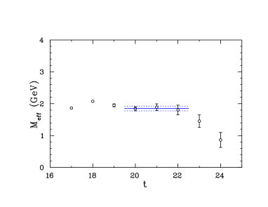
Figure 1: (Color online). Effective mass function for the second $N{1/2}^{-}$ state over 350 configurations from Ref. [7]. The best fit with a mass of 1.85(7) GeV and $\chi^{2}/{\rm{dof}}=0.50$, is also shown.

We refer to the states observed in our correlation matrix analysis as the first, second, third, $\ldots$, odd-parity states, with the first state being the lowest energy state. Remarkably, the correlation function for the first state shows no evidence of a lower-lying scattering threshold state in the Euclidean-time tail. Therefore we turn our attention to the second state of our correlation matrix analysis. We note that this state has relatively strong overlap with our $\chi_{B}$ interpolating field, in contrast to the first state which is dominated by $\chi_{A}$.

Figure 1 presents the effective mass, $M_{\rm eff}(t)=\log(G(t)/G(t+1))$, from Ref. [7] for the second odd-parity state from 350 configurations. The correlation matrix analysis was performed at $t_{0}=18$ relative to the source at $t_{s}=16$ with $\triangle t=2$ such that one seeks a fit commencing at $t_{\rm{min}}=t_{0}=18$. $t_{\rm{max}}=23$ was initialized as the effective mass at $t=24$ was viewed as a transition to noise which commences at $t=25$. The fit satisfying our criteria is illustrated commencing at $t_{\rm{min}}=20$, two time steps after $t_{0}$.

There are two scenarios that could lead to $t_{\rm{min}}>t_{0}$. In the first and most familiar scenario, the number of states participating in the correlation functions of the $8\times 8$ correlation matrix exceed 8 and the higher-energy state contaminations are introducing curvature at early times. In this case further Euclidean time evolution is required to reduce the contributions of the highest states in the spectrum to an insignificant level such that only 8 states are significant in the correlation matrix analysis. Further discussion of this issue is included in the Appendix of Ref. [9].

In practice, one can implement the correlation matrix analysis at later variational times. However, uncertainties grow rapidly. We have noted an insensitivity of the eigenvectors to the variational parameters. This is reflected in the fact that the extracted masses are consistent and insensitive to the variational parameters of $t_{0}$ and $\triangle t$. In conclusion, we accept $t_{\rm{min}}$ in the range $t_{0}\leq t_{\rm{min}}\leq t_{0}+\triangle t$ as providing the best estimate of the eigenstate energy.

In this scenario, where high-energy states are inducing curvature in the correlation function at early times, a lower-lying $N\pi$ scattering state may be present in the projected correlation function. However, its contribution is suppressed relative to the dominant state and its presence results in a negligible systematic error.

In the second scenario, the contribution from a lower lying $N\pi$ scattering state in the projected correlation function is significant. The combination of two states gives rise to curvature in the effective mass at $t=18$ and 19 following the source at $t_{s}=16$. The small $\chi^{2}/{\rm{dof}}=0.50$ of the fit in Fig. 1 provides no hint of a second state and the extracted mass represents a superposition of two states as opposed to a finite-volume QCD eigenstate. In this case the reported mass will contain an undetected systematic error.

The presence and strength of a lower lying $N\pi$ scattering state will be revealed in the large Euclidean time tail of the correlation function. Thus to explore these two scenarios further, we quadruple the number of fermion sources on each configuration and use the full set of 400 configurations available from PACS-CS via the ILDG. In the figures, we refer these results as ‘1600 cfg’ and contrast these results with the earlier ‘350 cfg’ results [7].

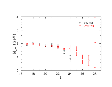
Figure 2: (Color online). Effective mass function $M_{\rm eff}(t)=(1/2)\log(G(t)/G(t+2))$ for the second $N{1/2}^{-}$ state for 1600 configurations is compared with previous results from 350 configurations [7]. A fit from $t=20$ to 27 provides a covariance-matrix based $\chi^{2}/{\rm{dof}}=2.82$ and rejects the hypothesis of a single state at a 99.4% confidence level. The presence of a lower-lying state is manifest in the tail of the effective mass.

Figure 2 illustrates the effective mass obtained from 1600 fermion sources of four different smearing extents at the source and sink; i.e. 25,600 quark propagators. The presence of a second lower-lying contribution to this projected correlation function is now manifest in the drift of the effective mass as a function of Euclidean time. A fit from $t=20$ to 27 provides a covariance-matrix based $\chi^{2}/{\rm{dof}}=2.82$. With seven degrees of freedom the $\chi^{2}$ distribution rejects the hypothesis of a single state at the 99% confidence level and instead indicates the presence of an additional state(s). The new results also confirm that the 350 configuration result at $t=24$ is in fact due to a loss of signal near the onset of noise at $t=25$.

We note that the rejection of the single-state hypothesis contrasts studies of the isovector vector-meson channel of the $\rho$ meson [16] where no evidence of two-particle $\pi\pi$ scattering contributions to the $\rho$-meson correlator was observed when using two-quark operators alone. Only with the specific introduction of four-quark operators, could the $\pi\pi$ contributions to the channel be resolved. This is in accord with the very different nature of the quark flow diagrams and associated couplings describing meson dressings of mesons and baryons in QCD [21, 22].

Having confirmed the presence of at least two states in the projected correlation function, we now consider two-state fits to the projected correlation function.

As explained in Sec. 2, our normalization of the orthogonal eigenvectors $w^{\alpha}$ and subsequent definitions of $u^{\alpha}$ and $v^{\alpha}$ provide $G^{\alpha}(t_{0})=1$ for the projected correlation function. This constraint reduces the standard two-exponential fit function with four parameters

$$G^{\alpha}(t)=\lambda_{1}\,\exp\left(-M_{1}\,(t-t_{s})\right)+\lambda_{2}\,\exp\left(-M_{2}\,(t-t_{s})\right)\,,$$ (32)

to a three parameter function with

$$\lambda_{2}=\frac{1-\lambda_{1}\exp\left(-M_{1}\,(t_{0}-t_{s})\right)}{\exp\left(-M_{2}\,(t_{0}-t_{s})\right)}\,.$$ (33)

This construction ensures $G^{\alpha}(t_{0})=1$ exactly and thus the $\chi^{2}/{\rm dof}$ is evaluated over the interval $t=t_{0}+1$ to $t_{\rm{max}}$. As Fig. 2 indicates a loss of signal in $G^{\alpha}(t)$ at $t=28+2=30$, we commence with the largest interval having $t_{\rm{max}}=29$.

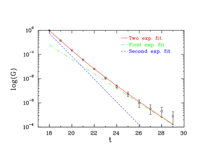
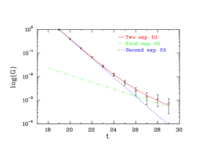
Figure 3: (Color online). (Left) A two exponential fit to the projected correlation function obtained from a generalized eigenvalue analysis at $t_{0}=18$, $t_{0}+\triangle t=20$ relative to the fermion source at $t_{s}=16$. (Right) A similar fit to the projected correlation function obtained from a generalized eigenvalue analysis at $t_{0}=19$, $t_{0}+\triangle t=20$. Dashed and dash-dot lines illustrate the individual exponentials from the fits while the full line presents the sum of exponentials fit to the lattice results.

Figure 3 illustrates two-state fits to the projected correlation function of the second state of the correlation matrix spectrum. The left-hand plot displays the results of a correlation matrix analysis at $t_{0}=18$, $t_{0}+\triangle t=20$ relative to the fermion source at $t_{s}=16$. The right-hand plot illustrates results for a correlation matrix analysis at $t_{0}=19$, $t_{0}+\triangle t=20$. In both cases, the $\chi^{2}/{\rm{dof}}$ is well below one. As is common for two-state fits, the nature of the fits depends sensitively on the earliest time slice considered in the fit.

6.1 $t_{0}=18$ Analysis

Including results at $t=18$ and 19 in the fit, prior to the onset of the plateau in Fig. 2 at $t=20$ results in a fit where both states are given similar weight. The main role of the additional state is to accommodate the curvature in $\log(G)$ at early times. This is consistent with the second scenario described earlier in this section.

Setting $t_{0}$ one step later leads to a very different fit where the additional state is given a very small weight and its main role is to accommodate curvature in the tail of the correlation function. This is consistent with the first scenario described earlier herein.

Table 1 presents variational parameters, fit results, correlated ratios and the $\chi^{2}/{\rm{dof}}$ for these two fits as well as several other closely related fits. The large uncertainties in the results illustrate the interplay between the two exponentials and the importance of establishing correlation matrices that are able to couple strongly to the two-particle components of the QCD eigenstates and enable the isolation of each state.

Table 1: Fitted parameters including masses (in GeV) and coupling strengths ($\lambda$) from two-exponential fits to projected correlation functions obtained with variational parameters $t_{0}$ and $\triangle t$ in an $8\times 8$ correlation matrix analysis. Fits are from $t_{0}$ to $t_{\rm max}$ relative to the source at $t_{s}=16$. The ratio of $M_{1}$ to $M_{2}$ and $\lambda_{1}$ to $\lambda_{2}$ and their correlated errors are also shown. Note, the infinite volume scattering threshold is $M_{N}+m_{\pi}=1.36$ GeV at this second lightest quark mass of the PACS-CS configurations and is expected to be attractive on the finite volume of the lattice.

$t_{0}$	$\triangle t$	$t_{\rm max}$	$M_{1}$	$M_{2}$	$M_{1}/M_{2}$	$\lambda_{1}$	$\lambda_{2}$	$\lambda_{1}/\lambda_{2}$	$\chi^{2}/{\rm{dof}}$
18	1	28	1.54(25)	2.45(41)	0.62(03)	1.83(1.95)	6.22(1.23)	0.29(37)	0.50
18	2	28	1.53(39)	2.36(50)	0.65(05)	1.60(2.83)	6.19(2.02)	0.26(56)	0.48
18	3	28	1.56(43)	2.37(60)	0.65(05)	1.75(3.38)	6.02(2.48)	0.29(71)	0.48
18	1	29	1.49(30)	2.38(40)	0.62(03)	1.48(2.02)	6.43(1.28)	0.23(36)	0.47
18	2	29	1.43(49)	2.26(41)	0.63(11)	1.00(2.53)	6.60(1.77)	0.15(44)	0.36
18	3	29	1.45(56)	2.25(49)	0.64(12)	1.05(3.04)	6.52(2.20)	0.16(56)	0.35
19	1	28	0.91(85)	1.95(11)	0.46(41)	0.12(0.77)	16.25(0.97)	0.01(05)	0.11
19	2	28	1.06(99)	1.97(20)	0.53(48)	0.25(2.54)	16.31(1.58)	0.01(16)	0.16
19	1	29	0.71(68)	1.93(06)	0.37(34)	0.04(0.20)	16.05(0.92)	0.002(12)	0.10
19	2	29	0.78(85)	1.93(08)	0.41(43)	0.06(0.40)	16.09(1.03)	0.004(24)	0.10

While the selection of $t_{0}$ governing where the fit starts plays a significant role, the variation of $\triangle t$ has a negligible effect on the results.

When commencing at $t_{0}=18$, reducing $t_{\rm{max}}$ by one to 28 has little effect on the results. Here the focus is on small times where the uncertainties are small. $M_{1}=1.54(25)$ GeV compares favorably with the infinite volume scattering threshold of $M_{N}+m_{\pi}=1.35$ GeV at this second lightest quark mass of the PACS-CS configurations. However, one is anticipating an attractive interaction on the finite volume lattice and in this light the lattice value is somewhat large.

The best determined value for $M_{2}=2.4(4)$ GeV is larger than the published result [7] of 1.85(7) GeV illustrated in Fig. 1 and presents an explicit case of how an undetected scattering state could contribute to the slope of the lattice correlation function and mask the true mass of the dominant state.

While each of the masses are not accurately determined, the mass ratio is, due to the strong correlation between these two parameters. Similarly the amplitudes of the states are poorly determined but the ratio of the amplitudes $\lambda_{1}/\lambda_{2}$ is the order of $1/10$, large enough to provide an important systematic error as described earlier.

6.2 $t_{0}=19$ Analysis

Turning our attention to $t_{0}=19$, the inclusion of $t_{\rm{max}}=29$ is of some assistance, better constraining both masses. The most accurate result for $M_{2}$ of 1.93(6) GeV compares favorably with the published result from 350 configurations [7] of 1.85(7) GeV. It also agrees well with the same fit of the effective mass from 1,600 configurations producing 1.84(5) GeV, with the $\chi^{2}/{\rm{dof}}=0.3$. This small $\chi^{2}/{\rm{dof}}$ for a single-state fit provides further support that the right-hand panel of Fig. 3 with $t_{0}$ conservatively delayed to $t=19$ is the best representation of the underlying physics.

In this case, the lower-lying state is now addressing the Euclidean time tail of the projected correlator which spoiled the $\chi^{2}/{\rm dof}$ in the fit from $t=20$ to 27 in Fig. 2. The two-state fit $\chi^{2}/{\rm dof}$ of 0.10 to 0.16 argues against dropping any further time slices from the fit. These small values for the $\chi^{2}/{\rm dof}$ are associated with the introduction of not one but two additional parameters to the fit function. One needs both an additional mass and a measure of the relative strengths of the couplings of the two states to the interpolator. The presence of three parameters in the fit function enables an excellent description of the data that would withstand a significant increase in the statistical accuracy of the results.

The lower-lying state is suppressed by one to two orders of magnitude relative to the dominant state in the range $20\leq t\leq 23$ included in the fit of Fig. 1. Here the ratio of amplitudes $\lambda_{1}/\lambda_{2}$ is of order $1/100$ with the low-lying scattering state making a very small contribution revealed only through ample Euclidean time evolution. The range of the low-lying mass, $M_{1}$, readily encompasses the infinite volume scattering threshold of $M_{N}+m_{\pi}=1.35$ GeV and the preference for lower lying values is in accord with the anticipated attractive interaction on the finite volume lattice.

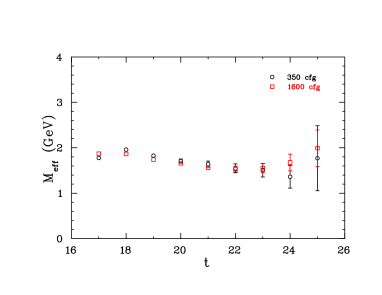
Figure 4: (Color online). Effective mass function $M_{\rm eff}(t)=(1/2)\log(G(t)/G(t+2))$ for the lowest $N{1/2}^{-}$ state for 1600 configurations is compared with previous results from 350 configurations [7]. The projected correlation functions are obtained from an $8\times 8$ correlation matrix analysis at $t_{0}=18$ and $\triangle t=2$. As there is no evidence for a low-lying scattering state contribution in the effective mass tail, the delay of plateau onset is associated with excited state contributions.

Further support for the more cautious $t_{0}=19$ analysis illustrated in the the right hand-panel of Fig. 3 is provided in Fig. 4 presenting the effective mass function for the lowest-lying first odd-parity state observed in our $8\times 8$ correlation matrix analysis. In this case there is no evidence for a low-lying scattering state. A fit from $t=20$ to 24 inclusive provides a $\chi^{2}/{\rm dof}=1.24$ and leaves a 30% chance of finding a higher $\chi^{2}/{\rm dof}$ in a subsequent simulation.

However, significant evolution of the effective mass is observed at early Euclidean time and it is clear that the projected correlation function has small admixtures of additional states. This is due to more than 8 states participating in the correlation functions of the correlation matrix and these may include multi-particle scattering states higher in energy. Indeed Ref. [16] analysing four-quark $\pi\pi$ contributions to the isovector vector correlator of the $\rho$ meson found many $\pi\pi$ scattering contributions before the first excited state observed when using two-quark interpolating fields alone.

Given the direct observation herein of a low-lying multi-particle scattering-state threshold in a “projected” correlation function one must expect similar contributions from the next two-particle zero-momentum scattering-states having the back-to-back momenta allowed on the lattice. Similarly, given the observation of several two-particle scattering-state contributions in the $\rho$ meson channel [16], the curvature observed at early times can be attributed to the higher-energy scattering-state contributions. Thus the analysis with $t_{0}=19$ in the right-hand plot of Fig. 3 is the correct representation of the multi-particle contributions to the nucleon correlator under examination herein. Careful consideration of the $\chi^{2}/{\rm{dof}}$ allows us to circumvent contamination from higher=lying states and ensure we are extracting the finite-volume QCD eigenstate energy.

7 Conclusions

We have revealed the manner in which the absence of a strong coupling to multi-particle components of QCD eigenstates can allow scattering states to be superposed with the dominant state in a projected correlation function from a correlation matrix analysis. Even if the interpolating fields are poor at creating these multi-particle components, QCD dynamics will ensure their formation in the resolution of the eigenstates of QCD,

We have explored two interpretations of how states are superposed to give rise to the observed projected correlation function and illustrated with reference to a real-world example how this superposition of states can impact the results extracted from lattice correlation functions. Given the direct observation herein of a low-lying multi-particle scattering-state threshold in a “projected” correlation function one must expect similar contributions from the next two-particle zero-momentum scattering-states having the back-to-back momenta allowed on the lattice [16]. These states will give rise to curvature in the effective mass at early Euclidean times and therefore the analysis with $t_{0}=19$ relative to the source at $t_{s}=16$ in the right-hand plot of Fig. 3 is the correct representation of the low-lying multi-particle contribution to the nucleon correlator under examination herein.

We have discovered that the low-lying scattering states not observed in Ref. [7] are hidden within the projected correlation functions as very small contributions to the correlation functions suppressed by a factor the order of $1/100$. In the realm where previous fits were performed, their contribution to the correlation function is suppressed by one to two orders of magnitude, as illustrated in the right-hand plot of Fig. 3. As a result, the undetected presence of a lower-lying scattering state has only a small effect on the extracted mass. It is the judicious treatment of the $\chi^{2}/{\rm{dof}}$ that assists in avoiding systematic errors.

The extent to which one can separate multiple states in a single correlator has also been illustrated. It is readily apparent that multi-hadron states must be isolated in the correlation matrix analysis if one is to learn their properties. While effective techniques exist to avoid their effects, discovering their properties is a different matter.

Research is already well underway in exploring the best manner to do this [23, 8, 24, 12]. The aim is to create correlation matrices composed from three- and five-quark operators. Strong coupling to the multi-particle components of the QCD eigenstates, $|\,2\rangle$, is often obtained by projecting the momentum of each of the hadrons participating in the scattering state. Alternative approaches allow the five-quark operators to have strong overlap with both single-particle dominated and multi-particle dominated states and alter this overlap through variation of the fermion propagator source and sink smearing [24]. Through consideration of a variety of approaches on the same underlying set of gauge field configurations one can determine the merits of the various approaches and determine the finite-volume spectrum of QCD in an accurate manner.

References

- [1] J. M. Bulava, et al., Phys. Rev. D79 (2009) 034505. arXiv:0901.0027, doi:10.1103/PhysRevD.79.034505.
- [2] M. S. Mahbub, W. Kamleh, D. B. Leinweber, P. J. Moran, A. G. Williams, Phys. Lett. B707 (2012) 389–393. arXiv:1011.5724.
- [3] J. Bulava, et al., Phys. Rev. D82 (2010) 014507. arXiv:1004.5072, doi:10.1103/PhysRevD.82.014507.
- [4] G. P. Engel, C. B. Lang, M. Limmer, D. Mohler, A. Schafer, Phys. Rev. D82 (2010) 034505. arXiv:1005.1748, doi:10.1103/PhysRevD.82.034505.
- [5] B. J. Menadue, W. Kamleh, D. B. Leinweber, M. S. MahbubarXiv:1109.6716.
- [6] R. G. Edwards, J. J. Dudek, D. G. Richards, S. J. Wallace, Phys. Rev. D84 (2011) 074508. arXiv:1104.5152, doi:10.1103/PhysRevD.84.074508.
- [7] M. S. Mahbub, W. Kamleh, D. B. Leinweber, P. J. Moran, A. G. Williams, Phys.Rev. D87 (2013) 011501. arXiv:1209.0240, doi:10.1103/PhysRevD.87.011501.
- [8] C. Lang, V. Verduci, Phys.Rev. D87 (2013) 054502. arXiv:1212.5055, doi:10.1103/PhysRevD.87.054502.
- [9] M. S. Mahbub, W. Kamleh, D. B. Leinweber, P. J. Moran, A. G. Williams, Phys. Rev. D87, 094506. arXiv:1302.2987, doi:10.1103/PhysRevD.87.094506.
- [10] G. P. Engel, C. Lang, D. Mohler, A. Schaefer, Phys.Rev. D87 (2013) 074504. arXiv:1301.4318.
- [11] C. Alexandrou, T. Korzec, G. Koutsou, T. LeontiouarXiv:1302.4410.
- [12] C. Morningstar, J. Bulava, B. Fahy, J. Foley,Y. Jhang, et al.arXiv:1303.6816.
- [13] C. Michael, Nucl. Phys. B259 (1985) 58.
- [14] M. Luscher, U. Wolff, Nucl. Phys. B339 (1990) 222–252.
- [15] S. Gusken, Nucl. Phys. Proc. Suppl. 17 (1990) 361–364.
- [16] J. J. Dudek, R. G. Edwards, C. E. Thomas, Phys.Rev. D87 (3) (2013) 034505. arXiv:1212.0830, doi:10.1103/PhysRevD.87.034505.
- [17] S. Aoki, et al., Phys. Rev. D 79 (2009) 034503. arXiv:0807.1661.
- [18] M. G. Beckett, et al., Comput. Phys. Commun. 182 (2011) 1208–1214. arXiv:0910.1692, doi:10.1016/j.cpc.2011.01.027.
- [19] Y. IwasakiUTHEP-118.
- [20] B. Efron, Ann. Stat. 29 (1979) 1–26.
- [21] C. Allton, W. Armour, D. B. Leinweber, A. W. Thomas, R. D. Young, Phys.Lett. B628 (2005) 125–130. arXiv:hep-lat/0504022, doi:10.1016/j.physletb.2005.09.020.
- [22] W. Armour, C. Allton, D. Leinweber, A. Thomas, R. Young, Nucl.Phys. A840 (2010) 97–119. arXiv:0810.3432, doi:10.1016/j.nuclphysa.2010.03.012.
- [23] C. Morningstar, et al., Phys. Rev. D83 (2011) 114505. arXiv:1104.3870, doi:10.1103/PhysRevD.83.114505.
- [24] A. L. Kiratidis, W. Kamleh, D. B. Leinweber, PoS LATTICE2012 (2012) 250. arXiv:1301.3591.