Mode coupling in spin torque oscillators

Abstract

A number of recent experimental works have shown that the dynamics of a single spin torque oscillator can exhibit complex behavior that stems from interactions between two or more modes of the oscillator. Examples are observed mode-hopping or mode coexistence. There has been some intial work indicating how the theory for a single-mode (macro-spin) spin torque oscillator should be generalized to include several modes and the interactions between them. In the present work, we derive such a theory starting with the Landau-Lifshitz-Gilbert equation for magnetization dynamics. We compare our result with the single-mode theory, and show how the coupled-mode theory arises as a natural extension of the single-mode theory by including mode interactions.

I Introduction

Since the prediction of spin transfer torque (STT) in 1996Slonczewski (1996); Berger (1996); Ralph and Stiles (2008), whereby a spin-polarized dc current exerts a torque on the local magnetization order parameter, there have been a wealth of theoretical and experimental investigations of phenomena driven by STT. One particular manifestation of STT is the spin torque oscillator (STO). The STO is typically realized in MgO magnetic tunnel junctionsNazarov et al. (2008); Deac et al. (2008); Houssameddine et al. (2009); Zeng et al. (2010); Muduli et al. (2012), or metallic nanocontactsMancoff et al. (2006); Rippard et al. (2004); Silva and Rippard (2008); in both of these, a dc current is driven perpendicularly to two thin stacked magnetic layers, in one of which the magnetization is relatively free to rotate, while in the other the magnetization is held fixed. With the relative magnetization directions and current direction arranged appropriately, STT pumps energy into the STO, and by adjusting the current magntitude, this pumping can be made to cancel the intrinsic dissipative processes in the system. This gives rise to almost undamped oscillations with a very small linewidth. As STOs are potentially useful in technological applications, such as frequency generators or modulators, it is both of practical as well as of fundamental interest to understand the physics of the STO auto-oscillations. Slavin and co-workersSlavin and Tiberkevich (2008); Tiberkevich et al. (2008); Kim et al. (2008); Slavin and Tiberkevich (2009) put forth a comprehensive theory valid for single-mode STOs, that is, STOs for which one mode is relevant and is excited (this is when a macro-spin model is readily applicable). Some striking features of this theory are the effects induced by the inherent nonlinearity of the STOs, for example the behavior of the oscillator linewidth below and above thresholdTiberkevich et al. (2008); Kim et al. (2008); Slavin and Tiberkevich (2009), which is the current at which STT pumping first cancels damping and auto-oscillations are achieved. Recently, there have been several experiments demonstrating the effects of multi-mode STOs, for example mode co-existence and mode-hoppingBerkov and Gorn (2007); Bonetti et al. (2012, 2010); Krivorotov et al. (2008); Lee et al. (2004); Sankey et al. (2005); Muduli et al. (2012); Dumas et al. (2013). Clearly, the interactions between several oscillator modes cannot be described by the single-mode theory but requires a theory that describes the interactions between collective modes, and how the behavior of the collective modes is modified as a consequence of those interactions. A multi-mode theory was first outlined by Muduli, Heinonen, and ÅkermanMuduli et al. (2012, 2012); Heinonen et al. (2013). In particular, these authors argued that the equations describing two-coupled modes could be mapped onto a driven dynamical system, for example used to describe semiconductor ring lasersvan der Sande et al. (2008); Beri et al. (2008). It is known that in the presence of thermal noise, those equations exhibit mode-hopping in certain regions of parameter spaceBeri et al. (2008). A key observation here was that for mode-hopping to be present in a two-mode system, the time derivative of the slowly varying amplitude of one mode must be coupled linearly to the amplitude of the other mode (a so-called ”back-scattering” term). Also, the authors gave some general argument for why mode-hopping is a minimum when the free layer magnetization is anti-parallel to that of the fixed layer, and then increases as the orientation moves away from anti-parallelMuduli et al. (2012). The purpose of the present work is to derive the equations for coupled modes from first principles (the micromagnetic Landau-Lifshitz-Gilbert equation), and to analyze the ensuing behavior of the system. We will also to compare our results with the single-mode theory and to discuss in some detail how the present work is a generalization of the single-mode theoryTiberkevich et al. (2008); Kim et al. (2008); Slavin and Tiberkevich (2009). We will show how the linear backscattering term arises naturally in a system with a small number, e.g., two, of dominant modes but in which there is a bath of many modes. This bath provides effective interactions between the dominant modes when the bath is integrated out and the equations projected onto the subspace of dominant modes. We will also show that there are additional terms that arise when the free layer and fixed layer magnetizations are at some angle $\beta$ away from parallel or anti-parallel. These terms open up new scattering channels between modes, and therefore lead to more mode-mode interactions, and provide a mechanism for the observedMuduli et al. (2012) increased mode-hopping away from parallel or anti-parallel free and fixed layer magnetizations. The geometry we use is specifically adapted for a magnetic tunnel junction with in-plane magnetization and an in-plane external field, although we will also discuss some other geometries.

II Micromagnetic equations

Our starting point is a soft ferromagnetic system, for example a thin film. We describe the local magnetization by a director $\hat{m}_{i}$ for discrete sites $i=1,2,\ldots N$, with $|\hat{m}_{i}|=1$. The LLG equation including damping and spin torque is then

$$\frac{d\hat{m}_{i}}{dt}=-\gamma\hat{m}_{i}\times{\mathbf{H}}_{{\rm eff},i}-\frac{\gamma\alpha}{1+\alpha^{2}}\hat{m}_{i}\times\left[\hat{m}_{i}\times{\mathbf{H}}_{{\rm eff},i}\right]+\gamma a_{J}\hat{m}_{i}\times\left[\hat{m}_{i}\times\hat{M}\right].$$ (1)

Here, $\gamma$ is the gyromagnetic ratio, $\alpha\ll 1$ the dimensionless damping, $a_{J}$ the effective field due to STT, and $\hat{M}$ the (uniform) magnetization direction of the fixed layer; the effective field ${\mathbf{H}}_{{\rm eff},i}$ includes exchange, demagnetizing fields, and an external applied field ${\mathbf{H}}_{\rm ext}=H_{\rm ext}\hat{x}$. We will not here include Oersted fields generated by the currents in the system as they are not important for the present analysis, although it has shown that these fields play an important role in the interactions between certain modes in nano-contact STOsDumas et al. (2013). We are also ignoring the so-called field-like, or perpendicular, spin torqueZhang et al. (2002) as this can be absorbed into the definition of the external field. We shall combine exchange and demagnetizing fields into a single field ${\mathbf{H}}_{{d},i}$ and note that in general we can write

$$H_{d,i,\delta}=\sum_{i^{\prime},\epsilon}D_{i,i^{\prime};\delta,\epsilon}m_{i^{\prime},\epsilon},\,\,\delta,\epsilon=x,y,z,$$ (2)

where $D_{i,i^{\prime};\delta,\epsilon}$ is a generalized demagnetizing tensor that includes near-neighbor exchange. We shall also assume that the anisotropy is negligible, and that the equilibrium free layer magnetization direction is aligned with the external field along the $\hat{x}$ axis. This applies, for example, to magnetic tunnel junctions with an in-plane external field, or to systems with a large ($H_{\rm ext}\gg 4\pi M_{S}$) external field perpendicular to the planes of the magnetic layers. Figure 1 depicts the equilibrium magnetization in the free layer of a circular magnetic tunnel junction STO of diameter $d=240$ nm obtained from micromagnetic simulations with parameters appropriate for the systems in Ref. Muduli et al., 2011. In the figure, the pinned layer and reference layer magnetizations are approximately (these layers are also treated micromagnetically) at $45^{\circ}$ and $-135^{\circ}$ degrees to the $x$-axis, and there is an external field of magnitude 450 Oe applied in the $xy$-plane at $85^{\circ}$ to the $x$-axis (in an actual magnetic tunnel juction, there are three magnetic layers, and the reference layer is the one next to the free layer and is responsible for the spin transfer torque).

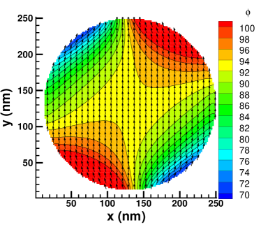
Figure 1: (Color online) Micromagnetic equilibrium magnetization in the free layer of a circular magnetic tunnel junction of diameter 240 nm. The pinned and reference layer magnetizations (not shown) are at $45^{\circ}$ and $-135^{\circ}$ degrees to the $x$-axis, and there is and external field of 450 Oe applied at $85^{\circ}$ to the $x$-axis. The color scale shows the angle $\phi$ between the local magnetization and the $x$-axis.

The figure shows that while the magnetization is not perfectly aligned with the external field everywhere, the maximum deviation is small, about $15^{\circ}$, and an expansion in deviations from alignment with the uniform external field is reasonable and should converge rapidly. It is of course easy to generalize to an arbitrary local effective field direction and with a non-uniform equilibrium magnetization in the direction of the local net magnetic field, but that does introduce more variables. We prefer to keep the discussion relatively simple and transparent, and also with the specific application in mind of a magnetic tunnel junction STO with an in-plane external field, or a nanocontact STO with a strong out-of-plane external field. For simplicity, we will use units in which $\gamma=1$, and because $\alpha\ll 1$ we will ignore terms of order $\alpha^{2}$. In terms of components, the LLG equation is then

$$\frac{dm_{x,i}}{dt} = -\left(m_{i,y}H_{d,i,z}-m_{i,z}H_{d,i,y}\right)+\alpha\left(1-m_{i,x}^{2}\right)\left(H_{\rm ext}+H_{d,i,x}\right)-\alpha m_{i,x}\left(m_{i,y}H_{d,i,y}+m_{i,z}H_{d,i,z}\right)$$ (3)

$$-a_{J}\left(1-m_{i,x}^{2}\right)\cos\beta-a_{J}m_{i,x}m_{i,y}\sin\beta$$

$$\frac{dm_{y,i}}{dt} = -\left[m_{i,z}\left(H_{d,i,x}+H_{\rm ext}\right)-m_{i,x}H_{d,i,z}\right]+\alpha\left(1-m_{i,y}^{2}\right)H_{d,i,y}-\alpha m_{i,y}\left[m_{i,x}\left(H_{d,i,x}+H_{\rm ext}\right)+m_{i,z}H_{d,i,z}\right]$$ (4)

$$+a_{J}\left(1-m_{i,y}^{2}\right)\sin\beta-a_{J}m_{i,x}m_{i,y}\sin\beta$$

$$\frac{dm_{z,i}}{dt} = -\left[m_{i,x}H_{d,i,y}-m_{i,y}\left(H_{\rm ext}+H_{d,i,x}\right)\right]+\alpha\left(1-m_{i,z}^{2}\right)H_{d,i,z}-\alpha m_{i,z}\left[m_{i,x}\left(H_{d,i,x}+H_{\rm ext}\right)+m_{i,y}H_{d,i,y}\right]$$ (5)

$$+a_{J}m_{i,z}\left(m_{i,x}\cos\beta-m_{i,y}\sin\beta\right).$$

Next, we introduce the generalized local non-linear Holstein-Primakoff transformation of Slavin and co-workersSlavin and Tiberkevich (2008, 2009) that transforms the two degrees of freedom of each director $\hat{m}_{i}$ to a complex variable $c_{i}$,

$$c_{i}=\frac{m_{y,i}-im_{z,i}}{\sqrt{2\left(1+m_{x,i}\right)}},$$ (6)

with the inverse transformation

$$\hat{m}_{i}=\sqrt{1-|c_{i}|^{2}}\left[\left(c_{i}+c^{*}_{i}\right)\hat{y}+i\left(c_{i}-c_{i}^{*}\right)\hat{z}\right]+\left(1-2|c_{i}|^{2}\right)\hat{x}.$$ (7)

In terms of the local variables $c_{i}$, we can write the fields ${\mathbf{H}}_{d,i}$ as

$$H_{d,i,x} = \sum_{i^{\prime}}\left[D_{i,i^{\prime};x,x}\left(1-2|c_{i^{\prime}}|^{2}\right)+D_{i,i^{\prime};x,y}\sqrt{1-|c_{i^{\prime}}|^{2}}\left(c_{i^{\prime}}+c_{i^{\prime}}^{*}\right)+D_{i,i^{\prime};x,z}i\sqrt{1-|c_{i^{\prime}}|^{2}}\left(c_{i^{\prime}}-c_{i^{\prime}}^{*}\right)\right]$$ (8)

$$H_{d,i,y} = \sum_{i^{\prime}}\left[D_{i,i^{\prime};y,x}\left(1-2|c_{i^{\prime}}|^{2}\right)+D_{i,i^{\prime};y,y}\sqrt{1-|c_{i^{\prime}}|^{2}}\left(c_{i^{\prime}}+c_{i^{\prime}}^{*}\right)+D_{i,i^{\prime};y,z}i\sqrt{1-|c_{i^{\prime}}|^{2}}\left(c_{i^{\prime}}-c_{i^{\prime}}^{*}\right)\right]$$ (9)

$$H_{d,i,z} = \sum_{i^{\prime}}\left[D_{i,i^{\prime};z,x}\left(1-2|c_{i^{\prime}}|^{2}\right)+D_{i,i^{\prime};z,y}\sqrt{1-|c_{i^{\prime}}|^{2}}\left(c_{i^{\prime}}+c_{i^{\prime}}^{*}\right)+D_{i,i^{\prime};z,z}i\sqrt{1-|c_{i^{\prime}}|^{2}}\left(c_{i^{\prime}}-c_{i^{\prime}}^{*}\right)\right]$$ (10)

By multiplying Eq. (5) by $i$ and subtracting the result from Eq. (4), and also using $m_{x,i}=1-2|c_{i}|^{2}$ from Eq. (7) in Eq. (3), we obtain the following equations:

$$\frac{d}{dt}\left[2\sqrt{1-|c_{i}|^{2}}c_{i}\right] = \left(1-2|c_{i}|^{2}\right)\left(H_{d,i,z}+iH_{d,i,y}\right)-2i\sqrt{1-|c_{i}|^{2}}c_{i}\left(H_{\rm ext}+H_{d,i,x}\right)$$ (11)

$$-2\alpha\sqrt{1-|c_{i}|^{2}}c_{i}\left[m_{i,x}\left(H_{\rm ext}+H_{d,i,x}\right)+m_{i,y}H_{d,i,y}+m_{i,z}H_{d,i,z}\right]$$

$$+\alpha\left(H_{d,i,y}-iH_{d,i,z}\right)+2a_{J}\sqrt{1-|c_{i}|^{2}}c_{i}\left(m_{i,x}\cos\beta-m_{i,y}\sin\beta\right)+a_{J}\cos\beta$$

$$-2\frac{d}{dt}|c_{i}|^{2} = -\sqrt{1-|c_{i}|^{2}}\left[\left(c_{i}+c_{i}^{*}\right)H_{d,i,z}-i\left(c_{i}-c_{i}^{*}\right)H_{d,i,y}\right]+4\alpha\left(1-|c_{i}|^{2}\right)|c_{i}|^{2}\left(H_{\rm ext}+H_{d,i,x}\right)$$ (12)

$$-\alpha\left(1-2|c_{i}|^{2}\right)\sqrt{1-|c_{i}|^{2}}\left[\left(c_{i}+c_{i}^{*}\right)H_{d,i,y}+i\left(c_{i}-c_{i}^{*}\right)H_{d,i,z}\right]$$

$$-4a_{J}\cos\beta\left(1-|c_{i}|^{2}\right)|c_{i}|^{2}-a_{J}\left(1-2|c_{i}|^{2}\right)\sqrt{1-|c_{i}|^{2}}\left(c_{i}+c_{i}^{*}\right)\sin\beta.$$

Finally, we combine Eqs. (11 - 12) and use

$$\frac{d}{dt}\left[2\sqrt{1-|c_{i}|^{2}}c_{i}\right]=2\sqrt{1-|c_{i}|^{2}}\frac{dc_{i}}{dt}-\frac{c_{i}}{\sqrt{1-|c_{i}|^{2}}}\frac{d|c_{i}|^{2}}{dt}$$ (13)

to obtain

$$\frac{dc_{i}}{dt} = -\frac{(iH_{d,i,y}+H_{d,i,z})(-2+3|c_{i}|^{2})}{4\sqrt{1-|c_{i}|^{2}}}-i(H_{\rm ext}+H_{d,i,x})c_{i}-\frac{(iH_{d,i,y}-H_{d,i,z})c_{i}^{2}}{4\sqrt{1-|c_{i}|^{2}}}$$ (14)

$$+\alpha\frac{(H_{d,i,y}-iH_{d,i,z})\left[{2+|c_{i}|^{2}(-3+2|c_{i}|^{2})}\right]}{4\sqrt{1-|c_{i}|^{2}}}-\alpha c_{i}(H_{\rm ext}+H_{d,i,x})(1-|c_{i}|^{2})+\alpha c_{i}^{2}\frac{(H_{d,i,y}+iH_{d,i,z})(-3+2|c_{i}|^{2})}{4\sqrt{1-|c_{i}|^{2}}}$$

$$+a_{J}\frac{\left[{2+|c_{i}|^{2}(-3+2|c_{i}|^{2})}\right]\sin[\beta]}{4\sqrt{1-|c_{i}|^{2}}}+a_{J}c_{i}(1-|c_{i}|^{2})\cos[\beta]+a_{J}c_{i}^{2}\frac{(-3+2|c_{i}|^{2})\sin[\beta]}{4\sqrt{1-|c_{i}|^{2}}}$$

The somewhat unpleasant-looking Eq. (14), together with Eqs. (8 - 10), is equivalent to the traditional LLG equation and describes the full non-linear magnetization motion in the presence of damping and (in-plane) STT. The advantage of this form compared to the LLG form is that it allows for a systematic expansion in powers of $c_{i}$ to derive the effective time-evolution of coupled modes. For STT auto-oscillators, we must also include a non-linear dependence of the damping $\alpha$ on the oscillator powerSlavin and Tiberkevich (2008) – otherwise we will not get stable oscillations above threshold – and we will in general write $\alpha=\alpha_{G}(1+q_{1}\xi^{2})$, where $\xi$ is a dimensionless measure of the oscillator energy.

III Non-conservative torques

We will first use Eq. (14) to analyze the effect of the non-conservative torques on an auto-oscillator. By assumption, the magnetization motion is oscillatory with a period $\tau$, and the magnetization amplitude remains constant or invariant under long times. The dissipation of the system is described by the time-rate of change of the oscillator power, proportional to $\sum_{i}|c_{i}|^{2}$. For simplicity, and ease of notation, we now use a macro-spin modelLi and Zhang (2003) with a single amplitude $c$. The rate of dissipation is then given by

$$\frac{d}{dt}|c|^{2} = \sqrt{1-|c|^{2}}\left[\Re(c)H_{d,z}+\Im(c)H_{d,y}\right]$$ (15)

$$+\frac{1}{\sqrt{1-|c|^{2}}}\left\{\left[\Re(c)\left(a_{J}\sin\beta+\alpha H_{d,y}\right)-\alpha H_{d,z}\Im(c)\right]\left[1+|c|^{2}\left(-3+2|c|^{2}\right)\right]\right\}$$

$$-2\left(1-|c|^{2}\right)|c|^{2}\left[\alpha\left(H_{\rm ext}+H_{d,x}\right)-a_{J}\cos\beta\right].$$

Here $\Re(c)$ and $\Im(c)$ are the real and imaginary parts of $c$, respectively. For simplicity, we also assume that the demagnetizing tensor is diagonal (this is not a very drastic assumption for elliptical systems) so that $H_{d,y}=-Ym_{y}=-2Y\sqrt{1-|c|^{2}}\Re(c)$ and $H_{d,z}=-Zm_{z}=2Z\sqrt{1-|c|^{2}}\Im(c)$, with $Y$ and $Z$ real numbers. Then $\frac{1}{\sqrt{1-|c|^{2}}}\Re(c)H_{d,y}=-2Y\left[\Re(c)\right]^{2}$ and $\frac{1}{\sqrt{1-|c|^{2}}}\Im(c)H_{d,z}=2Z\left[\Im(c)\right]^{2}$. We demand that averaged over a period $\tau$, the dissipation is zero, so that

$$\langle\frac{d}{dt}|c|^{2}\rangle=\frac{1}{\tau}\int_{t}^{t+\tau}\frac{d}{dt}|c(t^{\prime})|^{2}\,dt^{\prime}=0.$$ (16)

For an oscillatory motion we can assume

$$\frac{1}{\tau}\int_{t}^{t+\tau}\left[\Re(c(t^{\prime}))\right]^{2}\,dt^{\prime}=\overline{c}^{2}>0,$$ (17)

which defines the number $\overline{c}$. The motion will in general be eccentric with eccentricity $\epsilon$, so

$$\frac{1}{\tau}\int_{t}^{t+\tau}\left[\Im(c(t^{\prime}))\right]^{2}\,dt^{\prime}\approx\epsilon\overline{c}^{2}.$$ (18)

Futhermore, for oscillatory motion we have

$$\frac{1}{\tau}\int_{t}^{t+\tau}\Re[c(t^{\prime})]\,dt^{\prime}\approx 0\approx\frac{1}{\tau}\int_{t}^{t+\tau}\Re[c(t^{\prime})]\Im[c(t^{\prime})]\,dt^{\prime}.$$ (19)

To ${\cal O}(c^{2})$ we then obtain

$$\langle\frac{d}{dt}|c|^{2}\rangle=-(Y+\epsilon Z)\alpha_{G}-\left[\alpha_{G}\left(H_{\rm ext}+\overline{H}_{d,x}\right)-a_{J}\cos\beta\right]\left[1+\epsilon\right]=0,$$ (20)

where $\overline{H}_{d,x}$ is the equilibrium demagnetizing field in the $x$ direction, and a factor of $\overline{c}^{2}$ cancels out. This analysis allows us to draw three conclusions: (i) the time-dependent demagnetizing fields enhance the average dissipation by a factor of $(Y+\epsilon Z)\alpha$; (ii) only the average dissipation is zero, but not the instantaneous dissipation, and during some fraction of a period net energy is pumped into the system, and during some other fraction of a period net energy is dissipatedMuduli et al. (2012); (iii) as $\beta\to\pi/2$ the pumping through STT becomes less and less effective to offset dissipative losses and it becomes in general impossible to obtain self-sustained auto-oscillations. The threshold current is the current at which the average dissipation is zero. From Eq. (20) we see that the spin torque effective field $a_{J}$, which is proportional to the current, and $\cos\beta$ enters as a product. This implies that the threshold current increases as $1/\cos\beta$ as the equilibrium magnetization direction is rotated away from the direction of the reference layer. An increase in threshold current with angle $\beta$ has indeed been observed experimentallyMuduli et al. (2012). The dependence on the product $a_{j}\cos\beta$ also implies an invariance: if a decrease in $\cos\beta$ is offset by an increase in $a_{J}$ by increasing the current such that the product $a_{J}\cos\beta$ is constant the system is invariant. This is not consistent with experimental observations, where, for example, mode-hopping increases dramatically as $\cos\beta$ is decreasedMuduli et al. (2012). As we will argue below, this can only be caused by by the apperance of terms in $a_{J}\sin\beta$ in the coupled-mode equations.

IV Comparison with singe-mode theory

It is instructive to compare Eq. (14) with the single-mode theory. To this end, we assume that there is a single macro-spin, and also assume that the demagnetizing tensor is diagonal, $D_{xx}=-X$, $D_{yy}=-Y$, and $D_{zz}=-Z$. Inserting this, and the transformations Eq. (7) and expanding to third order, we obtain after a little algebra

$$\frac{dc}{dt} = -\frac{i}{2}Y(c+c^{*})\left(1-\frac{3}{2}|c|^{2}-\frac{1}{2}c^{2}\right)-\frac{i}{2}Z(c-c^{*})\left(1-\frac{3}{2}|c|^{2}+\frac{1}{2}c^{2}\right)-icH_{\rm ext}+icX(1-2|c|^{2})$$ (21)

$$-\frac{\alpha}{2}Y(c+c^{*})\left(1-\frac{3}{2}|c|^{2}-\frac{3}{2}c^{2}\right)-\frac{\alpha}{2}Z(c-c^{*})\left(1-\frac{3}{2}|c|^{2}+\frac{3}{2}c^{2}\right)-\alpha cH_{\rm ext}(1-|c|^{2})+\alpha cX(1-3|c|^{2})$$

$$+\frac{a_{J}}{2}\sin\beta\left(1-|c|^{2}-\frac{3}{2}c^{2}\right)+a_{J}c(1-|c|^{2})\cos\beta.$$

The linearized conservative part of this equation is

$$\frac{dc}{dt} = -\frac{i}{2}Y(c+c^{*})-\frac{i}{2}Z(c-c^{*})-iH_{\rm ext}c+iXc$$ (22)

$$= -i\left\{\left[\frac{1}{2}\left(Y+Z\right)+\left(H_{\rm ext}-X\right)\right]c+\frac{1}{2}\left(Y-Z\right)c^{*}\right\},$$

with eigenvalue $\omega^{2}=\left[\left(H_{\rm ext}-X\right)+Y\right]\left[\left(H_{\rm ext}-X\right)+Z\right]$. We can diagonalize Eq. (22) by introducing a complex variable $a$ such that $c=ua-v{a}^{*}$ with

$$u = \sqrt{\frac{\left[H_{\rm ext}-X+\frac{1}{2}\left(Y+Z\right)\right]+\omega}{2(H_{\rm ext}-X)+(Y+Z)}}=\sqrt{\frac{b+\omega}{2b}}$$ (23)

$$v = \sqrt{\frac{\left[H_{\rm ext}-X+\frac{1}{2}\left(Y+Z\right)\right]-\omega}{2(H_{\rm ext}-X)+(Y+Z)}}=\sqrt{\frac{b-\omega}{2b}},$$ (24)

where $b=(H_{\rm ext}-X)+\frac{1}{2}(Y+Z)$. We also define $n=\frac{1}{2}(Y-Z)$ so that $\omega^{2}=b^{2}-n^{2}$. Inverting the relation between $a$ and $c$ we get

$$a=\frac{uc+vc^{*}}{u^{2}-v^{2}}$$ (25)

and $u^{2}-v^{2}=\frac{1}{\omega}\left[H_{\rm ext}-X+\frac{1}{2}(Y+Z)\right]=b/\omega$ and $u^{2}+v^{2}=1$. With this in mind, we can re-write Eq. (21) as

$$\frac{dc}{dt} = -i\left[bc+nc^{*}\right]\left[1-\frac{3}{2}|c|^{2}\right]\left[1-i\alpha\right]$$ (26)

$$-\frac{i}{2}\left(3H_{\rm ext}+X\right)c|c|^{2}+\frac{i}{2}nc^{3}+\frac{i}{4}\left(Y+Z\right)c|c|^{2}$$

$$-\frac{\alpha}{2}\left(H_{\rm ext}+3X\right)c|c|^{2}+\frac{3\alpha}{2}nc^{3}+\frac{3\alpha}{4}\left(Y+Z\right)c|c|^{2}$$

$$+\frac{a_{J}}{2}\sin\beta\left(1-|c|^{2}-\frac{3}{2}c^{2}\right)+a_{J}\cos\beta c(1-|c|^{2}).$$

The conservative parts of the equation of motion for $c$ can be derived from a hermitian Hamiltonian $H$ by $dc/(dt)=-i\partial H/(\partial c^{*})$, where

$$H=b|c|^{2}+\frac{n}{2}\left(c^{*2}+c^{2}\right)-\frac{n}{2}\left(c^{3}c^{*}+cc^{*3}\right)+\frac{1}{4}\left[3H_{\rm ext}+X-\frac{1}{2}(Y+Z)\right]|c|^{4}.$$ (27)

We note that this is different in structure from the Hamiltonian of Slavin and Tiberkevich (Eq. (3.16) in Ref. Slavin and Tiberkevich, 2008) in that Eq. (27) contains no cubic terms. This just stems from our choice of geometry in which the magnetization is aligned with the external field; if the external field has components transverse to the equilibrium magnetization, quadratic terms will appear in the equation of motion Eq. (14) with ensuing cubic terms in the Hamiltonian.

Finally, we introduce a variable $m=\frac{1}{2}(Y+Z)$, expand $\alpha=\alpha_{G}(1+q_{1}|a|^{2})$ and write Eq. (26) in terms of $a$ (see Appendix A for details):

$$\frac{da}{dt} = -i\omega a-\omega a\alpha_{G}\left[1+q_{1}|a|^{2}\right]+\frac{3i\omega}{2}a\left[|a|^{2}-\frac{n}{2b}\left(a^{2}+a^{*2}\right)\right][1-i\alpha]$$ (28)

$$-\frac{i}{2}\left[3H_{\rm ext}+X-m\right]\left[\frac{2b^{2}+n^{2}}{2b\omega}a|a|^{2}-\frac{3n}{2\omega}a^{*}|a|^{2}-\frac{n}{2\omega}a^{3}+\frac{n^{2}}{2b\omega}{a}^{*3}\right]$$

$$+\frac{in}{2}\left[\frac{3n^{2}}{2b\omega}a^{*}|a|^{2}-\frac{3n}{2\omega}a|a|^{2}+\frac{b^{2}+\omega^{2}}{2b\omega}a^{3}-\frac{n}{2\omega}{a}^{*3}\right]$$

$$-\frac{\alpha}{2}\left[H_{\rm ext}+3X-3m\right]\left[a|a|^{2}-\frac{n}{2b}\left(a^{3}+a^{*}|a|^{2}\right)\right]$$

$$+\frac{3\alpha n}{2}\left[a^{3}+\frac{n}{2b}{a}^{*3}-\frac{3n}{2b}a|a|^{2}\right]$$

$$+\frac{a_{J}}{2}\frac{b}{\omega}\sin\beta\sqrt{\frac{b+n}{b}}\left[1+\frac{3n-2b}{2b}|a|^{2}+\frac{5n-6b}{4b}a^{2}-\frac{n}{4b}{a}^{*2}\right]$$

$$+a_{J}\cos\beta a\left[1-|a|^{2}+\frac{n}{2b}\left(a^{2}-a^{*2}\right)\right].$$

Equation (28) looks rather complicated in that it contains all cubic terms in $a$ and $a^{*}$, and not just cubic terms of the form $a|a|^{2}$. However, for the special case $n=0$ (in which case $\omega=b$), the magnetization motion is circularly polarized ($c=a$) and the equation of motion for $a$ attains a very simple form,

$$\frac{da}{dt} = -i\omega a-\omega a\alpha_{G}\left[1+q_{1}|a|^{2}\right]+\frac{3i\omega}{2}a|a|^{2}[1-i\alpha]-\frac{i}{2}\left[3H_{\rm ext}+X-m\right]a|a|^{2}$$ (29)

$$-\frac{\alpha}{2}\left[H_{\rm ext}+3X-3m\right]a|a|^{2}+\frac{a_{J}}{4}\sin\beta\left[2|a|^{2}-3a^{2}\right]+a_{J}\cos\beta a\left[1-|a|^{2}\right].$$

It is clear that the general equation Eq. (28) has an expansion in $|a|^{2}$ only if $n=0$, which means $Y=Z$ or $Y=Z=0$, and if $\sin\beta=0$. This is the case, for example, for the magnetization in a continuous thin film and the external field ($H_{\rm ext}>4\pi M_{S}$) applied perpendicularly to the film plane, in which case $X=4\pi M_{S}$, and with the fixed layer magnetization perpendicular to the plane, so that $\sin\beta=0$, or for an in-plane circular magnetic tunnel junction with the external field aligned with the fixed layer magnetization direction. But for a general object, such as a non-circular patterned magnetic tunnel junction or a nanocontact, $Y\not=Z$, and an expansion in $a$ will contain all terms in $a$ and $a^{*}$. The origin of these latter terms in the conservative torque comes from the time-derivative of $|c|^{2}$, Eq. (12). The conservative third-order terms can be derived from a quartic Hamiltonian. For a single-mode (macrospin) STO only the fourth-order term in $|a|^{4}$ in the Hamiltonian is relevant as other fourth-order terms do not lead to energy-conserving processes, and this term generates the term in $a|a|^{2}$ in the equation of motion responsible for the non-linear frequency shift, which then depends only on the oscillator power (or energy). For multi-mode systems, however, the cubic and higher-order terms both in the conservative and non-conservative parts of the equation of motion have to be considered, and they lead to energy flow between different modes of the system (e.g., mode-hopping) as well as modified damping.

V Mode equations

We will now proceed to derive effective equations for the slow time-behavior of modes in the presence of coupling. By slow we here mean time-scales much larger than characteristic resonance periods of the system, which are of the order of 0.1 - 1 ns; we will make this more precise below. The strategy we will use is very similar to that used in physical optics, where Ansatz solutions are typically made for solutions that are linear combinations of eigenmodes, and the coefficients are slowly time dependentSorel et al. (2002, 2003). To be specific, we will consider a system where two modes, labeled 1 and 2, are dominant. This can be a system such as the one in Ref. Muduli et al., 2011 where the uniform FMR mode is most strongly excited by the spin transfer torque, but where there is mode hopping between this mode and another mode, indicative of strong couplings between those modes, or it can be a system that is close to a mode crossing, such as the system in Ref. Muduli et al., 2012. We shall also assume that $\omega_{1}$ and $\omega_{2}$ are the two lowest frequencies in the system, and that there is a finite gap between $\omega_{i}$ and $\omega_{n}$, where $i=1,2$ and $n=3,4,\ldots$. Figure 2 depicts an experimental example of such a spectrum.

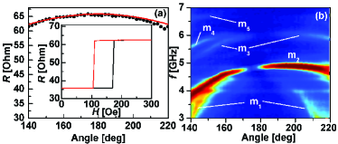
Figure 2: (Color online)(a) Experiment (circles) and calculated (solid line) resistance versus in-plane field angle $\varphi$ at $H$=450 Oe, where $\varphi=180^{\circ}$ corresponds to anti-parallel alignment of the free layer and the reference layer. The inset shows magnetoresistance loop measured at $\varphi=180^{\circ}$. (b) Map of power (dB) vs frequency and in-plane field angle for $I$=8 mA and $H$=450 Oe showing the free layer modes. From Ref. Muduli et al., 2012 (reproduced with permission).

In order to express a solutions in modes, we must specify a reference system for which the modes are well defined. We will use the linearized conservative system as a reference. This system is described by

$$\frac{dc_{i}}{dt}=-\frac{1}{2}(iH_{d,i,y}+H_{d,i,z})-i(H_{\rm ext}+H_{d,i,x})c_{i}.$$ (30)

This is a linear conservative system that admits a family of $N$ orthonormal (complex) eigenvectors $\left\{d_{n}\right\}$, $n=1,2\ldots,N$, that span the range of the linearized equation, with real eigenvalues $\omega_{n}$:

$$\frac{d}{dt}d_{i,n}(t)=\frac{d}{dt}d_{i,n}{\rm e}^{-i\omega_{n}t}=-i\omega_{n}d_{i,n}{\rm e}^{-i\omega_{n}t}=-\frac{1}{2}(iH_{d,i,y}+H_{d,i,z})-i(H_{\rm ext}+H_{d,i,x})d_{i,n},\,i=1,2\ldots,N.$$ (31)

We will use short-hand notation $|d_{n}\rangle$ and $\langle d_{n}|$ for the vector $(d_{1,n},d_{2,n},\ldots,d_{N,n})$ and its adjoint, respectively; the orthogonality and completeness can then be written

$$\langle d_{n}|d_{n^{\prime}}\rangle=\sum_{i}d_{i,n}^{*}d_{i,n^{\prime}}=\delta_{n,n^{\prime}},$$ (32)

and

$$\frac{1}{2\pi}\int_{-\infty}^{\infty}{\rm e}^{-i(\omega_{n}-\omega_{n^{\prime}})t}\,dt=\delta_{n,n^{\prime}}.$$ (33)

We then expand the magnetization motion in the basis $\left\{{d_{n}}\right\}$

$$|c(t)\rangle=\sum_{n}A_{n}(t)|d_{n}\rangle{\rm e}^{-i\omega_{n}t},$$ (34)

where we assume that the complex coefficients $A_{n}(t)$ have a slow time dependence, that is, the time-scale of variation of $A_{n}(t)$ is much larger than $(\omega_{m})^{-1}$ for all $n,m=1,2,\ldots,N$. We insert the expansion Eq. (34) in the equation for the time evolution of the magnetization, Eq.  (14) and project with $\langle d_{n^{\prime}}|$. The left-hand side of the resulting equation then becomes simply $dA_{n^{\prime}}(t)/(dt){\rm e}^{-i\omega_{n^{\prime}}t}-i\omega_{n^{\prime}}A_{n^{\prime}}(t){\rm e}^{-i\omega_{n^{\prime}}t}$. The second term proportional to $\omega_{n^{\prime}}$ is canceled by construction by the linear conservative part on the right-hand side of the equation. The remainder of the right-hand side is a bit of a mess, and contains projections of the non-linear conservative parts as well as the non-conservative parts on $\langle d_{n^{\prime}}|$; note that these terms will in general mix different modes $|d_{n}\rangle$ and $|d_{m}\rangle$. Rather than writing out explicitly here what the terms look like, we will instead systematically analyze the terms of different order in $c_{i}$. The general procedure we will follow is to expand all $c_{i}$’s in the basis $|d_{n}\rangle$, and then multiply both sides of the equation with ${\rm e}^{i\omega_{n^{\prime}}t}$ and integrate over time. The crucial assumption now is that the time dependence of $A_{n}(t)$ is sufficiently slow that it can be held constant during the time integration and moved outside of the integral, while for the integration over exponential factor, we can use Eq. (33). This means we can also ignore correlations between $A_{n}(t)$ and $A_{n^{\prime}}(t)$ on times of the order of $\omega_{m}^{-1}$ for all $n,n^{\prime},m$ while the projected solutions onto modes 1 and 2 will couple $A_{1}(t)$ and $A_{2}(t)$ with temporal correlations on time scales much larger than $\omega_{m}^{-1}$ for all $m$. Each time-integration will then give rise to a condition on the frequency components. These kinds of terms with the condition on the frequencies are entirely analogous to a magnon-magnon scattering vertex, with the condition on the frequencies corresponding to energy conservation at the vertex. In spin wave Hamiltonian theory, the Holstein-Primakoff transformation is usually applied, and a subsequent expansion of $\sqrt{1-\hat{n}_{i}}$, where $\hat{n}_{i}$ is the(bosonic) spin number operator at site $i$, leads to magnon interactions in which magnons scatter off each other. Spin torque oscillators typically have large enough amplitudes that nonlinear processes are important and have to be included. Therefore, the expansions in $|c_{i}|$ and subsequent expansions of $c_{i}$ in eigenmode amplitudes $|A_{n}|$ have to go beyond linear terms, and processes that involve more than two quanta of spin waves have to be considered. This is how linear terms like $dA_{1}/dt\propto A_{2}(t)$ can arise as nonlinear processes that include a bath of magnons give some flexibility in satisfying energy conservation in the scattering processes. We shall here expand only up to third order although we will discuss fourth-order contributions that enter because of the terms in $a_{J}\sin\beta$, as well some higher-order contributions. For ease of notation, we shall also assume that the demagnetizing tensor is diagonal. This does impact the general conclusions, but it makes the notation a little simpler to follow. Finally, we will assume that all modes $n$ other than modes 1 and 2 are in thermal equilibrium and their populations can be described by an equilibrium Bose-Einstein distribution function $n_{B}(\omega_{n})$. This implies that we are assuming that scattering events between modes 1 or 2 and other modes $m,n\not=1,2$ are infrequent compared to the equilibration time of modes $m,n$.

V.1 Linear non-conservative terms

The linear non-conservative term is

$$-\frac{1}{2}\alpha\left(H_{d,i,y}-iH_{d,i,z}\right)-c_{i}\left[\alpha\left(H_{\rm ext}+\overline{H}_{d,i,x}\right)-a_{J}\cos\beta\right].$$ (35)

Expanding in eigenmodes, projecting with $\langle d_{n^{\prime}}|$, multiplying by ${\rm e}^{-i\omega_{n^{\prime}}t}$ and integrating over time simply leaves

$$\left(-\alpha\omega_{n^{\prime}}+a_{J}\cos\beta\right)A_{n^{\prime}}(t).$$ (36)

As expected, to first order the damping (given by $\alpha$) is offset by the effective pumping (given by $a_{J}\cos\beta$).

V.2 Cubic conservative terms

The cubic conservative terms are

$$-\frac{i}{4}\sum_{i^{\prime}}\left\{D_{i,i^{\prime};y,y}\left[(c_{i^{\prime}}+c_{i^{\prime}}^{*})(|c_{i^{\prime}}|^{2}+2|c_{i}|^{2}+c_{i}^{2})\right]+D_{i,i^{\prime};z,z}\left[(c_{i^{\prime}}-c_{i^{\prime}}^{*})(|c_{i^{\prime}}|^{2}+2|c_{i}|^{2}-c_{i}^{2}\right]\right\}+2ic_{i}\sum_{i^{\prime}}D_{i,i^{\prime};xx}|c_{i^{\prime}}|^{2}$$

(37)

We insert the expansion $c_{i^{\prime}}=\sum_{n}A_{n}(t)d_{i^{\prime},n}{\rm e}^{-i\omega_{n}t}$, multiply on the left by $d_{i,n^{\prime}}^{*}{\rm e}^{i\omega_{n^{\prime}}t}$, sum over $i$ and integrate over $t$ (ignoring the time dependence of $A(t)$). The cubic terms give rise to different possibilities of mode combinations. The terms in $|c_{i}|^{2}$ and $|c_{i^{\prime}}|^{2}$ give rise to terms like

$$\sum_{n,m,m^{\prime}}A_{n}A_{m}A^{*}_{m^{\prime}}{\rm e}^{-i(\omega_{n}+\omega_{m}-\omega_{m^{\prime}}-\omega_{n^{\prime}})t}\pm\sum_{n,m,m^{\prime}}A_{n}^{*}A_{m}A^{*}_{m^{\prime}}{\rm e}^{-i(-\omega_{n}+\omega_{m}-\omega_{m^{\prime}}-\omega_{n^{\prime}})t},$$ (38)

which give non-zero contributions if $\omega_{n}+\omega_{m}-\omega_{m^{\prime}}-\omega_{n^{\prime}}=0$ for the first sum, or $-\omega_{n}+\omega_{m}-\omega_{m^{\prime}}-\omega_{n^{\prime}}=0$ for the second one. The different possibilities coupling modes 1 and 2 according to the first sum are depicted in Fig. 3. The special case $n=n^{\prime}=m=m^{\prime}=1$ gives the non-linear frequency shift for a single-mode theory (not depicted in Fig. 3).

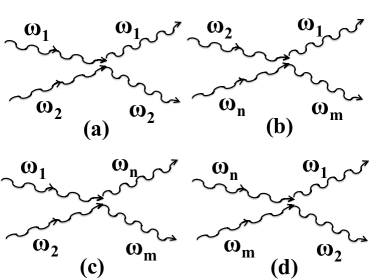
Figure 3: Depiction of scattering events coupling modes 1 and 2.

For a two-mode theory with $n^{\prime}=m=1$ and $n=m^{\prime}=2$ we obtain the off-diagonal non-linear frequency shift of Muduli, Heinonen, and ÅkermanMuduli et al. (2012) [Fig. 3 (a)]. Scattering processes such as the one depicted in Fig. 3 (b) will give rise to linear terms of the form $dA_{1}(t)/dt\propto BA_{2}(t)$, with $B$ some constant, provided $\omega_{1}+\omega_{m}=\omega_{2}+\omega_{n}$, or stated differently, provided $\omega_{2}-\omega_{1}=\omega_{m}-\omega_{n}$, can be satisfied, and (ii) mode $n$ is occupied. The latter condition is generally satisfied at finite temperatures due to thermal occupation. The former can in general be satisfied because firstly, the magnon energies are small compared to room temperature or elevated temperatures in the STOs because of Joule heating. Therefore, modes in a very large portion of the magnon spectrum are thermally occupied. Secondly, there will then be magnon modes $m$ and $n$ somewhere in the thermally occupied part of the spectrum such that the energy conservation requirement $\omega_{2}-\omega_{1}=\omega_{m}-\omega_{n}$ can be satisfied as the spacing between magnon frequencies is not uniform. The possible contributions to this kind of linear coupling also increase with increasing order in $c_{i}$. For example, in fifth order incoming modes $\omega_{2}$ and $\omega_{n}$ can scatter into modes $\omega_{1}$, $\omega_{m}$, $\omega_{m^{\prime}}$ and $\omega_{m^{\prime\prime}}$, provided $\omega_{2}+\omega_{n}=\omega_{1}+\omega_{m}+\omega_{m^{\prime}}+\omega_{m^{\prime\prime}}$. The contributions to this linear coupling also increases as a mode crossing is approached so that $\omega_{1}\to\omega_{2}$, in which case $\omega_{m}\to\omega_{n}$ and energy conservation is satisfied for any mode $\omega_{n}$. Other possible scattering events coupling modes 1 and 2 are depicted in Fig. 3 (c) and (d), but the contributions from such events are zero because under the assumptions that modes 1 and 2 have the lowest frequencies, these events cannot satisfy energy conservation at the vertex. Similarly, the second sum in Eq. (38) correspond to one incoming mode and three outgoing modes at the vertex for which energy can not be conserved at the vertex with $n^{\prime}=1$ (2) and $n=2$ (1).

The terms in $c_{i}^{2}$ in Eq. (37) give rise to contributions of the form

$$\sum_{n,m,m^{\prime}}A_{n}A_{m}A_{m^{\prime}}{\rm e}^{-i(\omega_{n}+\omega_{m}+\omega_{m^{\prime}}-\omega_{n^{\prime}})t}\pm\sum_{n,m,m^{\prime}}A_{n}^{*}A_{m}A_{m^{\prime}}{\rm e}^{-i(-\omega_{n}+\omega_{m}+\omega_{m^{\prime}}-\omega_{n^{\prime}})t},$$ (39)

which, after integrating over time, will give rise to non-zero terms provided $\omega_{n}+\omega_{m}+\omega_{m^{\prime}}-\omega_{n^{\prime}}=0$, or $-\omega_{n}+\omega_{m}+\omega_{m^{\prime}}-\omega_{n^{\prime}}=0$. The former cannot be satisfied for events coupling modes 1 and 2 since there are three incoming modes, two of which have higher frequencies than modes 1 or 2. The second sum in Eq. (39) gives rise to the same kind of terms as the first sum in Eq. (38).

For an effective two-mode theory with modes 1 and 2 dominant, the diagonal and off-diagonal nonlinear frequency shifts of mode 1 are given by

$$-\frac{i}{4}A_{1}|A_{1}|^{2}\sum_{i,i^{\prime}}\left(D_{i,i^{\prime};yy}+D_{i,i^{\prime};zz}\right)d_{i,1}^{*}d_{i^{\prime},1}|d_{i^{\prime},1}|^{2}$$

$$-\frac{i}{2}A_{1}|A_{1}|^{2}\sum_{i,i^{\prime}}\left(D_{i,i^{\prime};yy}+D_{i,i^{\prime};zz}\right)d_{i,1}^{*}d_{i^{\prime},1}|d_{i,1}|^{2}$$

$$-\frac{i}{4}A_{1}|A_{1}|^{2}\sum_{i,i^{\prime}}\left(D_{i,i^{\prime};yy}-D_{i,i^{\prime};zz}\right)d_{i,1}^{*}d_{i^{\prime},1}^{*}d_{i,1}^{2}$$

$$+2iA_{1}|A_{1}|^{2}\sum_{i,i^{\prime}}D_{i,i^{\prime};xx}d_{i,1}^{*}d_{i^{\prime},1}|d_{i^{\prime},1}|^{2}$$

$$-\frac{i}{4}A_{1}|A_{2}|^{2}\sum_{i,i^{\prime}}\left(D_{i,i^{\prime};yy}+D_{i,i^{\prime};zz}\right)d_{i,1}^{*}d_{i^{\prime},1}|d_{i^{\prime},2}|^{2}$$

$$-\frac{i}{2}A_{1}|A_{2}|^{2}\sum_{i,i^{\prime}}\left(D_{i,i^{\prime};yy}+D_{i,i^{\prime};zz}\right)d_{i,1}^{*}d_{i^{\prime},1}|d_{i,2}|^{2}$$

$$-\frac{i}{4}A_{1}|A_{2}|^{2}\sum_{i,i^{\prime}}\left(D_{i,i^{\prime};yy}-D_{i,i^{\prime};zz}\right)d_{i,1}^{*}d_{i^{\prime},1}^{*}|d_{i,2}|^{2}$$

$$+2iA_{1}|A_{2}|^{2}\sum_{i,i^{\prime}}D_{i,i^{\prime};xx}|d_{i,1}|^{2}|d_{i^{\prime},2}|^{2}$$ (40)

We can write Eq. (40) symbolically as

$$\frac{dA_{1}(t)}{dt}=-i\left[\omega_{1}\eta_{1,1}|A_{1}|^{2}+\omega_{2}|A_{2}|^{2}\right]A_{1},$$ (41)

with a similar equation for $dA_{2}(t)/(dt)$.

The other modes $n$ and $m$ constitute a bath of thermally populated modes. For the case $\omega_{n}+\omega_{2}-\omega_{m}-\omega_{1}=0$ we get ”back-scattering” terms of the form

$$\frac{dA_{1}(t)}{dt} = -\frac{i}{4}A_{2}\sum_{i,i^{\prime},m,n}d^{*}_{i,1}d_{i^{\prime},n}D_{i,i^{\prime};yy}A_{n}A^{*}_{m}d^{*}_{i^{\prime},m}d_{i^{\prime},2}$$ (42)

$$-2\frac{i}{4}A_{2}\sum_{i,i^{\prime},m,n}d^{*}_{i,1}d_{i,n}D_{i,i^{\prime};yy}A_{n}A^{*}_{m}d^{*}_{i,m}d_{i^{\prime},2}$$

$$-\frac{i}{4}A_{2}\sum_{i,i^{\prime},m,n}d^{*}_{i,1}d_{i^{\prime},n}D_{i,i^{\prime};zz}A_{n}A^{*}_{m}d^{*}_{i^{\prime},m}d_{i^{\prime},2}$$

$$-2\frac{i}{4}A_{2}\sum_{i,i^{\prime},m,n}d^{*}_{i,1}d_{i,n}D_{i,i^{\prime};zz}A_{n}A^{*}_{m}d^{*}_{i,m}d_{i^{\prime},2}$$

$$= -\frac{i}{4}A_{2}\sum_{i,i^{\prime},m,n}d^{*}_{i,1}d_{i^{\prime},n}D_{i,i^{\prime};yy}n_{B}(\omega_{n})d^{*}_{i^{\prime},m}d_{i^{\prime},2}$$

$$-2\frac{i}{4}A_{2}\sum_{i,i^{\prime},m,n}d^{*}_{i,1}d_{i,n}D_{i,i^{\prime};yy}n_{B}(\omega_{n})d^{*}_{i,m}d_{i^{\prime},2}$$

$$-\frac{i}{4}A_{2}\sum_{i,i^{\prime},m,n}d^{*}_{i,1}d_{i^{\prime},n}D_{i,i^{\prime};zz}n_{B}(\omega_{n})d^{*}_{i^{\prime},m}d_{i^{\prime},2}$$

$$-2\frac{i}{4}A_{2}\sum_{i,i^{\prime},m,n}d^{*}_{i,1}d_{i,n}D_{i,i^{\prime};zz}n_{B}(\omega_{n})d^{*}_{i,m}d_{i^{\prime},2},$$

where we have used the assumed thermal equilibrium of modes $m$ and $n$ to replace $A_{n}$ and $A^{*}_{m}$ with $n_{B}(\omega_{n})$ and unity, respectively, by taking a thermal average over magnon states. We note that both the nonlinear frequency shift as well as the linear ”back-scattering” term are driven by non-local nonlinear interactions inherent in the LLG equation.

V.3 Cubic non-conservative terms

Just like for the conservative terms, the expansion of $1/\sqrt{1-|c_{i}|^{2}}$ in the denominator and $\sqrt{1-|c_{i^{\prime}}|^{2}}$ in the field terms $H_{d,i^{\prime},y}$ and $H_{d.i^{\prime},z}$, together with the factors $|c_{i}|^{2}$ and $c_{i}^{2}$ will give rise to four-magnon vertex terms of the same structures as the conservative third-order terms and under the same conditions on the magnon frequencies. As these terms arise from the non-conservative torques, they will give rise to non-linear damping and pumping with both diagonal terms, as in the single-mode theory, and off-diagonal terms as in the two-mode description by Mudulu, Heinonen, and AkermanMuduli et al. (2012). Finally, there will also in an effective two-mode theory be a linear contribution of the form $dA_{1}(t)/dt\propto A_{2}(t)$ if there exist modes $m,n$ such that $\omega_{n}+\omega_{2}-\omega_{m}-\omega_{1}=0$. Again, this term can contribute only when there is a bath of thermally excited modes $n$.

With $\alpha=\alpha_{G}(1+q_{1}|c_{i}|^{2})$, the total cubic non-conservative terms are

$$\frac{\alpha_{G}}{4}\sum_{i^{\prime}}D_{i,i^{\prime};yy}\left(c_{i^{\prime}}+c_{i^{\prime}}^{*}\right)\left[3c_{i}^{2}-2|c_{i}|^{2}-|c_{i^{\prime}}|^{2}\right]$$

$$-\frac{\alpha_{G}}{4}\sum_{i^{\prime}}D_{i,i^{\prime};zz}\left(c_{i^{\prime}}-c_{i^{\prime}}^{*}\right)\left[3c_{i}^{2}+2|c_{i}|^{2}+|c_{i^{\prime}}|^{2}\right]$$

$$+2\alpha_{G}c_{i}\sum_{i^{\prime}}D_{i,i^{\prime};xx}\left[|c_{i}|^{2}-|c_{i^{\prime}}|^{2}\right]-a_{J}c_{i}|c_{i}|^{2}\cos\beta$$

$$+q_{1}\frac{\alpha_{G}}{2}\sum_{i^{\prime}}\left[\left(c_{i^{\prime}}+c_{i^{\prime}}^{*}\right)D_{i,i^{\prime};yy}+\left(c_{i^{\prime}}-c_{i^{\prime}}^{*}\right)D_{i,i^{\prime};zz}\right]|c_{i}|^{2}$$

$$-q_{1}\alpha_{G}c_{i}|c_{i}|^{2}\left(H_{\rm ext}-\overline{H}_{d,i,x}\right).$$ (43)

Again, for two dominant modes $1$ and $2$ we consider resonant scattering corresponding to Fig. 3 (a), and get the following contributions to the diagonal and off-diagonal non-linear damping and pumping:

$$\frac{\alpha_{G}}{2}A_{1}|A_{1}|^{2}\sum_{i,i^{\prime}}d_{i,1}^{*}d_{i^{\prime},1}|d_{i,1}|^{2}D_{i,i^{\prime};xx}$$

$$-\frac{\alpha_{G}}{4}A_{1}|A_{1}|^{2}\sum_{i,i^{\prime}}d_{i,1}^{*}d_{i^{\prime},1}|d_{i^{\prime},1}|^{2}\left[8D_{i,i^{\prime};xx}-D_{i,i^{\prime};yy}-D_{i,i^{\prime};zz}\right]$$

$$+\frac{\alpha_{G}}{4}A_{1}|A_{1}|^{2}\sum_{i,i^{\prime}}|d_{i,1}|^{2}d_{i^{\prime},1}^{*}d_{i,n}\left[3D_{i,i^{\prime};yy}+3D_{i,i^{\prime};zz}\right]$$

$$-q_{1}\alpha_{G}A_{1}|A_{1}|^{2}\sum_{i}|d_{i,1}|^{2}|d_{i,1}|^{2}\left(H_{\rm ext}-\overline{H}_{d,i,x}\right)-a_{J}\cos\beta A_{1}|A_{1}|^{2}\sum_{i}|d_{i,1}|^{2}|d_{i,1}|^{2}$$

$$+\frac{\alpha_{G}}{2}A_{1}|A_{2}|^{2}\sum_{i,i^{\prime}}d_{i,1}^{*}d_{i^{\prime},1}|d_{i,2}|^{2}D_{i,i^{\prime};xx}$$

$$-\frac{\alpha_{G}}{4}A_{1}|A_{2}|^{2}\sum_{i,i^{\prime}}d_{i,1}^{*}d_{i^{\prime},1}|d_{i^{\prime},2}|^{2}\left[8D_{i,i^{\prime};xx}-D_{i,i^{\prime};yy}-D_{i,i^{\prime};zz}\right]$$

$$+\frac{\alpha_{G}}{4}A_{1}|A_{2}|^{2}\sum_{i,i^{\prime}}d_{i,1}^{*}d_{i^{\prime},1}^{*}d_{i,2}^{2}\left[3D_{i,i^{\prime};yy}+3D_{i,i^{\prime};zz}\right]$$

$$-q_{1}\alpha_{G}A_{1}|A_{2}|^{2}\sum_{i}|d_{i,1}|^{2}|d_{i,2}|^{2}\left(H_{\rm ext}-\overline{H}_{d,i,x}\right)-a_{J}\cos\beta A_{1}|A_{2}|^{2}\sum_{i}|d_{i,1}|^{2}|d_{i,2}|^{2}$$ (44)

By considering scattering with thermally populated modes, as outlined earlier, we can also generate contributions to the ”back-scattering” terms analogous to Eq. (42), but we will not write these out here.

In the terms examined so far, linear non-conservative and cubic conservative and non-conservative terms, $a_{J}\cos\beta$ enters only as a product. As we indicated earlier, this implies that these equations are invariant under keeping $a_{J}\cos\theta$ constant, which can only explain an increase with threshold current with decreasing $\cos\beta$. It cannot explain any other behavior that changes with angle even if $a_{J}\cos\beta$ is held constant. Therefore, such angular dependence can only come from the terms in $a_{J}\sin\beta$ in Eq. (14).

We can combine the linear [Eq. (36)] and cubic nonconservative damping and pumping terms [Eq. (44)], and also the conservative and non-conservative ”back-scattering” terms in the following equation

$$\frac{dA_{1}(t)}{dt}=-\Gamma_{G}\left[1+P_{1,1}\omega_{1}|A_{1}|^{2}+P_{1,2}\omega_{2}|A_{2}|^{2}\right]A_{1}+\sigma_{0}I\cos\beta\left[1-Q_{1,1}\omega_{1}|A_{1}|^{2}-Q_{1,2}\omega_{2}|A_{2}|^{2}\right]A_{1}+R_{1,2}(T)A_{2},$$ (45)

with a similar equation for the nonlinear damping and pumping, and back-scattering, contributions to $dA_{2}(t)/(dt)$. We have noted the temperature dependence of the linear term that arises from scattering of thermally populated modes. In contrast with the nonlinear frequency shift, the non-linear damping and pumping is driven both by local (lines 5 and 8 in Eq. (44) as well as non-local terms; of course, the nonlinear damping originates in the magnetostatic interactions, just like the nonlinear frequency shift.

The thermal populations of modes $n$ and $m$ contributing to back-scattering terms arising from cubic terms have as a consequence that the backscattering terms will have a direct temperature dependence. As the backscattering terms are responsible for bifurcation and mode crossingBeri et al. (2008); van der Sande et al. (2008) this implies that the manifold of periodic orbits and fixed points, both stable and unstable ones at saddle points, will shift as the temperature is varied. This is in contrast to the temperature effects that occur when the system is coupled to a thermal bath that gives rise to a stochastic field. Thermal fluctuations will primarily induce mode-hopping over saddle points and thermal excursions around periodic orbits and stable fixed points, but have a small effect on the manifold itself.

V.4 $\sin\beta\not=0$

For $\sin\beta\not=0$, that is, when the fixed layer direction is not aligned with the equilibrium magnetization direction of the free layer, there arise new terms of different symmetry than what is otherwise the case: the terms in $\sin\beta$ are all in even powers of $|c_{i}|$ or $c_{i}$. This is in contrast with the other terms (both conservative and non-conservative ones), that all have odd powers in $c_{i}$ or $|c_{i^{\prime}}|$. Therefore, these terms in $\sin\beta$ cannot be canceled by the other conservative or non-conservative terms. As a consequence, new mode-mode scattering channels open up when the applied external field is rotated away from the direction of the fixed layer magnetization. Again, considering the two dominant modes 1 and 2, the lowest-order contributions from the terms in $c_{i}^{2}$ coupling modes 1 and 2 occur if $\omega_{2}+\omega_{m}=\omega_{1}$, or $\omega_{1}+\omega_{m}=\omega_{2}$, or $\omega_{1}+\omega_{2}=\omega_{m}$ is satisfied for some $m$. The first two of these are not allowed as $\omega_{m}>\omega_{2},\omega_{1}$, but the last represents the scattering of a magnon pair of modes 1 and 2 into mode $m$. Similarly the lowest-order term in $|c_{i}|^{2}$ only gives a non-zero contributions if $\omega_{m}=\omega_{2}+\omega_{1}$, which represents a decay of a thermally populated mode $m$ into modes 1 and 2. The available phase-space that satisfies the requirement $\omega_{m}=\omega_{2}+\omega_{1}$ for the possible three-magnon processes is at the most satisfied at special discrete values of an external control parameter, such as external field magnitude or direction, and will therefore be ignored here. Higher-order terms have larger available phase-space. In forth order, we have the terms

$$\frac{1}{8}a_{J}\sin[\beta]\left[|c_{i}|^{4}+c_{i}^{2}|c_{i}|^{2}\right].$$ (46)

We consider only contributions to $dA_{1}/(dt)$ which in diagrams of the type in Fig. 3 have at least one outgoing mode 1 magnon. Also, we only include scattering events that are compatible with $\omega_{m}>\omega_{1},\omega_{2}$ for all $m\not=1,2$. Finally, we exclude scattering events with only one magnon in the thermal bath as the requirement on energy conservation at the vertex can in general not be satisfied for such events. In all, we get the following contributions to $dA_{1}/(dt)$:

$$\frac{1}{8}a_{j}\sin[\beta] \left\{\sum_{m,n,i}A_{1}A_{2}n_{B}(\omega_{n})\delta(\omega_{n}+\omega_{2}-\omega_{m})|d_{i,1}|^{2}d_{i,2}d_{i,m}^{*}d_{i,n}\right.$$ (47)

$$\sum_{m,n,i}A_{2}^{2}n_{B}(\omega_{n})\delta(\omega_{n}+2\omega_{2}-\omega_{m}-\omega_{1})d_{i,1}^{*}d_{i,2}^{2}d_{i,m}^{*}d_{i,n}$$

$$\sum_{m,n,i}|A_{2}|^{2}n_{B}(\omega_{n})\delta(\omega_{n}-\omega_{m}-\omega_{1})d_{i,1}^{*}|d_{i,2}|^{2}d_{i,m}^{*}d_{i,n}$$

$$\sum_{m,n,i}A_{1}^{*}A_{2}n_{B}(\omega_{n})\delta(\omega_{n}+\omega_{2}-\omega_{m}-2\omega_{1}){d_{i,1}^{*}}^{2}d_{i,2}d_{i,m}^{*}d_{i,n}$$

$$\sum_{m,n,i}A_{1}^{2}n_{B}(\omega_{n})\delta(\omega_{n}+\omega_{1}-\omega_{m})|d_{i,1}|^{2}d_{i,1}d_{i,m}^{*}d_{i,n}$$

$$\left.\sum_{m,n,i}|A_{1}|^{2}n_{B}(\omega_{n})\delta(\omega_{n}-\omega_{1}-\omega_{m})|d_{i,1}|^{2}d_{i,1}^{*}d_{i,m}^{*}d_{i,n}\right\}.$$

These terms are more complicated than the ones we have considered previously in that they will not only couple the time evolution of $A_{1}$ and $A_{2}$ with linear terms or terms of the form of the non-linear damping or pumping, and their inclusion in an effective theory would require a much larger parameter set. We will not here further discuss such an effective theory as we are assuming that an expansion to third orded is sufficient, and therefore fourth-order terms multiplying $\sin\beta$ can certainly be ignored for small $\beta$. The main reason for discussing these terms is to point out that they alone can cause dependence on angle $\beta$ other than $a_{J}\cos\beta$ and are, for example, responsible for the observed increase in mode-hopping as $\cos\beta$ is decreased.

V.5 General equation for mode coupling

We can now collect all the terms up to and including third-order and write the coupled equations for modes 1 and 2 as

$$\frac{dA_{1}(t)}{dt} = -i\left[\omega_{1}\eta_{1,1}|A_{1}|^{2}+\omega_{2}\eta_{1,2}|A_{2}|^{2}\right]A_{1}$$ (48)

$$-\Gamma_{G}\left[1+P_{1,1}\omega_{1}|A_{1}|^{2}+P_{1,2}\omega_{2}|A_{2}|^{2}\right]A_{1}$$

$$+\sigma_{0}I\cos\beta\left[1-Q_{1,1}\omega_{1}|A_{1}|^{2}-Q_{1,2}\omega_{2}|A_{2}|^{2}\right]A_{1}+R_{1,2}(T)A_{2}$$

$$\frac{dA_{2}(t)}{dt} = -i\left[\omega_{1}\eta_{2,1}|A_{1}|^{2}+\omega_{2}\eta_{2,2}|A_{2}|^{2}\right]A_{2}$$ (49)

$$-\Gamma_{G}\left[1+P_{2,1}\omega_{1}|A_{1}|^{2}+P_{2,2}\omega_{2}|A_{2}|^{2}\right]A_{2}$$

$$+\sigma_{0}I\cos\beta\left[1-Q_{2,1}\omega_{1}|A_{1}|^{2}-Q_{2,2}\omega_{2}|A_{2}|^{2}\right]A_{2}+R_{2,1}(T)A_{1}$$

Equations (48) and (49) are the main result of the present work. They are the equations given by Muduli, Heinonen, and ÅkermanMuduli et al. (2012).

VI Summary and Conclusions

We have here presented detailed derivations of the equations of motions for coupled modes in STOs. In particular, we have shown that the equations governing a system with two dominant modes can be reduced to a set of coupled equations first given by Muduli, Heinonen, and ÅkermanMuduli et al. (2012), and are a generalization of the equations governing a single-mode STO, as given by Slavin and TiberkevichSlavin and Tiberkevich (2008, 2009). We have given explicit expressions for the linear terms and for the cubic terms responsible for nonlinear damping and pumping, as well as for the nonlinear frequency shift, for the geometries considered here. The linear ”back-scattering” term arise from scattering that is possible when there is a bath of modes available, and we have given explicit examples of such terms. In practice, these terms are difficult to calulate and the corresponding coefficients, $R_{1,2}$, and $R_{2,1}$, can probably be treated as parameters in modelingHeinonen et al. (2013). We have also concluded that these back-scattering terms have a direct temperature dependence as they involve thermal populations of modes. This implies that manifold of of orbit and fixed point will shift as a function of temperature, in addition to temperature effects, such as mode hopping, that may be the consequence of a stochastic field that arises from coupling to a thermal bath. The equations for the coupled modes include additional terms beyond third order that arise when the free layer equilibrium magnetization is not aligned with the fixed layer magnetization. These terms generate additional coupling between modes that provide a physical mechanism for observed increased mode-hopping as the external field is moved away from the direction of the fixed layer magnetization. The intrinsic nonlinear and non-local interactions in the LLG equation that governs the magnetization dynamics give rise to couplings between modes that in turn can generate a wealth of interesting complicated phenomena, such as mode-hopping or mode coexistence. These couplings and ensuing phenomena are of fundamental interest but also of significant importance for technological applications of STOs.

Yan Zhou acknowledges the support by the Seed Funding Program for Basic Research from the University of Hong Kong, and University Grants Committee of Hong Kong (Contract No. AoE/P-04/08). Argonne National Laboratory is operated under Contract No. DE-AC02-06CH11357 by UChicago Argonne, LLC. Comments by E. Iacocca are greatly appreciated.

APPENDIX

Here, we present the details of the derivation of Eq. (28) from Eq. (26). The linearized version of Eq. (26) is

$$\frac{dc}{dt}=-i\left(bc+nc^{*}\right),$$ (50)

where $b=H_{\rm ext}-X+\frac{1}{2}\left(Y+Z\right)$, and $n=\frac{1}{2}\left(Y-Z\right)$ with eigenvalue $\omega$ given by $\omega^{2}=b^{2}-n^{2}$. Equation (50) is diagonalized by introducing a complex variable $a$ such that $c=ua-va^{*}$ where $u=\sqrt{(b+\omega)/(2b)}$ and $v=\sqrt{(b-\omega)/(2b)}$. Thus $u$ and $v$ are real with $u^{2}+v^{2}=1$ and $u^{2}-v^{2}=\omega/b$. The variable $a$ is given in terms of $c$ by $a=(uc+vc^{*})/(u^{2}-v^{2})$. We multiply Eq.(26) by $u/(u^{2}-v^{2})$ and add from the result the complex conjugate of Eq. (26) multiplied by $v/(u^{2}-v^{2})$. The linear terms then become

$$\frac{da}{dt}=-i\omega a\left(1-i\alpha\right)$$ (51)

To work out the rest, we need

$$|c|^{2} = |a|^{2}-\frac{n}{2b}\left(a^{2}+{a^{*}}^{2}\right)$$ (52)

$$c^{2} = \frac{b+\omega}{2b}{a}^{2}+\frac{b-\omega}{2b}{a}^{*2}-\frac{n}{b}|a|^{2}$$ (53)

$${c^{*}}^{2} = \frac{b+\omega}{2b}{{a}*}^{2}+\frac{b-\omega}{2b}a^{2}-\frac{n}{b}|a|^{2}$$ (54)

$$\frac{uc-vc^{*}}{u^{2}-v^{2}} = \frac{b}{\omega}a-\frac{n}{\omega}a^{*}.$$ (55)

The most tedious part is the second line of Eq. (26), which is

$$-\frac{i}{2}\left(3H_{\rm ext}+X\right)c|c|^{2}+\frac{i}{4}\left(Y-Z\right)c^{3}+\frac{i}{4}\left(Y+Z\right)c|c|^{2}=-iAc|c|^{2}+\frac{i}{2}nc^{3},$$ (56)

where $A=\frac{1}{2}\left(3H_{\rm ext}+X\right)-\frac{1}{2}(Y+Z)$. We therefore need to evaluate

$$-iA\frac{u}{u^{2}-v^{2}}c|c|^{2}+iA\frac{v}{u^{2}-v^{2}}c^{*}|c|^{2}+\frac{1}{2}\frac{inu}{u^{2}-v^{2}}c^{3}-\frac{1}{2}\frac{inv}{u^{2}-v^{2}}{c^{*}}^{3}.$$ (57)

Using Eqs. (52) and (55), we obtain

$$\frac{uc-vc^{*}}{u^{2}-v^{2}}|c|^{2}=\frac{2b^{2}+n^{2}}{2b\omega}a|a|^{2}+\frac{3n}{2\omega}{a}^{*}|{a}|^{2}-\frac{n}{2\omega}a^{3}+\frac{n^{2}}{2b\omega}{a}^{*3}.$$ (58)

From Eqs. (53-55) we obtain

$$\frac{nuc}{u^{2}-v^{2}}c^{2}-\frac{nvc^{*}}{u^{2}-v^{2}}{c^{*}}^{2}=\frac{3}{2}\frac{n^{3}}{b\omega}{a^{*}}|a|^{2}-\frac{3}{2}\frac{bn^{2}}{b\omega}a|a|^{2}+\frac{1}{2}\frac{n(b^{2}+\omega^{2})}{b\omega}a^{3}-\frac{1}{2}\frac{n^{2}b}{b\omega}{a}^{*3}.$$ (59)

and also

$$\frac{u}{u^{2}-v^{2}}c^{3}+\frac{v}{u^{2}-v^{2}}{c^{*}}^{3}=a^{3}+\frac{n}{2b}{a}^{*3}-\frac{3n}{2b}a|a|^{2}.$$ (60)

Putting it all together, we get

$$\frac{da}{dt} = -i\omega a\left[1-i\alpha\right]+\frac{3i\omega}{2}a\left[|a|^{2}-\frac{n}{2b}\left(a^{2}+{a^{*}}^{2}\right)\right][1-i\alpha]$$ (61)

$$-iA\left[\frac{2b^{2}+n^{2}}{2b\omega}a|a|^{2}-\frac{3n}{2\omega}a^{*}|a|^{2}-\frac{n}{2\omega}a^{3}+\frac{n^{2}}{2b\omega}{a}^{*3}\right]$$

$$+\frac{in}{2}\left[\frac{3n^{2}}{2b\omega}a^{*}|a|^{2}-\frac{3n}{2\omega}a|a|^{2}+\frac{b^{2}+\omega^{2}}{2b\omega}a^{3}-\frac{n}{2b\omega}{a}^{*3}\right]$$

$$-\frac{\alpha}{2}\left[H_{\rm ext}+3X-3m\right]\left[a|a|^{2}-\frac{n}{2b}\left(a^{3}+a^{*}|a|^{2}\right)\right]$$

$$+\frac{3\alpha n}{2}\left[a^{3}+\frac{n}{2b}{a}^{*3}-\frac{3n}{2b}a|a|^{2}.\right]$$

$$+\frac{a_{J}}{2}\frac{b}{\omega}\sin\beta\sqrt{\frac{b+n}{b}}\left[1+\frac{3n-2b}{2b}|a|^{2}+\frac{5n-6b}{4b}a^{2}-\frac{n}{4b}{a}^{*2}\right]$$

$$+a_{J}\cos\beta a\left[1-|a|^{2}+\frac{n}{2b}\left(a^{2}-{a^{*}}^{2}\right)\right].$$

References

• Slonczewski (1996) J. C. Slonczewski, J. Magn. Magn. Mater. 159, L1 (1996).
• Berger (1996) L. Berger, Phys. Rev. B 54, 9353 (1996).
• Ralph and Stiles (2008) D. C. Ralph and M. D. Stiles, J. Magn. Magn. Mater. 320, 1190 (2008).
• Nazarov et al. (2008) A. V. Nazarov, K. Nikolaev, Z. Gao, H. Cho, and D. Song, J. Appl. Phys. 103, 07A503 (2008).
• Deac et al. (2008) A. M. Deac, A. Fukushima, H. Kubota, H. Maehara, Y. Suzuki, S. Yuasa, Y. Nagamine, K. Tsunekawa, D. D. Djayaprawira, and N. Watanabe, Nat. Phys. 4, 803 (2008).
• Houssameddine et al. (2009) D. Houssameddine, U. Ebels, B. Dieny, K. Garello, J.-P. Michel, B. Delaet, B. Viala, M.-C. Cyrille, J. A. Katine, and D. Mauri, Phys. Rev. Lett. 102, 257202 (2009).
• Zeng et al. (2010) Z. Zeng, K. H. Cheung, H. W. Jiang, I. N. Krivorotov, J. A. Katine, V. Tiberkevich, and A. Slavin, Phys. Rev. B 82, 100410 (2010).
• Muduli et al. (2012) P. Muduli, O. Heinonen, and J. Åkerman, Phys. Rev. B 86, 174408 (2012).
• Mancoff et al. (2006) F. B. Mancoff, N. D. Rizzo, B. N. Engel, and S. Tehrani, Appl. Phys. Lett. 88, 112507 (2006).
• Rippard et al. (2004) W. Rippard, M. Pufall, S. Kaka, S. Russek, and T. Silva, Phys. Rev. Lett. 92, 027201 (2004).
• Silva and Rippard (2008) T. J. Silva and W. H. Rippard, J. Magn. Magn. Mater. 320, 1260 (2008).
• Slavin and Tiberkevich (2008) A. Slavin and V. Tiberkevich, IEEE Trans. Magn. 44, 1916 (2008).
• Tiberkevich et al. (2008) V. S. Tiberkevich, A. N. Slavin, and J.-V. Kim, Phys. Rev. B 78, 092401 (2008).
• Kim et al. (2008) J.-V. Kim, V. Tiberkevich, and A. N. Slavin, Phys. Rev. Lett. 100, 017207 (2008).
• Slavin and Tiberkevich (2009) A. Slavin and V. Tiberkevich, IEEE Trans. Magn. 45, 1875 (2009).
• Berkov and Gorn (2007) D. V. Berkov and N. L. Gorn, Phys. Rev. B 76, 144414 (2007).
• Bonetti et al. (2012) S. Bonetti, V. Puliafito, G. Consolo, V. S. Tiberkevich, A. N. Slavin, and J. Åkerman, Phys. Rev. B 85, 174427 (2012).
• Bonetti et al. (2010) S. Bonetti, V. Tiberkevich, G. Consolo, G. Finocchio, P. Muduli, F. Mancoff, A. Slavin, and J. Åkerman, Phys. Rev. Lett. 105, 217204 (2010).
• Krivorotov et al. (2008) I. N. Krivorotov, N. C. Emley, R. A. Buhrman, and D. C. Ralph, Phys. Rev. B 77, 054440 (2008).
• Lee et al. (2004) K. J. Lee, A. Deac, O. Redon, J. Nozières, and B. Dieny, Nat. Mater. 3, 877 (2004).
• Sankey et al. (2005) J. C. Sankey, I. N. Krivorotov, S. I. Kiselev, P. M. Braganca, N. C. Emley, R. A. Buhrman, and D. C. Ralph, Phys. Rev. B 72, 224427 (2005).
• Muduli et al. (2012) P. K. Muduli, O. G. Heinonen, and J. Åkerman, Phys. Rev. Lett. 108, 207203 (2012).
• Dumas et al. (2013) R. Dumas, E. Iacocca, S. Bonetti, S. Sani, S. Mohseni, A. Eklund, J. Persson, O. Heinonen, and J. Åkerman, Phys. Rev. Lett. 110, 257202 (2013).
• Heinonen et al. (2013) O. Heinonen, P. Muduli, E. Iacocca, and J. Åkerman, IEEE Trans. Magn. 49, 4398 (2013).
• van der Sande et al. (2008) G. van der Sande, L. Gelens, P. Tassin, and J. Scirè, A. aand Danckaert, J. Phys. B: At. Mol. Opt. Phys. 41, 095402 (2008).
• Beri et al. (2008) S. Beri, L. Gelens, M. Mestre, G. van der Sande, G. Verschaffelt, G. Scirè, G. Mezosi, M. Sorel, and J. Danckaert, Phys. Rev. Lett. 101, 093903 (2008).
• Zhang et al. (2002) S. Zhang, P. M. Levy, and A. Fert, Phys. Rev. Lett. 88, 236601 (2002).
• Muduli et al. (2011) P. K. Muduli, O. G. Heinonen, and J. Åkerman, Phys. Rev. B 83, 184410 (2011).
• Li and Zhang (2003) Z. Li and S. Zhang, Phys. Rev. B 68, 024404 (2003).
• Sorel et al. (2002) M. Sorel, J. Laybourn, A. Scirè, S. Balle, G. Giuliani, R. Miglierina, and S. Donati, Opt. Lett. 27, 1992 (2002).
• Sorel et al. (2003) M. Sorel, G. Giuliani, A. Scirè, R. Miglierina, J. Laybourn, and S. Donati, IEEE J. Quantum Electron. 39, 1187 (2003).