THE RADIO RELICS AND HALO OF EL GORDO, A MASSIVE $z=0.870$ CLUSTER MERGER

Abstract

We present $610\,\rm MHz$ and $2.1\,\rm GHz$ imaging of the massive Sunyaev Zel’dovich Effect (SZE)-selected $z=0.870$ cluster merger ACT-CL J0102-4915 (“El Gordo”), obtained with the Giant Metre-wave Radio Telescope (GMRT) and the Australia Telescope Compact Array (ATCA), respectively. We detect two complexes of radio relics separated by $3.4^{\prime}$ ($1.6\,\rm Mpc$) along the system’s northwest-to-southeast collision axis that have high integrated polarization fractions ($33\%$) and steep spectral indices ($\alpha$ between 1–2; $S_{\nu}\propto\nu^{-\alpha}$), consistent with creation via Fermi acceleration by shocks in the intracluster medium triggered by the cluster collision. From the spectral index of the relics, we compute a Mach number $\mathcal{M}=2.5^{+0.7}_{-0.3}$ and shock speed of $2500^{+400}_{-300}\,\rm km\,s^{-1}$. With our wide-bandwidth, full-polarization ATCA data, we compute the Faraday depth $\phi$ across the northwest relic and find a range of values spanning $\Delta\phi=30\,\rm rad\,m^{-2}$, with a mean value of $\left<\phi\right>=11\,\rm rad\,m^{-2}$ and standard deviation $\sigma_{\phi}=6\,\rm rad\,m^{-2}$. With the integrated line-of-sight gas density derived from new Chandra X-ray observations, our Faraday depth measurement implies $B_{\parallel}\sim 0.01\,\rm\mu G$ in the cluster outskirts. The extremely narrow shock widths in the relics ($d_{\rm shock}\leq 23\,\rm kpc$), caused by the short synchrotron cooling timescale of relativistic electrons at $z=0.870$, prevent us from placing a meaningful constraint on the magnetic field strength $B$ using cooling time arguments. In addition to the relics, we detect a large ($r_{\rm H}\simeq 1.1\,\rm Mpc$ radius), powerful ($\log(L_{1.4}/\rm W\,Hz^{-1})=25.66\pm 0.12$) radio halo with a shape similar to El Gordo’s “Bullet”-like X-ray morphology. The spatially-resolved spectral-index map of the halo shows the synchrotron spectrum is flattest near the relics, along the system’s collision axis, and in regions of high $T_{\rm gas}$, all locations associated with recent energy injection. The spatial and spectral correlation between the halo emission and cluster X-ray properties supports primary-electron processes like turbulent reacceleration as the halo production mechanism. The halo’s integrated $610\,\rm MHz$ to $2.1\,\rm GHz$ spectral index is a relatively flat $\alpha=1.2\pm 0.1$, consistent with the cluster’s high $T_{\rm gas}$ in view of previously established global scaling relations. El Gordo is the highest-redshift cluster known to host a radio halo and/or radio relics, and provides new constraints on the non-thermal physics in clusters at $z>0.6$.

1. Introduction

Galaxy clusters grow out of peaks in the primordial matter distribution of the early Universe and gain mass by accreting gas from their environments and by merging with other clusters and groups of galaxies. Because the physical properties and dynamical state of the intracluster medium (ICM) are affected by its merger history, observations of the ICM can be used to study the growth and evolution of clusters. Cluster mergers can inject large amounts of gravitational potential energy ($\sim 10^{64}\,\rm erg$) into the ICM, and observations of cluster-scale radio synchrotron emission, particularly in merging and dynamically disturbed systems (e.g., Buote, 2001; Pfrommer et al., 2008; Brunetti et al., 2009; Cassano et al., 2011), indicate that some fraction of this energy is directed into accelerating cosmic ray electrons to ultra-relativistic ($\gamma\sim 10^{3}$–$10^{4}$) energies. The resulting non-thermal radio emission is seen as a radio halo, i.e., diffuse axisymmetric emission centered on the cluster, or as radio relics, narrow, extended, filamentary structures located near the cluster outskirts (for reviews, see Ferrari et al. 2008 and Feretti et al. 2012).

Competing explanations for nonthermal relic and halo emission fall in two categories. “Primary” models rely on acceleration of electrons by shocks (e.g., first-order Fermi process: Ensslin et al. 1998) or turbulence (e.g., turbulent reacceleration process: Brunetti et al. 2001) in the ICM. “Secondary” models posit that cosmic-ray electrons are produced by inelastic hadronic collisions between thermal protons and cosmic ray protons, the latter accelerated by cluster mergers and long lived (Dennison, 1980). Because these models make different predictions about whether and how the strength and spectral shape of radio emission relate to the local state of the ICM, by studying the spectral, morphological, and polarization properties of radio halos and relics, we can probe the poorly understood non-thermal properties of galaxy clusters such as cosmic ray acceleration and magnetic field profiles. The geometry of relic systems can also be used to constrain the collision parameters of cluster mergers (van Weeren et al., 2011a).

One challenge in using relics and halos to probe the energy content and magnetic field properties of clusters is their relative rarity. Only $\simeq 30\%$ of X-ray luminous clusters host halos (Venturi et al., 2007, 2008). Their presence is correlated with cluster mass and dynamical state, with the most massive and most dynamically disturbed clusters showing the highest frequencies of halos and relics (Cassano et al., 2013; Sommer & Basu, 2014). Large radio relics, arcs with lengths $\geq 1\,\rm Mpc$, are found only in massive, merging clusters, and even rarer double-relic systems are found only in binary cluster mergers occurring in the plane of the sky.

The paucity of massive high-redshift clusters combined with the steep observed spectral index $\alpha$ of the non-thermal emission ($\alpha\simeq 1.5$; Ferrari et al., 2008) make the study of halos and relics at high redshifts especially difficult. Additionally, energy losses of the relativistic electrons to cosmic microwave background (CMB) photons through inverse Compton scattering are expected to reduce the radiative lifetimes, and therefore detectability, of synchrotron-emitting regions. Because of the above limitations, catalogs of known radio halo and relic clusters only extend to low redshifts; the highest-redshift halo cluster discovered to date is PLCK G147.3–16.6 ($z=0.65$; van Weeren et al., 2014). Nuza et al. (2012) predict that many more $z>0.3$ relics should exist than are currently catalogued, with the deficit likely due to lack of observations. To understand the nature of non-thermal emission in clusters throughout cosmic time, we need to increase the sample of known relics and halos at high redshift.

In this work, we present new $610\,\rm MHz$ and $2.1\,\rm GHz$ observations of the extremely massive, $z=0.870$ cluster ACT-CL J0102-4915 (also known as “El Gordo,” and hereafter referred to by that name; Menanteau et al., 2012), which reveal an associated radio halo and double radio relics. As the highest redshift radio-halo cluster now known, El Gordo can help fill in the gaps in our knowledge about non-thermal cluster physics at high redshift when the Universe was only half its current age. Section 2 describes El Gordo, Section 3 describes our observations and data reduction algorithms, Sections 4 and 5 present our analyses of and results for the relics and halo, respectively, and Section 6 presents our conclusions. In our calculations, we assume a nine-year $WMAP$ cosmology with $H_{0}=70\,\rm km\,s^{-1}\,Mpc^{-1}$, $\Omega_{M}=0.27$, and $\Omega_{\lambda}=0.73$ (Hinshaw et al., 2013). At $z=0.870$, $D_{\rm L}=5656\,\rm Mpc$, $D_{\rm A}=1618\,\rm Mpc$, and $1\rm\,arcmin$ corresponds to $0.47\rm\,Mpc$.

2. ACT-CL J0102-4915, “El Gordo”

El Gordo was discovered through its $148\,\rm GHz$ Sunyaev-Zel’dovich effect (SZE; Sunyaev & Zeldovich, 1972) decrement by the Atacama Cosmology Telescope (ACT; Fowler et al., 2007) collaboration. With a SZE centroid at $01^{\rm h}02^{\rm m}53^{\rm s}$ $-49^{\circ}15^{\prime}19^{\prime\prime}$ (J2000) and the strongest SZE signal in the $455\,\rm deg^{2}$ southern ACT survey (Marriage et al., 2011), El Gordo was optically confirmed as a bona fide galaxy cluster at $z=0.870$ (Menanteau et al., 2010) with a “bullet”-like merger morphology revealed in $Chandra$ X-ray imaging (Menanteau et al., 2012). El Gordo’s collision axis, identified by the system’s elongation in the X-ray surface brightness and the relative positions of two optical galaxy density peaks, lies in the northwest-to-southeast direction at a position angle of $136^{\circ}$ (Menanteau et al., 2012). Based on the merger morphology, Menanteau et al. (2012) predict the inclination angle $\phi$ (between the collision axis and the plane of the sky) to be shallow, in the range $\phi=15$–$30^{\circ}$. The cluster is also the most significant detection in the (overlapping) $2500\,\rm deg^{2}$ survey (Williamson et al., 2011) of the South Pole Telescope (SPT; Carlstrom et al., 2011). El Gordo has an observed-frame $0.5$–$2.0\,\rm keV$ X-ray luminosity of $L_{\rm X}=(2.19\pm 0.11)\times 10^{45}\,\rm erg\,s^{-1}$ and an integrated X-ray temperature of $k_{\rm B}T_{\rm gas}=14.5\pm 0.1\,\rm keV$ (Menanteau et al., 2012). By combining X-ray, SZE, and velocity dispersion measurements, Menanteau et al. (2012) estimate a total mass within $r_{500c}$, the radius containing 500 times the critical density of the universe, of $M_{500c}=(1.17\pm 0.17)\times 10^{15}\,M_{\odot}$. This mass estimate is compatible with subsequent analyses of strong lensing by Zitrin et al. (2013) and of weak lensing by Jee et al. (2013).

3. Observations and data reduction

3.1. 2.1 GHz ATCA

We used the Australia Telescope Compact Array (ATCA) to acquire 2.1GHz imaging of El Gordo. The Compact Array Broadband Backend (CABB; Wilson et al., 2011) has 2048 $1\,\rm MHz$-wide channels that span $1.1$–$3.1\,\rm GHz$. The observations were obtained in two installments (see Table 1): 12 hours in the extended 6A configuration in December 2011 (PI: Baker), and 8 hours in the compact 1.5B configuration in April 2012 (PI: Lindner). Calibration used the flat-spectrum, radio-loud quasars PKS 1934-638 (bandpass and flux calibration) and PKS 0047-579 (initial phase calibration). Observations of PKS 1934-638 bracketed each observing session, while phase-tracking observations of PKS 0047-579 were taken every 30 minutes. We used the software package MIRIAD (Sault et al., 1995) to calibrate, flag, invert, and clean the visibility data.

Radio frequency interference (RFI) is significant in the $2.1\,\rm GHz$ band at the ATCA. We removed RFI from the data both manually using the MIRIAD tasks pgflag and blflag, and automatically using the MIRIAD task mirflag (Middelberg, 2006). Baseline 1–2 ($uv$ distance $=194\,\lambda$) in the 2012 observations contained powerful broad-spectrum RFI and was entirely flagged. In total, 22% of visibilities were flagged. We used the task invert to produce multi-frequency synthesis (MFS) continuum images and mfclean to remove artifacts caused by the dirty beam and produce cleaned images. The data were then self-calibrated, first allowing the phase to vary, then phase and amplitude together. The final image was made with robust$=0$ $uv$ weighting, giving a synthesized beam with dimensions $6.1^{\prime\prime}\times 3.1^{\prime\prime}$ and a position angle ${\rm PA}=-1.9^{\circ}$. The image RMS noise at the phase center is $\sigma_{2.1}=8.2\,\rm\mu Jy\,beam^{-1}$ for an effective frequency of $\nu=2.15\,\rm GHz$. The $2.1\,\rm GHz$ map of El Gordo is shown in Figure 1.

The 2011 and 2012 observations have parallactic angle coverages of $120^{\circ}$ and $230^{\circ}$, respectively, allowing for polarization calibration. Schnitzeler et al. (2011) note that the instrumental polarization leakage across the CABB bandpass varies with frequency. Therefore, during gain calibration, we solved for leakage corrections separately in each of eight $256\,\rm MHz$-wide subbands using the gpcal option nfbin$=8$.

3.2. 610 MHz GMRT

We used the 30-antenna Giant Metre-wave Radio Telescope (GMRT) to acquire $610\,\rm MHz$ imaging of El Gordo. Observations were carried out in August 2012 (PI: Lindner) in three four-hour tracks. We used the quasar 3C48 for bandpass and flux calibration and J 0024-420 for initial phase calibration. The data have 256 130 kHz-wide channels for a total bandwidth of $33\,\rm MHz$ and an effective frequency of $607.7\,\rm MHz$. The $uv$ data were calibrated and imaged using the Common Astronomy Software Applications (CASA) package (Version 4.0.0). The tracks were visually inspected to remove powerful RFI spikes that were constant in either time or frequency, and transient RFI signals were removed using the automated flagging algorithm AOFLAGGER (Offringa et al., 2010, 2012).

The GMRT’s non-coplanar $uv$ dataset was imaged using three facets and 512 $w$-projection planes. The final self-calibrated map is shown in Figure 2 and has an RMS sensitivity of $\sigma_{610}=26\,\rm\mu Jy\,beam^{-1}$ and a synthesized beam of $11.0^{\prime\prime}\times 4.0^{\prime\prime}$ at position angle $-4.3^{\circ}$. The elongated synthesized beam is due to the low maximum elevation ($\simeq 20^{\circ}$) when El Gordo is observed from the GMRT site.

Our measured flux densities at $610\,\rm MHz$ and $2100\,\rm MHz$ are affected by both statistical image noise and systematic errors in the bootstrapped absolute flux densities of the flux calibrators. We have included this extra systematic error, 10% for GMRT (Baars et al., 1977; Chandra et al., 2004) and 5% for ATCA (Reynolds, 1994), in the quoted uncertainties for all measured flux densities and derived quantities.

4. Radio relics

Menanteau et al. (2012) identified two $843\,\rm MHz$ sources on opposite sides of El Gordo in archival data from the Sydney University Molonglo Sky Survey (SUMSS; Mauch et al., 2003) that were aligned with the collision axis and coincided with the locations of possibly shocked thermal gas, as traced by an unsharp-masked image of the $Chandra$ $0.5$–$2.0\,\rm keV$ X-ray map (Menanteau et al., 2012). This morphology is the signature arrangement of well-studied double radio relics in binary major cluster mergers at lower redshifts (e.g., van Weeren et al., 2011b). In this arrangement, the filamentary relics are spatially extended perpendicular to the system’s collision axis, identifying an outward-propagating shock front in the ICM. The outermost edges (with respect to the cluster center) of the radio relics correspond to the leading edges of the shock fronts. The trailing emission traces downstream shocked regions, which can be identified by their steeper spectral indices compared to the leading edges, caused by synchrotron spectral aging. The flattest spectral indices are thus found in the leading edges of the relics where recent energy injection has taken place. Our $2.1\,\rm GHz$ ATCA and $610\,\rm MHz$ GMRT maps confirm the presence of the relics in El Gordo, whose properties we detail below.

4.1. Geometries

The elongation directions of all relics are perpendicular to the collision axis (see Figures 1 and 2), suggesting the relics are created by shock waves in the ICM of the cluster merger (Ensslin et al., 1998). Our high-resolution imaging reveals the northwest SUMSS source to be an extended radio relic (hereafter referred to as the NW relic), which is resolved in both length and width by our observations. The NW relic has a total length of $1.2^{\prime}$ ($0.56\,\rm Mpc$), a thickness of $34^{\prime\prime}$ ($0.27\,\rm Mpc$), and a bright, unresolved ridge of emission on its northwest (outer) edge. The internal structure of the NW relic is complex; it contains a trailing filament with an unresolved width that is extended along a position angle offset from the NW relic’s leading edge. The flux from the southeast SUMSS source is due to a compact radio source (C10) with $S_{2.1\,\rm GHz}={(1.9\pm 0.1)\,\rm mJy}$ (see Table THE RADIO RELICS AND HALO OF EL GORDO, A MASSIVE $z=0.870$ CLUSTER MERGER), probably unrelated to the cluster, superposed on a much fainter extended component that we interpret as a likely radio relic (hereafter referred to as the SE relic). A third component of extended filamentary emission located $\sim 1^{\prime}$ northeast of the SE relic we will refer to as the E relic; it has a resolved length of $71^{\prime\prime}$ ($0.27\,\rm Mpc$). The widths of the E and SE relics and the width of the bright leading edge of the NW relic are all unresolved by our observations, indicating very narrow shocked regions of $d_{\rm shock}\leq 23\,\rm kpc$ (Figure 1).

To study the photometric properties of the SE relic, we subtract C10 from the image data by modelling its emission as a collection of elliptical Gaussian sources. We find that three Gaussian components are sufficient to produce residuals consistent with noise. Figure 3 displays the best-fit model configuration, which consists of a dominant source whose shape is consistent with the synthesized beam (“A”), a moderate flux density, resolved component closely associated with the point source (“B”), and a faint very extended component elongated perpendicular to El Gordo’s collision axis (“C”). Our subsequent photometric analysis of the relics is performed in images with components “A” and “B” subtracted out. Table THE RADIO RELICS AND HALO OF EL GORDO, A MASSIVE $z=0.870$ CLUSTER MERGER lists the integrated photometric properties of the relics.

Figure 4 presents a profile of the NW relic projected perpendicular to the collision axis, showing the leading unresolved edge followed by an extended trail of low-level signal likely caused by the spherical projection of a 3D shock structure and filamentary substructures in the shock material. Similar extended tails are seen in simulations of cluster mergers by van Weeren et al. (2011a).

4.2. Spectral indices

Our multi-wavelength data allow us to produce a $610\,\rm MHz$/$2.1\,\rm GHz$ spectral index ($\alpha^{2.1}_{0.6}$) map using the full GMRT and ATCA images, and a $1.6\,\rm GHz$/$2.6\,\rm GHz$ spectral index ($\alpha^{2.6}_{1.6}$) map using the upper and lower halves (i.e., $1.1-2.1\,\rm GHz$ and $2.1-3.1\,\rm GHz$) of the ATCA bandpass. We need not worry about incomplete recovery of large-scale emission in the relics because even the largest dimension of the NW relic ($1.3^{\prime}$) is smaller than the angular scale on which we expect our ATCA data to begin resolving out emission ($\gtrsim 1.9^{\prime}$) given the minimum $uv$ distance ($1.8\,\rm k\lambda$) at the high-frequency end of the bandpass. The GMRT data extend to a lower $uv$ distance and preserve emission on scales even larger than the cluster. Each pair of images was smoothed to a common circular beam ($11^{\prime\prime}$ for $\alpha_{0.6}^{2.1}$ and $8^{\prime\prime}$ for $\alpha^{2.6}_{1.6}$) and then clipped at a $4\sigma$ level before we computed the spectral index $\alpha$.

Figures 5 and 6 present the $\alpha^{2.1}_{0.6}$ and $\alpha^{2.6}_{1.6}$ spectral index maps of the NW relic, respectively. The integrated spectral indices are $\alpha^{2.1}_{0.6}=1.19\pm 0.09$ and $\alpha^{2.6}_{1.6}=2.0\pm 0.2$. Figures 7 and 8 show $\alpha^{2.1}_{0.6}$ and $\alpha^{2.6}_{1.6}$ for the the E and SE relics, respectively. The E relic has integrated spectral index values of $\alpha^{2.1}_{0.6}=0.9\pm 0.1$ and $\alpha^{2.6}_{1.6}=1.2\pm 0.5$, and the SE relic spectral indices are $\alpha^{2.1}_{0.6}=1.4\pm 0.1$ and $\alpha^{2.6}_{1.6}=1.2\pm 0.4$.

For the NW and E relics, where unlike the SE relic there are no uncertainties in the flux due to contamination by a nearby radio source, $\alpha^{2.6}_{1.6}$ is steeper than $\alpha^{2.1}_{0.6}$ due to spectral aging effects at high frequencies. The E relic resembles the leading edge of the NW relic in its narrow width and flatter spectral index, which are likely due to decreased projection effects and recent energy injection.

4.3. Rotation measure and $B_{\parallel}$

Magnetized plasma along the line of sight to polarized emission will cause Faraday rotation of the polarization angle of the emitted photons by an amount $\Delta\Psi\;[\rm rad]={\rm RM}\times\lambda^{2}$, where $\Psi$ is the polarization angle ($\Psi=0.5\tan^{-1}(U/Q)$), $\lambda\;[\rm m]$ is the wavelength of observation, and $\rm RM\;[rad\,m^{-2}]$ is the rotation measure. Our wide-bandwidth, full-polarization ATCA data allow us to measure the RM of the relic signal and constrain the integrated product of the parallel component of the magnetic field $B_{\parallel}$ and the free electron density $n_{e}$ through the cluster outskirts at a projected cluster-centric distance of $871\,\rm kpc$. For a single source of polarized emission, the rotation measure is equal to the Faraday depth ${\rm\phi}\,[{\rm rad\,m^{-2}}]=0.81\,\int_{\rm source}^{\rm observer}n_{e}B_{\parallel}dl$ (Burn, 1966), with $B_{\parallel}$ in $\rm\mu G$, $n_{e}$ in $\rm cm^{-3}$, and $dl$ in $\rm pc$. To avoid “$n\pi$” errors and to allow for the detection of multiple RM components, we compute the Faraday spectrum, the complex polarized surface brightness per unit Faraday depth $F(\phi)$ $[\rm Jy\,beam^{-1}\,\phi^{-1}]$, using the RM synthesis algorithm (Brentjens & de Bruyn, 2005) as implemented by the Astronomical Image Processing System (AIPS) in the task FARS.

We first produced $10\,\rm MHz$-wide $Q$ and $U$ images with $3^{\prime\prime}$ pixels, which were then individually corrected for the varying primary beam attenuation across the wide CABB bandwidth, smoothed to a common resolution with a circular synthesized beam of FWHM $11^{\prime\prime}$, and assembled into a single data cube before we ran FARS. The region of maximum sensitivity is a circle with radius $\sim 14^{\prime}$, entirely covering the cluster, which is set by the high-frequency end of the bandpass. The $10\,\rm MHz$-wide channel maps were then weighted by the inverse variance of the noise within a central $8^{\prime}$ box. The effective $\left<\lambda^{2}\right>$ of the data is $\left<\lambda^{2}\right>=0.20\,\rm m^{2}$. The FWHM of the RM transfer function (RMTF), shown in Figure 9, is $\delta_{\rm RM}=145\,\rm rad\,m^{-2}$.

The spatially-integrated Faraday depth spectrum for the polarized emission in the NW relic is shown in Figure 10. We find that the polarized signal in each pixel is consistent with a single, dominant Faraday component. Therefore, the polarized emission from the NW relic is likely originating from a single plane behind the magnetized plasma of the cluster and foreground material. We find no other significant Faraday components out to $\pm 10^{4}\,\rm rad\,m^{-2}$. We next used the AIPS task AFARS to produce an image showing the Faraday depth of the dominant component in each pixel across the relic (Figure 11). The Faraday depth contribution from the Galaxy is estimated using the RM maps of Oppermann et al. (2012). Within a $2^{\circ}$-radius circle centered on El Gordo, the mean Galactic RM value is $1.0\,\rm rad\,m^{-2}$, with a range between $-0.1\,\rm rad\,m^{-2}$ and $+1.9\,\rm rad\,m^{-2}$.

The Faraday depths for the NW relic have a Galactic-subtracted mean of $\left<\phi\right>=11\,\rm rad\,m^{-2}$ and a standard deviation of $\sigma_{\phi}=6\,\rm rad\,m^{-2}$; across the relic they span a range from $-5\,\rm rad\,m^{-2}$ to $+25\,\rm rad\,m^{-2}$. The uncertainty in each Faraday depth value is given by $\delta_{\rm RM}/(2\times{\rm SNR})$, where SNR is the signal-to-noise ratio in the Faraday spectrum. For the pixels shown in Figure 11, the uncertainties range between 5–$10\,\rm rad\,m^{-2}$. The Faraday depths of the NW relic are similar to the RM values of the radio relics in the Coma cluster presented recently by Bonafede et al. (2013), who find a mean value $\left<{\rm RM}\right>=14\,\rm rad\,m^{-2}$ with $\left<\sigma_{\rm RM}\right>=17\,\rm rad\,m^{-2}$. For a system which only has a single Faraday component we would expect consistency between RM and Faraday depth measurements, although we note that RM measurements derived using $d\Psi/d\lambda^{2}$ with sparse $\lambda^{2}$ coverage (e.g., Bonafede et al., 2013) are subject to greater systematic uncertainties than Faraday depth measurements derived using RM synthesis. We find that the range of Faraday depths across the NW relic significantly exceeds that due to the RMTF, likely reflecting the changing magnetic field strength and orientation ($\int B_{\parallel}\,dl$) in the ICM. Bonafede et al. (2013) also find significant variations in RM across the Coma relics and suggest they are due to turbulence in the ICM.

Recently, O’Sullivan et al. (2012) studied the Faraday spectra of four bright ($>1\,\rm Jy$) radio-loud active galactic nuclei using the ATCA/CABB at $2.1\,\rm GHz$ and obtained RMTF widths $\delta_{\rm RM}\simeq 60\,\rm rad\,m^{-2}$, i.e., narrower than ours. The reason for this difference in $\delta_{\rm RM}$ is our goal of detecting the $<1\,\rm mJy$ polarized emission from faint relic structure in El Gordo, which leaves us more susceptible to low-level RFI. RFI generally increases at low frequencies, thereby reducing the weights of the high-$\lambda^{2}$ coverage and increasing the width of the RMTF, given by $\delta_{\rm RM}=2\sqrt{3}/(\lambda^{2}_{\rm max}-\lambda^{2}_{\rm min})$. We note that when we use equal weighting instead of inverse-variance weighting across the $\lambda^{2}$ channels, our RMTF becomes significantly narrower with $\delta_{\rm RM}=79\,\rm rad\,m^{-2}$, although the RM centroid uncertainties $\sigma_{\rm RM}$ are not improved in this case due to the increased noise from including all low-frequency channels.

The electron column density along the line-of-sight to the NW relic is computed by integrating the cylindrically-deprojected electron density model from Menanteau et al. (2012) from the cluster mid-plane out to infinity, and is $\int n_{e}\,dl=954\,\rm cm^{-3}\,pc$. We thus estimate the mean value for the parallel component of the magnetic field as $\left<B_{\parallel}\right>=\left<\phi\right>/(0.81\int n_{e}\,dl)$, and find $B_{\parallel}\sim 0.01\,\rm\mu G$ in the outskirts of El Gordo. Caution should be used when interpreting the above magnetic field strength due to the significant assumption (necessary given the lack of knowledge about the magnetic field’s topology) that the projected magnetic field strength is constant along the line of sight.

4.4. Polarization

Highly polarized synchrotron emission is evidence of a highly aligned magnetic field in an emitting region. Such alignment can be caused by shocks sweeping up ICM material at the locations of radio relics. The total amplitude of linearly polarized emission $P=\sqrt{Q^{2}+U^{2}}$, and the total fractional polarization is given by $f_{P}=P/I$. Uncertainties in $P$ and $f_{P}$ follow a Rice distribution, which has non-zero mean. In our maps, we account for this bias by multiplying the polarized signal $P$ by the correction factor $f_{R}=\sqrt{1-{\rm SNR}^{-2}}$ (Wardle & Kronberg, 1974), valid for $\rm SNR>1.0$ per pixel.

The NW and E relics have similar integrated polarization values of $33\pm 1\%$ and $33\pm 3\%$, respectively. Figure 12 presents the fractional polarization across the NW relic. The maximum mean fractional polarization found within a beam-sized aperture across the NW relic is $67\%$, close to the maximum possible value for synchrotron emission with $\alpha=1$ (75%) or $\alpha=2$ (81%; Rybicki & Lightman, 1979). The fractional polarization is reduced in the leading edge of the NW relic and enhanced in the trailing regions. This gradient is unlikely to be caused by depolarization from internal or external Faraday dispersion, which would instead tend to reduce the degree of polarization in emission with steeper spectral indices, and may instead be due to an increased alignment of the magnetic fields in the post-shock region. The high degree of polarization in the relics further supports the finding of Menanteau et al. (2012), who argue based on X-ray morphology that the collision is occurring nearly in the plane of the sky, and is also compatible with our constraint on the angle between the collision axis and the plane of the sky of $\phi\geq 11.6\,\rm deg$ (see Section 4.5).

We use the RM map to “derotate” the $Q$ and $U$ datasets to produce an image of the intrinsic polarization angle $\Psi$ across the relic. Figure 13 shows the polarization angles after further rotation by $90^{\circ}$ so that line segments indicate the direction of the projected magnetic field. We find that the projected magnetic field is aligned with the relic’s elongation axis in the NW relic, and is at least partially aligned in the fainter E and SE relics as well.

4.5. Shock properties

We constrain the magnetic field strength $B$ at the location of the NW relic using the shock width and spectral index (e.g., van Weeren et al., 2010). We assume that a thin shock with upstream and downstream speeds $v_{1}$ and $v_{2}$, respectively, propagates along the collision axis. Assuming the electrons are energized by the first-order Fermi acceleration mechanism (Drury, 1983), the compression ratio $r$ determines the index of the particle energy distribution function $p=(r+2)/(r-1)$, which is related to the spectral index of the synchrotron emission via $\alpha=(p-1)/2$. The compression ratio is related to the Mach number of a thin shock through the Rankine-Hugoniot jump condition:

$$\frac{1}{r}=\frac{\gamma-1}{\gamma+1}+\frac{2}{\gamma+1}\frac{1}{\mathcal{M}^{2}},$$ (1)

where we assume $\gamma\equiv c_{P}/c_{V}=5/3$ for a monatomic gas. For the leading edge (up to an offset of $6^{\prime\prime}$) of the NW relic, $\left<\alpha\right>=0.86\pm 0.15$, giving $p=2.7\pm 0.3$, and $r=2.7^{+0.4}_{-0.3}$. The estimated Mach number $\mathcal{M}$ of the shock is found using Equation 1 to be $\mathcal{M}=2.5^{+0.7}_{-0.3}$. We measure the gas temperature in a region that is downstream relative to the NW relic to be $kT_{2}=11\pm 2\,\rm keV$, then estimate the upstream electron temperature using

$$kT_{e}=kT_{2}\,\frac{(\gamma+1)-(\gamma-1)r}{(\gamma+1)-(\gamma-1)r^{-1}}=3.8^{+1.7}_{-1.6}\,\rm keV,$$ (2)

and compute a sound speed of $c_{s}=\sqrt{\gamma\,kT_{e}/\mu m_{e}}=1000\pm 200\,\rm km\,s^{-1}$, where we use the molecular weight of solar-metallicity plasma, $\mu=0.615$. Using the compression ratio from above, this implies a down-stream velocity $v_{2}=$$900\pm 100\,\rm km\,s^{-1}$ and shock speed (upstream velocity) $v_{1}=$$2500^{+400}_{-300}\,\rm km\,s^{-1}$. If we assume the cluster is undergoing its first pass of the collision, the shock speed can be interpreted as an upper limit on the collision speed, which should be lower than the shock speed due to the cluster’s declining mass density profile in the regions near the NW relic and to the possible infall of material in the upstream region. Using the $\sim 600\,\rm km\,s^{-1}$ difference in radial velocity between the two concentrations of galaxies in the SE and NW (Menanteau et al., 2012) allows us to constrain the angle between the collision axis and the plane of the sky to be $\phi\geq 11.6\,\rm deg$ (84% confidence).

The downstream velocity combined with the width of the shock constrains $B$ via $d_{\rm relic}=v_{2}\times t_{\rm sync}$, where $t_{\rm sync}$ is the characteristic timescale of synchrotron radiation (e.g., van Weeren et al., 2011b):

$$t_{\rm sync}=3.2\,\times 10^{10}\frac{B^{1/2}}{B^{2}+B_{\rm CMB}^{2}}\frac{1}{\sqrt{\nu(1+z)}}\,\rm yr,$$ (3)

with $\nu$ in $\rm MHz$, and $B$ and $B_{\rm CMB}$ in $\mu\rm G$. $B_{\rm CMB}$ parametrizes electron energy loss by inverse Compton scattering off CMB photons through an equivalent synchrotron power with magnetic field $B_{\rm CMB}=3.2\,{\rm\mu G}\,(1+z)^{2}$. Using $\nu=2100\,\rm MHz$, $z=0.870$, and $B_{\rm CMB}=11.2\,\rm\mu G$, we find that the predicted shock width is lower than the upper limit provided by the unresolved width of the leading edge of the NW relic of $d_{\rm shock}\leq 23\,\rm kpc$ (Figure 14), and therefore $B$ remains unconstrained using synchrotron timescale arguments. Additional radio imaging with angular resolution $<1^{\prime\prime}$ will be required to place meaningful limits on $B$.

5. Radio halo

El Gordo has a powerful radio halo that is detected at both $610\,\rm MHz$ and $2.1\,\rm GHz$ (Figure 15), allowing it to join an exclusive club of clusters known to host both double radio relics and halos. Other members include CL0217+70 ($z=0.0655$; Brown et al., 2011), RXCJ1314.4-2515($z=0.2439$; Feretti et al., 2005), CIZAJ2242.8+5301 ($z=0.1921$; van Weeren et al., 2010), and MACS J1752.0+4440 ($z=0.366$; van Weeren et al., 2012).

We isolated the $610\,\rm MHz$ halo emission by first producing an image with robust$=-1$ from data with $uv$ distance $d_{uv}>3.4\,\rm k\lambda$, corresponding to angular scales $\lesssim 1^{\prime}$, using multi-frequency synthesis (MFS). This image, containing only emission from compact sources, was then Fourier transformed and subtracted from the $uv$ data. The locations of compact sources with S/N$>5$ are shown in Figure 16. The point-source-subtracted $uv$ data with $d_{uv}<3.4\,\rm k\lambda$ were then imaged using multi-scale clean (Cornwell, 2008) with scales of $0^{\prime\prime}$, $30^{\prime\prime}$, and $90^{\prime\prime}$ and robust$=+1$ $uv$ weighting. The $2.1\,\rm GHz$ ATCA were imaged in the same way, except that after subtraction of the compact emission, all the data were included in the final image, not just those with $d_{uv}<3.4\,\rm k\lambda$, and instead, a $uv$-taper of $30^{\prime\prime}$ was applied. The ATCA data are imaged differently due to the fact that only a small fraction have $d_{uv}<3.4\,\rm k\lambda$ (see Table 1) compared to the $610\,\rm MHz$ data.

The final $610\,\rm MHz$ and $2.1\,\rm GHz$ halo images are presented in Figure 15. The $610\,\rm MHz$ image has a sensitivity of $155\,\rm\mu Jy\,beam^{-1}$ with a synthesized beam of 60.7${}^{\prime\prime}\times$48.9^′′ at P.A.$=$37.4^∘, and the $2.1\,\rm GHz$ image has a sensitivity of $28.4\,\rm\mu Jy\,beam^{-1}$ with a synthesized beam of 38.4${}^{\prime\prime}\times$24.7^′′ at P.A.$=$-2.9^∘. The $610\,\rm MHz$ image recovers signal on larger spatial scales and has a higher S/N than the $2.1\,\rm GHz$ image, so we use the $610\,\rm MHz$ map for our morphology and luminosity analyses, and the $2.1\,\rm GHz$ map only to examine the halo spectral index. Table THE RADIO RELICS AND HALO OF EL GORDO, A MASSIVE $z=0.870$ CLUSTER MERGER lists the photometric properties of the halo.

5.1. Geometry

The halo is elongated in the direction of the collision axis, as has also been observed in the cluster merger systems 1E0657-56 (Bullet cluster; Markevitch et al., 2002) and Abell 520 (Girardi et al., 2008). The emission bridges the entire gap between the two relics lying on opposite sides of the cluster (see Figure 2). Such a complete emission bridge has been seen in other cluster mergers with radio halos (e.g., Bonafede et al., 2012). At $610\,\rm MHz$, the halo fills a large fraction of the projected cluster area. If we define the effective radius of the halo $r_{\rm H}$ as that of a circle containing all the $>3\sigma$ halo emission (after subtracting point sources), then $r_{\rm H}\simeq 1.1\,\rm Mpc$, which fills $85\%$ of the projected area within $r_{500c}$ ($1177\pm 92\,\rm kpc$; Sifón et al., 2013). Cassano et al. (2007) predict that halo emission in clusters will not be self-similar, and that the fraction of the cluster volume occupied by the halo increases with cluster mass. El Gordo’s halo is consistent with the Cassano et al. (2007) relation, which predicts $r_{H}\sim 1.0^{+0.3}_{-0.2}\,\rm Mpc$, and is one of the largest radio halos known.

5.2. Spectral index

The $uv$ coverage is different for our ATCA and GMRT datasets, and the scale at which emission begins to be resolved out of the ATCA data ($\sim 1.9^{\prime}$) is similar to the size of the halo itself. We therefore made an unbiased comparison between the two frequencies by first producing a multi-scale clean model of the $610\,\rm MHz$ halo using data with all $uv$ distances after subtracting the $d_{uv}>3.4\,\rm k\lambda$ point-source image. We then inverted the $610\,\rm MHz$ halo clean model and cast its $uv$ representation onto the $uv$ coverage of the $2.1\,\rm GHz$ ATCA data. The “recast” $610\,\rm MHz$ halo $uv$ data were then imaged identically to the $2.1\,\rm GHz$ data (see Section 5). To remove residual relic emission from the regions where the relics join the halo near the ends of the cluster collision axis, we also subtracted the $0^{\prime\prime}$-scale (point-like) clean components from both the $610\,\rm MHz$ and the $2.1\,\rm GHz$ multi-scale clean models.

Figure 17 presents the spectral index $\alpha^{2.1}_{0.6}$ image of the El Gordo halo. The spectral index is shallowest nearest the collision axis and steepens with increasing distance from the center. The spectral index also flattens to the north end of the halo where there is additional signal from the NW relic. The flattest spectral index values that do not adjoin regions containing residual relic emission ($\alpha^{2.1}_{0.6}\sim 0.75$) are located near the “cold bullet” of the merger system. The halo’s integrated spectral index is computed in a region that excludes the area near the NW relic (see Figure 15) and is $\alpha=1.2\pm 0.1$. We note the importance of matching the $uv$ coverage, without which we would have overestimated the integrated spectral index to be $\alpha\sim 1.95$. Using recent radio halo samples, Feretti et al. (2012) find that clusters with $T_{\rm gas}>10\,\rm keV$ on average have spectral indices of $\sim 1.2$. El Gordo is in agreement with this trend, suggesting the halo emission is associated with the recent energy injection caused by the ongoing merger. Similar merger-related spectral index structure has been seen in A 665 and A 2163 (Feretti et al., 2004).

There exists a correlation between average gas temperature and average halo spectral index in galaxy clusters with radio halos (e.g., Feretti et al., 2012) in the sense of higher temperature tracking flatter spectral index, which indicates a connection between energy injection in the ICM and halo emission. The spatially-resolved correlation is less well studied but remains important for understanding systems that are not in equilibrium; these represent a large fraction of halo clusters. Recent observations have identified a resolved correlation between cluster gas temperature and halo spectral index in Abell 2744, at $z=0.31$ (Orrú et al., 2007). El Gordo’s spectral index map, combined with the temperature information derived from new $Chandra$ observations (Hughes et al. 2013, in prep), allows us to characterize the spatial correlation in a system with gas temperatures up to $\sim 20\,\rm keV$. Figure 18 presents a comparison of the halo $\alpha^{2.1}_{0.6}$ versus the X-ray gas temperature $T_{e}$ within a tiling of nearly independent $30^{\prime\prime}$ boxes. We find that the spectral index becomes flatter with increasing gas temperature. We fit a line to the scaled parameterized relation

$$\log(\alpha/\left<\alpha\right>)=A+B\times\log(T_{e}/\left<T_{e}\right>),$$ (4)

and find a best-fit power-law slope $B=-0.5$ using the El Gordo data alone, and $B=-0.4$ when we include the data from Orrú et al. (2007). The fact that a spectral-index/gas-temperature correlation is found in Abell 2744 and El Gordo, systems composed of only two merging sub-clusters (Boschin et al., 2006; Menanteau et al., 2012), while no strong correlation is found in MACS J0717.5+3745 or Abell 520, systems with $\geq 3$ merging sub-clusters (Bonafede et al., 2009; Vacca et al., 2014), suggests that projection effects may be responsible for hiding the underlying correlation in clusters with complex merger geometries.

Radio halos produced solely by secondary electron models are expected to have regular morphologies and spectral shapes that are independent of position. In contrast, El Gordo’s halo is aligned with the system’s X-ray bullet-like “wake” and collision axis (Menanteau et al., 2012), and its spectral index is spatially correlated with gas temperature. The fact that the radio halo in El Gordo is associated with sites of recent energy injection related to the merger provides strong support for primary models like turbulent reacceleration (Brunetti et al., 2001) as the mechanism for production. Recent unified models of radio halo production (Pfrommer et al., 2008) explain radio halos using both primary and secondary electron processes, with a secondary-electron dominated interior and primary-electron enhancements occurring in the low density outskirts, especially during mergers. In El Gordo, the halo’s wake-shaped morphology can be explained in this scenario, since the secondary-electron emission is expected to trace the cluster gas density profile (and therefore the X-ray emission), but the correlation between flat halo spectral indices and known sites of recent energy injection is indicative of turbulent reacceleration processes.

5.3. Luminosity

We compute the rest-frame $1.4\,\rm GHz$ spectral power $L_{1.4}$ of the radio halo using the $610\,\rm MHz$ flux density, $S_{610}=(29\pm 3)\,\rm mJy$, which we extract from a $3.0^{\prime}$-radius circle centered on the point-source-subtracted halo image (Figure 15). After adopting the integrated spectral index $\alpha=1.2\pm 0.1$ for the $k$-correction, we find $\log(L_{1.4}/\rm W\,Hz^{-1})=25.66\pm 0.12$, making El Gordo’s one of the most powerful radio halos known. Figure 19 shows $L_{1.4}$ versus $L_{X}$ for El Gordo compared with other clusters from the literature. Only MACS J0717.5+3745 has greater luminosity, with $\log(L_{1.4}/{\rm W\,Hz^{-1}})\simeq 25.70$ and spectral index $\alpha^{4900}_{610}=1.24\pm 0.05$ (van Weeren et al., 2009a). Another SZE-selected cluster that hosts a radio halo is PLCK171.9-40.7 ($\log\,(L_{1.4}/{\rm W\,Hz^{-1}})=24.70;$ Giacintucci et al., 2013).

5.4. Equipartion magnetic field strength

The magnetic field strength that minimizes the total energy content of the halo’s relativistic magnetized plasma occurs when the energy densities of the magnetic field and relativistic particles are approximately equal, and is known as the equipartition magnetic field $B_{eq}$. $B_{eq}$ defines a natural magnetic field scale for the ICM, and is given by (Govoni & Feretti, 2004):

$$B_{eq}=\left(\frac{24\pi}{7}u_{min}\right)^{1/2},$$ (5)

which depends on the k-corrected, minimum energy density $u_{min}$ at redshift $z$, equal to

$$\left(\frac{u_{min}}{\rm erg\,cm^{-3}}\right)=\zeta(\alpha,\nu_{1},\nu_{2})(1+k)^{4/7}\left(\frac{\nu_{0}}{\rm MHz}\right)^{4\alpha/7}(1+z)^{(12+4\alpha)/7}\left(\frac{I_{0}}{\rm mJy\,arcsec^{-2}}\right)^{4/7}\left(\frac{d}{\rm kpc}\right)^{-4/7},$$ (6)

in terms of a numerical factor $\zeta(\alpha,\nu_{1},\nu_{2})$, spectral index $\alpha$, synchrotron spectrum integration limits $\nu_{1}$ and $\nu_{2}$, proton to electron energy density ratio $k$, observing frequency $\nu_{0}$, mean halo surface brightness $I_{0}$ ($2.8\times 10^{-4}\,\rm mJy\,arcsec^{-2}$), and depth $d$ ($2\times r_{\rm H}=$0pt). For comparison with $B_{eq}$ values presented for other clusters (e.g., van Weeren et al., 2009b), we use $k=1$ and adopt the corresponding numerical factor for our measured spectral index, $\zeta(\alpha=1.3,10\,\rm MHz,10\,GHz)=2.79\times 10^{-13}$ (Govoni & Feretti, 2004), giving $B_{eq}=0.39\pm 0.09\,\rm\mu G$.

We find that $B_{eq}$ is significantly greater than $B_{\parallel}$ ($\sim 0.01\,\rm\mu G$; Section 4.3). This discrepancy exists because the two different approaches probe the magnetic field in very different regions of the ICM. $B_{eq}$ is an estimate of the mean magnetic field within the central halo volume, approximated as a sphere with radius $r_{\rm H}\simeq 1.1\,\rm Mpc$. On the other hand, $B_{\parallel}$ is a measure of the $n_{e}$-weighted parallel component of the magnetic field in the outskirts between radii of $0.9\,\rm Mpc$ (the radial position of the NW relic) to $3.6\,\rm Mpc$ (the effective radius where the integral of the deprojected gas density converges). Additionally, assuming the cluster is undergoing the first pass of its collision and the NW marks the leading edge of the shock front, the bulk of the gas at $r>0.9\,\rm Mpc$ will not yet have had its ambient magnetic field amplified through shock compression.

6. Conclusions

We present new $610\,\rm MHz$ and $2.1\,\rm GHz$ observations of El Gordo, the highest redshift ($z=0.870$) radio halo/relic cluster known, thereby providing important constraints on the non-thermal emission properties of a cluster merger at high redshift.

El Gordo’s double radio-relic morphology resembles those of other massive cluster mergers occurring in the plane of the sky, and its relic properties are consistent with creation via $1^{\rm st}$-order Fermi acceleration by shocks in the ICM of the cluster collision. The bright leading edges of all relics remain unresolved in our images, implying extremely thin shock widths of $d_{\rm shock}\leq 23\,\rm kpc$, and therefore strong upper limits on synchrotron cooling times. Based on relic spectral properties and previous X-ray measurements of the gas temperature, we estimate a shock speed of $2500^{+400}_{-300}\,\rm km\,s^{-1}$, and assuming the system is undergoing the first pass of its collision, we constrain the angle between the collision axis and the plane of the sky to be $\phi\geq 11.6\,\rm deg$. The shallow collision angle indicated by the system’s X-ray morphology is consistent with the high degree of integrated polarization observed in the relics ($33\%$).

El Gordo’s radio halo is among the largest ($r_{\rm H}\simeq 1.1\,\rm Mpc$) and most powerful ($\log(L_{1.4}/\rm W\,Hz^{-1})=25.66\pm 0.12$) known. The halo spectral index varies with position, being flattest in the center along the collision axis and steeper away from this axis. This spectral index morphology, along with the shallow integrated spectral index ($\alpha=1.2\pm 0.1$) and the overall halo emission shape, indicates the halo is closely related to energy injection associated with the ongoing merger and strongly supports primary electron processes like turbulent reacceleration (Brunetti et al., 2001) as the halo production mechanism.

RM synthesis of the NW relic was performed using the wide-bandwidth polarimetry capabilities of the ATCA/CABB. We find $\left<\phi\right>=11\,\rm rad\,m^{-2}$ and $\sigma_{\phi}=6\,\rm rad\,m^{-2}$, and variation between $-5$ and $+25\,\rm rad\,m^{-2}$ across the spatially-extended relic structure. Because there is little evidence for fluctuations in $n_{e}$ at this position based on X-ray observations (Menanteau et al., 2012), the variation is likely due to structure in the projected magnetic field ($\int B_{\parallel}dl$), possibly caused by turbulence in the ICM. Using an estimate of the column density of electrons along the line of sight from X-ray observations, we estimate typical magnetic field amplitudes of $B_{\parallel}\sim 0.01\,\rm\mu G$ in the cluster outskirts. In contrast, the volume-averaged equipartition magnetic field strength in the cluster interior is $B_{eq}=0.39\pm 0.09\,\rm\mu G$.

The significant energy losses due to Compton scattering off CMB photons at $z=0.870$, parameterized by the effective synchrotron magnetic field strength, $B_{\rm CMB}=11.2\,\rm\mu G$, severely limit the radiative lifetime of cosmic ray electrons, and new radio observations with angular resolution $<1^{\prime\prime}$ (capable of resolving relic edges) will be required to place meaningful constraints on the 3D-averaged $B$ field using the electron radiative lifetime. New simulations of cluster mergers can also help us understand how the halo and relic properties are related to collision properties like the impact parameter and the mass ratio of the merging components.

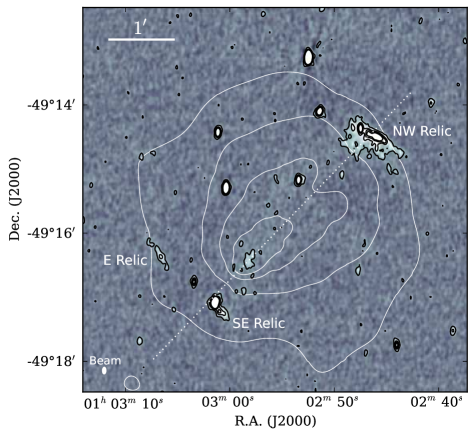
Figure 1.— $2.1\,\rm GHz$ ATCA image of El Gordo. The color stretch is $[-10\sigma,10\sigma]$ and black contours are shown at $3,10,15,20\sigma$, where $\sigma=8.2\,\rm\mu Jy\,beam^{-1}$. White contours represent logarithmic $0.5-2.0\,\rm keV$ X-ray surface brightness (Menanteau et al., 2012). Labels mark the locations of the NW, E, and SE relics. The dotted line represents the estimated collision axis ($\rm P.A.=136^{\circ}$) from Menanteau et al. (2012). The synthesized beam is shown in the lower left corner. The image includes all ATCA data and is produced with multi-frequency synthesis and multi-scale clean.

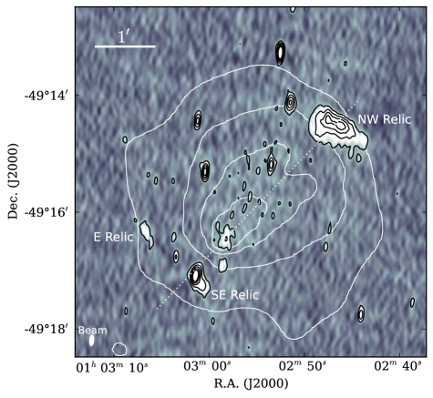
Figure 2.— $610\,\rm MHz$ GMRT image of El Gordo. The color stretch is $[-10\sigma,10\sigma]$ and black contours are shown at $5,15,30,50,75\sigma$, where $\sigma=26\,\rm\mu Jy\,beam^{-1}$. White contours represent logarithmic $0.5-2.0\,\rm keV$ X-ray surface brightness (Menanteau et al., 2012). Labels mark the locations of the NW, E, and SE relics. The dotted line represents the estimated collision axis ($\rm P.A.=136^{\circ}$) from Menanteau et al. (2012). The image includes all GMRT data and is produced with multi-frequency synthesis and multi-scale clean. The synthesized beam is shown in the lower left corner.

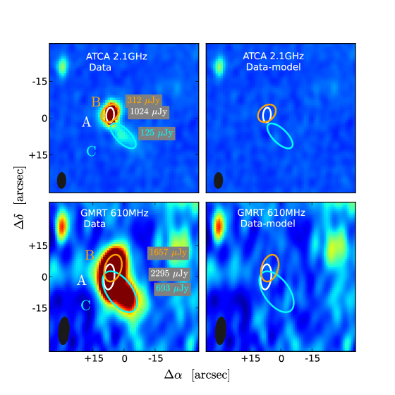
Figure 3.— Gaussian decomposition of the SE relic. The emission is modeled with three elliptical Gaussian components. The contours represent the FWHMs of the best-fit elliptical Gaussians at $2.1\,\rm GHz$ (above) and $610\,\rm MHz$ (below). The original images (left) and model-subtracted residual images (right) are shown. The best-fit peak flux densities for the components are shown in the original image panels. The white, orange, and cyan contours (and text) represent components “A”, “B”, and “C”, respectively (see Section 4.1). The centroids, shape parameters, and numbers of components of the elliptical Gaussian fits were not forced to match between $2.1\,\rm GHz$ and $610\,\rm MHz$; the agreement between frequencies is support for the reality of the SE relic (component C).

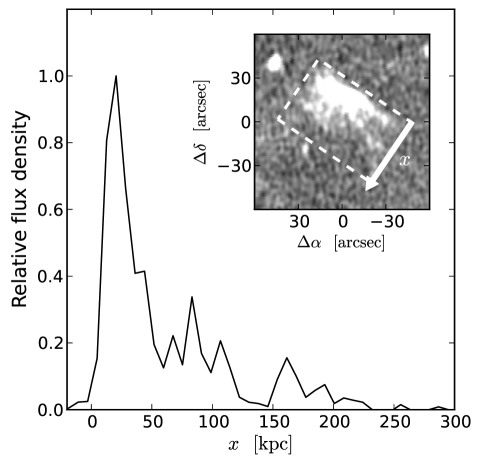
Figure 4.— Projected radial profile of NW relic. The projection region is a $1.3^{\prime}\times 0.8^{\prime}$ box at P.A.=$55^{\circ}$, shown in the inset. The bright leading edge drops quickly, and an extended tail of emission continues out to $\sim 200\,\rm kpc$. The extended tail is due to projection and to the superposition of multiple fainter filaments.

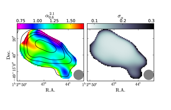
Figure 5.— Spectral index ($\alpha^{2.1}_{0.6}$) map of the NW relic (left) and corresponding uncertainty (right). Contours=[0.3,0.6,1.0,3.0] $\rm mJy\,beam^{-1}$. The filled grey circle represents the effective resolution ($12^{\prime\prime}$).

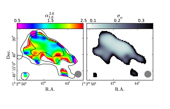
Figure 6.— Spectral index ($\alpha^{2.6}_{1.6}$) map of the NW relic (left) and corresponding uncertainty (right). Contours represent $2.1\,\rm GHz$ intensity levels of 30, 100, and $200\,\rm\mu Jy\,beam^{-1}$. The grey circle represents the effective resolution ($8^{\prime\prime}$).

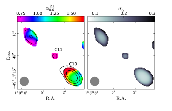
Figure 7.— Spectral index ($\alpha^{2.1}_{0.6}$) map of the E and SE relics (left) and corresponding uncertainty (right). Contours represent $610\,\rm MHz$ intensity levels of $[0.3,0.6,1.0,3.0]\,\rm mJy\,beam^{-1}$. The dotted circle marks the position of subtracted compact source C10. The grey circle represents the effective resolution ($12^{\prime\prime}$).

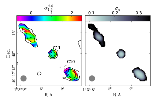
Figure 8.— Spectral index ($\alpha^{2.6}_{1.6}$) map of the E and SE relics (left) and corresponding uncertainty (right). Contours represent $2.1\,\rm GHz$ intensity levels of 30, 100, and $200\,\rm\mu Jy\,beam^{-1}$. The dotted circle marks the position of subtracted compact source C10. The grey circle represents the effective resolution ($8^{\prime\prime}$).

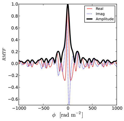
Figure 9.— Rotation measure transfer function of ATCA $2.1\,\rm GHz$ observations. The red and blue lines represent the real and imaginary components; the black line represents the total amplitude.

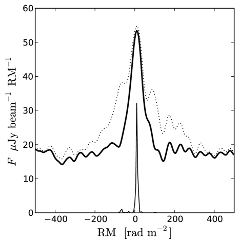
Figure 10.— Integrated RM synthesis spectrum for the NW relic using ATCA ($2.1\,\rm GHz$) data. The dotted and thick solid lines show the uncleaned and cleaned spectra, respectively. The thin solid line below represents the cleaned model components (amplitudes have been scaled by $\times 3$ for visual clarity).

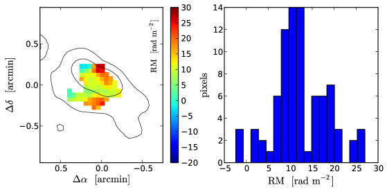
Figure 11.— Left: RM value of dominant RM component in each pixel across the NW relic. RM values are clipped at $>3\sigma$ in the polarized signal image. Stokes $I$ contours are shown at 30 and $300\,\rm\mu Jy\,beam^{-1}$. Right: Distribution of RM values in the left panel. The uncertainty in the RM centroid of a given component ranges between 5–$10\,\rm rad\,m^{-2}$. RM analysis uses ATCA ($2.1\,\rm GHz$) data.

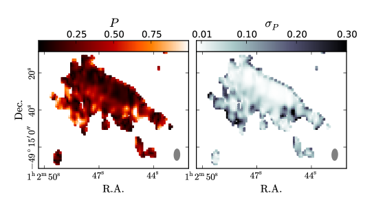
Figure 12.— Polarization fraction $f_{P}$ across the NW relic (left), with corresponding uncertainty (right).

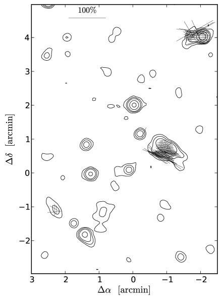
Figure 13.— Polarization fraction $f_{P}$ and angle $\Psi$ of relic emission. Polarization angles have been corrected for rotation measure and further rotated $90^{\circ}$, indicating the direction of $B_{\perp}$. The polarized source in the northwest is SUMSS J010240-491118 with $S_{843}=1.3\,\rm mJy$, and is not associated with the cluster. The $f_{P}=100\%$ scale bar is shown at the top of the panel. The polarization computation is clipped when the Stokes $I$ S/N is $<5\sigma$. Contours of Stokes $I$ emission are drawn at $3,10,25,100,$ and $300\sigma$. The RMS noise in the Stokes $I$ image is $\sigma=12\,\rm\mu Jy\,beam^{-1}$.

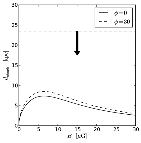
Figure 14.— Predicted shock width as a function of magnetic field strength. The solid and dashed curves show predictions of $d_{\rm shock}$ using projection angles $\phi=0$ and $30^{\circ}$, respectively. The horizontal dashed line and downward arrow represent the upper limit placed on the shock width from our $2.1\,\rm GHz$ imaging ($d_{\rm shock}\leq 23\,\rm kpc$).

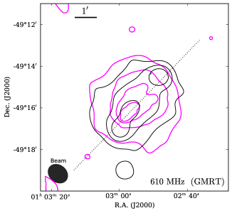
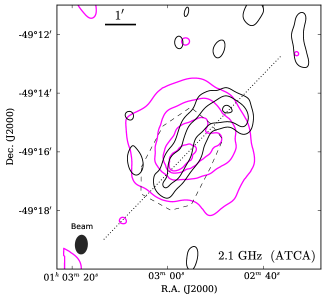
Figure 15.— El Gordo’s $610\,\rm MHz$ (left) and $2.1\,\rm GHz$ (right) radio halo. Black contours represent the surface brightess S/N with levels at $3,10,20,40,70\sigma$ where $\sigma_{610}=155\,\rm\mu Jy\,beam^{-1}$ and $\sigma_{2.1}=28.4\,\rm\mu Jy\,beam^{-1}$. Purple contours represent logarithmic $0.5-2.0\,\rm keV$ X-ray surface brightness (Menanteau et al., 2012). The synthesized beam shapes are shown in the lower left-hand corners of the panels. To maximize sensitivity to the diffuse, low surface-brightness halo emission, the halo images are produced with $uv$ data that have had compact emission from point sources and relics (i.e., most structures visible in Figures 1 and 2) subtracted out, and with reduced spatial resolution. The dashed polygon represents the region used to compute the halo’s integrated spectral index and excludes the area near the NW relic.

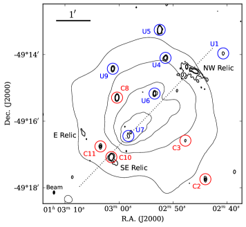
Figure 16.— Locations of compact radio sources with $\rm S/N>5$ in the El Gordo field. Sources are labeled with prefix ‘C’ and circled in red if they are spectroscopically-confirmed cluster members (Sifón et al., 2013), or labeled with prefix ’U’ and circled in blue if they are unrelated to the cluster. Table THE RADIO RELICS AND HALO OF EL GORDO, A MASSIVE $z=0.870$ CLUSTER MERGER lists the sources’ positions and flux densities.

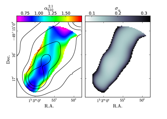
Figure 17.— Spectral index $\alpha^{2.1}_{0.6}$ image of El Gordo’s radio halo. The spectral index and the uncertainty per pixel $\sigma_{\alpha}$ are shown in the left and right panels, respectively. Contours represent the $610\,\rm MHz$ halo intensity with levels 1, 2, 3, and $4\,\rm mJy\,beam^{-1}$.

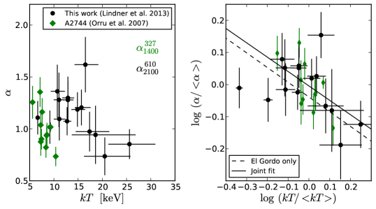
Figure 18.— Left: Spatially resolved measurements of radio spectral index versus X-ray gas temperature for El Gordo (black points) compared to A2744 (Orrú et al., 2007). Right: Linear fits to the $\log$ of the data in the left panel after scaling by the means ($\left<kT\right>_{\rm A2744}=8.0\,\rm keV$, $\left<kT\right>_{\rm El\;Gordo}=14.6\,\rm keV$). The dashed line shows the best-fit when we use El Gordo data only (power-law slope $B\simeq-0.5$), and the solid line shows the best fit when we use both datasets together ($B\simeq-0.4$).

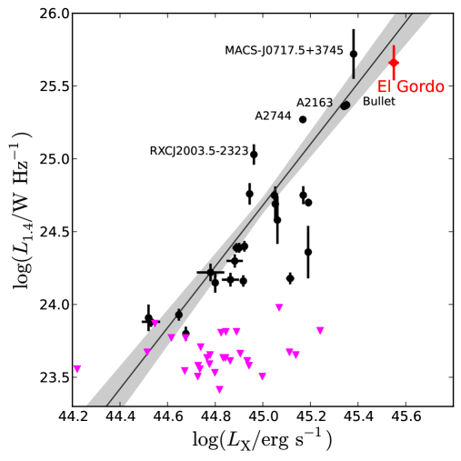
Figure 19.— Rest-frame $20\,\rm cm$ spectral power vs. $L_{X}$ for El Gordo’s and other halos from the literature tabulated in Cassano et al. (2013). Labels are provided for halos with $\log(L_{1.4}/\rm W\,Hz^{-1})>25$. The purple triangles represent upper limits. Errors in $\log L_{1.4}$ for El Gordo’s halo include the uncertainty in $\alpha^{2.1}_{0.6}$ used in the k-correction. The line and shaded region show the fit best correlation and $\pm 1\sigma$ uncertainties from Cassano et al. (2013).

Table 1Radio observations

				$t_{\rm obs}$	$B_{\rm min}$–$B_{\rm max}$
Telescope	Frequency	Configuration	Obs date	(hr)	($\rm k\lambda$)
ATCA	$2.1\,\rm GHz$	6A	Dec 2011	12	2.4–41.6
		1.5B	April 2012	8	1.4–30.1
GMRT	$610\,\rm MHz$	fixed	Aug 2012	12	0.48–52.8

Table 2Radio sources

	R.A.	Dec.	$S_{610}\tablenotemark{b}$	$S_{2100}\tablenotemark{b}$
ID	(h:m:s)	($\circ:\prime:\prime\prime$)	($\mu$Jy)	($\mu$Jy)
U1	01:02:40.74	-49:13:58.09	-	$104\pm 15$
C2	01:02:44.02	-49:17:44.90	$614\pm 77$	$253\pm 19$
C3	01:02:47.72	-49:16:35.41	$235\pm 53$	$87\pm 17$
U4	01:02:51.40	-49:14:06.21	$1953\pm 205$	$606\pm 34$
U5	01:02:52.47	-49:13:15.71	$5085\pm 511$	$5044\pm 253$
U6	01:02:53.42	-49:15:10.50	$1021\pm 112$	$503\pm 29$
U7	01:02:58.26	-49:16:27.01	$590\pm 96$	-
C8	01:03:00.35	-49:15:17.83	$1761\pm 182$	$1612\pm 82$
U9	01:03:01.13	-49:14:25.79	$1068\pm 118$	$549\pm 31$
C10	01:03:01.41	-49:17:05.11	$5750\pm 579$	$1859\pm 94$
C11	01:03:03.43	-49:16:45.73	$331\pm 50$

Table 3Relic and halo properties

References

- Baars et al. (1977) Baars, J. W. M., Genzel, R., Pauliny-Toth, I. I. K., & Witzel, A. 1977, A&A, 61, 99
- Bonafede et al. (2013) Bonafede, A., Vazza, F., Brüggen, M., et al. 2013, MNRAS, 433, 3208
- Bonafede et al. (2009) Bonafede, A., Feretti, L., Giovannini, G., et al. 2009, A&A, 503, 707
- Bonafede et al. (2012) Bonafede, A., Brüggen, M., van Weeren, R., et al. 2012, MNRAS, 426, 40
- Boschin et al. (2006) Boschin, W., Girardi, M., Spolaor, M., & Barrena, R. 2006, A&A, 449, 461
- Brentjens & de Bruyn (2005) Brentjens, M. A., & de Bruyn, A. G. 2005, A&A, 441, 1217
- Brown et al. (2011) Brown, S., Duesterhoeft, J., & Rudnick, L. 2011, ApJ, 727, L25
- Brunetti et al. (2009) Brunetti, G., Cassano, R., Dolag, K., & Setti, G. 2009, A&A, 507, 661
- Brunetti et al. (2001) Brunetti, G., Setti, G., Feretti, L., & Giovannini, G. 2001, MNRAS, 320, 365
- Buote (2001) Buote, D. A. 2001, ApJ, 553, L15
- Burn (1966) Burn, B. J. 1966, MNRAS, 133, 67
- Carlstrom et al. (2011) Carlstrom, J. E., Ade, P. A. R., Aird, K. A., et al. 2011, PASP, 123, 568
- Cassano et al. (2007) Cassano, R., Brunetti, G., Setti, G., Govoni, F., & Dolag, K. 2007, MNRAS, 378, 1565
- Cassano et al. (2011) Cassano, R., Brunetti, G., & Venturi, T. 2011, Journal of Astrophysics and Astronomy, 32, 519
- Cassano et al. (2013) Cassano, R., Ettori, S., Brunetti, G., et al. 2013, ApJ, 777, 141
- Chandra et al. (2004) Chandra, P., Ray, A., & Bhatnagar, S. 2004, ApJ, 604, L97
- Cornwell (2008) Cornwell, T. J. 2008, IEEE Journal of Selected Topics in Signal Processing, 2, 793
- Dennison (1980) Dennison, B. 1980, ApJ, 239, L93
- Drury (1983) Drury, L. O. 1983, Reports on Progress in Physics, 46, 973
- Ensslin et al. (1998) Ensslin, T. A., Biermann, P. L., Klein, U., & Kohle, S. 1998, A&A, 332, 395
- Feretti et al. (2012) Feretti, L., Giovannini, G., Govoni, F., & Murgia, M. 2012, A&A Rev., 20, 54
- Feretti et al. (2004) Feretti, L., Orrù, E., Brunetti, G., et al. 2004, A&A, 423, 111
- Feretti et al. (2005) Feretti, L., Schuecker, P., Böhringer, H., Govoni, F., & Giovannini, G. 2005, A&A, 444, 157
- Ferrari et al. (2008) Ferrari, C., Govoni, F., Schindler, S., Bykov, A. M., & Rephaeli, Y. 2008, Space Sci. Rev., 134, 93
- Fowler et al. (2007) Fowler, J. W., Niemack, M. D., Dicker, S. R., et al. 2007, Appl. Opt., 46, 3444
- Giacintucci et al. (2013) Giacintucci, S., Kale, R., Wik, D. R., Venturi, T., & Markevitch, M. 2013, ApJ, 766, 18
- Girardi et al. (2008) Girardi, M., Barrena, R., Boschin, W., & Ellingson, E. 2008, A&A, 491, 379
- Govoni & Feretti (2004) Govoni, F., & Feretti, L. 2004, International Journal of Modern Physics D, 13, 1549
- Hinshaw et al. (2013) Hinshaw, G., Larson, D., Komatsu, E., et al. 2013, ApJS, 208, 19
- Jee et al. (2013) Jee, M. J., Hughes, J. P., Menanteau, F., et al. 2013, ArXiv e-prints, arXiv:1309.5097
- Markevitch et al. (2002) Markevitch, M., Gonzalez, A. H., David, L., et al. 2002, ApJ, 567, L27
- Marriage et al. (2011) Marriage, T. A., Acquaviva, V., Ade, P. A. R., et al. 2011, ApJ, 737, 61
- Mauch et al. (2003) Mauch, T., Murphy, T., Buttery, H. J., et al. 2003, MNRAS, 342, 1117
- Menanteau et al. (2010) Menanteau, F., González, J., Juin, J.-B., et al. 2010, ApJ, 723, 1523
- Menanteau et al. (2012) Menanteau, F., Hughes, J. P., Sifón, C., et al. 2012, ApJ, 748, 7
- Middelberg (2006) Middelberg, E. 2006, PASA, 23, 64
- Nagai et al. (2007) Nagai, D., Kravtsov, A. V., & Vikhlinin, A. 2007, ApJ, 668, 1
- Nuza et al. (2012) Nuza, S. E., Hoeft, M., van Weeren, R. J., Gottlöber, S., & Yepes, G. 2012, MNRAS, 420, 2006
- Offringa et al. (2010) Offringa, A. R., de Bruyn, A. G., Biehl, M., et al. 2010, MNRAS, 405, 155
- Offringa et al. (2012) Offringa, A. R., van de Gronde, J. J., & Roerdink, J. B. T. M. 2012, A&A, 539, A95
- Oppermann et al. (2012) Oppermann, N., Junklewitz, H., Robbers, G., et al. 2012, A&A, 542, A93
- Orrú et al. (2007) Orrú, E., Murgia, M., Feretti, L., et al. 2007, A&A, 467, 943
- O’Sullivan et al. (2012) O’Sullivan, S. P., Brown, S., Robishaw, T., et al. 2012, MNRAS, 421, 3300
- Pfrommer et al. (2008) Pfrommer, C., Enßlin, T. A., & Springel, V. 2008, MNRAS, 385, 1211
- Reynolds (1994) Reynolds, J. E. 1994, ATNF Technical Document Series, AT/39.3/0400
- Rybicki & Lightman (1979) Rybicki, G. B., & Lightman, A. P. 1979, Radiative processes in astrophysics (New York, Wiley-Interscience, 1979)
- Sault et al. (1995) Sault, R. J., Teuben, P. J., & Wright, M. C. H. 1995, in Astronomical Society of the Pacific Conference Series, Vol. 77, Astronomical Data Analysis Software and Systems IV, ed. R. A. Shaw, H. E. Payne, & J. J. E. Hayes, 433
- Schnitzeler et al. (2011) Schnitzeler, D., Banfield, J., Emonts, B., et al. 2011, ATNF Technical Document Series, AT/39.9/129
- Sifón et al. (2013) Sifón, C., Menanteau, F., Hasselfield, M., et al. 2013, ApJ, 772, 25
- Sommer & Basu (2014) Sommer, M. W., & Basu, K. 2014, MNRAS, 437, 2163
- Sunyaev & Zeldovich (1972) Sunyaev, R. A., & Zeldovich, Y. B. 1972, Comments on Astrophysics and Space Physics, 4, 173
- Vacca et al. (2014) Vacca, V., Feretti, L., Giovannini, G., et al. 2014, A&A, 561, A52
- van Weeren et al. (2012) van Weeren, R. J., Bonafede, A., Ebeling, H., et al. 2012, MNRAS, 425, L36
- van Weeren et al. (2011a) van Weeren, R. J., Brüggen, M., Röttgering, H. J. A., & Hoeft, M. 2011a, MNRAS, 418, 230
- van Weeren et al. (2011b) van Weeren, R. J., Hoeft, M., Röttgering, H. J. A., et al. 2011b, A&A, 528, A38
- van Weeren et al. (2009a) van Weeren, R. J., Röttgering, H. J. A., Brüggen, M., & Cohen, A. 2009a, A&A, 505, 991
- van Weeren et al. (2010) van Weeren, R. J., Röttgering, H. J. A., Brüggen, M., & Hoeft, M. 2010, Science, 330, 347
- van Weeren et al. (2009b) van Weeren, R. J., Röttgering, H. J. A., Bagchi, J., et al. 2009b, A&A, 506, 1083
- van Weeren et al. (2014) van Weeren, R. J., Intema, H. T., Lal, D. V., et al. 2014, ApJ, 781, L32
- Venturi et al. (2007) Venturi, T., Giacintucci, S., Brunetti, G., et al. 2007, A&A, 463, 937
- Venturi et al. (2008) Venturi, T., Giacintucci, S., Dallacasa, D., et al. 2008, A&A, 484, 327
- Wardle & Kronberg (1974) Wardle, J. F. C., & Kronberg, P. P. 1974, ApJ, 194, 249
- Williamson et al. (2011) Williamson, R., Benson, B. A., High, F. W., et al. 2011, ApJ, 738, 139
- Wilson et al. (2011) Wilson, W. E., Ferris, R. H., Axtens, P., et al. 2011, MNRAS, 416, 832
- Zitrin et al. (2013) Zitrin, A., Menanteau, F., Hughes, J. P., et al. 2013, ApJ, 770, L15