Romantic Partnerships and the Dispersion of Social Ties:
A Network Analysis of Relationship Status on Facebook

Abstract

A crucial task in the analysis of on-line social-networking systems is to identify important people — those linked by strong social ties — within an individual’s network neighborhood. Here we investigate this question for a particular category of strong ties, those involving spouses or romantic partners. We organize our analysis around a basic question: given all the connections among a person’s friends, can you recognize his or her romantic partner from the network structure alone? Using data from a large sample of Facebook users, we find that this task can be accomplished with high accuracy, but doing so requires the development of a new measure of tie strength that we term ‘dispersion’ — the extent to which two people’s mutual friends are not themselves well-connected. The results offer methods for identifying types of structurally significant people in on-line applications, and suggest a potential expansion of existing theories of tie strength.

Categories and Subject Descriptors: H.2.8 [Database Management]: Database applications—Data mining

Keywords: Social Networks; Romantic Relationships.

1 Introduction

In a social network, an individual’s network neighborhood — the set of people to whom he or she is linked — has been shown to have important consequences in a wide range of settings, including social support [12, 24] and professional opportunities [15, 5]. As people use on-line social networks to manage increasingly rich aspects of their lives, the structures of their on-line network neighborhoods have come to reflect these functions, and the complexity that goes with them.

A person’s network neighbors, taken as a whole, encompass a profoundly diverse set of relationships — they typically include family members, co-workers, friends of long duration, distant acquaintances, potentially a spouse or romantic partner, and a variety of other categories. An important and very broad issue for the analysis of on-line social networks is to use features in the available data to recognize this variation across types of relationships. Methods to do this effectively can play an important role for many applications at the interface between an individual and the rest of the network — managing their on-line interactions [9], prioritizing content they see from friends [1], and organizing their neighborhood into conceptually coherent groups [23, 25].

Tie Strength.

Tie strength forms an important dimension along which to characterize a person’s links to their network neighbors. Tie strength informally refers to the ‘closeness’ of a friendship; it captures a spectrum that ranges from strong ties with close friends to weak ties with more distant acquaintances. An active line of research reaching back to foundational work in sociology has studied the relationship between the strengths of ties and their structural role in the underlying social network [15]. Strong ties are typically ‘embedded’ in the network, surrounded by a large number of mutual friends [16, 6], and often involving large amounts of shared time together [22] and extensive interaction [17]. Weak ties, in contrast, often involve few mutual friends and can serve as ‘bridges’ to diverse parts of the network, providing access to novel information [15, 5].

A fundamental question connected to our understanding of strong ties is to identify the most important individuals in a person’s social network neighborhood using the underlying network structure. What are the defining structural signatures of a person’s strongest ties, and how do we recognize them? Techniques for this problem have potential importance both for organizing a person’s network neighborhood in on-line applications, and also for providing basic insights into the effect of close relationships on network structure more broadly.

Recent work has developed methods of analyzing and estimating tie strength in on-line domains, drawing on data from e-mail [19], phone calls [27], and social media [14]. The key structural feature used in these analyses is the notion of embeddedness — the number of mutual friends two people share [22], a quantity that typically increases with tie strength. Indeed, embeddedness has been so tightly associated with tie strength that it has remained largely an open question to determine whether there are other structural measures, distinct from embeddedness, that may be more appropriate for characterizing particular types of strong ties.

Romantic Relationships.

In this work we propose a new network-based characterization for intimate relationships, those involving spouses or romantic partners. Such relationships are important to study for several reasons.

From a substantive point of view, romantic relationships are of course singular types of social ties that play powerful roles in social processes over a person’s whole life course [4], from adolescence [2] to older age [7]. They also form an important aspect of the everyday practices and uses of social media [28]. And they are an important challenge from a methodological point of view; they are evidently among the very strongest ties, but it has not been clear whether standard structural theories based on embeddedness are sufficient to characterize them, or whether they possess singular structural properties of their own [11, 18].

Our central finding is that embeddedness is in fact a comparatively weak means of characterizing romantic relationships, and that an alternate network measure that we term dispersion is significantly more effective. Our measure of dispersion looks not just at the number of mutual friends of two people, but also at the network structure on these mutual friends; roughly, a link between two people has high dispersion when their mutual friends are not well connected to one another.

On a large random sample of Facebook users who have declared a relationship partner in their profile, we find that our dispersion measure has roughly twice the accuracy of embeddedness in identifying this partner from among the user’s full set of friends. Indeed, for married Facebook users, our measure of dispersion applied to the pure, unannotated network structure is more effective at identifying a user’s spouse than a complex classifier trained using machine learning on an array of interaction measures including messaging, commenting, profile-viewing, and co-presence at events and in photos. Further, using dispersion in conjunction with these interaction features produces significantly higher accuracy.

The main contributions of our work are thus the following.

• We propose a new network measure, dispersion, for estimating tie strength. Given the ubiquity of embeddedness in existing analyses of tie strength, the availability of this new measure broadens the range of tools available for reasoning about tie strength, and about mechanisms for tie-strength classification in on-line domains.

• We provide a new substantive characterization of romantic relationships in terms of network structure, with potential consequences for our understanding of the effect that such relationships have on the underlying social network.

• Given this characterization, we examine its variation across different conditions and populations. We find, for example, that there are significant gender differences in the extent to which relationship partners are recognizable from network structure, and that relationships are more likely to persist when they score highly under our dispersion measure.

It is also important to delineate the scope of our results. Our approach to analyzing romantic partnerships in on-line social settings is through their effect on the network structure, and the ways in which such relationships can be recognized through their structural signatures. As such, there is potential for it to be combined with other perspectives on how these relationships are expressed on-line, and the conventions that develop around their on-line expression; a complete picture will necessarily involve a synthesis of all these perspectives.

2 Data and Problem Description

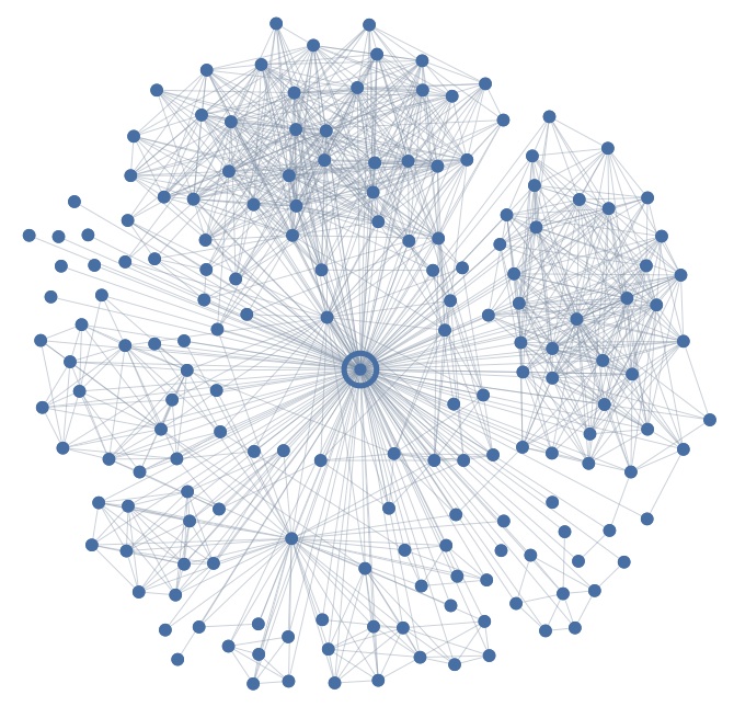
We analyze romantic relationships in social networks using a dataset of randomly sampled Facebook users who declared a relationship partner in their profile; this includes users who listed their status as ‘married,’ ‘engaged,’ or ‘in a relationship’. To evaluate different structural theories on a common footing, we begin with a simply stated prediction task designed to capture the basic issues. We take a Facebook user with a declared relationship partner, and we hide the identity of this partner. Then we ask: given the user’s network neighborhood — the set of all friends and the links among them — how accurately can we identify the relationship partner using this structural information alone? Figure 1 gives an example of such a Facebook user’s network neighborhood[21], drawn so that the user is depicted at the center; such diagrams are the ‘input’ from which we wish to identify the user’s partner. By phrasing the question this starkly, we are able to assess the extent to which structural information on its own conveys information about the relationships of interest.

We note that our question has an important contingent nature: given that a user has declared a relationship partner, we want to understand how effectively we can find the partner. There are different questions that could be asked in a related vein — for example, inferring from a user’s network neighborhood whether he or she is in a relationship. We briefly discuss the connections among these questions in a subsequent section, but the problem of identifying partners is our main focus here.

As data for our analyses, we principally use two collections of network neighborhoods from Facebook. The first consists of the network neighborhoods of approximately 1.3 million Facebook users, selected uniformly at random from among all users of age at least 20, with between 50 and 2000 friends, who list a spouse or relationship partner in their profile. These neighborhoods have an average of 291 nodes and 6652 links, for an overall dataset containing roughly 379 million nodes and 8.6 billion links.

We also employ a smaller dataset — a sample of approximately 73000 neighborhoods from this first collection, selected uniformly at random from among all neighborhoods with at most 25000 links. We refer to this sample as the primary dataset, and the larger dataset in the preceding paragraph as the extended dataset. We compute our main structural and interaction measures on both the primary and extended datasets, and these measures exhibit nearly identical performance on the two datasets. As we discuss further below, we evaluate additional network measures, as well as more complex combinations of measures based on machine learning algorithms, only on the primary dataset.

All Facebook data in these analyses was used anonymously, and all analysis was done in aggregate.

3 Embeddedness and Dispersion

To evaluate approaches for our task of recognizing relationship partners from network structure, we start with a fundamental baseline — the standard characterization of a tie’s strength in terms of its embeddedness, the number of mutual friends shared by its endpoints [22]. Embeddedness has also served as the key definition in structural analyses for the special case of relationship partners, since it captures how much the two partners’ social circles ‘overlap’ [11, 18]. This suggests a natural predictor for identifying a user $u$’s partner: select the link from $u$ of maximum embeddedness, and propose the other end $v$ of this link as $u$’s partner.

We will evaluate this embeddedness-based predictor, and others, according to their performance: the fraction of instances on which they correctly identify the partner. Under this measure, embeddedness achieves a performance of $24.7\%$ — which both provides evidence about the power of structural information for this task, but also offers a baseline that other approaches can potentially exceed.

Next, we show that it is possible to achieve more than twice the performance of this embeddedness baseline using our new network measure, dispersion. In addition to this relative improvement, the performance of our dispersion measure is very high in an absolute sense — for example, on married users in our sample, the friend who scores highest under this dispersion measure is the user’s spouse over 60% of the time. Since each user in our sample has at least 50 friends, this performance is more than 30 times higher than random guessing, which would produce a performance of at most 2%.

Figure 1: A network neighborhood, contributed by a Facebook employee (drawn as the circled node at the center), and displayed as an example in the work of Marlow et al[21]. Two clear clusters with highly embedded links are visible at the top and right of the diagram; in the lower left of the diagram are smaller, sparser clusters together with a node that bridges between these clusters.

Figure 2: A synthetic example network neighborhood for a user $u$; the links from $u$ to $b$, $c$, and $f$ all have embeddedness 5 (the highest value in this neighborhood), whereas the link from $u$ to $h$ has an embeddedness of 4. On the other hand, nodes $u$ and $h$ are the unique pair of intermediaries from the nodes $c$ and $f$ to the nodes $j$ and $k$; the $u$-$h$ link has greater dispersion than the links from $u$ to $b$, $c$, and $f$.

Theoretical Basis for Dispersion.

We motivate the dispersion measure by first highlighting a basic limitation of embeddedness as a predictor, drawing on the theory of social foci [10]. Many individuals have large clusters of friends corresponding to well-defined foci of interaction in their lives, such as their cluster of co-workers or the cluster of people with whom they attended college. Since many people within these clusters know each other, the clusters contain links of very high embeddedness, even though they do not necessarily correspond to particularly strong ties. In contrast, the links to a person’s relationship partner or other closest friends may have lower embeddedness, but they will often involve mutual neighbors from several different foci, reflecting the fact that the social orbits of these close friends are not bounded within any one focus — consider, for example, a husband who knows several of his wife’s co-workers, family members, and former classmates, even though these people belong to different foci and do not know each other.

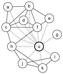
Thus, instead of embeddedness, we propose that the link between an individual $u$ and his or her partner $v$ should display a ‘dispersed’ structure: the mutual neighbors of $u$ and $v$ are not well-connected to one another, and hence $u$ and $v$ act jointly as the only intermediaries between these different parts of the network. (See Figure 2 for an illustration.)

We now formulate a sequence of definitions that captures this idea of dispersion. To begin, we take the subgraph $G_{u}$ induced on $u$ and all neighbors of $u$, and for a node $v$ in $G_{u}$ we define $C_{uv}$ to be the set of common neighbors of $u$ and $v$. To express the idea that pairs of nodes in $C_{uv}$ should be far apart in $G_{u}$ when we do not consider the two-step paths through $u$ and $v$ themselves, we define the absolute dispersion of the $u$-$v$ link, $disp(u,v)$, to be the sum of all pairwise distances between nodes in $C_{uv}$, as measured in $G_{u}-\{u,v\}$; that is,

$$disp(u,v)=\sum_{s,t\in C_{uv}}d_{v}(s,t),$$

where $d_{v}$ is a distance function on the nodes of $C_{uv}$. The function $d_{v}$ need not be the standard graph-theoretic distance; different choices of $d_{v}$ will give rise to different measures of absolute dispersion. As we discuss in more detail below, among a large class of possible distance functions, we ultimately find the best performance when we define $d_{v}(s,t)$ to be the function equal to $1$ when $s$ and $t$ are not directly linked and also have no common neighbors in $G_{u}$ other than $u$ and $v$, and equal to $0$ otherwise. For the present discussion, we will use this distance function as the basis for our measures of dispersion; below we consider the effect of alternative distance functions. For example, in Figure 2, $disp(u,h)=4$ under this definition and distance function, since there are four pairs of nodes in $C_{uh}$ that are not directly linked and also have no neighbors in common in $G_{u}-\{u,h\}$. In contrast, $disp(u,b)=1$ in Figure 2, since $a$ and $e$ form the only pair of non-neighboring nodes in $C_{ub}$ that have no neighbors in common in $G_{u}-\{u,b\}$.

Figure 3: Performance of $(disp(u,v)+b)^{\alpha}/(emb(u,v)+c)$ as a function of $\alpha$, when choosing optimal values of $b$ and $c$.

type	embed	rec.disp.	photo	prof.view.
all	0.247	0.506	0.415	0.301
married	0.321	0.607	0.449	0.210
married (fem)	0.296	0.551	0.391	0.202
married (male)	0.347	0.667	0.511	0.220
engaged	0.179	0.446	0.442	0.391
engaged (fem)	0.171	0.399	0.386	0.401
engaged (male)	0.185	0.490	0.495	0.381
relationship	0.132	0.344	0.347	0.441
relationship (fem)	0.139	0.316	0.290	0.467
relationship (male)	0.125	0.369	0.399	0.418

Figure 4: The performance of different measures for identifying spouses and romantic partners: the numbers in the table give the precision at the first position — the fraction of instances in which the user ranked first by the measure is in fact the true partner. Averaged over all instances, recursive dispersion performs approximately twice as well as the standard notion of embeddedness, and also better overall than measures based on profile viewing and presence in the same photo.

type	embed	rec.disp.	photo	prof.view.
all	0.391	0.688	0.528	0.389
married	0.462	0.758	0.561	0.319
married (fem)	0.488	0.764	0.538	0.350
married (male)	0.435	0.751	0.586	0.287
engaged	0.335	0.652	0.553	0.457
engaged (fem)	0.375	0.674	0.536	0.492
engaged (male)	0.296	0.630	0.568	0.424
relationship	0.277	0.572	0.460	0.498
relationship (fem)	0.318	0.600	0.440	0.545
relationship (male)	0.239	0.546	0.479	0.455

Figure 5: The performance of the four measures from Figure 4 when the goal is to identify the partner or a family member in the first position of the ranked list. The difference in performance between the genders has largely vanished, and in some cases is inverted relative to Figure 4.

Strengthenings of Dispersion.

We can learn a function that predicts whether or not $v$ is the partner of $u$ in terms of the two variables $disp(u,v)$ and $emb(u,v)$, where the latter denotes the embeddedness of the $u$-$v$ link. We find that performance is highest for functions that are monotonically increasing in $disp(u,v)$ and monotonically decreasing in $emb(u,v)$: for a fixed value of $disp(u,v)$, increased embeddedness is in fact a negative predictor of whether $v$ is the partner of $u$. A simple combination of these two quantities that comes within a few percent of more complicated functional forms can be obtained by the expression $disp(u,v)/emb(u,v)$, which we term the normalized dispersion $norm(u,v)$ since it normalizes the absolute dispersion by the embeddedness. Predicting $u$’s partner to be the individual $v$ maximizing $norm(u,v)$ gives the correct answer in $48.0\%$ of all instances.

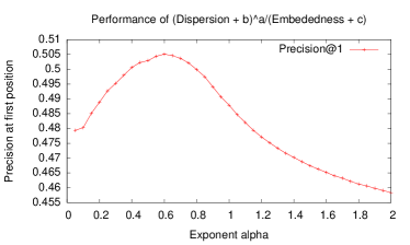
There are two strengthenings of the normalized dispersion that lead to increased performance. The first is to rank nodes by a function of the form $(disp(u,v)+b)^{\alpha}/(emb(u,v)+c)$. Searching over choices of $\alpha$, $b$, and $c$ leads to maximum performance of $50.5\%$ at $\alpha=0.61$, $b=0$, and $c=5$; see Figure 3. Alternately, one can strengthen performance by applying the idea of dispersion recursively — identifying nodes $v$ for which the $u$-$v$ link achieves a high normalized dispersion based on a set of common neighbors $C_{uv}$ who, in turn, also have high normalized dispersion in their links with $u$. To carry out this recursive idea, we assign values to the nodes reflecting the dispersion of their links with $u$, and then update these values in terms of the dispersion values associated with other nodes. Specifically, we initially define $x_{v}=1$ for all neighbors $v$ of $u$, and then iteratively update each $x_{v}$ to be

$$\frac{\sum_{w\in C_{uv}}x_{w}^{2}+2\sum_{s,t\in C_{uv}}d_{v}(s,t)x_{s}x_{t}}{emb(u,v)}.$$

Note that after the first iteration, $x_{v}$ is $1+2\cdot norm(u,v)$, and hence ranking nodes by $x_{v}$ after the first iteration is equivalent to ranking nodes by $norm(u,v)$. We find the highest performance when we rank nodes by the values of $x_{v}$ after the third iteration. For purposes of later discussion, we will call this value $x_{v}$ in the third iteration the recursive dispersion $rec(u,v)$, and will focus on this as the main examplar from our family of related dispersion-based measures. (See the Appendix for further mathematical properties of the recursive dispersion.)

4 Performance of Structural and Interaction Measures

We summarize the performance of our methods in Figure 4. Looking initially at just the first two columns in the top row of numbers (‘all’), we have the overall performance of embeddedness and recursive dispersion — the fraction of instances on which the highest-ranked node under these measures is in fact the partner. As we will see below in the discussion around Figure 6, recursive dispersion also has higher performance than a wide range of other basic structural measures.

We can also compare these structural measures to features derived from a variety of different forms of real-time interaction between users — including the viewing of profiles, sending of messages, and co-presence at events. The use of such ‘interaction features’ as a comparison baseline is motivated by the way in which tie strength can be estimated from the volume of interaction between two people [8, 17]. Within this category of interaction features, the two that consistently display the best performance are to rank neighbors of $u$ by the number of photos in which they appear with $u$, and to rank neighbors of $u$ by the total number of times that $u$ has viewed their profile page in the previous 90 days. The last two columns of Figure 4 show the performance of these two measures; on the set of instances as a whole, recursive dispersion performs better than these features.

The remaining rows of Figure 4 show the performance of these measures on different subsets of the data. Most users who report a relationship partner on Facebook list themselves as either ‘married’ or ‘in a relationship,’ with a smaller number who are ‘engaged.’ The performance of the structural measures is much higher for married users (60.7%) than for users in a relationship (34.4%); the opposite is true for profile viewing, which in fact achieves higher performance than recursive dispersion for users in a relationship. The performance for users who are engaged is positioned between the extremes of ‘married’ and ‘in a relationship.’

In addition, we see important differences based on gender. The performance of structural measures is significantly higher for males than for females, suggesting some of the ways in which relationship partners produce more visible structural effects — at least according to these measures — on the network neighborhoods of men. And for certain more focused subsets of the data, the performance is even stronger; for example, on the subset corresponding to married male Facebook users in the United States, the friend with the highest recursive dispersion is the user’s spouse $76.9\%$ of the time.

We can also evaluate performance on the subset of users in same-sex relationships. Here we focus on users whose status is ‘in a relationship.’ The relative performance of our structural measures is exactly the same for same-sex relationships as for the set of all relationships, with recursive dispersion achieving close to twice the performance of embeddedness, and slightly higher performance than absolute and normalized dispersion. For female users, the absolute level of performance is almost identical regardless of whether their listed partner is female or male; for male users, the performance is significantly higher for relationships in which the partner is male. (For a same-sex relationship listed by a male user, recursive dispersion identifies the partner with a performance of $.450$, in contrast with the performance of $.369$ for all partners of male users shown in Figure 4.)

Finally, returning to the set of all relationships, when the user $v$ who scores highest under one of these measures is not the partner of $u$, what role does $v$ play among $u$’s network neighbors? We find that $v$ is often a family member of $u$; for married users (Figure 5), the friend $v$ that maximizes $rec(u,v)$ is the partner or a family member over $75\%$ of the time. We also see that when we ask for the top-ranked friend to be either the partner or a family member, rather than just the partner, the performance gap between the genders essentially vanishes in the case of married users, and becomes inverted in the case of users in a relationship — in this latter case, female users are more likely to have their partner or a family member at the top of the ranking by recursive dispersion.

distance	type	all	marr.	eng.	rel.
threshold 2	absolute	0.279	0.361	0.205	0.152
	normalized	0.305	0.394	0.227	0.168
	recursive	0.210	0.279	0.141	0.105
threshold 3	absolute	0.430	0.530	0.359	0.270
	normalized	0.486	0.588	0.425	0.322
	recursive	0.506	0.607	0.446	0.344
threshold 4	absolute	0.473	0.568	0.414	0.321
	normalized	0.483	0.570	0.434	0.342
	recursive	0.455	0.539	0.405	0.319
diff component	absolute	0.380	0.461	0.317	0.253
	normalized	0.364	0.433	0.308	0.258
	recursive	0.323	0.384	0.276	0.228
diff community	absolute	0.286	0.368	0.212	0.160
	normalized	0.296	0.379	0.221	0.167
	recursive	0.216	0.283	0.156	0.115
spring length	absolute	0.379	0.474	0.307	0.229
	normalized	0.454	0.553	0.387	0.296
	recursive	0.396	0.480	0.341	0.261

Figure 6: Performance of variants of the dispersion measure using different underlying distance functions.

measure	all	married	engaged	relationship
betweenness	0.441	0.535	0.374	0.293
network constraint	0.307	0.394	0.232	0.171

Figure 7: Performance of betweenness and network constraint as alternate measures of bridging.

A Broader Set of Measures.

Since measures of dispersion are based on an underlying distance function $d_{v}$, it is interesting to investigate how the performance depends on the choice of $d_{v}$. In Figure 6, we consider dispersion measures based on a range of natural choices for $d_{v}$. as follows.

• First, we can set a distance threshold $r$, and declare that $d_{v}(s,t)=1$ when $s$ and $t$ are at least $r$ hops apart in $G_{u}-\{u,v\}$, and $d_{v}(s,t)=0$ otherwise. The measure of dispersion we use above corresponds to the choice $r=3$; setting the threshold $r=2$ simply requires that $s$ and $t$ are not directly connected, while setting $r=4$ imposes a stricter requirement.

• In a related vein, we could declare $d_{v}(s,t)=1$ if $s$ and $t$ belong to different connected components of $G_{u}-\{u,v\}$, and $d_{v}(s,t)=0$ otherwise. This in effect follows the preceding approach, but with the distance threshold $r$ conceptually set to be infinite.

• Since the idea of dispersion at a more general level is based on the notion that the common neighbors of $u$ and $v$ should belong to different ‘parts’ of the network, it is also natural to divide $G_{u}-\{u\}$ into communities according to a network clustering heuristic, and then declare $d_{v}(s,t)=1$ if and only if $s$ and $t$ belong to different communities. For this purpose, we use the Louvain method of Blondel et al for optimizing modularity [3], as implemented in the software package NetworkX. There is a wide range of methods available for inferring communities from network data [26]; we choose the Louvain method as a baseline because the graph $G-\{u\}$ for most users tends to have clearly defined modules of nodes, corresponding roughly to social foci, with a high density of links inside each module and a low density of links between them. Such modular structure is what the Louvain method is designed to identify.

• Related to partitions into communities, one can embed $G_{u}-\{u\}$ in the plane using an energy-minimization heuristic that treats each link of the graph as a spring with a fixed rest length. After computing such a spring embedding of $G_{u}-\{u\}$, one can then define $d_{v}(s,t)$ simply to be the distance between the locations of $s$ and $t$ in their embedding in the plane. Here too we use a heuristic implemented in NetworkX, in this case for spring embedding.

Figure 6 shows the performance of the absolute, normalized, and recursive dispersion based on all these possible distance functions $d_{v}$. (For all these distance functions, when the recursive process was carried out, the iteration other than the first producing the highest performance was always the third iteration, and so we continue to use the results in this third iteration as the definition of recursive dispersion.) As noted above, recursive dispersion using a distance function $d_{v}$ based on a distance threshold of $3$ produces the highest accuracy.

Finally, there are other measures of bridging that cannot be naturally expressed using the framework of dispersion. Two standard such measures are are betweenness and network constraint [5] applied to $G_{u}-\{u\}$. Figure 7 shows their performance; both score below the strongest dispersion measures, although betweenness has strong performance.

Figure 8: Performance as a function of user $u$’s neighborhood size.

Figure 9: Performance as a function of time on site, for a subset of users where we control both the neighborhood size (between 100 and 150) and the time since the relationship was reported (between 100 and 200 days).

Performance as a Function of Neighborhood Size and Time on Site.

A further important source of variation among users is in the size of their network neighborhoods and the amount of time since they joined Facebook. These two properties are related; after a user joins the site, his or her network neighborhood will generally grow monontonically over time. This growth has two potential effects on the level of performance for our problem, acting in opposite directions: a more mature network neighborhood will have a greater level of complexity, which may hurt performance; but it will also likely reflect the user’s off-line relationships in richer detail, which may help performance. It is thus natural to evaluate performance as a function of these parameters.

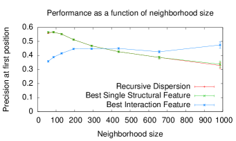
We begin by considering the size of the network neighborhood of the user $u$; recall that in our data, this size ranges from 50 to 2000. We find that recursive dispersion performs well across this full range: Figure 8 shows that, while performance is best when the neighborhood size is around 100 nodes (56%), it only drops moderately (to 33%) as the neighborhood size increases by an order of magnitude to 1000 nodes. This decline is quite small compared to the decline of the baseline that simply guesses a node uniformly at random, which would decrease in performance by a factor of $10$ (from $1/100$ to $1/1000$). The modest decline of recursive dispersion may reflect the ways in which larger neighborhoods are also more informative about a user’s full set of off-line relationships, which helps offset the considerably increased number of options for identifying the relationship partner. Furthermore, recursive dispersion is the highest-performing structural measure among those considered for every range of neighborhood sizes except the extremes (50 to 100, and above 1000); at the extremes, the (non-recursive) normalized dispersion is slightly better, although even here the recursive measure is within the margin of error of the best. Note that the median neighborhood size in our dataset is 205.

The benefits of large neighborhoods are reflected even more clearly when we consider the performance of interaction features — their performance tends to be approximately constant, or even increasing, as a function of neighborhood size. To elaborate on the arguments discussed above for how a larger neighborhood may help performance, we make two further observations. First, users with large neighborhoods also tend to be more active, and thus the relative variance of the interaction signals is smaller. Second, despite their large neighborhoods, previous analysis [21] has shown that the number of relationships that are actively maintained grows slowly in the total neighborhood size, and so the number of plausible candidates for the relationship partner grows more slowly than the pure neighborhood size would suggest.

type	max.	max.	all.	all.	comb.
	struct.	inter.	struct.	inter.
all	0.506	0.415	0.531	0.560	0.705
married	0.607	0.449	0.624	0.526	0.716
engaged	0.446	0.442	0.472	0.615	0.708
relationship	0.344	0.441	0.377	0.605	0.682

Figure 10: The performance of methods based on machine learning that combine sets of features. The first two columns show the highest performing individual structural and interaction features; the third and fourth columns show the highest performance of machine learning classifiers that combine structural and interaction features respectively; and the fifth column shows the performance of a classifier that combines all structural and interaction features together.

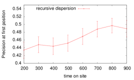
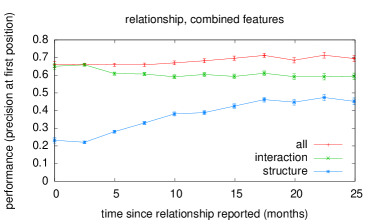
We also consider a user’s time on site — the number of days since they joined Facebook. This is strongly correlated with neighborhood size, since users continue acquiring friendship links over their time on Facebook, and it is also correlated with the time since the relationship was first reported. (As we will see later in Figure 11, performance varies as a function of this latter quantity as well.) To understand whether there is any effect of a user’s time on site beyond its relation to these other parameters, we consider a subset of users where we restrict the neighborhood size to lie between 100 and 150, and the time since the relationship was reported to lie between 100 and 200 days. Figure 9 shows that for this subset, there is a weak increase in performance as a function of time on site; while the effect is not strong, it points to a further source of enhanced performance for users with mature neighborhoods.

Figure 11: Performance at identifying partners for users who are (top row) married and (bottom row) in a relationship, as a function of the time since the relationship was reported on Facebook. In the two figures in the left-hand column, the four measures from Figure 4 are used individually. Here the structural measures have higher performance on older relationships, while the profile viewing feature has lower performance on older relationships; the profile viewing feature outperforms recursive dispersion for relationships reported recently, with the relative performance crossing at approximately one year. In the two figures in the right-hand column, the performance as a function of time is shown for prediction rules constructed using machine learning on a large set of features. Separate curves show the performance using only structural features, only interaction features, and when using the union of the two. Structural features peform best on older marriages, while interaction features perform best on new relationships.

5 Combining Features using Machine Learning

Different features may capture different aspects of the user’s neighborhood, and so it is natural to ask how well we can predict partners when combining information from many structural or interaction features via machine learning.

Machine Learning Techniques.

For our machine learning experiments, we compute $48$ structural features and $72$ interaction features for all of the nodes in the neighborhoods from our primary dataset. This gives us a total of approximately 18.7 million labeled instances with $120$ features each — each instance consists of a node $v$ in a neighborhood $G_{u}$, with a positive label indicating $v$ is the partner of $u$, or a negative label indicating $v$ is not.

The 48 structural features are the absolute and normalized dispersion based on six distinct distance functions defined for Figure 6, as well as the recursive versions using iterations 2 through 7 (recall that the recursive dispersion corresponds to the third iteration, and is hence included). The 72 interaction features represent a broad range of properties including the number of photos in which $u$ and $v$ are jointly tagged, the number of times $u$ has viewed $v$’s profile over the last 30, 60, and 90 days, the number of messages sent from $u$ to $v$, the number of times that $u$ has ‘liked’ $v$’s content and vice versa, and measures based on a number of forms of interaction closely related to these.

To improve the performance of the learning algorithms, we transformed each of the $120$ features into $4$ different versions: (a) the raw feature, (b) a normalized version of the feature with mean 0 and standard deviation 1, (c) a rank version of the feature (where the individual with highest score on this feature has rank 1, and other individuals are sorted in ascending rank order from there), and (d) a rank-normalized version where we divide (c) by total number of friends a user has. Thus, the input to our machine learning algorithms has $480$ features derived from $120$ values per instance. In addition to the full set of features, we also compute performance using only the structural features, and only the interaction features.

We performed initial experiments with different machine learning algorithms and found that gradient tree boosting [13] out-performed logistic regression, as well as other tree-based methods. Thus, all of our in-depth analysis is conducted with this algorithm. In our experiments, we divide the data so that 50% of the users go into a training set and 50% go into a test set. We perform 12 such divisions into sets A and B; for each division we train on set A and test on B, and then train on B and test on A. For each user $u$, we average over the 12 runs in which $u$ was a test user to get a final prediction.

Performance of Machine Learning Methods.

We find (Figure 10) that by using boosted decision trees to combine all of the $48$ structural features we analyzed, we can increase performance from $50.8\%$ to $53.1\%$. We can use the same technique to predict relationships based on interaction features. We find that, overall, interaction features perform slightly better than structural features (56.0% vs. 53.1%), though for married users, structural features do much better (62.4% vs. 52.6%). In addition, on all categories we find that the combination of interaction features and structural features significantly outperforms either on its own. When combining all features with boosted trees, the top predicted friend is the user’s partner 70.5% of the time.

Machine Learning to Predict Relationship Status.

Earlier we noted that our focus is on the problem of identifying relationship partners for users where we know that they are in a relationship. It is natural to ask about the connection to a related but distinct question — estimating whether an arbitrary user is in a relationship or not.

This latter question is quite a different issue, and it seems likely to be more challenging and to require a different set of techniques. To see why, consider a user $u$ who has a link of high dispersion to a user $v$. If we know that $u$ is in a relationship, then $v$ is a good candidate to be the partner. But our point from the outset has been that methods based on dispersion are useful more generally to identify individuals $v$ with interesting connections to $u$, in the sense that they have been introduced into multiple foci that $u$ belongs to. A user $u$ can and generally will have such friends even when $u$ is not in a romantic relationship. For example, Figure 5 suggests that family members often have this property, and this can apply to users who are not in romantic relationships as well as to users in such relationships. Thus, simply knowing that $u$ has links of high dispersion should not necessarily give us much leverage in estimating whether $u$ is in a relationship.

We now describe some basic machine-learning results that bear out this intuition. We took approximately 129,000 Facebook users, sampled uniformly over all users of age at least 20 with between 50 and 2000 friends. 40% of these users were single, while the remaining were either in a relationship, engaged, or married. We attempt two different prediction tasks: first, determining whether a user is in any sort of a relationship; and second, an easier task in which we look only at single and married users, and attempt to determine which category a user belongs to. We consider three different sets of features for these tasks: (i) demographic features (age, gender, country, and time on site); (ii) structural features of the network neighborhood, based on the definitions presented earlier; and (iii) the union of these two sets.

Figure 12 shows the performance on these tasks. Because age is a powerful feature for predicting relationship status, demographic features do well. Network features are not as strong, reflecting the notion discussed above that even users not in relationships have friends with similar structural properties. Despite this, network features convey non-trivial information about relationship status; they perform significantly above baseline prediction on their own, and add predictive power to demographic features. Of the network features, the maximum normalized dispersion (where the maximum is taken over all of the user’s friends) has the highest feature importance.

Task	baseline	demo.	network	both
Single vs. Any Rel.	59.8%	67.9%	61.6%	68.3%
Single vs. Married	56.6%	78.0%	66.1%	79.0%

Figure 12: Performance on predicting relationship status. Baseline accuracy comes from predicting the more common class in each of the classification tasks. Demographic features seem more important, but network features also provide incremental improvement.

6 Temporal Properties

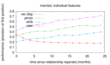
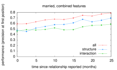
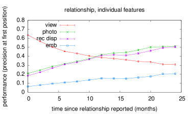
We now explore some of the ways in which these measures change over time. We first consider how performance varies based on the time since the relationship was first reported by the user — an approximate surrogate for the age of the relationship itself, although the relationship may clearly have existed for some time before it was reported (especially in the case of users who are already in a relationship when they join Facebook). We find (Fig. 11) that the structural measures are more accurate on older relationships than on newer ones, while the profile viewing feature is less accurate; in effect, the structural signature of the relationship needs time to ‘burn in’ to the network, while the interaction level via profile viewing is high almost immediately. For married users, recursive dispersion has the highest performance across the full time range, but for users in a relationship, an interesting crossover occurs: for relationships less than a year old, the profile viewing featured produces the highest performance, and then recursive dispersion and photo viewing surpass it at approximately one year. This illustrates a trade-off between a decreasing level of observation as a relationship goes on, contrasted with an increasing level of dispersion in the network as the link structure adapts around the two individuals.

Figure 13: The performance of embeddedness and normalized and recursive dispersion increase as two people approach the point at which they announce their relationship status as ‘married’ (at time 0).

Figure 14: For different subsets of users, we can evaluate their transition probability from the status ‘in a relationship’ to the status ‘single’ over a 60-day period. These transition probabilities are shown as a function of both normalized and recursive dispersion, separately for relationships that are 2-4 months old and for relationships that are 6-8 months old. The transition probabilities decrease monotonically, and by significant factors, for users with high normalized or recursive dispersion to their respective partners.

Figure 15: We plot the transition probability from ‘in a relationship’ to ‘single’ as a function of the age of the relationship, separately for relationships on which recursive dispersion correctly identifies the partner and those on which it does not. The transition probability is significantly higher when recursive dispersion fails to recognize the partner.

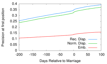
Next, we ask how these measures change over time in the period leading up to a change in relationship status. For this purpose, we take a random sample of $29000$ married users whose relationship went through a succession of stages that were all reported on Facebook — first in a relationship, next engagement, and then (after a period of at least a month of engagement) marriage. For each user $u$ in the sample, we compute embeddedness as well as normalized and recursive dispersion for all users in $G_{u}$ as a function of time, declaring time $0$ for $u$ to be the moment at which $u$’s marriage was reported. For a given network measure $m$, we then let $f_{m}(t)$ denote the fraction of instances in which $u$’s (future or current) spouse scores highest with respect to $m$. We see (Fig. 13) that normalized and recursive dispersion rise quickly to the point of marriage, while embeddedness not only has lower performance but also rises more slowly. When both embeddedness and recursive dispersion eventually identify the spouse correctly, recursive dispersion does so an average of approximately 80 days sooner; in the analogous comparison between normalized and recursive dispersion, the latter identifies the spouse an average of approximately 10 days sooner.

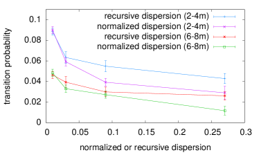
Finally, we consider the persistence of relationships [20]. Given the effectiveness of these measures in detecting partners, is it also the case that partnerships that are more strongly identified by the measures are also more ‘robust,’ in the sense that they are more likely to persist over time? We address this question by considering those users in our sample who listed themselves as being in a relationship (rather than married or some other relationship status, a set of roughly 400,000 individuals), and seeing which of them lists their relationship status as ‘single’ 60 days later. We perform these analyses on subsets of the data on which all relationships have roughly the same age since they were reported on Facebook, and on which all users were approximately the same age, to separate these effects from the underlying structural parameters. We find (Fig. 14) that a user whose partner has a high normalized or recursive dispersion is significantly less likely to transition to ‘single’ status over this time period.

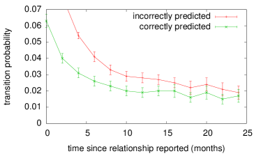
We can view the persistence of relationships in a closely related way by comparing relationships on which recursive dispersion correctly identifies the partner to those on which it does not. We find (Fig. 15) that relationships on which recursive dispersion fails to correctly identify the partner are significantly more likely to transition to ‘single’ status over a 60-day period. This effect holds across all relationship ages and is particularly pronounced for relationships up to 12 months in age; here the transition probability is roughly 50% greater when recursive dispersion fails to recognize the partner.

7 Beyond Immediate Neighborhoods

All of the network measures discussed above are based on the immediate 1-hop neighborhoods of individuals. It is interesting to consider how accurate more expansive methods might be, if they take the broader structure of the network into account. Because many individuals have 2-hop neighborhoods with hundreds of thousands of nodes, doing this is computationally challenging, and we must come up with heuristics to make it feasible.

Our approach is to take a single structural measure, recursive dispersion, and filter down to an individual’s top 20 friends as ranked by this metric. We then compute the network measures discussed above in the (1-hop) neighborhoods of each of these 20 people. To evaluate a given friend $v$ as the potential partner of $u$, we can then use the measures computed in $u$’s neighborhood and also in $v$’s. We find that the simple heuristic of taking $u$’s top 20 friends with respect to $rec(u,v)$, and then ranking them by $\min(rec(u,v),rec(v,u))$, improves performance by about $6\%$ to $0.534$. This performs almost as well as more complex models, and confirms the intuitive result that relationship partners are best found by looking for pairs of people who have high scores in both directions.

8 Conclusion

Understanding the structural roles of significant people in on-line social network neighborhoods is a broad question that requires a combination of different approaches. Here we have considered this issue in the context of romantic partners, and have identified a novel network measure, dispersion, that provides a powerful method for recognizing the structural positions occupied by such partners from network data alone.

Drawing on the theory of social foci [10], we have argued that dispersion is a structural means of capturing the notion that a friend spans many contexts in one’s social life — either because they were present through multiple life stages, or because they have been systematically introduced into multiple social circles. This suggests why it is not only spouses or romantic partners who exhibit high dispersion, but also family members — dispersion identifies people who span foci.

There are several applications where measures based on dispersion may play a role. For estimating which types of content from friends will be most engaging to a user [1], identifying individuals with this focus-spanning property can be useful for assessing their properties both as producers and consumers of content from different parts of a user’s network neighborhood. And for organizing neighborhoods into distinct clusters or circles [23, 25], dispersion can help identify ‘hard-to-categorize’ individuals who may need manual annotation from a user — high dispersion arises precisely because a friend doesn’t naturally fit into the obvious categories

Beyond these specific applications, our measures suggest new perspectives on basic questions in social network analysis. Overall, the notion that our mutual friends with a person may be clustered in a single context or may alternately span multiple contexts offers a novel type of trade-off in the study of tie strength. Certain important types of strong ties — including romantic and family relations — connect us to people who belong to multiple parts of our social neighborhood, producing a set of shared friends that is not simply large but also diverse, spanning disparate portions of the network and hence correspondingly sparse in their internal connections. In this way, the notion of dispersion combines concepts of network closure[16, 6] (since there must be mutual network neighbors to bridge) and brokerage between groups[5] (since the two ends of a link with large dispersion are jointly acting as brokers between disconnected mutual neighbors). The success of the measures resulting from this notion suggests some of the ways in which closure and brokerage are intertwined in the structure of strong ties.

The analysis shows how these classes of strong ties produce an extremely clear structural signature, but subtle network measures different from the standard formulations are needed to extract this signature. Crucial aspects of our everyday lives may be encoded in the network structure among our friends, provided that we look at this structure under the right lens.

Acknowledgments.

We thank Matt Brashears, Ben Cornwell, Lillian Lee, Michael Macy, Cameron Marlow, Sendhil Mullainathan, Brian Rubineau, and Johan Ugander for valuable discussions, and the Simons Foundation and NSF for support.

9 Appendix: Mathematical Properties of the Recursive Dispersion

This section provides some motivation and further mathematical detail related to the recursive dispersion, to help isolate the ingredients that make up its functional form.

First, fix a distance function $d_{v}$ on the graph $G-\{u,v\}$. We first note that if we assign a value $x_{s}=1$ to each node $s$ in $G_{u}$, then $\sum_{s,t\in C_{uv}}d_{v}(s,t)x_{s}x_{t}$ is precisely the dispersion of $v$, since it is a sum over all pairwise distances in $C_{uv}$. Hence,

$$\frac{\sum_{s,t\in C_{uv}}d_{v}(s,t)x_{s}x_{t}}{emb(u,v)}$$

is the normalized dispersion.

The premise underlying the recursive dispersion is to elevate $x_{v}$ when $u$ and $v$ act as intermediaries between many node pairs $s$ and $t$ that, recursively, have large values of $x_{s}$ and $x_{t}$. A simple way to carry out this idea would be to define an iteration in which $x_{v}$ is updated to be

$$x_{v}~{}\longleftarrow~{}\frac{\sum_{s,t\in C_{uv}}d_{v}(s,t)x_{s}x_{t}}{emb(u,v)},$$ (1)

directly using the functional form of the normalized dispersion. The problem with this approach on the graphs $G_{u}$ that we have in the data is that the sum in the numerator is equal to $0$ for many nodes $v$. This in turn means that even more nodes will acquire a $0$ value in subsequent iterations; the end result is that very few nodes end up with a positive value $x_{v}$, and this would hurt the performance in identifying partners.

As a result, it is useful to have a mechanism that continuously introduces non-zero weight into the system. As a working guideline for how to do this, we would like the first iteration to produce values $x_{v}$ whose sorted order agrees with the order of values according to normalized dispersion, so that subsequent iterations can be viewed as building from this measure. We would also like additional terms in the numerator to be quadratic, to match the quadratic degree of the existing terms in the numerator of (1). Adding $\sum_{w\in C_{uv}}x_{w}^{2}$ to the numerator achieves these two properties in a simple way — it is quadratic, and in the first iteration it is equal to $emb(u,v)$, and hence is canceled by the denominator. This gives us the functional form that we use as the recursive dispersion:

$$x_{v}\longleftarrow\frac{\sum_{w\in C_{uv}}x_{w}^{2}+2\sum_{s,t\in C_{uv}}d_{v}(s,t)x_{s}x_{t}}{emb(u,v)}.$$ (2)

Depending on the structure of $G_{u}$, the right-hand side of (2) can simplify in several instructive ways. In what follows, we will also write $emb(u,v)$ in an equivalent form as $|C_{uv}|$.

• First, suppose $G_{u}$ has the property that $d_{v}(s,t)=1$ whenever $s$ and $t$ belong to the set $C_{uv}$. For example, with our distance function $d_{v}$, this would hold if the graph $G_{u}-\{u\}$ had no cycle of length less than $5$; in this case, for any $v$ and any $s,t\in C_{uv}$, there could be no common neighbor of $s$ and $t$ other than $u$ and $v$, and so $d_{v}(s,t)=1$. In this case, the iteration in (2) becomes

  $$x_{v}\longleftarrow\frac{\sum_{w\in C_{uv}}x_{w}^{2}+2\sum_{s,t\in C_{uv}}x_{s}x_{t}}{emb(u,v)}=\frac{\left(\sum_{w\in C_{uv}}x_{w}\right)^{2}}{|C_{uv}|}$$ (3)

  and so the values evolve according to an iteration that simply sums values at neighboring nodes and then squares the sum (with normalization).

• Alternately, suppose $G_{u}$ has the property that $d_{v}(s,t)=0$ for all pairs of nodes $s$ and $t$ that belong to the same set $C_{uv}$. For example, again using our distance function $d_{v}$, this would be true if every pair of nodes at distance $2$ in $G_{u}$ had at least two common neighbors other than $u$. In this case, if in a given iteration we have $x_{s}=c$ for all $s$, then in the next iteration

  $$x_{v}\longleftarrow\frac{\sum_{w\in C_{uv}}x_{w}^{2}}{emb(u,v)}=\frac{c^{2}|C_{uv}|}{|C_{uv}|}=c^{2},$$ (4)

  and so all values remain equal to each other. Thus, for such a $G_{u}$, all nodes have the same recursive dispersion.

These two special cases represent different conceptual extremes, and most graphs will lie in between. It is an interesting open question to understand the convergence properties of recursive dispersion in arbitrary graphs.

References

- [1] Backstrom, L., Kleinberg, J. M., Lee, L., and Danescu-Niculescu-Mizil, C. Characterizing and curating conversation threads: expansion, focus, volume, re-entry. Proc. 6th ACM WSDM, 2013.
- [2] Bearman, P., Moody, J., and Stovel, K. Chains of affection: The structure of adolescent romantic and sexual networks. American J. Sociology 110, (2004).
- [3] Blondel, V. D., Guillaume, J.-L., Lambiotte, R., and Lefebvre, E. Fast unfolding of communities in large networks. Journal of Statistical Mechanics (2008).
- [4] Bott, E. Family and Social Network: Roles, Norms, and External Relationships in Ordinary Urban Families. Tavistock Press, 1957.
- [5] Burt, R. S. Structural Holes: The Social Structure of Competition. Harvard University Press, 1992.
- [6] Coleman, J. S. Social capital in the creation of human capital. American J. Sociology 94, (1988).
- [7] Cornwell, B. Spousal network overlap as a basis for spousal support. J. Marriage and Family 74 (2012).
- [8] Eagle, N., Pentland, A. S., and Lazer, D. Inferring friendship network structure by using mobile phone data. Proc. Natl. Acad. Sci. USA 106, (2009).
- [9] Farnham, S., and Churchill, E. F. Faceted identity, faceted lives: social and technical issues with being yourself online. In Proc. 14th ACM CSCW (2011).
- [10] Feld, S. L. The focused organization of social ties. American J. Sociology 86, (1981).
- [11] Felmlee, D. H. No couple is an island: A social network perspective on dyadic stability. Social Forces 79 (2001).
- [12] Fischer, C. To Dwell Among Friends. U. Chicago, 1982.
- [13] Friedman, J. H. Greedy function approximation: A gradient boosting machine. Ann. Statistics 29 (2000).
- [14] Gilbert, E., and Karahalios, K. Predicting tie strength with social media. In Proc. 27th ACM Conference on Human Factors in Computing Systems (2009), 211–220.
- [15] Granovetter, M. The strength of weak ties. American Journal of Sociology 78 (1973), 1360–1380.
- [16] Granovetter, M. Economic action and social structure: The problem of embeddedness. Amer. J. Soc. 91(1985).
- [17] Jones, J. J., Settle, J. E., Bond, R. M., Fariss, C. J., Marlow, C., and Fowler, J. H. Inferring tie strength from online directed behavior. PLoS ONE 8 (2013)
- [18] Kalmijn, M. Shared friendship networks and the life course. Social Networks 25 (2003).
- [19] Kossinets, G., and Watts, D. Empirical analysis of an evolving social network. Science 311 (2006), 88–90.
- [20] Le, B., Dove, N. L., Agnew, C. R., Korn, M. S., and Mutso, A. A. Predicting nonmarital romantic relationship dissolution: A meta-analytic synthesis. Personal Relationships 17, 3 (Sept. 2010), 377–390.
- [21] Marlow, C., Byron, L., Lento, T., and Rosenn, I. Maintained relationships on Facebook, 2009. On-line at http://overstated.net/2009/03/09/maintained-relationships-on-facebook The cited figures and results from this work, including Figure 1, are reproduced with permission in the book Networks, Crowds, and Markets (D. Easley and J. Kleinberg, Cambridge University Press, 2010.).
- [22] Marsden, P. V., and Campbell, K. E. Measuring tie stength. Social Forces 63, 2 (Dec. 1984), 482–501.
- [23] McAuley, J. J., and Leskovec, J. Learning to discover social circles in ego networks. Proc. NIPS (2012).
- [24] McPherson, M., Smith-Lovin, L., and Brashears, M. E. Social isolation in America: Changes in core discussion networks over two decades. Am. Soc. Rev. 71 (2006).
- [25] Min, J.-K., Wiese, J., Hong, J. I., and Zimmerman, J. Mining smartphone data to classify life-facets of social relationships. In Proc. 16th ACM CSCW (2013).
- [26] Newman, M. E. J. The structure and function of complex networks. SIAM Review 45 (2003), 167–256.
- [27] Onnela, J.-P., Saramaki, J., Hyvonen, J., Szabo, G., Lazer, D., Kaski, K., Kertesz, J., and Barabasi, A.-L. Structure and tie strengths in mobile communication networks. Proc. Natl. Acad. Sci. USA 104 (2007).
- [28] Zhao, X., Sosik, V. S., and Cosley, D. It’s complicated: how romantic partners use Facebook. In Proc. 30th ACM Conf. Human Factors in Computing Systems (2012).