The Physical Conditions, Metallicity and Metal Abundance Ratios In a Highly Magnified Galaxy at z $=$ 3.6252 ^∗

Abstract

We present optical and near-IR imaging and spectroscopy of SGAS J105039.6$+$001730, a strongly lensed galaxy at z $=$ 3.6252 magnified by $>$ 30$\times$, and derive its physical properties. We measure a stellar mass of log(M_∗/M_⊙) $=$ 9.5 $\pm$ 0.35, star formation rates from [O II]$\lambda$$\lambda$3727 and H-$\beta$ of 55 $\pm$ 25 and 84 $\pm$ 24 M_⊙ yr^-1, respectively, an electron density of n${}_{e}\leq$ 10³ cm^-2, an electron temperature of T${}_{e}\leq$ 14000 K, and a metallicity of 12 $+$ log(O/H) $=$ 8.3 $\pm$ 0.1. The strong C III]$\lambda$$\lambda$1907,1909 emission and abundance ratios of C, N, O and Si are consistent with well-studied starbursts at z $\sim$ 0 with similar metallicities. Strong P Cygni lines and He II$\lambda$1640 emission indicate a significant population of Wolf-Rayet stars, but synthetic spectra of individual populations of young, hot stars do not reproduce the observed integrated P Cygni absorption features. The rest-frame UV spectral features are indicative of a young starburst with high ionization, implying either 1) an ionization parameter significantly higher than suggested by rest-frame optical nebular lines, or 2) differences in one or both of the initial mass function and the properties of ionizing spectra of massive stars. We argue that the observed features are likely the result of a superposition of star forming regions with different physical properties. These results demonstrate the complexity of star formation on scales smaller than individual galaxies, and highlight the importance of systematic effects that result from smearing together the signatures of individual star forming regions within galaxies.

1. Introduction

The accumulation of stellar mass and metallicity in galaxies at high redshift involves complex interactions between several astrophysical processes, including star formation, winds and outflows, and gas accretion. In the current prevailing paradigm metal-poor gas is accreted from the intergalactic medium (IGM) and fuels star formation, which enriches the interstellar medium (ISM) with metals and generates galaxy-scale winds. This general picture provides a broad framework for understanding how galaxies build up their mass and metal content, but the details of how accretion, star formation, enrichment, and outflows are physically regulated remain poorly understood.

The rest-frame ultraviolet spectra of star forming galaxies include a wealth of diagnostics that constrain the properties of massive stars, the elemental abundances and physical properties of the nebular gas that those stars ionize, and the galaxy-scale outflows that they power. Rest-frame near-infrared spectra provide complementary measurements of the physical properties of the ionized nebular line-emitting regions. However, the observational data at z $>$ 3 remains extremely limited; the current challenge is to obtain good data for faint, distant galaxies.

Table 1Summary of Spectroscopic Observations

Telescope	Instrument	UT Date	Disperser	Filter	Wavelengths (Å)	FWHM (Å)
Magellan-I	FIRE	Jun 11,12 2011	echelle	—	10000-24000	2.8-6.1
Gemini-North	GMOS	Mar 29 2012	R400 grating	OG515	5600-9800	8.2
Magellan-I	IMACS	Mar 17 2013	200 l/mm grism	—	4800-9800	9.4
Magellan-II	MagE	May 06 2013	echellette 175 l/mm	—	3500-8500	1.2-2.0

Photometry is relatively inexpensive, but reveals only limited constraints on the internal properties of galaxies. Spectroscopy provides significantly more information, but high S/N spectra of individual high redshift field galaxies are an expensive use of current instrumentation on larger-aperture telescopes (e.g., Erb et al., 2010), and are limited to sampling the brightest (i.e., atypical) field galaxies. Stacking analyses of low signal-to-noise (S/N) spectra are useful for understanding the average properties of galaxies (e.g., Shapley et al., 2003; Jones et al., 2012), but sample neither the variations between galaxies nor the variations between regions within individual galaxies. Strong gravitational lensing provides a means by which the detailed physical properties of distant galaxies can be studied at high S/N. Galaxies that are highly magnified by massive foreground structures – typically galaxy groups/clusters – have their flux boosted by factors of $\gtrsim$ 10. Observations of these lensed sources with current facilities provide data that will only be matched, at best, by future generations of 30m class telescopes.

Figure 1.— Color composite image of the core of strong lensing cluster SDSS J1050+0017 using HST/WFC3 F110W/F606W/F390W assigned as R/G/B. We have labeled both SGAS J105039.6$+$001730 and its confirmed counter image, and provided zoom insets of the regions around both the arc and counter image. A compass in the upper left corner indicates North (long) and East (short), and the image scale is marked in the upper right corner.

The exploitation of strong lensing to conduct high S/N studies of intrinsically faint galaxies at high redshift dates back to MS 1512-cB58 (“cB58” Yee et al., 1996), a z $=$ 2.73 Lyman Break Galaxy (LBG) that is magnified by a foreground galaxy cluster by a factor of $\sim$ 30 (Seitz et al., 1998). Follow-up observations of cB58 yielded a high S/N spectra that revealed a tremendous level of detail about the chemical composition and state of the ISM (Pettini et al., 2000; Teplitz et al., 2000; Pettini et al., 2002). In recent years several “cB58-like” strongly lensed z $\sim$ 2-3 galaxies have been discovered (Fosbury et al., 2003; Cabanac et al., 2005; Allam et al., 2007; Belokurov et al., 2007; Smail et al., 2007; Diehl et al., 2009; Lin et al., 2009; Koester et al., 2010; Wuyts et al., 2010), and efforts to target these apparently bright (but intrinsically faint) galaxies for optical and NIR spectroscopy with large ground-based telescopes are accelerating. The lensing magnification allows for high quality spectroscopy from which the detailed physical properties and abundances can be derived (Hainline et al., 2009; Quider et al., 2009; Yuan & Kewley, 2009; Bian et al., 2010; Dessauges-Zavadsky et al., 2010; Erb et al., 2010; Jones et al., 2010; Quider et al., 2010; Dessauges-Zavadsky et al., 2011; Rigby et al., 2011; Wuyts et al., 2012a, b; Jones et al., 2013a; Stark et al., 2013; Shirazi et al., 2013; James et al., 2014). Observations of emission line properties of fainter strongly lensed galaxies have also enabled measurements that push farther down the faint end of the luminosity function, deeper into the mass function, and out to higher redshifts (Bayliss et al., 2010; Richard et al., 2011; Christensen et al., 2012b, a; Wuyts et al., 2012a, b; Jones et al., 2013b).

In this paper we present a multi wavelength analysis of SGAS J105039.6$+$001730, a LBG at z $=$ 3.6252 that is strongly lensed by a foreground galaxy cluster at z $=$ 0.593 $\pm$ 0.002; the giant arc is highly magnified and has an apparent AB magnitude of F606W $=$ 21.48 (Figure 1). This is the most distant galaxy for which a detailed study of the properties of massive stars and the inter-stellar medium (ISM) has been performed. SGAS J105039.6$+$001730 was discovered as a part of the Sloan Giant Arcs Survey (SGAS; M. D. Gladders et al. in prep), an on-going search for galaxy group and cluster scale strong lenses in the Sloan Digital Sky Survey (SDSS; York et al., 2000). The full SGAS sample includes hundreds of strong lenses, many of which have been published in a variety of cosmological and astrophysical analyses (Oguri et al., 2009; Koester et al., 2010; Bayliss et al., 2010, 2011a, 2011b; Gralla et al., 2011; Oguri et al., 2012; Bayliss, 2012; Dahle et al., 2013; Wuyts et al., 2012a, b; Gladders et al., 2013; Blanchard et al., 2013). SGAS J105039.6$+$001730 appears near the core of a strong lensing cluster that was first published by Oguri et al. (2012).

This paper is organized as follows: in $\S$ 2 we summarize the follow-up observations of SGAS J105039.6$+$001730 that inform this work, including both space- and ground-based imaging, as well as extensive optical and NIR spectroscopy. In $\S$ 3 we review the analysis methods that we apply to the available data: spectral line profile measurements, systemic redshifts, strong lens modeling of the lens-source system, and photometry. $\S$ 4 includes the derivation of the detailed physical properties of SGAS J105039.6$+$001730, including stellar mass constraints from spectral energy distribution (SED) fitting, as well as the internal redding/extinction, star formation rates, electron density & temperature, metallicity, and abundance ratios. In $\S$ 5 we discuss the physical picture that emerges for SGAS J105039.6$+$001730 given the available data, and we place it in the context of other studies of high redshift galaxies. Finally, $\S$ 6 contains a summary of our analysis and its implications.

All magnitudes presented in this paper are in the AB system, based on calibration against the SDSS. We use a solar oxygen abundance Z_⊙: 12 $+$ log(O/H) $=$ 8.69 (Asplund et al., 2009). All cosmologically dependent calculations are made using a standard flat $\Lambda$ cold dark matter ($\Lambda$CDM) cosmology with $H_{0}=70$ km s^-1 Mpc^-1, and matter density $\Omega_{M}=0.27$ as preferred by observations of the Cosmic Microwave Background, supernovae distance measurements, and large scale structure constraints (Komatsu et al., 2011; Reichardt et al., 2013).

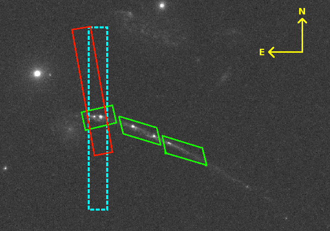
Figure 2.— HST/WFC3-IR F606W image of SGAS J105039.6$+$001730 with slits over-plotted for each of the follow-up spectroscopic observations described in Section 2. The three smaller green slits indicate the positions of slits placed on the arc in the GMOS nod-and-shuffle mask. The shorter GMOS slit was observed at both the pointing and nod positions of the N&S observation, and therefore received twice the integration time as the other two tilted slits (this slit also covers the brightest part of the arc, and therefore dominates the signal in the final stacked GMOS spectrum). The longest cyan slit (dashed lines) indicates the position of the MagE slit, and the single long, tilted red slit indicates one of the two AB nod positions of the FIRE slit.

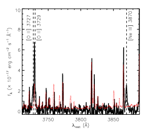
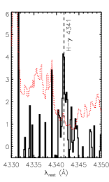
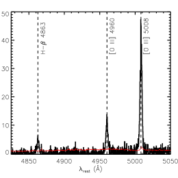
Figure 3.— Selected regions of the FIRE spectrum with emission lines indicated by vertical dashed lines and labeled, and the error array is over plotted as the dotted red line. Left: FIRE spectrum covering the rest-frame wavelength range $\Delta\lambda=$ 3710-3890-Å. Middle: FIRE spectrum covering the rest-frame wavelength range $\Delta\lambda=$ 4330-4350Å. Right: FIRE spectrum covering the rest-frame wavelength range $\Delta\lambda=$ 4825-5050Å.

2. Observations

2.1. Imaging

2.1.1 Subaru/SuprimeCam

The field centered on SGAS J105039.6$+$001730 was observed with the Subaru telescope and the SuprimeCam instrument on UT Apr 7, 2011. The resulting data consist of $g$-, $r$- and $i$-band imaging, with total integration times of 1200 s, 2100 s, and 1680 s in $g$, $r$, and $i$, respectively. These observations were optimized to take advantage of the large field of view of SuprimeCam ($\sim$34′$\times$27′), and were used in a combined strong$+$weak lensing analysis of the foreground lensing cluster, SDSS J1050+0017; for details of the image reductions and resulting lensing analysis we direct the reader to Oguri et al. (2012).

2.1.2 HST/WFC3

SGAS J105039.6$+$001730 was observed with the Hubble Space Telescope and the Wide Field Camera 3 using both the IR and UVIS channels on UT Apr 19-20, 2013 as a part of the GO 13003 (PI: Gladders) program. Total integration times are 1212 s, 1112 s, 2400 s, 2388 s in the F160W, F110W, F606W and F390W filters, respectively. A post flash was applied to the individual F390W exposures to reduce the impact of charge-transfer inefficiency in the WFC3 UVIS camera.

The image processing was performed using the DrizzlePac software package. Images were rescaled by re-drizzling the corrected flats with the astrodrizzle routine to a scale of 0.03″ pixel^-1 to take advantage of the finer grid made possible by our dithering pattern. The resulting images were then aligned across filters with the image taken in the F606W filter using the tweakreg function. The astrometric solutions provided by tweakreg were then propagated back to the corrected flat-fielded images using tweakback. Using astrodrizzle, the F606W flat field images were drizzled onto a new grid with a scale of 0.03″ pixel^-1, once with a drop size of 0.8 pixels, and separately again with a drop size of 0.5. We found that a drop size of 0.5 for the IR camera and 0.8 for the UVIS camera provide the best sampling of the point spread function into our common pixel scale of $0\farcs 03$. The resulting image was used as a reference grid for the re-drizzling of the images taken in the three remaining filters using the same scale and drop size and the updated astrometric solutions.

The WFC3 images were further processed to correct for IR ‘Blobs’ not removed by the standard WFC3 pipeline flat-fields. These artifacts appear as small regions of reduced sensitivity due to dust particles contaminating the steering mirror that directs light into the WFC3 IR channel. We used object-masked individual frames in each IR filter, from the entire large HST GO program, to generate a sky flat for each filter. Though the IR blob artifacts are apparent in each flat, the raw flats are significantly contaminated from residual flux from real objects, and so we used GALFIT Peng et al. (2010) to create a model of each IR blob as the sum of a few Gaussian components. This model is then used to flat-field the artifacts on each individual IR frame. UVIS flats were corrected for charge transfer inefficiencies using the CTE correction tool provided by STScI.

2.1.3 Spitzer/IRAC

Observations of SGAS J105039.6$+$001730 were obtained in the 3.6$\mu$m and 4.5$\mu$m channels as a part of Spitzer program #70154 (PI: Gladders). Total integration times were 1200 s, taken during the warm Spitzer/IRAC mission. The data were reduced with the MOPEX software distributed by the Spitzer Science Center and drizzled to a pixel scale of 0.6″ pixel^-1.

2.2. Spectroscopy

A summary of spectroscopic observations used in this work is shown in Table 1. In the following sections we describe the spectroscopic data and their reduction.

2.2.1 Magellan/FIRE

Near-infrared spectroscopic observations were obtained with the Folded-port InfraRed Echellete (FIRE) instrument (Simcoe et al., 2013) on the Magellan-I (Baade) telescope. SGAS J105039.6$+$001730  was observed on two nights, UT 2011-06-11 and 2011-06-12. A pair of frames with individual integrations times of 602 s were obtained each of the two nights, for a total integration of 2410 s. The echelle grating and the 1.0 ″ slit were used, resulting in spectral resolution of R$=$3600 (83 km s^-1). The position of the FIRE slit is shown in Figure 2.

The A0 V star HD 96781 was observed as a standard star for purposes of fluxing and telluric correction. The star was observed immediately before each pair of science frames; the star was located 14 degrees from the science target, with sec(Z) airmass that differed by less than 0.2.

FIRE data were reduced using the FIREHOSE data reduction pipeline tools, which were written in IDL by R. Simcoe, J. Bochanski, and M. Matejek, and kindly provided to FIRE users by the FIRE team.

The FIRE pipeline uses lamp flat-fields to correct the pixel-to-pixel variation and sky flats to correct the illumination. The wavelength solution is fit using OH sky lines, and a two dimensional model of the sky is iteratively fit and subtracted following Kelson (2003). The object spectrum is extracted using a spatial profile fit to the brightest emission line, and a flux calibration and corrected for telluric absorption correction are applied using the method of Vacca et al. (2003) as implemented in an adapted version of the xtellcor routine from the SpeX pipeline. The final FIRE spectrum is a weighted average of the spectra that were extracted from the four individual exposures.

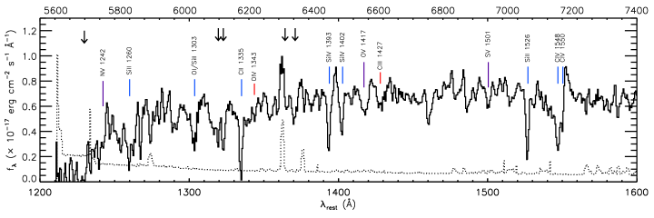
Figure 4.— Top: GMOS spectrum covering the rest-frame wavelength range $\Delta\lambda=$ 1200-1600Å. Spectral lines are indicated by type: black dashed lines are nebular emission lines, short solid red lines are stellar photospheric absorption features and medium length blue lines are ISM absorption lines, and long purple lines indicate transitions that could be either stellar photospheric or ISM (or more likely, a blend of the two). The error array is over plotted as the black dotted line, and the fit to the continuum level across the spectrum is plotted as a thin green line. The apparent emission feature that we observe at $\sim$6290Å is the result of a pernicious sky subtraction residual, and lines resulting from intervening absorption systems are indicated with downward facing arrows. Bottom: GMOS spectrum covering the rest-frame wavelength range $\Delta\lambda=$ 1600-1950Å. Lines are indicated according to the same scheme as the top panel. The N III] 1750 emission line is only detected at $\sim$2$\sigma$, but we indicate its location here because it is used later to constrain the relative nitrogen abundance.

2.2.2 Gemini/GMOS-N Nod-and-Shuffle

SGAS J105039.6$+$001730 was observed with the Gemini-North telescope and the Gemini Multi-Object Spectrograph (GMOS; Hook et al., 2004) on UT Mar 29 2012 in macro nod-and-shuffle (N&S) mode and in clear conditions with seeing $\leq$0.75″ as a part of queue program GN-2011A-Q-19. We used the R400_G5305 grating in first order with the G515_G0306 long pass filter, and the detector binned by 2 in the direction of the spectral dispersion and unbinned spatially. The N&S cycle length was 120s, chosen to reduce the number of shuffles in a given integration to mitigate charge trap effects. These observations were carried out after November 2011, and therefore used the new e2vDD detectors on GMOS-North, which provide significantly improved quantum efficiency relative to the older detectors that they replaced.

A single multi-object slit mask was used to primarily target strongly lensed background sources in the core of SDSS J1050$+$0017; the approach is identical to the data described in detail by Bayliss et al. (2011b) and we refer the reader to that paper for an in-depth description of the mask design. Four micro-slits on the mask were placed on SGAS J105039.6$+$001730, two of which covered the brightest knot in the arc at both the pointing and nod positions of the N&S observations, and two slits which covered the length of the arc at only the pointing position (see Figure 2). The total spectroscopic integration consisted of two 2400 s exposures, half of which was spent at each of the pointing and nod positions. The resulting spectra include 4800 s of total integration time on the brightest knot of SGAS J105039.6$+$001730, and 2400 s of total integration time on the fainter parts of the arc extending to the southwest. All science slits were 1″ wide, with the two slits extending along the length of the arc titled 30 degrees relative to the dispersion axis to capture as much flux as possible. Slit placements for all of our spectroscopic observations are also shown in Figure 2. The resolution of the data varies from R $\simeq$ 700-1100 (270-430 km s^-1).

Sky subtraction of N&S data is simply a matter of differencing the two shuffled sections of the detector. The GMOS data were then wavelength calibrated, extracted, stacked, flux normalized, and analyzed using a custom pipeline that was developed using the XIDL package. Flux calibration was performed using an archival observation of a single standard star and is therefore subject to pedestal offsets in the absolute flux calibration. The pipeline is almost identical to what was used by Bayliss et al. (2011b), with some updates made to account for the new e2vDD detectors.

2.2.3 Magellan/IMACS

We also observed the field centered on SGAS J105039.6$+$001730 with Magellan-I and the Inamori-Magellan Areal Camera & Spectrograph (IMACS) using the long (f/2) camera on UT Mar 17 2013 in stable conditions with seeing ranging from $\sim$0.8-1.0″, with the airmass ranging from 1.26 to 1.15. Two multi-slit masks were each observed for 3$\times$2400 s, and included several slits placed on potential counter-images of SGAS J105039.6$+$001730, as well as on other faint candidate strongly lensed background objects that were not targeted by the GMOS N&S observations. We used the 200 l/mm grism and the spectroscopic (i.e., no order blocking) filter to allow for the broadest possible wavelength coverage and sensitivity. The detector was unbinned, resulting in spectral resolution R $\simeq$ 500-1000 (300-460 km s^-1) and sensitivity over the wavelength range $\Delta\lambda=$ 4800-9800Å. The data were wavelength calibrated, bias subtracted, flat-fielded, and sky subtracted using the COSMOS reduction package designed specifically for IMACS and provided by Carnegie Observatories. The data were then extracted and stacked using custom IDL code; because the goal of these observations were redshift measurements, the extracted spectra were not precisely flux calibrated.

2.2.4 Magellan/MagE

We observed SGAS J105039.6$+$001730 with the Magellan II (Clay) telescope and the Magellan Echellette (MagE) spectrograph (Marshall et al., 2008). The observation started at May 6 2013 02:30:28 UT, and the integration time was 3600s; the MagE slit was placed on the brightest knot of the arc, which had also previously been targeted with FIRE and GMOS (Figure 2). The weather was clear, and the seeing as measured by wavefront sensing during the integration varied from 0.6 to 1.1″. The airmass rose from 1.30 to 1.57 during the observation. The target was acquired by blind-offsetting from a nearby brighter object; target acquisition was verified via the slit-viewing guider camera. The slit was 1″ by 10″ and the spectra were collected with 1$\times$1 binning resulting in a resolution of R $=$ 4100 (70 km s^-1).

The spectra were reduced using the LCO Mage pipeline written by D. Kelson. The pipeline produces an extracted, one-dimensional, wavelength-calibrated spectrum for each echelle order. The sensitivity function was computed using the IRAF tools onedspec.standard and sensfunc, using at least two observations each of the standard stars LTT 3864, EG 274, and Feige 67, at airmasses ranging from 1.02 to 1.53. We scaled the sensitivity functions to the star with the highest throughput to create a composite sensitivity function. To flux calibrate, these sensitivity functions were applied to the spectrum using the IRAF tool onedspec.calibrate. The uncertainty in the flux calibration is $\pm$20%, resulting primarily from uncertainties in the slit losses due to variable seeing over the course of long spectroscopic integrations. Overlapping orders of the echelle were combined with a weighted average to make a continuous spectrum, and then corrected to vacuum barycentric wavelength. The signal-to-noise ratio, per-pixel, of the continuum is low (rising from 0.1 at 3500 Å to 1 at 7500Å.)

2.3. GMOS vs MagE Flux Calibration

The MagE spectrum was flux-calibrated more carefully, with several standard stars during the night, whereas the GMOS flux calibration was based on a non-contemporaneous (archival) standard star observation. We therefore extract the GMOS spectrum corresponding only from the slit which covers approximately the same region that was targeted by both the MagE and FIRE observations (see Figure 2), and compare the resulting fluxed spectra against the MagE flux spectrum. In the wavelength range where both spectra have reasonable S/N (i.e., $\Delta\lambda\sim$ 6000-7000Å) the two datasets have the same continuum flux level to within $\sim$5%. Having performed this “boot-strap” flux calibration we feel secure in using the GMOS spectrum to measure line fluxes with a calibration that is accurate to within the uncertainty in the more carefully quantified MagE flux calibration ($\pm$20%).

Table 2Individual Line Redshifts

Ion	$\lambda_{rest}$	$\lambda_{obs}$	$z$	Type	Instrument
N V	1242.804	5745.68	3.62316	2/4	GMOS
N V	1242.804	5746.56	3.62386	2/4	MagE
Si II	1260.422	5826.02	3.62228	1	GMOS
O I	1302.169	6020.50	3.62344	1	MagE
O I/Si II	1303.860	6027.73	3.62299	1	GMOS
Si II	1304.370	6031.87	3.62436	1	MagE
C II	1335.480	6172.87	3.62221	1	GMOS
C II	1335.480	6172.93	3.62225	1	MagE
O IV	1343.514	6215.04	3.62596	2	GMOS
Si IV	1393.755	6444.76	3.62403	4	GMOS
Si IV	1393.755	6444.82	3.62407	4	MagE
Si IV	1402.770	6486.14	3.62381	4	GMOS
O V	1417.866	6554.22	3.62260	2/4	GMOS
C III	1427.839	6605.42	3.62617	2	GMOS
S V	1501.763	6939.89	3.62116	2/4	GMOS
Si II	1526.707	7060.20	3.62447	1	GMOS
Si II	1526.707	7061.13	3.62508	1	MagE
C IV	1548.203	7154.86	3.62139	4	GMOS
C IV	1548.203	7156.04	3.62216	4	MagE
C IV	1550.777	7170.61	3.62388	4	GMOS
C IV	1550.777	7169.76	3.62333	4	MagE
Fe II	1608.451	7438.93	3.62491	1	GMOS
Fe II	1608.451	7437.89	3.62426	1	MagE
He II	1640.420	7585.72	3.62426	3	GMOS
He II	1640.420	7586.21	3.62455	3	MagE
O III]	1660.809	7682.51	3.62577	3	GMOS
O III]	1660.809	7681.81	3.62534	3	MagE
O III]	1666.150	7707.79	3.62611	3	GMOS
O III]	1666.150	7706.46	3.62531	3	MagE
Al II	1670.788	7726.20	3.62429	1	GMOS
N IV	1718.550	7948.66	3.62521	2	GMOS
Al III	1854.716	8576.66	3.62425	1	GMOS
Al III	1862.790	8615.79	3.62521	1	GMOS
Si III]	1882.468	8708.81	3.62627	3	GMOS
Si III]	1892.030	8754.13	3.62685	3	GMOS
C III]	1907.640	8820.57	3.62381	3	GMOS
O [II]	3727.092	17237.46	3.62491	3	FIRE
O [II]	3729.875	17250.17	3.62487	3	FIRE
Ne [III]	3870.160	17899.61	3.62503	3	FIRE
H-$\gamma$	4341.684	20081.28	3.62521	3	FIRE
H-$\beta$	4862.683	22491.54	3.62534	3	FIRE
O [III]	4960.295	22941.88	3.62510	3	FIRE
O [III]	5008.240	23164.54	3.62528	3	FIRE
Mg II	2796.352	6102.39	1.18227	5	GMOS
Mg II	2803.531	6118.39	1.18239	5	GMOS
Al II	1670.788	5687.60	2.40389	5	GMOS
Al III	1854.716	6309.98	2.40212	5	GMOS
Al III	1862.790	6341.14	2.40413	5	GMOS

3. Analysis Methods

3.1. Line Profile Measurements

We fit gaussians to all spectroscopic features of interest; the fits use a single gaussian profile with three free parameters: the normalization, width and centroid. For the FIRE data this process is performed directly on the extracted 1-dimensional spectrum, in which any continuum emission is consistent with zero flux to within the uncertainties of the data. The regions in the FIRE spectrum in which emission lines appear are shown in Figure 3.

The GMOS spectrum for SGAS J105039.6$+$001730 exhibits strong features in both absorption and emission (Figure 4). We begin our analysis of this spectrum by fitting a polynomial continuum model to the continuum. The continuum fitting process begins by identifying regions of continuum emission with good S/N (e.g., $\lambda_{obs}\sim$ 6650-6750Å, 7250-7400Å, 7500-7550Å, 7800-8200Å, and 8900-9000Å) and then iteratively add new wavelength ranges to to the fit. Our final continuum fit is robust to the exact model parameterization, and is plotted on top of the GMOS data in Figure 4. The residuals of this continuum fit are consistent with the uncertainties in the extracted GMOS spectrum. The continuum fit is subtracted from the GMOS spectrum prior to the measurement of individual line positions and fluxes. We then fit gaussian profiles to the contintuum-subtracted spectrum to measure their wavelength centroids, as well as – in the case of emission features – their fluxes. We incorporate both statistical (measurement) and systemic uncertainties into the emission line flux measurements. We determined the systematic uncertainty contribution from the continuum fit empirically by comparing the line flux measurements that result from different continuum models. The different continuum fits agree well, and the magnitude of the systemic contribution to the total uncertainty is typically $\lesssim$20% that of the measurement uncertainty.

The MagE spectrum also includes continuum emission, though at lower S/N than in the GMOS data. We use the same procedure to fit a continuum model to the MagE data before measuring line profiles. All line flux measurements in the optical are made using the GMOS data, which is much higher S/N. We do measure some line profiles in the MagE spectra, and find centroids that agree well with the GMOS measurements of the same features. All measured line centroids are reported in Table 2.

For measurements and analyses that span different spectra (e.g., comparing line fluxes between the GMOS and FIRE data), we restrict the analysis to the GMOS spectrum extracted only from the slit targeting the same bright knot as the MagE and FIRE observations. The total integration time for this slit was twice as long as the other slits, and the knot in question is the brightest part of the arc, so that the GMOS data from this slit alone provide a spectrum with only marginally lower S/N than a stack of all the GMOS slits. Comparing spectral features measured from this knot minimizes the geometric corrections between the different spectral datasets.

Geometric corrections do not account for the effects of differential refraction, but the differential refraction effects across the GMOS spectrum should be minimal given the wavelengths covered by the observations. Atmospheric dispersion effects are also not a significant problem in spectra in the NIR.

3.2. Systemic Redshift Measurements

Given the broad wavelength coverage (rest frame UV to optical) and good S/N of the spectra, it is possible to measure systemic redshifts for emission and absorption features with different astrophysical origins within SGAS J105039.6$+$001730. Typical uncertainties in individual line redshifts for well-detected transitions are $\sigma_{z}=$ 0.0006, 0.0002, and 0.0002 in the GMOS, MagE, and FIRE spectra, respectively (some low S/N lines have larger uncertainties, e.g., $\sigma_{z}=$ 0.001-0.002). These values include the uncertainties in the individual line centroids, as well as the (negligible) rms uncertainty in the wavelength calibration.

The first line system that we examine is the family of nebular emission lines that appear in both the optical (rest-UV) and NIR (rest-optical) spectra. These lines originate from ionized regions within the galaxy, i.e. HII regions around massive stars. From 14 measurements of 14 separate nebular emission features we measure a systemic redshift $z_{neb}=$ 3.6253 $\pm$ 0.0008 (O III]$\lambda$$\lambda$1661,1666 and HeII$\lambda$1640 are detected in both the GMOS and MagE data). We exclude the [O II]$\lambda$$\lambda$3727,3729 doublet lines from inclusion in this systemic redshift due to their coincidence in wavelength with a bright sky line. The sky subtraction residuals from the bright sky line seem to cause an over-subtraction on the blue side of the sky line and an under-subtraction on the red side, which seems to result in a redshift measurements for the [O II]$\lambda$$\lambda$3727,3729 lines that is slightly biased low (see also $\S$ 4.5 below).

There are also numerous absorption lines in the optical spectra that originate from ionized metals in the ISM of SGAS J105039.6$+$001730. These include a significant P Cygni absorption/emission profile for the CIV$\lambda$$\lambda$1448,1450 doublet, and similar P Cygni features are also apparent at lower significance for the SiIV$\lambda$$\lambda$1393,1402 doublet. From 20 measurements of 14 individual line features we measure a systemic ISM absorption redshift $z_{ISM}=$ 3.6236 $\pm$ 0.0011. We also compute the systemic redshift for the 7 detected P Cygni absorption features alone, and find $z_{P-Cyg}=$ 3.6232 $\pm$ 0.0011 – this is marginally more blueshifted than the complete set of ISM lines, which would be consistent with the P Cygni features tracing regions with stronger outflows, though the offset is not statistically significant.

There are also several spectral features that can arise from a blend of stellar and nebular P Cygni features, including NV$\lambda$$\lambda$1238,1242 and O V 1371, O V 1417, S V$\lambda$1501 – where O V 1417 can also be blended with Si IV 1417. We lack the S/N and spectral resolution to disentangle these features in the GMOS and MagE spectra, so we do not use them to compute any systemic redshifts, and flag them as possibly being both stellar and P Cygni (i.e., likely a blend of the two) in origin in (see Table 2). The emission parts of the P Cygni features are difficult to fit because of significant asymmetry due to the neighboring absorption. These features may also originate, in part, from nebular line emission from these transitions (see $\S$ 5.3). Given the difficulties we refrain from measuring line centroids for the P Cygni emission, as it is not clear how to interpret such measurements.

Additionally, in the GMOS spectrum we note the presence of OIV$\lambda$1343, C III$\lambda$1427, and NIV$\lambda$1718 in absorption. All of these lines are associated with photospheric absorption in the atmospheres of massive stars (e.g., Pettini et al., 2000), and are therefore likely tracing the stellar content of SGAS J105039.6$+$001730. These four lines are all weak relative to the much stronger ISM absorption lines, and have a mean redshift $z_{stars}=$ 3.6258 $\pm$ 0.0005.

All of the three systemic redshift measurements agree within 2$\sigma$ given the measurement uncertainties, but we note that the ISM absorption line redshift is formally blueshifted by 100 $\pm$ 70 km s^-1. The nebular and stellar photospheric redshifts agree within 1$\sigma$, as is expected given that both of these features should trace structures that are gravitationally bound within the galaxy.

To obtain the best possible systemic redshift constraint for SGAS J105039.6$+$001730 we restrict ourselves to using nebular emission lines in the FIRE spectrum. The FIRE spectrum is high resolution and includes many high S/N lines, whereas the nebular lines in the GMOS and MagE data are much lower spectral resolution and S/N, respectively. Computing the systemic redshift using just the remaining five lines in the FIRE spectrum results in a statistically consistent redshift measurement but reduces the uncertainty signficantly. The systemic nebular emission line redshift derived from the FIRE data is $z_{sys}=$ 3.6252 $\pm$ 0.0001.

The telluric A band absorption feature is prominent in the GMOS spectrum, but at the redshift of SGAS J105039.6$+$001730, it fortuitously falls between the He II$\lambda$1640 and O III]$\lambda$1661 emission lines without significantly affecting the flux of either line. Because we use archival standard star observations to flux calibrate the GMOS spectrum, we cannot apply a reliable telluric absorption correction and so instead we refrain from using the affected parts of the GMOS spectrum.

All individual line redshifts are all presented in Table 2, and the resulting systemic redshift measurements are given in Table 3.

3.3. Intervening Absorption Systems

In addition to the lines that area associated with SGAS J105039.6$+$001730, we also identify several foreground intervening features. An absorption doublet at $\lambda\sim$ 6105Å is MgII$\lambda$$\lambda$2796,2803 from an intervening galaxy at z $=$ 1.1820 $\pm$ 0.0002. There is also an absorption doublet at $\lambda\sim$ 6330Å that we identify as the Al III$\lambda$$\lambda$1854,1862 doublet, along with a an absorption line at 5687Å that we identify as Al II$\lambda$1670; these Al lines originate from a second intervening galaxy at z $=$ 2.4034 $\pm$ 0.0011. Interestingly, both of these intervening galaxies are also strongly lensed by the foreground cluster, SDSS J1050+0017 and have redshifts confirmed from spectroscopic data that are not presented in this paper. Several other absorption features that are present in the GMOS spectrum remain unidentified – at least some of these likely result from intervening absorption by the foreground galaxy labeled “Gal 1” in Figure 6 for which we do not yet have a spectroscopic redshift measurement. Lines from intervening absorbers are include in Table 2 and Table 3.

Table 3Systemic Redshifts

System	$z$	$\sigma_{z}$	# Lines
All Nebular	3.6253	0.0008	14
IR Nebular	3.6252	0.0001	5
Stellar	3.6258	0.0005	3
ISM	3.6236	0.0011	20
P Cygni Abs	3.6232	0.0011	7
Intervening
Absorbers
Arc A	2.4034	0.0011	3
Gal 3 Arc	1.1823	0.0001	2

3.4. Spatially Extended Spectral Emission and Lack of AGN Features

From the GMOS observations of SGAS J105039.6$+$001730 we have optical spectra that extend along the length of the arc, which allows us to test for spatial variations in the spectrum. There are several emission lines that are strong enough to be well-detected in spectra that are extracted from sub-apertures along the GMOS slits covering the arc, and we can look for variations in the relative strengths of these lines as a function of spatial position. C III]$\lambda$$\lambda$1907,1909 and HeII$\lambda$1640 are the two highest S/N such lines, and we find no evidence for spatial variation in their equivalent widths in the GMOS data. The seeing during the GMOS observations was 0.65″, and we also note that the emission line features are clearly extended along the GMOS slits, which are between 1.5″ and 2″long (Figure 5). This spatially extended emission rules out and active galactic nucleus (AGN) as the dominant source of ionizing photons in SGAS J105039.6$+$001730. There is also a notable lack of emission lines that would be associated with the extremely hard ionizing spectrum of an AGN, such as N V in the rest-UV and [Ne V] in the rest-optical. We can also use the emission lines in the FIRE spectrum to evaluate where SGAS J105039.6$+$001730 falls in the log([O II] 3727/ [Ne III] 3869) vs log(O_2Ne3) diagnostic space from Pérez-Montero et al. (2007). With log([O II] 3727/ [Ne III] 3869) $=-0.4$ and log(O_2Ne3) $=0.9$, SGAS J105039.6$+$001730resides well within the region occupied by star forming objects in this space. Based on all of the available information we therefore conclude that AGN activity is not powering a significant fraction of the ionized gas emission, and proceed with the assumption that AGN contributions to the spectrum of SGAS J105039.6$+$001730 are negligible.

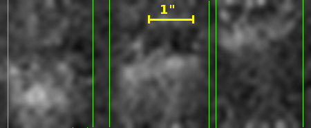
Figure 5.— The 2D GMOS spectrum of SGAS J105039.6$+$001730 is shown, zoomed in on the region where the C III] doublet appears and smoothed with a gaussian kernel with $\sigma=1$ detector pixel. The vertical axis here is the direction of dispersion, the horizontal axis is the spatial direction along the detector, and the vertical green lines indicate the approximate edges of the three N&S slitlets that are plotted in Figure 2 with the spatial scale is indicated by the yellow bar. The C III] emission feature appears in all three N&S slitlets, and is clearly extended along the length of each slitlet.

3.5. PSF Matched Photometry

Photometry of the giant arc is performed using custom IDL code that lets us construct apertures which follow the ridge-line of the arc. Images are convolved to a common point spread function (PSF) so that the apertures can be defined and applied to the same regions on the sky. This process is described in more detail in Wuyts et al. (2010) and Bayliss (2012). SGAS J105039.6$+$001730 has a total magnitude of F606W $=$ 21.48 $\pm$ 0.05 and $i=$ 21.18 $\pm$ 0.06.

3.6. Lensing Analysis

3.6.1 Strong Lens Model

In addition to SGAS J105039.6$+$001730, we identify several different strongly lensed background galaxies around the core of the foreground galaxy cluster; these are labeled in Figure 6. Galaxy A, at z $=$ 2.404, is lensed into a giant tangential arc (A1) and a radial arc (A2), both with similar morphology and colors in the HST and Spitzer data. Galaxy B is a faint tangential arc at unknown redshift. Galaxy D is lensed into four images (D1-4), spectroscopically confirmed to be at z $=$ 4.867 from Gemini/GMOS (D1) and Magellan/IMACS (D2,3,4).

Two images of galaxy C form the giant arc SGAS J105039.6$+$001730. One counter image (C3) at ($\alpha$,$\delta$) = 10:50:41.336, $+$00:17:23.35 (J2000) was spectroscopically confirmed by IMACS based on the presence of emission line features coincident with He II$\lambda$1640, C IV$\lambda$$\lambda$1448,1450 and C III]$\lambda$$\lambda$1907,1909 at the same redshift and in the same approximate relative strengths as observed in the GMOS spectrum of the main arc. Another image (C4) is predicted by the lens model and visually confirmed in the HST data, but lacks spectroscopic confirmation.

The positions and redshifts of the spectroscopically confirmed galaxies are used as constraints in the lens modeling process. With the exception of system C (SGAS J105039.6$+$001730), we use one position per image. For system C, we use the positions of the four brightest knots in C1 and C2, and the two brightest knots in C3.The lens model is computed using the publicly-available software, Lenstool (Jullo et al., 2007), utilizing a Markov Chain Monte Carlo minimizer both in the source plane and the image plane. The lens is represented by several pseudo-isothermal ellipsoidal mass distribution (PIEMD) halos, described by the following parameters: position $x$, $y$; a fiducial velocity dispersion $\sigma$; a core radius r_core; a cut radius r_cut; ellipticity $e=(a^{2}-b^{2}{)}/(a^{2}+b^{2})$, where $a$ and $b$ are the semi major and semi minor axes, respectively; and a position angle $\theta$. The PIEMD profile is formally the same as dual Pseudo Isothermal Elliptical Mass Distribution (dPIE, see Elíasdóttir et al., 2007).

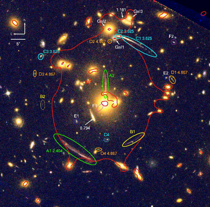
Figure 6.— Color composite image of the core of strong lensing cluster SDSS J1050+0017 using HST/WFC3 F160W,F110W,F606W. The critical curve of the best-fit lens model is plotted in red. Multiply-lensed galaxies are marked with ellipses, and their IDs and redshifts are labeled. The thick ellipses mark confirmed arcs, and thin ellipses mark arc candidates that were predicted by the lens model but not spectroscopically confirmed. The foreground galaxies that were individually modeled as contributing to the strong lensing are indicated. We also indicate other objects in the background of the clusters for which we measured spectroscopic redshifts. See $\S$ 3.6.1 for a complete description of the strong lens model.

Table 4Best-fit lens model parameters

Halo	RA	Dec	$e$	$\theta$	$r_{\rm core}$	$r_{\rm cut}$	$\sigma_{0}$
(PIEMD)	($\arcsec$)	($\arcsec$)		(deg)	(kpc)	(kpc)	(km s-1)
Cluster	$-0.73^{+0.21}_{-0.14}$	$3.07^{+0.61}_{-1.32}$	$0.10^{+0.04}_{-0.03}$	$72.6^{+10.5}_{-2.9}$	$81.2^{+12.0}_{-20.9}$	[1500]	$1029^{+32}_{-55}$
BCG	[0.0]	[0.0]	[0.067]	[-81.3]	[0.19]	[38.2]	$492^{+43}_{-48}$
Gal1	[3.37]	[22.33]	[0.0]	[0.0]	[0.08]	[27.1]	$124^{+18}_{-10}$
Gal2	[1.56]	[25.42]	[0.081]	[24.1]	[0.14]	[28.3]	$234^{+19}_{-17}$
Gal3	[8.37]	[29.13]	[0.083]	[71.2]	[0.09]	[17.1]	$177^{+40}_{-35}$
Fixed components
Halo2	[7.11]	[290]	[0.0]	[0.0]	[100]	[1500]	[950]
L* galaxy	$\cdots$	$\cdots$	$\cdots$	$\cdots$	[0.15]	[40]	[140]

Note. — All coordinates are measured in arcseconds relative to the center of the BCG, at [RA, Dec]=[162.66637 0.285224]. The ellipticity is expressed as $e=(a^{2}-b^{2})/(a^{2}+b^{2})$. $\theta$ is measured north of West. Error bars correspond to 1 $\sigma$ confidence level as inferred from the MCMC optimization. Values in square brackets are for parameters that were not optimized. The location and the ellipticity of the matter clumps associated with the cluster galaxies and the BCG were kept fixed according to their light distribution, and the fixed parameters determined through scaling relations (see text).

All the parameters of the cluster PIEMD halo were allowed to vary except for $r_{cut}$, which is not constrainable by the lensing evidence and was thus set to 1.5 Mpc. We selected cluster member galaxies in the $\sim 30^{\prime}$ SuprimeCam field of view, as red-sequence galaxies in a color-magnitude diagram. All galaxies within $6.5\arcmin$ from the BCG and brighter than $i=23$ mag were included in the model, with positional parameters ($x$, $y$, $e$, $\theta$) that follow their observed measurements, $r_{core}$ fixed at 0.15 pc, and $r_{cut}$ and $\sigma$ scaled with their luminosity (for a description of the scaling relations see Limousin et al., 2005). Four foreground galaxies have a more direct influence on the lensed galaxies due to their proximity to the lensed images. We thus allowed their velocity dispersions to be solved for in the lens modeling process. In particular, we note a galaxy at ($\alpha$,$\delta$) = 10:50:39.704, $+$00:17:29.14 – identified as “Gal1” in Figure 6 – that is not on the cluster red sequence, but its perturbation of the lensing potential is key to the lensing configuration of SGAS J105039.6$+$001730. Since the deflection is linear both with the distance term and the velocity dispersion, we included this galaxy in the same lens plane as the cluster, but note that its best-fit fiducial velocity dispersion scales with its dynamical mass and with its distance term. This approach is described in more detail by Johnson et al. (2014). We are ignoring the second order effects that result from halos residing in different lens planes (D’Aloisio et al., 2013; McCully et al., 2014), including other projected structure which exists along the line-of-sight toward the cluster lens, SDSS J1050+0017 (Bayliss et al., 2014), but these corrections contribute insignificantly to the uncertainty in the magnification derived from our lens modeling of this cluster.

The distribution of cluster galaxies shows a secondary concentration $\sim 290^{\prime\prime}$ north of the BCG. Thus another PIEMD halo is included at the position of the brightest galaxy at that position (see Table 4). The inclusion of that structure is also supported by the weak lensing analysis of Oguri et al. (2012).

The results of preliminary lens models indicated that several parameters are not well constrained by the lensing evidence. These include all the parameters of the secondary cluster-scale halo (a large range in $\sigma$ is allowed), and the scaling relation parameters for cluster member halos; these parameters were fixed in subsequent models. Table 4 lists the best-fit parameters and uncertainties, and values of fixed parameters. The model uncertainties were determined through the MCMC sampling of the parameter space and 1$\sigma$ limits are given. The image plane RMS of the best-fit lens model is $0\farcs 31$.

The lensing cluster SDSSJ 1050+0017 was first published by Oguri et al. (2012), which included a simplified strong lens model. The model was based on constraints from only one lensed galaxy (A), and assuming $z=2\pm 1$ as a best-guess for its redshift, which was not measured at the time. Oguri et al. (2012) report an Einstein radius for the fiducial arc redshift of 16.1″ with large error bars due to the redshift uncertainty. For the same arc, we find that the Einstein radius (defined here as the radius of a circle with the same area as the critical curve) is 17.5″, well in line with the initial model presented by Oguri et al. (2012).

3.6.2 The Magnification of SGAS J105039.6$+$001730

The lensing magnification depends strongly on the location along the arc. Areas in close proximity to the critical curve (plotted as a red line in Figure 6) have the highest magnification, and the magnification decreases farther from the critical curve. To convert the measurements in this paper to their intrinsic, unmagnified values, we calculate the total magnification inside the relevant aperture within which each measurement was made. The boundaries of the aperture are ray-traced to the source plane; we then measure the area covered by the aperture in the image plane, and divide it by the area covered by that aperture in the source plane, thus averaging over magnification gradients within the aperture. This approach overcomes the problem of pixels very close to the critical curve with extremely high magnification artificially driving the average magnification to a higher value.

To derive the uncertainties in the magnification, we compute many models with parameters drawn from the MCMC sampling which represent a 1$\sigma$ range in the parameter space. The total magnifications are $27.3^{+11.4}_{-6.5}$  in the aperture used for the FIRE spectroscopy, $31.9^{+10.7}_{-7.8}$  in the GMOS aperture, and $31.4^{+10.8}_{-3.5}$  in the aperture used for the photometric measurement of the arc.

We take the magnification factors that correspond to the slit apertures for the FIRE and GMOS spectrum to correct the line flux measurements described in $\S$ 3.1. The resulting magnification-corrected (i.e. intrinsic) emission line fluxes that result from the brightest knot (observed with FIRE, GMOS and MagE) are reported in Table 5.

Table 5Emission Line Flux Measurements

		measured flux	dereddened flux
Ion	$\lambda_{rest}$	$\times$10-18	$\times$10-18
		(erg cm-2 s-1)	(erg cm-2 s-1)
He II	1640.42	0.29$\pm$0.04	2.7${}^{+1.6}_{-1.1}$
O III]	1660.81	0.10$\pm$0.04	0.9${}^{+0.6}_{-0.4}$
O III]	1666.15	0.29$\pm$0.04	2.7${}^{+1.6}_{-1.1}$
N III]	1750.71	0.08$\pm$0.03	0.6${}^{+0.3}_{-0.2}$
Si III]	1882.47	0.26$\pm$0.04	2.1${}^{+1.1}_{-0.7}$
Si III]	1892.03	0.15$\pm$0.04	1.2${}^{+0.7}_{-0.4}$
C III]	1907.68	1.14$\pm$0.07	9.0${}^{+4.6}_{-3.0}$
C III]	1908.73	0.69$\pm$0.08	5.5${}^{+2.8}_{-1.9}$
O [II]	3727.09	2.26$\pm$0.06	8.6${}^{+2.6}_{-2.0}$
O [II]e	3729.88	2.22$\pm$0.06	8.4${}^{+2.6}_{-2.0}$
Ne [III]	3870.16	1.83$\pm$0.04	6.7${}^{+1.9}_{-1.6}$
H-$\gamma$	4341.68	2.96$\pm$0.12	9.5${}^{+2.5}_{-2.0}$
O [III]	4364.44	$<$0.81	$<$3.3
H-$\beta$	4862.68	5.71$\pm$0.06	16${}^{+4}_{-3}$
O [III]	4960.29	13.44$\pm$0.10	38${}^{+8}_{-7}$
O [III]	5008.24	46.12$\pm$0.12	127${}^{+29}_{-23}$

4. Recovering Physical Quantities

In this section we constrain various different physical properties of the lensed source, SGAS J105039.6$+$001730. The following subsections describe our methods for recovering parameter values, and the resulting values are shown in Table 6 (stellar mass, extinction, star formation rate, electron density & temperature, and ionization parameter) and Table 7 (metallicity and relative ionic abundances).

4.1. Broadband SED Fitting

We model the observed spectral energy distribution using the fitting code FAST (Kriek et al., 2009) at fixed spectroscopic redshift with Bruzual & Charlot (2003) stellar population synthesis models, a Chabrier (2003) IMF and Calzetti et al. (2000) dust extinction law. We adopt exponentially decreasing star formation histories with minimum e-folding time log($\tau$) $=$ 8.5 yrs (e.g., Wuyts et al., 2011) and the metallicity is allowed to vary from 0.2Z_⊙ to Z_⊙. This results in a stellar mass estimate log(M_∗/M_⊙) $=$ 11.0 $\pm$ 0.15 (statistical) $\pm$ 0.2 (systematic) M_⊙. We combine this with the magnification acting on the arc as computed from the strong lens models described above ($\mu=$ $31.4^{+10.8}_{-3.5}$) to recover the intrinsic stellar mass of SGAS J105039.6$+$001730: log(M_∗/M_⊙) $=$ 9.5 $\pm$ 0.15 (statistical) $\pm$ 0.2 (systematic)

Because of the relatively large point spread function (PSF) of the IRAC bands there is possible contamination in the measured flux of SGAS J105039.6$+$001730 in the IRAC 3.6 and 4.5$\mu$m bands from a nearby foreground galaxy that is separated from the arc by $\sim$1.5″. As a test we have explored SED fits with the IRAC flux reduced by a factor of 2$\times$ (an extreme case); we find that this factor of 2 contamination case only weakly affects the best-fit stellar mass, and that the possible contamination is sub-dominant to other systematic uncertainties in the SED-derived stellar mass (Shapley et al., 2005; Wuyts et al., 2011; Conroy et al., 2009, 2010; Conroy & Gunn, 2010).

4.2. Reddening Constraints from Balmer Lines

The H-$\beta$ and H-$\gamma$ Balmer lines are detected in the FIRE spectra, which allows us to place a constraint on the reddening due to interstellar dust in the rest-frame. H-$\beta$ is well-detected in the FIRE data, but unfortunately the H-$\gamma$ line falls in a region of poor atmospheric throughput and on top of sky lines, which degrades our ability to precisely measure the line flux. SGAS J105039.6$+$001730 appears from all indications to be a relatively low-mass galaxy with active ongoing star formation, so we assume a Calzetti et al. (2000) extinction law. The measured H-$\beta$/$\gamma$ ratio indicates an internal extinction of E(B-V) $=$ 0.14${}^{+0.38}_{-0.14}$, which is effectively an upper limit of E(B-V) $<$ 0.52. This agrees with the results of the best-fit SED model, which prefers A${}_{V}=$ 1.0 $\pm$ 0.2. From here on out we proceed with an extinction value of A${}_{V}=$ 1.0 and the Calzetti et al. (2000) extinction law and correct all reddening sensitive measurements accordingly. Achieving better constraints on the internal reddening will be challenging due to H-$\alpha$ being redshifted out of the K band, and H-$\gamma$ falling into a region of poor atmospheric transmission.

4.3. Damped Lyman-$\alpha$ Absorption

From the GMOS and MagE spectra it also appears as though SGAS J105039.6$+$001730 is a damped Lyman-$\alpha$ Absorption (DLA) system. The GMOS spectrum is higher S/N and we use it to fit a Voigt profile using the XIDL procedure x_fitdla. Even in the GMOS data the S/N is falling off rapidly in the region of the damped Ly-$\alpha$ absorption due to the combination of 1) the throughput of the grating decreasing at bluer wavelengths and 2) the continuum emission being suppressed by the Ly-$\alpha$ absorption. We use $\Delta\lambda\sim$5600-6200Å– corresponding to $\Delta\lambda\sim$1210-1340Å in the rest frame – to fit the DLA profile (see Figure 4). In this region of the spectrum the data fall off from S/N per spectral pixel of $\sim$6 at 6200Å to $<$1 at 5600Å. The low S/N limits our ability to precisely constrain the centroid of the DLA profile, but we find that the data prefer a high column density, log(N${}_{HI})>$ 21.5 cm^-2, independent of the precise redshift centroid of the DLA feature. The width of the velocity broadening component of the profile is also unconstrained. Higher S/N observations of the spectrum blueward of 6000Å will be necessary to make a precise measurement of the DLA feature, but the available data strongly indicate the presence of a large quantity of neutral hydrogen.

4.4. Star Formation Rate Estimates

Following the calibrations of Kennicutt (1998), we compute the star formation rate (SFR) from the FIRE observations of the brightest knot of SGAS J105039.6$+$001730  using the H-$\beta$ and [O II]$\lambda$$\lambda$3727,3729 emission lines. Both the H-$\beta$ and [O II]$\lambda$$\lambda$3727,3729 SFR estimates measure the instantaneous star formation, because they probe the integrated luminosity of massive stars blueward of the Lyman limit (i.e. ionizing photons). We correct these SFR measurements by using the strong lens model described in $\S$ 3.6.1 to compute the magnification factor that applies to the region of the arc covered by the FIRE slit. In this case, the FIRE slit measures a region of the arc with a total magnification, $\mu=$ $27.3^{+11.4}_{-6.5}$, and after correcting for this magnification we compute the SFR (for the knot covered by FIRE only) of SFR${}_{H\beta}=$ 84 $\pm$ 24 M_⊙ yr^-1 and SFR${}_{OII}=$ 55 $\pm$ 25 M_⊙ yr^-1, where the large uncertainties reflect a 20% uncertainties in the absolute flux calibration of the FIRE data, as well as measurement errors and a 30% scatter in the calibration between and luminosity in the case of SFR_OII.

4.5. Electron Density

Our spectra include three distinct doublet lines that provide a measurement of the electron density, n_e, in the HII regions that are responsible for the observed nebular line emission (Osterbrock, 1989). The GMOS spectrum contains both C III]$\lambda$$\lambda$1907,1909 and Si III]$\lambda$$\lambda$1882,1893, where the Si lines are well-separated and the C III] lines are blended but resolved. The FIRE spectrum resolves the [O II] $\lambda$$\lambda$3727,3729 lines. All of these line pairs are located very close to one another in wavelength so that the uncertainty regarding the internal reddening does not factor into the electron density determination. We use the curves from Osterbrock (1989) to convert line ratios into electron density; the reported uncertainties are those associated with the measurement uncertainties in the line ratios and assume no additional systematic uncertainties in the line ratio vs. n_e curves of Osterbrock (1989). We compute initial estimates of the electron density beginning with an assumed electron temperature, T${}_{e}=$ 10,000 K, and then iterate the computations described in this Section and the following section to arrive at the converged values presented here.

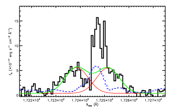
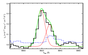
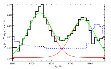
Figure 7.— Top: The double gaussian fit to the [O II] $\lambda$$\lambda$3727,3729 doublet. The FIRE spectrum is plotted as the black solid histogram, with the uncertainty plotted as the blue dashed histogram. Over-plotted in are the individual gaussian fits (red curves) to the two [O II] lines, along with the sum of the two gaussians (green curve). These lines are coincident with a bright sky line, which appears to have produced an artificial deficit of flux blueward of the centroid of the sky line and an excess redward. The double gaussian fit allows us to recover a good estimate of the true line shapes and strengths of the [O II] doublet. Middle: The double gaussian fit to the C III]$\lambda$$\lambda$1907/1909 doublet. Again, the GMOS spectrum is plotted in black with the uncertainty in blue (and dashed). Individual (red curves) gaussians for the separate lines, as well as the summed double gaussian profile (green curve) are over-plotted. Bottom: The double gaussian fit to the Si III]$\lambda$$\lambda$1882,1892 doublet using the same line/color scheme as the middle panel. The Si small III lines are well-separated in our spectra (though the lines have much lower S/N than the [O II] and C III] doublets).

The cleanest lines that we can measure in the available data are Si III]$\lambda$$\lambda$1882,1892, which are well-separated in wavelength and unaffected by strong sky subtraction residuals. We also measure the line ratios for C III] and [O II], though systematic uncertainties from sky lines make them both less robust measurements than the Si III] ratio. The C III] and Si III] lines both probe a relatively higher density range and therefore cannot precisely constrain n_e values below $\sim$ 10³ cm^-2; the [O II]$\lambda$$\lambda$3727,2729 line ratio provides constraints below n${}_{e}\sim$ 10³ cm^-2 but are unfortunately limited by a bright sky line residual in our data. The specific n_e constraints from are data are summarized as follows:

1. Si III]$\lambda$$\lambda$1882,1892 — We measure this line ratio to be 1.6 $\pm$ 0.2 in the GMOS spectrum. This value corresponds to an electron density n${}_{e}=$ 10³ cm^-2 for nebular line emitting regions within SGAS J105039.6$+$001730. Incorporating the uncertainty in the Si III] line ratio results in an upper limit, n${}_{e}\leq$ 2 $\times$ 10³ cm^-2. This is fully consistent with SGAS J105039.6$+$001730 being in the low-density regime, though the Si III] doublet ratio transitions at higher densities and therefore does not provide as powerful a constraint on low density values of n_e as as well-measured [O II] 3727,2729 line ratio would.

2. [O II]$\lambda$$\lambda$3727,2729 — The measurement of [O II]$\lambda$$\lambda$3727,3729 is complicated by the unfortunate fact that the lines are redshifted onto the location of a bright sky line in the NIR. In order to attempt to recover the line ratio from the FIRE data we fit a double gaussian profile to the resolved [O II]$\lambda$$\lambda$3727,3729 lines, holding the redshift fixed to the values taken from the mean of the other nebular emission lines apparent in the FIRE data (see Table 3). This line profile fitting method allows us to recover an estimate of the true line strengths, ignoring contamination from the bright sky line residuals. We measure a line ratio of 1.0 $\pm$ 0.4; the central value implies an electron density of n${}_{e}\sim$ 2-3$\times$10² cm^-2, though the large uncertainty effectively encompasses all physically plausible density values.

3. C III]$\lambda$$\lambda$1907,1909 — The C III]$\lambda$$\lambda$1907,1909 line ratio is fit in the same way as the [O II]$\lambda$$\lambda$3727,3729, and we find a line ratio of 1.65 $\pm$ 0.14, which is non-physical but less than 1$\sigma$ from the maximum value for the line ratio in the low-density limit ($\sim$1.55), and implies a 2$\sigma$ limit of n${}_{e}\lesssim$ 3$\times$10³ cm^-2. We also note that the line measurements for C III] suffer from a similar source of uncertainty as the O II]$\lambda$$\lambda$3727,2729 doublet due to the lines being redshifted to fall on to a bright sky line. However the nod-and-shuffle strategy employed with the GMOS data helps significantly in limiting the sky line subtraction uncertainties to the poisson minimum.

The two gaussian profile fits to each of the [O II], C III], and Si III] doublets are shown in Figure 7. From the three electron density indicators, there is a strong preference for the low-density regime, with n${}_{e}\leq$10³ cm^-2. We also note that the apparent offset in density values preferred by the [O II] and C III] doublets may simply reflect the fact that these doublets trace the electron density of the low and medium ionization zones, respectively (Quider et al., 2009; Christensen et al., 2012a; James et al., 2014).

4.6. Electron Temperature

There is very strong [O III]$\lambda$$\lambda$4960,5008 emission, but no detection of [O III]$\lambda$4364 in the FIRE spectrum. We use the non-detection of [O III]$\lambda$4364 to place a limit on the electron temperature in the nebular line emitting regions following the method of Izotov et al. (2006) (Section 3.1, Equations 2 & 3). Izotov et al. (2006) point out that the electron density becomes unimportant to the electron temperature determination for values of n${}_{e}\lesssim 10^{3}$ cm^-2, and our constraint on n_e from the previous section places SGAS J105039.6$+$001730 in that regime. From the [O III]$\lambda$$\lambda$4960,5008 lines and the [O III]$\lambda$4364 limit we place a limit on T_e (O III) $\leq$ 14,000 K.

An alternative method for estimating the electron temperature is available to us by measuring the flux ratios between the O III]$\lambda$$\lambda$1661,1666 and [O III]$\lambda$$\lambda$4960,5008 (Villar-Martín et al., 2004; Erb et al., 2010). We have good detections of all the relevant lines, so this method allows us to measure a precise temperature rather than a limit. However, this measurement has its own caveats, primarily a large sensitivity to the intrinsic extinction, and a large uncertainty between the absolute flux calibrations of the optical (GMOS) and NIR (FIRE) spectra. With these caveats in mind, we measure T_e = 11300${}^{+1400}_{-1000}$ K (measurement uncertainties only), which agrees well with the T_e constraint from the FIRE spectrum alone. When we fold in the additional uncertainty between the relative flux calibrations of the GMOS and FIRE data, as well as the uncertainty in our best-fit value for the dust extinction (A${}_{V}=1\pm 0.2$) we find that T_e constraint from the O III]$\lambda$$\lambda$1661,1666 to [O III]$\lambda$$\lambda$4960,5008 line ratio is quite broad: 4000 $<$ T_e $<$ 15000 K. This is less constraining (for physically plausible values of T_e) than the limit derived from the non-detection of [O III]$\lambda$4364. From here on out we proceed with the T_e $\leq$ 1.4 $\times$ 10⁴ K constraint on the electron temperature.

Table 6Physical Parameter Constraints

Physical	Value
Quantity
log(M∗/M⊙)	9.5 $\pm$ 0.35
AV	1.0 $\pm$ 0.2
NHI (cm-2)	$\geq$ 1021.5
SFRHβ (M⊙ yr-1)	84 $\pm$ 24
SFROII (M⊙ yr-1)	55 $\pm$ 25
ne (cm-3)	$\leq$ 103
Te ($\lambda$4364) (K)	$<$ 14000
Te ($\lambda$$\lambda$1666) (K)	$<$ 15000
log(U) (O3O2)	$-$2.22 $\pm$ 0.15
log(U) (Ne3O2)	$-$2.7${}^{+0.3}_{-0.2}$

4.7. Oxygen Abundance Indicators

In the the next two subsections we apply several different Oxygen and ionic abundance indicators to our observations of SGAS J105039.6$+$001730. The results are summarized in Table 7. For all of these calculations we include a systematic uncertainty term that results from the uncertainty in the extinction correction (A${}_{V}=1\pm 0.2$) that is applied to the Oxygen lines.

4.7.1 T_e Direct Oxygen Metallicity

From the detected oxygen lines we can use the direct T_e method to constrain the metallicity of SGAS J105039.6$+$001730 using the prescription outlined by Izotov et al. (2006). This metallicity measurement accounts for the singly (O⁺/H⁺) and doubly ionized (O⁺⁺/H⁺) oxygen atoms, but ignores triply ionized oxygen which only contributes significantly to the measured abundance in regions of extremely high ionization. The metallicity constraint from this method is 12 $+$ log(O/H)${}_{Te}\geq$ 8.05 ($\geq$ 0.22Z_⊙) when we use the upper limit on the electron temperature from the [O III]$\lambda$$\lambda$4960,5008 to [O III]$\lambda$4364 ratio.

4.7.2 R₂₃

The R₂₃ index measures the strength of [O II] and [O III] lines against Balmer line emission from hydrogen: log([$\lambda$3727$+\lambda$3729$+\lambda$4960$+\lambda$5008]/H-$\beta$). This index is problematic because it is double valued, with both high metallicity and low metallicity branches. We measure log(R₂₃) $=$ 1.05 $\pm$ 0.06. The high value for R₂₃ places SGAS J105039.6$+$001730 in the transition zone between the upper and lower branches of the observed R₂₃ – metallicity relation. There are several different calibrations for the R₂₃ index in the literature for one or both branches; we compute the R₂₃ based 12 $+$ log(O/H) for these different calibrations.

The upper branch calibration of Zaritsky et al. (1994) yields 12 $+$ log(O/H)${}_{ZKH94}=$ 8.30 $\pm$ 0.09, or 0.4Z_⊙, in good agreement with both the limit and the measurement from the T_e method. Using the calibration of Pilyugin & Thuan (2005) we get an upper branch abundance of 12 $+$ log(O/H)${}_{P05,upp}=$ 8.19 $\pm$ 0.11 and a lower branch value of 12 $+$ log(O/H)${}_{P05,low}=$ 8.16 $\pm$ 0.11. Finally, we also apply the R₂₃ calibration of Kobulnicky & Kewley (2004), which yields an upper branch value of 12 $+$ log(O/H)${}_{KK04,upp}=$ 8.49 $\pm$ 0.11 and a lower branch value of 12 $+$ log(O/H)${}_{KK04,low}=$ 8.26 $\pm$ 0.11.

4.7.3 Ne3O2

The ratio of [Ne III]$\lambda$3869 to [O II]$\lambda$$\lambda$3727,3729 has also been calibrated as an indicator of the log(O/H) metallicity by Shi et al. (2007). We measure log(3869/3727$+$3729) $=$ $-$0.41, which corresponds to 12 $+$ log(O/H) $=$ 7.5 $\pm$ 0.2. The error bar reported here does not include the uncertainty in the zero point of the Ne3O2 calibration, which is quite large ($\sim$ 0.7 dex), and while we report the Ne3O2 metallicity estimate in the spirit of being thorough, we do not use it to compute the mean metallicity of SGAS J105039.6$+$001730 (see Table 7).

4.7.4 Average Oxygen Abundance Metallicity

In addition to the results of each of the individual Oxygen abundance metallicity indicators, we also show in Table 7 the average metallicity value of all of the Oxygen abundance indicators calculated in the previous sections, excluding the Ne3O2 method due to the extremely large uncertainty in the zero point of the Ne3O2 metallicity diagnostic.

4.8. Ionic Abundance Ratios

4.8.1 Ionization Parameter, log(U)

From the available data we can follow Kewley & Dopita (2002) and Kobulnicky & Kewley (2004) to estimate the ionization parameter from the ratio of [O III] to [O II] line fluxes. This is computed iteratively with the Kobulnicky & Kewley (2004) oxygen abundance computed in $\S$ 4.7, above. The preferred ionization parameter from the rest-frame optical emission lines is log(U) $=$ $-$2.22 $\pm$ 0.15. This ionization parameter is not nearly so extreme as has been found in a few extreme star bursting galaxies at z $\sim$2-3.3, where log(U) is measured to be as high as $\sim-1$ (e.g.; Villar-Martín et al., 2004; Erb et al., 2010). We also use the Ne3O2 line ratio diagnostic for recovering the ionization parameter as recently proposed by Levesque & Richardson (2014), which we agree is likely a much better use of this line ratio measurement than the Ne3O2 metallicity indicator. Ne3O2 yields an ionization parameter estimate of log(U) $=$ $-$2.7${}^{+0.3}_{-0.2}$. The uncertainty here includes contributions from the line flux measurements, the reddening correction, and the $\sim 0.1$dex uncertainty in the average metallicity measurement (see Table 7).

It is not clear which of the two diagnostics above provides the more reliable estimate of log(U). There are reasons to suspect, however, that both of the preceding ionization parameter estimates are unreliable, or at least incomplete in their description of the physical conditions within SGAS J105039.6$+$001730. Specifically, the detection of strong He II$\lambda$1640 emission, and significant excess emission in the P Cygni line profiles of Si IV and C IV both prefer larger values of log(U). We discuss these features in more detail in $\S$ 4.10 and $\S$ 5.3.

Table 7Ioni Abundance Measurements

Ion Abundance Ratio	Value
12 $+$ log(O/H) (Te Direct)……………………	$>$8.05
12 $+$ log(O/H) (R23,ZKH94)…………………	8.30 $\pm$ 0.09
12 $+$ log(O/H) (R23,P05-upp)……………….	8.19 $\pm$ 0.11
12 $+$ log(O/H) (R23,P05-low)……………….	8.16 $\pm$ 0.11
12 $+$ log(O/H) (R23,KK05-upp)…………….	8.49 $\pm$ 0.10
12 $+$ log(O/H) (R23,KK05-low)…………….	8.26 $\pm$ 0.10
12 $+$ log(O/H) (Ne3O2)……………………….	7.5 $\pm$ 0.2 ($\pm$ 0.7)
$<$12 $+$ log(O/H)$>$ (excl. Ne3O3)………….	8.28 $\pm$ 0.13
$<$Z/Z⊙$>$…………………………………………….	0.39${}^{+0.13}_{-0.10}$
12$+$log(Ne++/H+) (Ne++/H+)…………….	7.13 $\pm$ 0.23
log(C++/O++) ($\lambda$1909/$\lambda$1666)……………..	$-$0.79 $\pm$ 0.06
log(C++/O++) ($\lambda$1909/$\lambda$5008)……………..	$-$0.77$\pm$ 0.32
log(N++/O++) ($\lambda$1750/$\lambda$1666)……………..	$-$1.2 $\pm$ 0.3
log(Si++/C++) ($\lambda$1892/$\lambda$1909)……………..	$-$1.2 $\pm$ 0.3
log(Si++/O++) ($\lambda$1892/$\lambda$1666)……………..	$-$2.0 $\pm$ 0.4

4.8.2 Ne⁺⁺ Abundance

From the strong [Ne III]$\lambda$3869 emission line we can compute the abundance of Ne⁺⁺/H⁺ using equation 7 from Izotov et al. (2006). We find 12 $+$ log(Ne⁺⁺/H⁺) $=$ 7.13 $\pm$ 0.23. In the Lynx arc, Villar-Martín et al. (2004) approximate that all of the nebular Ne atoms are doubly ionized, so that Ne/H $\sim$ Ne⁺⁺/H⁺, but it’s not clear that we can make the same assumption given that we measure an [O II] to [O III] ratio that is consistent with an ionization parameter that is considerably lower than the log(U) $\sim$ $-$1 that is found in the Lynx arc. We can at least note the lack of observable flux from known Ne IV and Ne V lines in both the rest-UV and rest-optical, which qualitatively argues against these states representing a large fraction of the total Ne.

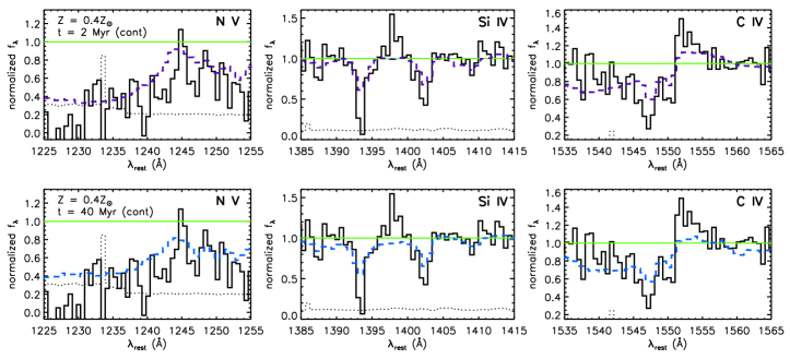
Figure 8.— Comparison of continuous star formation S99 models against the P Cygni features in the GMOS spectrum. The GMOS data are plotted as solid histograms, with the error array over plotted as a dotted line and the fiducial continuum level indicated by the horizontal green line. The S99 models based on empirical LMC/SMC stellar atmospheres are over plotted as the color dashed lines. Each row is a different S99 model: the ages of the stellar populations are varied between the top and bottom rows.

4.8.3 C⁺⁺/O⁺⁺ Abundance Ratio

Garnett et al. (1995b) used HST spectroscopy of dwarf galaxies to measure the relative abundances of C⁺⁺/O⁺⁺ and N⁺⁺/O⁺⁺ from rest-UV emission lines. We detect the same families of lines in the GMOS spectrum of SGAS J105039.6$+$001730 and can therefore measure the ion abundance ratios of this galaxy at z $=$ 3.6252. We use the ratio of the line intensities of O III]$\lambda$$\lambda$1661,1666 and C III]$\lambda$$\lambda$1907,1909 (Garnett et al., 1995b) to measure log(C⁺⁺/O⁺⁺) $=$ $-$0.79 $\pm$ 0.06. This abundance measurement is relatively insensitive to extinction due to the similar wavelengths of the lines.

Kobulnicky & Skillman (1998) have also shown that it is possible to measure the C⁺⁺/O⁺⁺ from the relative line strengths of C III]$\lambda$$\lambda$1907,1909 and [O III]$\lambda$$\lambda$4960,5008. From this method we measure log(C⁺⁺/O⁺⁺) $=$ $-$0.77 $\pm$ 0.32, where the larger uncertainty is driven by the uncertainty in the reddening correction due to the fact that the lines used with this method span a large range in wavelength. Comparing the two C⁺⁺/O⁺⁺ measurements we see remarkable agreement, which could be interpreted as a confirmation that A${}_{V}=1$ is, in fact, an appropriate extinction value for SGAS J105039.6$+$001730. However, the values reported here do not reflect the uncertainty that results from the lack of a precise electron temperature constraint, and it is possible that the agreement results in part from different sources of error fortuitously canceling out.

Previous investigations have shown that there is no appreciable ionization correction factor (ICF) necessary for comparing C/O ion ratio given log(U) values in line with what we find above for SGAS J105039.6$+$001730 (Garnett et al., 1995b; Erb et al., 2010). If our estimate of log(U) is correct then the log(C⁺⁺/O⁺⁺) measurements above are effectively telling us the total log(C/O) elemental abundance ratios in SGAS J105039.6$+$001730.

4.8.4 N⁺⁺/O⁺⁺ Abundance Ratio

Similar to the C/O ratio measurement, Garnett et al. (1995b) use the ratio of the O III]$\lambda$$\lambda$1661,1666 lines and the N III]$\lambda$1750 multiplet to measure the N/O abundance. Nitrogen has ionization potentials that are closer to oxygen than carbon, and so an ionization correction factor should also not be necessary for inferring the total N/O ratio using the N⁺⁺/C⁺⁺ ion ratio. Applying this method we measure log(N⁺⁺/O⁺⁺) $=$ $-$1.6 $\pm$ 0.2, which assuming a negligible ICF, provides an estimate of the relative C/N enrichment: log(C/N) $=$ 0.8 $\pm$ 0.2.

4.8.5 Si⁺⁺/C⁺⁺ and Si⁺⁺/O⁺⁺ Abundance Ratios

Garnett et al. (1995a) demonstrate how the Si/O relative abundance can be computed from the rest-UV Si III]$\lambda$$\lambda$1882,1892 and C III]$\lambda$$\lambda$1907,1909 lines. As shown by Garnett et al. (1995a), the ICF for using the ratio of Si⁺⁺ to C⁺⁺ as an approximation of the total Si/C abundance is somewhat sensitive to the ionization parameter. Our estimate of log(U) for SGAS J105039.6$+$001730 implies a fraction of doubly ionized oxygen of X(O⁺⁺) $\sim$ 0.8-0.85 based on the models from Erb et al. (2010). From Garnett et al. (1995a) this implies X(Si⁺⁺)X(C⁺⁺) $\sim$0.65-0.9. This abundance estimate has a 25% uncertainty from the ICF alone; we estimate it to be in the range $\sim$1.1-1.5 with a central value of 1.4 (see, e.g.; Kobulnicky & Skillman, 1998). We find log(Si⁺⁺/C⁺⁺) $=$ $-$1.2 $\pm$ 0.3. Assuming our assumptions about the ICF are reasonable, this measurement can be combined with our measurements of the log(C/O) abundances to yield log(Si⁺⁺/O⁺⁺) $=$ $-$2.0 $\pm$ 0.4.

4.9. Starburst99 Model Comparisons

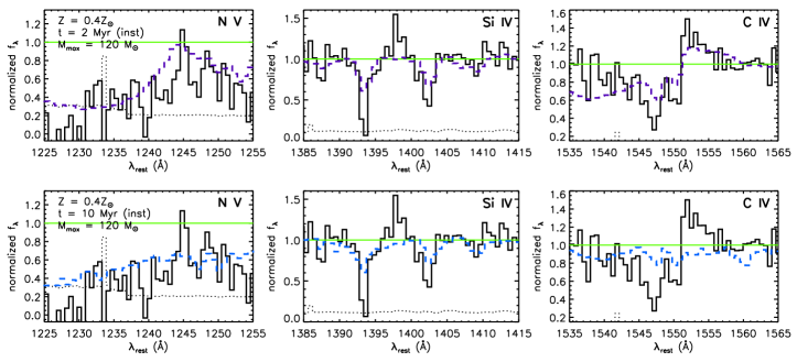
Figure 9.— S99 models created assuming a single instantaneous burst of star formation rather than the continuous star formation models. The panels are similar to those plotted in Figure 8, with the top and bottom rows showing stellar populations of two different ages. These models allow for stars up to 120M_⊙ to form, which results in strong C IV emission at early times (see the top row of panels) but still does not reproduce the combination of absorption and emission P Cygni features that we observe in SGAS J105039.6$+$001730.

The P Cygni ISM absorption/emission features that we observe in the rest-UV are the byproduct of powerful winds that are typically associated with Wolf-Rayet (W-R) stars. To try and understand the physical implications of the wind features in the spectrum of SGAS J105039.6$+$001730, we compare our data against Starburst99 models (S99; Leitherer et al., 2010).

Both our GMOS and MagE data include each of the N V$\lambda$$\lambda$1238,1240, Si IV $\lambda$$\lambda$1393,1402, and C IV$\lambda$$\lambda$1548,1551 doublets, though the N V$\lambda$$\lambda$1238,1240 feature is never detected at high S/N. The MagE spectrum is much higher spectral resolution than the GMOS spectrum, and would be the ideal dataset for comparison against synthetic spectra. However, we were limited to collecting 1 hr of integration time with MagE, and that taken at relatively high airmass and in highly variable seeing. As a result, the MagE data do not provide a superior comparison against the S99 model spectra than the GMOS data, and so we focus on S99 model-GMOS comparisons from here on out.

We generate an array of S99 models assuming both continuous and instantaneous star formation scenarios. The continuous star formation models also spanning a range in metallicities from from solar to 2% solar, and a range in ages of 2 Myr to 40 Myr. Our instantaneous models all assume a metallicity of 0.4Z_⊙ and span the range in ages (2–100 Myr), and also allow for variation in the maximum stellar mass formed, ranging from 30–120 M_⊙. In Figure 8 we plot two of the continuous star formation model synthetic spectra on top of the GMOS data in the regions surrounding the three strong P Cygni features noted previously (N V, S IV and C IV). The specific models plotted have metallicities of 0.4Z_⊙ – in line with the metallicity we measure from nebular line diagnostics – and ages of 2 Myr and 40 Myr. The S99 synthetic spectra assuming an instantaneous burst of star formation are shown in Figure 9, also plotted for two stellar population ages (2 Myr and 10 Myr). None of the models with either continuous or instantaneous star formation can reproduce the combination of narrow and deep absorption features, the shape of the absorption trailing off blueward of the C IV line center, or the narrow and strong emission from Si IV and the broader strong emission from C IV. The strength of the observed Si IV and C IV emission could imply that these features are at least partly nebular in origin, rather than resulting entirely from the winds and atmospheres of massive stars.

4.10. He II Emission

He II $\lambda$1640 emission appears in the GMOS and MagE spectra of SGAS J105039.6$+$001730. This feature appears in composite spectra of z $\sim$ 3 galaxies (Shapley et al., 2003) and in the spectrum of individual strongly lensed z $\sim$ 2-4 galaxies (e.g.; Cabanac et al., 2008; Dessauges-Zavadsky et al., 2011), but typically appears as a broad emission feature that is associated with the winds of W-R stars, and exhibits velocity widths of $\sim$1000 km s^-1. However, the He II $\lambda$1640 detected from SGAS J105039.6$+$001730 has a width of $\sim$330 km s^-1 in the GMOS spectrum, which matches the resolution of that data. The feature is too low S/N in the MagE spectrum to inform a multiple component fit to the velocity profile, but a simple gaussian fit to the line prefers a FWHM that is consistent with the resolution of the MagE spectra ($\sim$75 km s^-1), implying that a significant fraction of the emission does indeed originate from a narrow distribution in velocity space, and therefore is likely resulting from nebular emission rather than W-R winds.

Explaining such strong, narrow emission from He II requires extreme ionization. The He II$\lambda$1640 line is extremely bright in SGAS J105039.6$+$001730, with a total flux ratio of He II $\lambda$1640/H$\beta$ $\sim$ 0.17 after applying the extinction correction, and likely originates in part from nebular emission. Erb et al. (2010) note the presence of significant nebular HeII $\lambda$1640 emission in a bright field-selected LBG at z $=$ 2.3, and find that high ionization parameter values are required to explain the ratio that they measure for He II $\lambda$1640/H$\beta$ of 0.3, and an equivalent width of 2.7Å.

We can also compare the equivalent width, W₁₆₄₀, of He II $\lambda$1640 in SGAS J105039.6$+$001730 against predictions for the Wolf-Rayet wind He II $\lambda$1640 emission strength in the S99 models described above; we measure W${}_{1640}=$ 1.5 $\pm$ 0.15 Å. The S99 models only generate values this high for an extremely short-lived stretch (t${}_{age}\sim$ 5–7 Myr) and only in models with solar metallicity (in strong disagreement with all of the metallicity diagnostics measured in $\S$ 4.7). And as noted previously, He II $\lambda$1640 emission originating from W-R winds would be much broader than the unresolved line that we see in the GMOS spectrum. Lastly, we also see no evidence of a P Cygni blue shifted absorption feature in the He II $\lambda$1640 feature, which further argues against this line as originating entirely from W-R winds.

5. Discussion

5.1. Morphology of SGAS J105039.6$+$001730

HST imaging enables us to examine the morphology of SGAS J105039.6$+$001730 via both the internal structure of the arc itself, as well as the much less distorted counter image. The counter image appears extremely irregular, and contains several distinct emission knots. The giant arc also includes multiple images of three distinct knots of emission, one of which is considerably redder than the rest of the arc. The central emission knot in the counter image also appears notably redder. While the knots have different IR-optical colors, all are extremely bright in the optical (rest-UV). This suggests that there is active star formation throughout SGAS J105039.6$+$001730, but that the redder central knot likely has a a larger underlying population of older stars. It is possible that the redder knot corresponds to the core of the galaxy, which possibly hosts the early stages of an assembling bulge, and that the bluer emission from the outskirts of the galaxy is preferentially tracing small but intense star forming regions.

5.2. Comparison Against Low Redshift Galaxies

5.2.1 Strength of the C III] Feature

Strong C III]$\lambda$$\lambda$1907,1909 emission is not ubiquitous in star forming galaxies at moderate redshift (e.g., z $\sim$ 2 composite; Shapley et al., 2003). It is therefore interesting to compare SGAS J105039.6$+$001730 against individual low redshift star forming galaxies with good UV spectra to try and understand the astrophysical conditions that are conducive to producing strong C III]$\lambda$$\lambda$1907,1909. The galaxy sample compiled by Leitherer et al. (2011) (hereafter L11) is an excellent comparison set, with HST UV spectra of 46 star forming regions within 28 galaxies with z $<$ 0.06.

We examine the individual spectra that were analyzed in L11, and measure the equivalent width, W₁₉₀₉, of the C III]$\lambda$$\lambda$1907,1909 line in the L11 spectra. In Figure 10 we show the relationship between W₁₉₀₉ and metallicity in the L11 sample; there is a dearth of galaxies with both a large W₁₉₀₉ and high metallicity, indicating that C III]$\lambda$$\lambda$1907,1909 emission may be suppressed in high metallicity star forming galaxies. Interestingly, SGAS J105039.6$+$001730 has a larger W₁₉₀₉ than all but 2 of the 25 L11 galaxies, yet it has a metallicity, 12 $+$ log(O/H) $=$ 8.3, which coincides almost exactly with the apparent turn-off of strong C III] emission in the L11 sample. The C III] lines are forbidden and semi-forbidden transitions, so any such suppression must be the result of one or more indirect mechanisms, unlike the suppression of resonant lines such as Lyman-$\alpha$.

A similar relationship has also recently been observed in low-mass high redshift galaxies (Private communication; Stark et al. in prep, 2014), where W₁₉₀₉ appears to be correlated with the strength of Lyman-$\alpha$ emission. In this context SGAS J105039.6$+$001730 is puzzling, in that is exhibits a strong DLA feature, which is opposite of what one should expect given a correlation between W₁₉₀₉ and W_Ly-α. The strength of C III] emission in SGAS J105039.6$+$001730 is difficult to understand in light of this galaxy’s other observable properties and the apparent tendency for strong C III] emission to coincide with strong Ly-$\alpha$ emission and low metallicity. It would seem that the physics which dictate strong C III] cannot be summarized according to a simple correlation against a singe fundamental physical quantity (e.g., metallicity).

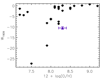
Figure 10.— Black notched diamonds show the equivalent width of the C III]$\lambda$$\lambda$1907,1909 doublet and metallicity for 25 galaxies in Leitherer et al. (2011) where the line is included in the spectral coverage of the available data and there is a metallicity measurement available. The same values for SGAS J105039.6$+$001730 are indicated by the solid purple triangle.

5.2.2 Relative C/O, N/O, Si/O Enrichment

With measurements of the relative abundance of C/O, N/O and Si/O we can compare the enrichment of the ISM in SGAS J105039.6$+$001730 against well-studied star forming galaxies at low redshift. Garnett et al. (1995b) examine the relative C/O, C/N and N/O abundances of irregular/HII galaxies at low redshift. SGAS J105039.6$+$001730 fits nicely onto the sequence of C/O vs. 12 $+$ log(O/H)  and C/N vs. 12 $+$ log(O/H) that Garnett et al. (1995b) observe.

The relative abundances of Si and O were also studied by Garnett et al. (1995a). Si and O should be produced in the same stars, and therefore their ratio is not expected to vary strongly with metallicity. Variations can occur, however, if Si depletes onto dust grains in the ISM, rendering it unobservable via observation of line emission from ionized HII regions. Our measurement of the Si/O abundance in SGAS J105039.6$+$001730  is somewhat lower than the stable value observed by Garnett et al. (1995a), but the large uncertainties prevent us from making a strong statement about whether or not Si depletion by the formation of silicate dust grains may truly be taking place in SGAS J105039.6$+$001730.

Our abundance measurements indicate that SGAS J105039.6$+$001730 has elemental enrichment properties that are generally in-line with observations of irregular star forming galaxies at z $\sim$ 0.

5.3. P Cygni Features

Based on the strength of the P Cygni features in SGAS J105039.6$+$001730, we expect the extremely low metallicity models to do a poor job of reproducing the observed features, and this holds true. Models with metallicities of 0.4Z_⊙ result in the best agreement with our data, which is encouraging given that we measure the metallicity to be $\sim$0.4Z_⊙ from nebular emission line diagnostics. However, none of the synthetic spectra that we generate using S99 produce the combination of P Cygni features that we observe in of SGAS J105039.6$+$001730. The most challenging features to explain are the narrow shape and exceptional strength of the blueshifted absorption features, as well as the strength of the redshifted C IV emission and the odd, strong emission from S IV$\lambda$1393. Qualitatively these features indicate the presence of an extremely young population of massive stars. Some recent work has also explored the ways in which stellar rotation can affect the spectra of massive stars, and find that including rotation effects in the modeling of stellar spectra can result in a increase in the amount of ionizing radiation, hardening of the ionizing radiation, and stronger profiles for some lines, including the UV Si IV and C IV P Cygni features (Levesque et al., 2012; Leitherer et al., 2014).

Our results here are reminiscent of the difficulty that other studies have encountered comparing synthetic spectra against observations of galaxies at z $\gtrsim$ 2 (Pettini et al., 2000; Shapley et al., 2003; Quider et al., 2009; Erb et al., 2010). As suggested by Erb et al. (2010), the excess emission features could be explained, at least in part, by nebular emission. The presence of nebular emission from these transitions does, however, agree with the properties of the He II$\lambda$1640 emission line discussed above, and would imply an extremely hard ionizing radiation field from massive O stars.

One possible explanation for what we observe in SGAS J105039.6$+$001730 is that the integrated spectrum that we measure across a wide range of wavelengths is a blend of the properties from several different star forming regions embedded within the galaxy. Different star forming regions could be generating extreme spectral features that dominate the observable signal in some regions of the spectrum (e.g., the rest-UV) while only contributing in part to other parts of the spectrum (e.g., the rest optical). The superposition of a “normal” star forming galaxy with small, highly magnified regions of intense and short-lived star formation could be responsible for generating the complex spectral features that defy reproduction by a simple monolithic synthetic population of stars. There is, in fact, a body of published work that uses real (Kobulnicky et al., 1999; James et al., 2013a, b) and simulated (Pilyugin et al., 2012) observations of well-studied low-redshift star forming galaxies to explore the biases that can result from simple analyses of the integrated spectra of distant galaxies. Recent observations of different line of sight within a single lensed star forming galaxy also shows clear evidence of different physical conditions in different star forming regions (Rigby et al., 2014). There is clear evidence to suggest that spatially resolved spectroscopy will be essential for constraining some of the physical properties of high redshift star forming galaxies.

5.4. Interpreting High Ionization Features in the Rest-UV

It is physically unlikely that all of our measured He II$\lambda$1640 line flux is nebular in origin, as that would require ionization parameters $>-1$ according to the models explored by Erb et al. (2010). Even assigning only $\sim$25% of the flux to nebular emission requires an ionization parameter, log(U) $>$ $-$2 for metallicities in the range that we measure for SGAS J105039.6$+$001730, according to the models explored by Erb et al. (2010). A physical picture in which there are one or more extreme star forming region(s) within SGAS J105039.6$+$001730 is also consistent with evidence that unresolved starbursts have a maximum ionization parameter, log(U) $\sim$ $-$2.3 (Yeh & Matzner, 2012), implying that diagnostics indicating significantly larger values of log(U) are likely to be sampling individual extreme star forming regions within galaxies (e.g., Snijders et al., 2007; Indebetouw et al., 2009).

Another possible explanation for the strong He II$\lambda$1640 line is the presence of an exceptionally hard ionizing spectrum. The ionization parameter, $U$, only describes the intensity of ionizing radiation; a very hard ionizing spectrum with relatively low intensity can generate a large amount of nebular He II emission even given a low ionization parameter. An initial mass function (IMF) that generates more of the hottest, most massive stars, for example, could account for a harder ionizing spectrum than considered by the models of Erb et al. (2010). However, arguments that are based on the vague, qualitative implications of varying the IMF are distasteful and presumptive when one considers that the spectral properties of the most massive stars are not well understood, especially at low metallicity (e.g., Rigby & Rieke, 2004).

The strong, narrow, He II $\lambda$1640 emission that we detect in SGAS J105039.6$+$001730 presents a puzzle. It either casts serious doubt on the ionization parameter diagnostics that we compute and rely on throughout $\S$ 4.8, or it suggests a hard ionizing spectrum that is difficult to reconcile with the electron temperature constraints available from rest-frame optical emission lines.

Returning to the explanation that we put forth in the previous subsection, it seems likely that the integrated spectrum of SGAS J105039.6$+$001730 is too complex to be described by a simple stellar population, or a single list of parameters (i.e., a single ionization parameter, electron temperature, metallicity, etc). Rather, it is possible that the [O III]$\lambda$$\lambda$4960,5008, [O II]$\lambda$$\lambda$3727,3729, [Ne III]$\lambda$3869, and He II $\lambda$1640 lines are in fact blends of multiple components which are originating from different physical regions within the galaxy. A relatively small but extreme region of recent star formation with a large population of hot massive stars could, for example, produce strong He II emission, while other more “normal” regions within the galaxy could be responsible for weighting the measured [O III]/[O II] and [Ne III]/[O II] line ratios toward more typical values.

In cases where we are studying the physical properties of strongly lensed star forming galaxies, it is easy to imagine that differential magnification effects across the surface of the background galaxy can generate integrated observable quantities that are weighted toward the highest surface brightness regions within the lensed galaxy, which would naturally tend to be the regions of most intense unobscured star formation (e.g., Er et al., 2013). This issue is not, of course, unique to strongly leaned galaxies at high redshift. Studies of the integrated properties of any distant galaxy must, ultimately, account for the fact that properties such as metallicity, SFR and ionization are not held uniform throughout a given galaxy. The fundamental scale of star formation in the universe is much smaller than a galaxy, and individual galaxies can (and should) therefore host a range of star forming regions with physically different properties. This point is emphasized by the few published studies of lensed galaxies with IFU units in the NIR (e.g., Stark et al., 2008; Wuyts et al., 2014). Spatially resolved/IFU spectroscopy of distant sources is a powerful tool for confronting some of the dangers that result from analysis (or over-analysis) of integrated spectra of these galaxies. It is also sensible that the diversity of properties within an individual galaxy could vary more dramatically in the earlier universe, when star formation was still ramping up to its peak and galaxies had yet to assemble a majority of their stars relative to galaxies in the present epoch.

6. Summary and Conclusions

We present a detailed analysis of optical and NIR imaging and spectroscopy of an exceptionally bright strongly lensed galaxy at z $=$ 3.6252. SGAS J105039.6$+$001730 is among the best-characterized star forming galaxies at z $>$ 2, and the highest redshift galaxy with its properties measure from high S/N rest-frame UV and optical spectra. The observations and analyses presented here are a step toward improving observational constraints on the internal astrophysics in high redshift, vigorously star-forming galaxies. Our primary results are:

1. SGAS J105039.6$+$001730 is a moderate-metallicity (Z $=$ 0.4Z_⊙) moderately low-mass (log(M_∗/M_⊙) $=$ 9.5) galaxy, with star formation rates of 55 $\pm$ 25 and 84 $\pm$ 24 M_⊙ yr^-1 measured from nebular [O II]$\lambda$$\lambda$3727 and H-$\beta$ emission, respectively, implying that vigorous starbursts are taking place in one or more regions within the galaxy.

2. Several derived physical characteristics of SGAS J105039.6$+$001730, including estimates of relative elemental abundances and the strong C III]$\lambda$$\lambda$1907,1909 emission are in-line with well-studied star forming galaxies at z $\sim$ 0. Other features such as the strong damped Lyman-alpha absorption, however, are surprising given the strong C III emission.

3. Some features in the UV spectrum – the P Cygni lines and strong He II emission – indicate a strong ionizing field and/or a very high ionization parameter in conflicts with rest-frame optical diagnostics. Attributing strong He II emission in the UV to a high ionization parameter, requires log(U) $>$ $-$2, whereas the rest-frame optical nebular lines prefer a more “normal” value of log(U) $<-2.05$.

4. Our work here is a reminder that as the quality of data improve for high redshifts galaxies, it is essential that the subsequent analyses are aware of and account for the systematic effects that result from measuring properties from spectral features that are a combination of emission originating from different regions within galaxies. The fundamental mode of star formation in the universe operates on scales much smaller than individual galaxies. Studies of strongly lensed galaxies, therefore, provide a unique opportunity to probe the spatial variance of star formation in galaxies during the era of peak star formation.

SGAS J105039.6$+$001730 is a prime target for more extensive follow-up observations. High resolution optical spectra, in particular, would help to answer many of the outstanding questions about the nature of the star formation, ISM, and the properties of the population of massive and W-R stars within this galaxy.

References

- Allam et al. (2007) Allam, S. S., Tucker, D. L., Lin, H., et al. 2007, ApJ, 662, L51
- Asplund et al. (2009) Asplund, M., Grevesse, N., Sauval, A. J., & Scott, P. 2009, ARA&A, 47, 481
- Bayliss (2012) Bayliss, M. B. 2012, ApJ, 744, 156
- Bayliss et al. (2011a) Bayliss, M. B., Gladders, M. D., Oguri, M., et al. 2011a, ApJ, 727, L26+
- Bayliss et al. (2011b) Bayliss, M. B., Hennawi, J. F., Gladders, M. D., et al. 2011b, ApJS, 193, 8
- Bayliss et al. (2014) Bayliss, M. B., Johnson, T., Gladders, M. D., Sharon, K., & Oguri, M. 2014, ApJ, 783, 41
- Bayliss et al. (2010) Bayliss, M. B., Wuyts, E., Sharon, K., et al. 2010, ApJ, 720, 1559
- Belokurov et al. (2007) Belokurov, V., Evans, N. W., Moiseev, A., et al. 2007, ApJ, 671, L9
- Bian et al. (2010) Bian, F., Fan, X., Bechtold, J., et al. 2010, ApJ, 725, 1877
- Blanchard et al. (2013) Blanchard, P. K., Bayliss, M. B., McDonald, M., et al. 2013, ApJ, 772, 24
- Bruzual & Charlot (2003) Bruzual, G., & Charlot, S. 2003, MNRAS, 344, 1000
- Cabanac et al. (2005) Cabanac, R. A., Valls-Gabaud, D., Jaunsen, A. O., Lidman, C., & Jerjen, H. 2005, A&A, 436, L21
- Cabanac et al. (2008) Cabanac, R. A., Valls-Gabaud, D., & Lidman, C. 2008, MNRAS, 386, 2065
- Calzetti et al. (2000) Calzetti, D., Armus, L., Bohlin, R. C., et al. 2000, ApJ, 533, 682
- Chabrier (2003) Chabrier, G. 2003, PASP, 115, 763
- Christensen et al. (2012a) Christensen, L., Laursen, P., Richard, J., et al. 2012a, MNRAS, 427, 1973
- Christensen et al. (2012b) Christensen, L., Richard, J., Hjorth, J., et al. 2012b, MNRAS, 427, 1953
- Conroy & Gunn (2010) Conroy, C., & Gunn, J. E. 2010, ApJ, 712, 833
- Conroy et al. (2009) Conroy, C., Gunn, J. E., & White, M. 2009, ApJ, 699, 486
- Conroy et al. (2010) Conroy, C., White, M., & Gunn, J. E. 2010, ApJ, 708, 58
- Dahle et al. (2013) Dahle, H., Gladders, M. D., Sharon, K., et al. 2013, ApJ, 773, 146
- D’Aloisio et al. (2013) D’Aloisio, A., Natarajan, P., & Shapiro, P. R. 2013, ArXiv e-prints, arXiv:1311.1614
- Dessauges-Zavadsky et al. (2011) Dessauges-Zavadsky, M., D’Odorico, S., Christensen, L., Schaerer, D., & Richard, J. 2011, Astronomische Nachrichten, 332, 307
- Dessauges-Zavadsky et al. (2010) Dessauges-Zavadsky, M., D’Odorico, S., Schaerer, D., et al. 2010, A&A, 510, A26
- Diehl et al. (2009) Diehl, H. T., Allam, S. S., Annis, J., et al. 2009, ApJ, 707, 686
- Elíasdóttir et al. (2007) Elíasdóttir, Á., Limousin, M., Richard, J., et al. 2007, ArXiv e-prints, arXiv:0710.5636
- Er et al. (2013) Er, X., Ge, J., & Mao, S. 2013, ApJ, 770, 110
- Erb et al. (2010) Erb, D. K., Pettini, M., Shapley, A. E., et al. 2010, ApJ, 719, 1168
- Fosbury et al. (2003) Fosbury, R. A. E., Villar-Martín, M., Humphrey, A., et al. 2003, ApJ, 596, 797
- Garnett et al. (1995a) Garnett, D. R., Dufour, R. J., Peimbert, M., et al. 1995a, ApJ, 449, L77
- Garnett et al. (1995b) Garnett, D. R., Skillman, E. D., Dufour, R. J., et al. 1995b, ApJ, 443, 64
- Gladders et al. (2013) Gladders, M. D., Rigby, J. R., Sharon, K., et al. 2013, ApJ, 764, 177
- Gralla et al. (2011) Gralla, M. B., Sharon, K., Gladders, M. D., et al. 2011, ApJ, 737, 74
- Hainline et al. (2009) Hainline, K. N., Shapley, A. E., Kornei, K. A., et al. 2009, ApJ, 701, 52
- Hook et al. (2004) Hook, I. M., Jørgensen, I., Allington-Smith, J. R., et al. 2004, PASP, 116, 425
- Indebetouw et al. (2009) Indebetouw, R., de Messières, G. E., Madden, S., et al. 2009, ApJ, 694, 84
- Izotov et al. (2006) Izotov, Y. I., Stasińska, G., Meynet, G., Guseva, N. G., & Thuan, T. X. 2006, A&A, 448, 955
- James et al. (2013a) James, B. L., Tsamis, Y. G., Barlow, M. J., Walsh, J. R., & Westmoquette, M. S. 2013a, MNRAS, 428, 86
- James et al. (2013b) James, B. L., Tsamis, Y. G., Walsh, J. R., Barlow, M. J., & Westmoquette, M. S. 2013b, MNRAS, 430, 2097
- James et al. (2014) James, B. L., Pettini, M., Christensen, L., et al. 2014, MNRAS, 440, 1794
- Johnson et al. (2014) Johnson, T. L., Sharon, K., Bayliss, M. B., et al. 2014, ArXiv e-prints, arXiv:1405.0222
- Jones et al. (2010) Jones, T., Ellis, R., Jullo, E., & Richard, J. 2010, ApJ, 725, L176
- Jones et al. (2013a) Jones, T., Ellis, R. S., Richard, J., & Jullo, E. 2013a, ApJ, 765, 48
- Jones et al. (2013b) Jones, T., Ellis, R. S., Schenker, M. A., & Stark, D. P. 2013b, ArXiv e-prints, arXiv:1304.7015
- Jones et al. (2012) Jones, T., Stark, D. P., & Ellis, R. S. 2012, ApJ, 751, 51
- Jullo et al. (2007) Jullo, E., Kneib, J.-P., Limousin, M., et al. 2007, New Journal of Physics, 9, 447
- Kelson (2003) Kelson, D. D. 2003, PASP, 115, 688
- Kennicutt (1998) Kennicutt, Jr., R. C. 1998, ARA&A, 36, 189
- Kewley & Dopita (2002) Kewley, L. J., & Dopita, M. A. 2002, ApJS, 142, 35
- Kobulnicky et al. (1999) Kobulnicky, H. A., Kennicutt, Jr., R. C., & Pizagno, J. L. 1999, ApJ, 514, 544
- Kobulnicky & Kewley (2004) Kobulnicky, H. A., & Kewley, L. J. 2004, ApJ, 617, 240