Multiphoton effects in coherent radiation spectra

Abstract

At measurements of gamma-radiation spectra from ultra-relativistic electrons in periodic structures, pileup of events in the calorimeter may cause significant deviation of the detector signal from the classically evaluated spectrum. That requires appropriate resummation of multiphoton contributions. We describe the resummation procedure for the photon spectral intensity and for the photon multiplicity spectrum, and apply it to the study of spectra of coherent radiation with an admixture of incoherent component. Impact of multiphoton effects on the shape of the radiation spectrum is investigated. The limit of high photon multiplicity for coherent radiation is explored. A method for reconstruction of the underlying single-photon spectrum from the multiphoton one is proposed.

I Introduction

Many efficient sources of quasi-monochromatic hard radiation exploit transmission of ultrarelativistic electrons through periodic structures (crystals or undulators) books-on-coh-sources . For such so-called coherent sources, high radiation brightness is relatively easy to achieve by increasing the periodic structure length. The price to pay, however, is that as the photon emission probability reaches the order of unity, the description of the source performance must regard the possibility of creation of a few photons and electron-positron pairs per passing electron, i.e., essentially electromagnetic cascading Rossi .

The proper procedure for calculation of electromagnetic multiple particle production at ultra-relativistic energies is via a system of kinetic equations for sequential photon and $e^{+}e^{-}$ pair creation, allowing for energy redistribution at each branching. In a non-trivial field of the radiator, this complete procedure is involved, and generally requires numerical simulation. Fortunately, in a quite typical case when typical photon energies are inferior to the incident electron energy, the calculations may appreciably simplify. First of all, the probability of pair production is not enhanced so strongly as that of radiation noe+e- , and thus can be neglected in the first approximation. Secondly, the negligibility of photon recoils allows treating the electron current as fully determined by the electron’s initial conditions, entailing statistical independence of multiple photon emission acts phot-stat-indep . Altogether, that opens the possibility for semiclassical description of the cascading process.

However, an extra impediment is that when emitted photon energies belong to gamma-range, the measured radiation spectra begin to depend on the photon detection method. If it was feasible experimentally, in spite of high radiation intensity, to distinguish arrivals of individual photons, the detector signal under soft photon emission condition would be described merely by formula from classical electrodynamics for the radiation energy spectrum. But narrow beaming of the radiation from ultra-relativistic electrons causes pileup of reactions from different photons in the downstream detector volume, thus affecting the detector signal. Spectrometers for gamma-quanta high-energy-detectors today are predominantly based on calorimetry (measurement of the total energy deposition in a detector) EMcal , but to capture most of the energy of electromagnetic shower created by the hard photon, the calorimeter transverse size must be in excess of the typical shower lateral spread (Molière radius), which amounts a few centimeters PDG . That in turn impedes angular resolution of the radiation within its Lorentz-contracted emission cone, which might otherwise be employed to eliminate photon pileups.

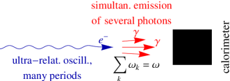
Figure 1: Scheme of gamma-radiation spectrum measurement yielding a multiphoton spectrum. The spent electron is deflected by a magnet, so only the forward-flying photons hit the calorimeter.

In view of appreciable difficulties with eliminating photon pileup effects, a common attitude at laboratory measurements of gamma-radiation spectra is not to pursue the objective of photon counting at all. Then, a single electromagnetic calorimeter is used to measure the total energy deposited by all the $\gamma$-quanta per event of electron passage through the radiator (see Fig. 1). Clearly, the latter method is equivalent to measuring the electron’s radiative energy loss spectrum. Furthermore, sometimes a simplified procedure of radiation spectrum measurement is adopted, when spent electron energies are measured, which then truly yields the spectrum of full energy losses by electrons in the radiator.

Even though the calorimetric method for spectrum measurement hinders applicability of formulas of classical electrodynamics, those can still be useful for the spectrum calculation. Indeed, the theory predicts that multiple soft photon emission probabilities factorize, expressing through the same classically calculated spectral intensity. To obtain the multiphoton spectrum, one thus needs to resum all $n$-photon probabilities while holding the total irradiated energy at a preselected value. Technically, the problem is similar to that of fast charged particle energy loss under statistically independent atom ionization acts in the medium Landau , and some other problems Bloch-Nordsieck ; EW-boson-resum ; Feller , whose solutions were attained by integral transform methods. For generic energy loss spectrum by a fast particle in the medium, a Laplace transform solution was known since 1944 Landau . In application to radiation, it was later utilized in Akh-Shul-shower-ZhETF , with the purpose of investigating soft (photon-dominated) electromagnetic showers in crystals and polycrystals, and checking the possibility of the shower length reduction due to coherent radiation effects. Relatively recently, in BK this method was used for studying the shape of the soft part of the radiation spectrum from electrons in an amorphous medium. Model solutions for shapes of synchrotron-like radiation spectra in crystals were discussed in Khokonov . There were also several investigations of shapes of radiation spectra in crystals, based on numerical simulation (usually by Monte-Carlo), with coh-rad-MCgenerators-negle+e- ; BKS-simul ; Artru-simul ; Kononets-Ryabov-simul ; Maisheev-simul or without coh-rad-MCgenerators-full neglect of $e^{+}e^{-}$ pair production as a first approximation.

Notwithstanding the pretty long history of the problem, there still remain many open questions concerning multiphoton effects on coherent radiation spectrum shapes. For example, since coherent radiation spectra are typically sharply peaked and discontinuous, the prime task is to investigate how do such features modify under multiphoton emission conditions. In so doing, it is also important to incorporate an incoherent bremsstrahlung component, which may require some special treatment, because of its divergent total probability. Next, it is important to give proper study for the behavior of the resummed coherent radiation spectrum in the high intensity (or photon multiplicity) limit. There, one generally expects the spectrum to tend to a Gaussian form, but corrections to this form may be significant at practice, and demand evaluation.

Besides the abovementioned most urgent problems, there is a number of developments which are desirable to make in the theory. First, it is expedient to supplement the notion of the resummed spectrum by that of photon multiplicity spectrum, which was proven measurable in experiments at CERN multiphot-CERN-Kirsebom . Secondly, it would be valuable for various purposes to find a possibility to reconstruct the single-photon spectrum from a calorimetrically measured one. Other issues include correspondence with the perturbation theory, separation of energetically ordered and anti-ordered contributions, etc.

The goal of the present paper is to provide a comprehensive formulation for the theory of resummed soft coherent radiation spectra, and with its aid, to tackle problems raised above. Although conditions of coherent radiation in different sources may vary, we concentrate on one of the most typical cases – dipole radiation (for overview of its conditions see, e.g., dipole-rad ), under the simplifying assumption of approximately harmonic transverse oscillation of the radiating electron (the neglect of higher harmonics). We incorporate also an incoherent radiation component, which, fortunately, has a simple structure, free from model assumptions. The interference between coherent and incoherent spectral components may be neglected in the first approximation. Therewith, there emerges a fairly model-independent description of radiation, which can embrace diverse practical situations.

This paper is laid out as follows. In Sec. II we establish main relations of the theory of soft multiphoton spectra. Along with the resummed spectrum itself, the photon multiplicity spectrum is defined. In Sec. III, the developed generic techniques are applied to the study of coherent and incoherent contributions to the radiation. Modification of various spectral features due to multiphoton effects, as well as interplay of coherent and incoherent radiation components, is investigated. Sec. IV explores the high-intensity limit, benefiting from the analogy between the multiphoton energy loss and a random walk. Having calculated the multiphoton spectrum in the central region, we also examine the spectrum behavior beyond it, and assess long-range effects due to the incoherent bremsstrahlung component. Sec. V works out the principles of reconstruction of the single-photon radiation spectrum from the calorimetrically measured one. The summary and some outlook is given in Sec. VI. A few technical issues are relegated to the Appendices.

II Generic resummation procedure

As was mentioned in the Introduction, for radiation emitted by an ultra-relativistic electron (or positron), the radiation angles are typically small (inversely proportional to the electron’s Lorentz factor), wherefore they often remain experimentally unresolved. In the latter case, only the radiation spectrum is measured. For coherent radiation, the spectrum is concentrated on a characteristic energy scale $\omega_{0}$, which is often much smaller than the initial electron energy $E_{e}$:

$$\omega_{0}\ll E_{e}.$$ (1)

Under those circumstances, the radiation recoils may be neglected, and the radiation process be treated as statistically independent emissions of photons by a classically moving charged particle. The description of the multiphoton spectrum then proceeds as follows.

II.1 Multiphoton spectra under statistically independent photon emission

Let the classically evaluated radiation energy spectrum, integrated over relativistically small emission angles, equal $\frac{dE_{1}}{d\omega}$. The corresponding photon number density could be derived as

$$\frac{dw_{1}}{d\omega}=\frac{1}{\omega}\frac{dE_{1}}{d\omega}.$$ (2)

That might as well be interpreted as the probability distribution for emission of a photon, but only provided its integral

$$w_{1}=\int_{0}^{\infty}d\omega\frac{dw_{1}}{d\omega},$$ (3)

which is to correspond to the total emission probability, is $\ll 1$. Sometimes the latter condition is fulfilled thanks to the smallness of electron coupling with the electromagnetic field, $\alpha=\frac{1}{137}$.

On the other hand, in a long radiator, $w_{1}$ can accumulate and get arbitrarily large. As it becomes sizable, proper probabilistic treatment must take into account emission of an arbitrary number of photons. Assuming that the radiation process remains soft and intrinsically semiclassical, photon emission acts can be proven to be statistically independent phot-stat-indep ; Poisson-rad , thereby obeying Poisson statistics:

$$\frac{dW_{n}}{d\omega_{1}\ldots d\omega_{n}}=W_{0}\frac{1}{n!}\frac{dw_{1}}{d\omega_{1}}\ldots\frac{dw_{1}}{d\omega_{n}}.$$ (4)

Here factors $W_{0}$ and $1/n!$ are consequences of probability conservation during photon generation. From the normalization of the total probability to unity,

$$W_{0}+\sum_{n=1}^{\infty}\int_{0}^{\infty}d\omega_{1}\ldots\int_{0}^{\infty}d\omega_{n}\frac{dW_{n}}{d\omega_{1}\ldots d\omega_{n}}=1,$$ (5)

one readily derives a relation of $W_{0}$ with the single-photon spectrum:

$$W_{0}=e^{-w_{1}}.$$ (6)

Since $W_{0}$ may be regarded as the 0-th term of the series, it is to be interpreted as the probability of photon non-emission. Quantity $w_{1}$ also admits an independent physical meaning, being equal to the mean number of emitted photons (the photon multiplicity):

$$\bar{n}=e^{-w_{1}}\sum^{\infty}_{n=1}\frac{n}{n!}w_{1}^{n}=w_{1}.$$ (7)

From the experimental point of view, completely exclusive spectrum $\frac{dW_{n}}{d\omega_{1}\ldots d\omega_{n}}$ is arguably too detailed. If we (idealistically) limit ourselves to a single-inclusive spectrum, where the energy of only one of the photons is measured, the corresponding observable would equal

$$W_{0}\sum_{n=1}^{\infty}\frac{1}{n!}\int_{0}^{\infty}\!d\omega_{1}\frac{dw_{1}}{d\omega_{1}}\ldots\int_{0}^{\infty}\!d\omega_{n}\frac{dw_{1}}{d\omega_{n}}\sum_{k=1}^{n}\delta\left(\omega-\omega_{k}\right)$$

$$=\frac{dw_{1}}{d\omega},\qquad\qquad\qquad\qquad\qquad\qquad\qquad\qquad$$ (8)

thus reproducing the photon number spectrum, connected with the classical energy spectrum via Eq. (2).

For the case of calorimetric measurement, however, the situation is different. There, the probability of emission of an arbitrary number of photons with definite aggregate energy $\omega$ is measured, taking the form

$$\frac{dw}{d\omega} = W_{0}\sum_{n=1}^{\infty}\frac{1}{n!}\int_{0}^{\infty}d\omega_{1}\frac{dw_{1}}{d\omega_{1}}\ldots$$ (9)

$$\qquad\qquad\times\int_{0}^{\infty}d\omega_{n}\frac{dw_{1}}{d\omega_{n}}\delta\left(\omega-\sum_{k=1}^{n}\omega_{k}\right).$$

The latter distribution is already properly normalized:

$$\int_{0}^{\infty}d\omega\frac{dw}{d\omega}=1-W_{0}.$$ (10)

As illustrated in Fig. 2, in the limit of low radiation intensity, distributions (II.1) and (9) match, since terms $n=1$ in their series are identical (Fig. 2a). But the rest of the terms, with $n\geq 2$, do differ (cf. Fig. 2b). Distribution (9) is often called multiphoton spectrum, and in contrast to that, (2) is called single-photon spectrum.

Figure 2: Integration domains for partial probabilities in Eqs. (II.1) and (9). (a) Component $n=1$. Only the point $\omega_{1}=\omega$ is selected by perfect detector of either kind. (b) Component $n=2$. Dashed lines mark the region selected by a perfect photon counter and spectrometer. Solid line, the region selected by a perfect calorimeter.

Another way of representing the results is via a multiphoton energy spectrum

$$\frac{dE_{\text{rad}}}{d\omega}:=\omega\frac{dw}{d\omega}\neq\frac{dE_{1}}{d\omega}.$$ (11)

In this paper, though, it will be advantageous for us to work with the probability spectral density. So, in what follows, the term ‘spectrum’ will mostly be used in relation to quantities such as $\frac{dw_{1}}{d\omega_{1}}$ and $\frac{dw}{d\omega}$.

Before proceeding with the resummation of series (9), it is expedient to inspect its structure more closely. First of all, in (9), upper integration limits for individual photon energies may actually be lowered down to $\omega$, granted that if energy of any of the emitted photons exceeds $\omega$, the energy-conserving $\delta$-function will definitely yield zero. At $n=1$, one yet needs to ensure that the $\delta$-function falls into the integration interval completely, so the integration upper limit should be written more precisely as $\omega+0$. With the forthcoming resummation procedure in mind, it is convenient to let the upper integration limit be the same everywhere, writing:

$$\frac{dw}{d\omega}=W_{0}\sum_{n=1}^{\infty}\frac{1}{n!}\int_{0}^{\omega+0}d\omega_{1}\frac{dw_{1}}{d\omega_{1}}\ldots\qquad\qquad\qquad$$

$$\times\int_{0}^{\omega+0}d\omega_{n}\frac{dw_{1}}{d\omega_{n}}\delta\left(\omega-\sum_{k=1}^{n}\omega_{k}\right).$$ (12)

Next, even though in Eq. (II.1) upper integration limits for partial probabilities are rendered finite, in integral (3) entering $W_{0}$ through Eq. (6), the integration extends over an infinite range of $\omega_{1}$. That fact needs care, since at $\omega\sim E_{e}$, quantum corrections due to photon recoils invalidate the statistical independence of photon emission acts. For pure coherent radiation, whose spectrum is strongly suppressed beyond a sufficiently low energy $\omega_{0}$, such a problem may be absent. However, there often exists an incoherent bremsstrahlung contribution to $\frac{dw_{1}}{d\omega_{1}}$, scaling as $\frac{dw_{1}}{d\omega_{1}}\propto\omega_{1}^{-1}$. Therewith, integral $w_{1}$ logarithmically diverges on the upper limit, whereby factor $e^{-w_{1}}$ would nullify the multiphoton radiation spectrum for any finite $\omega$, if there was no physical end of the bremsstrahlung spectrum, situated at $\omega=E_{e}$. Within the leading logarithmic (LL) accuracy, the upper integration limit could be merely replaced by $E_{e}$:

$$w_{1}\simeq\int_{0}^{E_{e}}d\omega_{1}\frac{dw_{1}}{d\omega_{1}}\qquad(\text{LL accuracy}).$$ (13)

However, the usage of the leading-log accuracy in Eq. (4), where $w_{1}$ is exponentiated, may be unsatisfactory, as long as it introduces an indeterminate overall factor. Thence, it is worth promoting it to the next-to-leading logarithmic (NLL) accuracy. That is equivalent to effectively replacing Eq. (13) by

$$w_{1}\simeq\int_{0}^{E}d\omega_{1}\frac{dw_{1}}{d\omega_{1}}\qquad(\text{NLL accuracy}),$$ (14)

where parameter $E=\kappa E_{e}\sim 1$ must be ab initio calculable in NLL. A study delivered in Appendix A (though still under the neglect of pair production) suggests that $\kappa\approx 0.5$. Greater accuracy may be unnecessary, since $\kappa$ only enters in terms a power $\kappa^{a}$ with $a\ll 1$ (see Sec. III.1).

The incoherent bremsstrahlung contribution also dominates in the opposite extreme $\omega_{1}\to 0$, where its behavior $\frac{dw_{1}}{d\omega_{1}}\sim\omega_{1}^{-1}$ makes all the integrals present in Eq. (II.1) diverge on the lower limit. Fortunately, though, the infrared (IR) divergence cancels for energy-resummed distributions by virtue of the Bloch-Nordsieck theorem phot-stat-indep ; Bloch-Nordsieck , as will be demonstrated in the next subsection.

II.2 Contour integral representations

Resummation of series of type (9) proceeds by applying a Laplace transform, which reduces the multiple convolution to a simple product of equal single integrals, and the resulting power series resums to an exponential:

$$\int_{0}^{\infty}d\omega\frac{dw}{d\omega}e^{-s\omega} = e^{-w_{1}}\sum_{n=1}^{\infty}\frac{1}{n!}\prod_{k=1}^{n}\int_{0}^{E}d\omega_{k}\frac{dw_{1}}{d\omega_{k}}e^{-s\omega_{k}}$$ (15)

$$= e^{\int_{0}^{E}d\omega_{1}\frac{dw_{1}}{d\omega_{1}}\left(e^{-s\omega_{1}}-1\right)}-W_{0}.$$

[Prior to the resummation, we implemented a proper cutoff parameter $E$, in the manner of Eq. (14)]. An immediate observation from Eq. (15) is that by virtue of factor $e^{-s\omega_{1}}-1$ tending to zero as $\omega_{1}\to 0$, the infrared singularity brought by $\frac{dw_{1}}{d\omega_{1}}$ is suppressed, providing the integral convergence on the lower limit if $\frac{dw_{1}}{d\omega_{1}}=\mathcal{O}(\omega_{1}^{-1})$. If $s$ is put to zero, Eq. (15) reproduces normalization condition (10).

The Laplace transform is further inverted by computing a Mellin integral in the complex $s$-plane:

$$\frac{dw}{d\omega}=\frac{1}{2\pi i}\int_{c-i\infty}^{c+i\infty}dse^{s\omega}\int_{0}^{\infty}d\omega_{1}\frac{dw}{d\omega_{1}}e^{-s\omega_{1}}.$$ (16)

Here constant $c$ is required to be greater than real parts of all singularities of the integrand, otherwise being arbitrary. Combining Eqs. (16) and (15) yields the generic integral representation for the multiphoton radiation spectrum:

$$\frac{dw}{d\omega}=\frac{1}{2\pi i}\int_{c-i\infty}^{c+i\infty}dse^{s\omega+\int_{0}^{E}d\omega_{1}\frac{dw_{1}}{d\omega_{1}}\left(e^{-s\omega_{1}}-1\right)}-W_{0}\delta(\omega).$$ (17)

The appearance in Eq. (17) of a negative term proportional to Dirac $\delta$-function does not imply negativity of the resummed spectrum at $\omega=0$. It just cancels the corresponding positive singularity in the contour integral, arising because its integrand tends to $W_{0}e^{s\omega}$ as $s\to\pm i\infty$. At $\omega>0$, the $\delta$-term does not contribute, anyway, but it proves important at derivation of various integral relations involving $\frac{dw}{d\omega}$ [in particular, maintaining the correct normalization (10)]. The integral on the r.h.s. of (17),

$$\frac{dw}{d\omega}+W_{0}\delta(\omega)=\Pi(E_{e}-\omega),$$ (18)

has an independent physical meaning, representing the distribution function for the radiating electrons, which is singular at $\omega=0$, but is normalized to unity:

$$\int_{0}^{\infty}d\omega\left\{\frac{dw}{d\omega}+W_{0}\delta(\omega)\right\}=1.$$ (19)

Representation (17) without the $\delta$-term, i.e. holding for function $\Pi(E_{e}-\omega)$ [or pertaining to case $w_{1}=\infty$, $W_{0}\equiv 0$], was derived by Landau Landau on the basis of a kinetic equation.

Next, let us note that contour integral representation (17) needs not be the only possible one. The example of representation (II.1) shows that in the exponentiated Laplace transform of $\frac{dw_{1}}{d\omega_{1}}$, the upper integration limit may be arbitrary, provided it exceeds $\omega$. For instance, lowering it right down to $\omega$ leads to the integral representation

$$\frac{dw}{d\omega}=e^{-\!\int^{E}_{\omega}\!d\omega_{1}\!\frac{dw_{1}}{d\omega_{1}}}\frac{1}{2\pi i}\int_{c-i\infty}^{c+i\infty}\!dse^{s\omega+\int_{0}^{\omega+0}\!d\omega_{1}\!\frac{dw_{1}}{d\omega_{1}}\!\left(\!e^{-s\omega_{1}}-1\!\right)}$$

$$-W_{0}\delta(\omega).\qquad\qquad\qquad\qquad\qquad\qquad\qquad$$ (20)

Indeed, expanding here $e^{\int_{0}^{\omega+0}d\omega_{1}\frac{dw_{1}}{d\omega_{1}}e^{-s\omega_{1}}}$ to Taylor series and integrating over $s$ termwise leads to decomposition (II.1). Relation (II.2) was first noticed in BK , wherein it was regarded as only an approximate consequence of representation (17) (in the sense that in the integral over $s$, the contributing $s$ are $\sim\omega^{-1}$, and hence in $\int_{0}^{E}d\omega_{1}\frac{dw_{1}}{d\omega_{1}}e^{-s\omega_{1}}$ the contributing $\omega_{1}$ are $\lesssim s^{-1}\sim\omega$). But here, by deriving both representations (17) and (II.2) from the same series, we reveal their exact equivalence.

Although the derivation of representation (II.2) given above is illuminating, it may be desirable sometimes to avoid the use of power series, which may be beset by IR divergences. In that case, one may utilize the following generic statement:

Lemma 1.

Let $\omega\geq\epsilon\geq 0$ be real parameters, and $f(\omega_{1})$ be a positive function of real variable, integrable on interval $\epsilon<\omega_{1}<\infty$. Also let $\mathcal{F}(z)$ be an analytic function of complex variable $z$ in domain $\mathfrak{Re}z>0$, and such that $\left|\mathcal{F}^{\prime}\left(\int_{\epsilon}^{\omega+\varpi}d\omega_{1}e^{-s\omega_{1}}f(\omega_{1})\right)\right|$ grows with $\mathfrak{Re}s\to+\infty$ slower than exponentially. Then, contour integral

$$\int_{c-i\infty}^{c+i\infty}dse^{s\omega}\mathcal{F}\left(\int_{\epsilon}^{\omega\!+\!\varpi}d\omega_{1}e^{-s\omega_{1}}f(\omega_{1})\!\right)\!,\,$$ (21)

where $\mathfrak{Re}c$ is greater than real parts of all singularities of the integrand in the $s$-plane, is independent of $\varpi$ on the semiaxis $\varpi>0$.

Proof.

Differentiation of Eq. (21) by parameter $\varpi$ gives:

$$\frac{\partial}{\partial\varpi}\int_{c-i\infty}^{c+i\infty}\!dse^{s\omega}\mathcal{F}\left(\int_{\epsilon}^{\omega+\varpi}d\omega_{1}e^{-s\omega_{1}}f(\omega_{1})\!\right)\qquad\qquad$$

$$=f(\omega+\varpi)\!\int_{c-i\infty}^{c+i\infty}\!dse^{-\varpi s}\mathcal{F}^{\prime}\!\left(\int_{\epsilon}^{\omega+\varpi}\!\!d\omega_{1}e^{-s\omega_{1}}f(\omega_{1})\!\right).$$

The condition that function $\left|\mathcal{F}^{\prime}\left(\int_{\epsilon}^{\omega+\varpi}d\omega_{1}e^{-s\omega_{1}}f(\omega_{1})\right)\right|$ grows with $\mathfrak{Re}s$ slower than exponentially guarantees the exponential decrease of the integrand of (II.2) when $\varpi>0$. Thus, if the integration contour, defined to pass on the right of all singularities of the integrand, is withdrawn rightwards to infinity, the whole integral exponentially vanishes. Therewith, derivative (II.2) is identically zero, which entails independence of integral (21) on $\varpi$ under the conditions assumed. ∎

In our case (17), (II.2), function $\mathcal{F}(z)$ has to be identified with an exponential

$$\mathcal{F}(z)=e^{z-\int_{\epsilon}^{E}d\omega_{1}\frac{dw_{1}}{d\omega_{1}}}\equiv\mathcal{F}^{\prime}(z)$$ (23)

(where $\epsilon$ furnishes an IR cutoff, if necessary). Function (23) satisfies the conditions of our lemma liberally: since $z(s)=\int^{E}_{\epsilon}d\omega_{1}e^{s\omega_{1}}\frac{dw_{1}}{d\omega_{1}}$ increases at $\mathfrak{Re}s\to+\infty$ at most logarithmically, $|\mathcal{F}^{\prime}[z(s)]|$ in this limit can only increase as some power of $s$. As a whole, $\mathcal{F}(z)$ is actually IR-finite, so after unifying $\omega_{1}$-integrals in the exponent of $\mathcal{F}$, it is safe to put $\epsilon=0$. By choosing in expression (21) $\varpi$ arbitrarily small or large, one can deduce Eq. (II.2) from Eq. (17), or vice versa. We will also employ Lemma 1 for simplification of the exponentiated integrals with specific profiles of $dw_{1}/d\omega_{1}$ in the next section.

Eq. (II.2) has an appealing property that apart from the factor

$$e^{-\int^{E}_{\omega}d\omega_{1}\frac{dw_{1}}{d\omega_{1}}}=W_{0}(\omega),$$ (24)

the multiphoton spectrum involves only contributions from the single-photon spectrum with $\omega_{1}<\omega$. That looks natural in view of the positivity of contributing photon energies. In this sense, it seems natural to term Eq. (II.2) ‘energetically ordered’ form [to distinguish it from ‘non-ordered’ form (17)]. Still, one should mind the existence of factor (24), which depends on contributions from $\omega_{1}>\omega$, and is nothing but the probability of non-emission of any photon with energy greater than $\omega$ BK (check:

$$W_{0}+\sum_{n=1}^{\infty}\int_{0}^{\infty}d\omega_{1}\ldots\int_{0}^{\infty}d\omega_{n}\frac{dW_{n}}{d\omega_{1}\ldots d\omega_{n}}\prod_{k=1}^{n}\theta(\omega-\omega_{k})$$

$$=W_{0}(\omega),\qquad\qquad\qquad\qquad\qquad\qquad\qquad\qquad\qquad$$

with $\theta$ standing for the Heaviside unit step function). So, the effect of contributions from $\omega_{1}>\omega$ is ‘non-dynamical’, resulting in a rather trivial explicit factor, but nonetheless, due to this factor, the energetic ordering does not hold strictly for multiphoton probability spectrum. Remarkably, in Sec. V we will encounter representations which may be regarded even as energetically anti-ordered.

II.3 Perturbation series

The manifestation of multiphoton effects may be studied in terms of non-linearity of the radiation spectrum dependence on the radiator length (or the crystalline target thickness), $L$ (cf. relevance-of-multiphot ; relevance-of-multiphot2 ). In the simplest approximation (reasonable for long radiators), one may assume that $\frac{dw_{1}}{d\omega_{1}}\propto L$. Then, $L$-dependence of $\frac{dw}{d\omega}$ may be studied based on expansion (9), where factor $W_{0}$ is yet a non-linear function of $w_{1}$. Expanding the latter factor to series in $w_{1}$ leads to a double series for $\frac{dw}{d\omega}$.

In fact, a single power series in $L$ can be obtained using the following trick. Issuing from contour integral representation (17), integrate in the exponent by parts:

$$\frac{dw}{d\omega} = \frac{1}{2\pi i}\int_{c-i\infty}^{c+i\infty}dse^{s\omega-s\int_{0}^{E}d\omega_{1}e^{-s\omega_{1}}\int^{E}_{\omega_{1}}d\omega^{\prime}_{1}\frac{dw_{1}}{d\omega^{\prime}_{1}}}$$ (25)

$$-W_{0}\delta(\omega).$$

Next, expand the $\frac{dw_{1}}{d\omega_{1}}$-dependent part of the exponential to power series:

$$\frac{dw}{d\omega}=\sum^{\infty}_{n=1}\frac{dw_{n}}{d\omega},$$ (26)

with

$$\frac{dw_{n}}{d\omega} = \frac{(-1)^{n}}{n!}\frac{1}{2\pi i}\int_{c-i\infty}^{c+i\infty}dss^{n}e^{s\omega}$$

$$\times\prod^{n}_{k=1}\int_{0}^{E}d\omega_{k}e^{-s\omega_{k}}\int_{\omega_{k}}^{E}d\omega^{\prime}_{k}\frac{dw_{1}}{d\omega^{\prime}_{k}}.$$

Now, it is straightforward to integrate over $s$ termwise with the use of the identity

$$\frac{1}{2\pi i}\int_{c-i\infty}^{c+i\infty}dse^{s\left(\omega-\sum_{k=1}^{n}\omega_{k}\right)}s^{n}=\frac{\partial^{n}}{\partial\omega^{n}}\delta\left(\omega-\sum_{k=1}^{n}\omega_{k}\right),$$ (27)

which yields

$$\frac{dw_{n}}{d\omega}=\frac{(-1)^{n}}{n!}\frac{\partial^{n}}{\partial\omega^{n}}\int_{0}^{E}d\omega_{1}\ldots\int_{0}^{E}d\omega_{n}\qquad\qquad\quad$$

$$\times\delta\left(\omega-\sum_{k=1}^{n}\omega_{k}\right)\int^{E}_{\omega_{1}}d\omega^{\prime}_{1}\frac{dw_{1}}{d\omega^{\prime}_{1}}\ldots\int^{E}_{\omega_{n}}d\omega^{\prime}_{n}\frac{dw_{1}}{d\omega^{\prime}_{n}}.\quad$$ (28)

The latter multiple integral converges even if the mean photon number $w_{1}$ diverges logarithmically; its multiple derivatives always exist, as well.

In contrast to Eq. (9), however, terms of series (II.3) need not be everywhere positive. That is chained to the fact that multiple photon emission leads to a redistribution of the spectrum, not only to pileup of events. From the standpoint of QED, negative terms in the perturbative expansion typically arise from interference of loop (photon reabsorption) diagrams with lower-order ones phot-stat-indep . Eq. (II.3) indicates that for an observable such as the calorimetrically measured spectrum, the structure of those corrections assumes a simple generic form.

Correspondence of (II.3) with expansion (9) may be established by differentiating in (II.3) the delta-function under the integral sign by formula

$$(-1)^{n}\frac{\partial^{n}}{\partial\omega^{n}}\delta\left(\!\omega-\sum_{k=1}^{n}\omega_{k}\!\right)=\frac{\partial^{n}}{\partial\omega_{1}\ldots\partial\omega_{n}}\delta\left(\!\omega-\sum_{k=1}^{n}\omega_{k}\!\right)\!,$$ (29)

and subsequently integrating by parts over all $\omega_{k}$. It should be minded thereat that the endpoint terms are non-vanishing, producing the powers of the total single-photon emission probability $w_{1}$ present in Eq. (9) in the exponent. However, if $w_{1}$ diverges, the integration by parts is no longer possible, wherewith series (9) does not exist, but Eq. (II.3) remains valid, anyway.

II.4 Spectral moments

Characterization of compact probability distributions is often conducted in terms of their moments. Spectrum $\frac{dw}{d\omega}$, however, is not normalized to unity, so it can not be used straightforwardly as a weighting distribution. In capacity of a normalized probability distribution, one should either use electron distribution function (18), or the rescaled radiation spectrum $\frac{1}{1-W_{0}}\frac{dw}{d\omega}$. We will adopt the first option, which leads to simpler final results.

The mean emitted photon energy for our resummed spectrum is computed, e.g., by termwise integration in Eq. (9):

$$\overline{\omega} = \int_{0}^{\infty}d\omega\omega\left[\frac{dw}{d\omega}+W_{0}\delta(\omega)\right]\equiv\int_{0}^{\infty}d\omega\omega\frac{dw}{d\omega}$$ (30)

$$= e^{-w_{1}}\sum_{n=1}^{\infty}\frac{n}{n!}w_{1}^{n-1}\overline{\omega_{1}\!}=\overline{\omega_{1}\!}.$$

Thus, it coincides with that for the single-photon spectrum,

$$\overline{\omega_{1}\!}=\int_{0}^{\infty}d\omega_{1}\omega_{1}\frac{dw_{1}}{d\omega_{1}}.$$ (31)

That is quite natural, inasmuch as once photon energies in all the events are summed over, it no longer matters whether they were measured by photon counters or calorimeters. [In particular, that justifies the use of classical formulas for the rate of radiative energy losses (see, e.g., mean-energy-loss ) under conditions of multiple photon emission.]

To further characterize the spectrum width, asymmetry, and so on, one can refer to higher moments about the mean value (central moments), presuming their existence. Those are conveniently calculated based on representation (17):

$$\overline{(\omega-\overline{\omega})^{n}} = \int_{0}^{\infty}d\omega(\omega-\overline{\omega_{1}\!})^{n}\left[\frac{dw}{d\omega}+W_{0}\delta(\omega)\right]\qquad\qquad$$ (32)

$$= \left(-\frac{\partial}{\partial s}-\overline{\omega_{1}\!}\right)^{n}e^{\int_{0}^{E}d\omega_{1}\frac{dw_{1}}{d\omega_{1}}\left(e^{-s\omega_{1}}-1\right)}\bigg{|}_{s=0}$$

$$\equiv (-1)^{n}\frac{\partial^{n}}{\partial s^{n}}e^{\int_{0}^{E}d\omega_{1}\frac{dw_{1}}{d\omega_{1}}\left(e^{-s\omega_{1}}-1+s\omega_{1}\right)}\bigg{|}_{s=0}.\,\,$$

The above representation implies that exponential $e^{\int_{0}^{E}d\omega_{1}\frac{dw_{1}}{d\omega_{1}}\left(e^{-s\omega_{1}}-1+s\omega_{1}\right)}$ serves as a generating function Gnedenko-Kolmogorov ; Feller for central moments, while $e^{\int_{0}^{E}d\omega_{1}\frac{dw_{1}}{d\omega_{1}}\left(e^{-s\omega_{1}}-1\right)}$ offers a generating function for ordinary moments. Applying Eq. (32) for lowest $n$, one finds

$$\overline{\left(\omega-\overline{\omega}\right)^{2}}=\overline{\omega_{1}^{2}},$$ (33)

$$\overline{\left(\omega-\overline{\omega}\right)^{3}}=\overline{\omega_{1}^{3}},$$ (34)

$$\overline{\left(\omega-\overline{\omega}\right)^{4}}=3\big{(}\overline{\omega_{1}^{2}}\big{)}^{2}+\overline{\omega_{1}^{4}},$$ (35)

etc. Relations (30), (33) (historically known as Campbell’s theorem Feller ) were discussed in Kolchuzhkin with the objective of extracting information about the single-photon distribution from the resummed one. Eqs. (34), (35) may serve for the same purpose. In addition, in Sec. V we will formulate a reconstruction procedure for the complete spectrum, not resorting to the notion of moments.

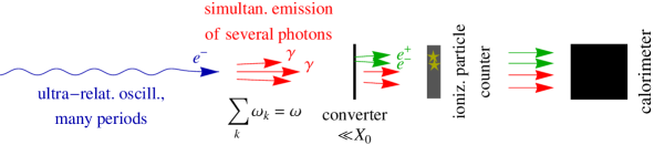
Figure 3: Scheme of measurement of the photon multiplicity spectrum. Due to the converter thinness, the number of $e^{+}e^{-}$ pairs created in it is proportional to the number of incident photons. The knowledge of the proportionality coefficient then allows assessing the photon number in a radiative event. The total energy emitted per event is measured by the final calorimeter, as in Fig. 1.

A predicament with the use of the above quoted moments is that with the account of an incoherent bremsstrahlung component (Sec. III), they all diverge in the ultraviolet. Therefore, they may seem to be only useful in the context of pure coherent radiation. Nonetheless, later on we will show that treatments of coherent and incoherent radiation components can always be separated, permitting the usage of spectral moments for pure coherent component regardless of the presence of an incoherent one.

II.5 Photon multiplicity spectrum

As was mentioned in the Introduction, it is rather difficult in a multiphoton event to practically pin down individual energies of all the photons, i.e., to measure joint probability distribution $\frac{dW_{n}}{d\omega_{1}\ldots d\omega_{n}}$. But there exist relatively compact experimental methods allowing to receive partial information about the photon number content. For instance, placement of a thin converter and an ionizing particle counter upstream the calorimeter allows measuring the mean number of photons (the photon multiplicity) as a function of the total energy $\omega$ deposited in the calorimeter – see Fig. 3 and, e.g., multiphot-CERN-Kirsebom . In this subsection, we will extend our resummation procedure to description of the photon multiplicity spectrum.

In the spirit of Eqs. (7) and (9), to construct the photon multiplicity at a given $\omega$, one must incorporate in (9) a weighting factor $n$ equal to the number of emitted photons, whereupon divide the resulting sum by the unweighted expression:

$$\bar{n}(\omega)=\frac{W_{0}}{dw/d\omega}\sum_{n=1}^{\infty}\frac{n}{n!}\int_{0}^{\infty}d\omega_{1}\frac{dw_{1}}{d\omega_{1}}\ldots\qquad$$

$$\times\int_{0}^{\infty}d\omega_{n}\frac{dw_{1}}{d\omega_{n}}\delta\left(\omega-\sum_{k=1}^{n}\omega_{k}\right).$$ (36)

Since all the weights $n$ in this sum are greater than unity, so must be their mean number:

$$\bar{n}(\omega)\geq 1.$$ (37)

In particular, when $\omega\to 0$, integration phase space volumes for $n\geq 2$ terms shrink to zero, wherefore only term $n=1$ survives. This term cancels with the correspondent term in the denominator, yielding

$$\bar{n}(0)=1.$$ (38)

The sum entering Eq. (II.5) can again be evaluated by the Laplace transform method, as follows:

$$\bar{n}(\omega)\frac{dw}{d\omega} = \frac{1}{2\pi i}\int_{c-i\infty}^{c+i\infty}dse^{s\omega+\int_{0}^{E}d\omega_{1}\frac{dw_{1}}{d\omega_{1}}\left(e^{-s\omega_{1}}-1\right)}\quad$$

$$\qquad\qquad\quad\times\int_{0}^{E}d\omega^{\prime}_{1}\frac{dw_{1}}{d\omega^{\prime}_{1}}e^{-s\omega^{\prime}_{1}}$$

$$\equiv \frac{W_{0}(\omega)}{2\pi i}\int_{c-i\infty}^{c+i\infty}dse^{s\omega+\int_{0}^{\omega}d\omega_{1}\frac{dw_{1}}{d\omega_{1}}\left(e^{-s\omega_{1}}-1\right)}\quad$$

$$\qquad\qquad\quad\times\int_{0}^{\omega}d\omega^{\prime}_{1}\frac{dw_{1}}{d\omega^{\prime}_{1}}e^{-s\omega^{\prime}_{1}}.$$ (39b)

[The latter equality may be inferred from Lemma 1 with $\mathcal{F}(z)=ze^{z-\int_{0}^{E}d\omega_{1}\frac{dw_{1}}{d\omega_{1}}}$]. This may also be expressed as a convolution of the single-photon spectrum with the resummed one:

$$\bar{n}(\omega)\frac{dw}{d\omega}=\int_{0}^{\omega}d\omega_{1}\frac{dw_{1}}{d\omega_{1}}\frac{dw}{d\omega^{\prime}}\bigg{|}_{\omega^{\prime}=\omega-\omega_{1}}+W_{0}\frac{dw_{1}}{d\omega}.$$ (40)

Here the last term stems from the $\delta$-function term of Eq. (II.2).

Unlike $\frac{dw}{d\omega}$, however, the multiplicity spectrum is not an IR-safe quantity. But fortunately, the IR divergence of $w_{1}$ affects only the constant, $\omega$-independent part of $\bar{n}(\omega)$. Indeed, the contribution from vicinity of the lower integration limit in the convolution term in (40) is $\propto dw/d\omega$, and so is the l.h.s. Hence, at $W_{0}\to 0$, $\omega$-dependent factors in both sides of Eq. (40) cancel.

To isolate the IR divergence of $\bar{n}(\omega)$ explicitly, one can rewrite Eq. (40), e.g., as

$$\bar{n}(\omega)-\!\int_{\epsilon}^{\omega}\!d\omega_{1}\frac{dw_{1}}{d\omega_{1}}=\int_{0}^{\omega}\!d\omega_{1}\frac{dw_{1}}{d\omega_{1}}\!\left(\frac{\frac{dw}{d\omega^{\prime}}\big{|}_{\omega^{\prime}=\omega-\omega_{1}}}{{dw}/{d\omega}}-1\!\right)$$

(41)

$$(w_{1}\to\infty).\qquad\qquad\qquad\qquad\qquad$$

Here the r.h.s. is IR-safe (thence we put there $\epsilon=0$), while in the l.h.s., the dependence of $\bar{n}(\omega)$ on the IR cutoff $\epsilon$ must be additive, to cancel with the additive dependence on IR cutoff of the integral term. On the other hand, the dependence of on $E$ for $\bar{n}(\omega)$ must disappear, as will be demonstrated in the next section.

III Properties of incoherent and coherent multiphoton radiation spectra

Generic resummation formulas established in the previous section are valid for radiation characterized by an arbitrary single-photon profile $dw_{1}/d\omega_{1}$. In what follows, we will mostly concentrate on a category of coherent radiation spectra involving an admixture of incoherent radiation. In that case, the salient features shared by the single-photon spectra are:

• spectral discontinuities at finite $\omega$ in the coherent radiation component (coherent emission edges);

• a ‘tail’ towards large $\omega$ brought by the incoherent bremsstrahlung component;

• an infrared divergence, originating from the incoherent bremsstrahlung, or from non-zero net deflection by coherent fields (see, e.g., Bondarenco-CBBC ). For simplicity, in this paper we will be only considering the first case.

Our first task is to investigate how do the above mentioned features modify under multiphoton emission conditions. Since multiphoton effects interplay nonlinearly, it is expedient first to analyze them for pure coherent and incoherent components separately. Combining them, we can thereupon distinguish effects of their mutual influence.

III.1 Pure incoherent bremsstrahlung

Let us first scrutinize the case of purely incoherent bremsstrahlung. Its single-photon spectrum must be proportional to Bethe-Heitler’s spectrum of radiation at a single collision Rossi . Moreover, in the soft radiation limit we are restricted to, the single-photon spectrum reduces to the well-known semiclassical form 1/omega-spectrum

$$\frac{dw_{1\text{i}}}{d\omega_{1}}\simeq\frac{a}{\omega_{1}}\qquad(\omega_{1}\ll E_{e}),$$ (42)

where $a$ is proportional to the target thickness $L$. In an amorphous matter, constant $a$ equals

$$a=\frac{4}{3}\frac{L}{X_{0}},$$ (43)

where the radiation length $X_{0}\approx(4Z^{2}\alpha r_{e}^{2}n_{\text{a}}\ln\frac{1}{Z^{1/3}\alpha})^{-1}$ depends on the atomic density $n_{\text{a}}$ and (net) nucleus charge $Z$ Rossi ; PDG . A similar estimate applies also for the incoherent component of coherent bremsstrahlung in a crystal. For the case of positron channeling, if their close collisions with atomic nuclei are sufficiently rare, factor $Z^{2}n_{\text{a}}$ should be replaced by the net interplanar electron density $n_{e}$. Finally, in an undulator, $a$ is proportional to the density of the residual air, though in high vacuum that can be negligible.

As was argued in the end of Sec. II.1, the integral of (42), which is logarithmically divergent in the UV, must be cut off at some photon energy commensurable with the electron energy: $E=\kappa E_{e}$, with $\kappa\sim 0.5$. We implement this cutoff directly for approximation (42), adopting a simplified model:

$$\frac{dw_{1\text{i}}}{d\omega_{1}}=\frac{a}{\omega_{1}}\theta(E-\omega_{1}),$$ (44)

where $\theta(z)$ is the Heaviside function.

Figure 4: Integration contours for resummed spectra. Line $\mathcal{C}_{1}$, used in Eq. (17), (II.2). Deformed contour $\mathcal{C}_{2}$, used in Eqs. (48), (82). Closed loop contour $\mathcal{C}_{3}$, applicable for pure coherent radiation (see Sec. III.2.1).

A convenient starting point for evaluation of the resummed spectrum corresponding to single-photon spectrum (44) is the energetically ordered contour integral representation, Eq. (II.2). Therein, the $\delta$-term is suppressed, since $W_{0}\to 0$, and for the present case it will be neglected. Once (44) is inserted to Eq. (II.2), all $\omega$- and $E$-dependencies factor out after a simple rescaling of the integration variables, giving

$$\frac{dw_{\text{i}}}{d\omega}=\frac{a}{\omega}\left(\frac{\omega}{E}\right)^{a}\Phi(a)\equiv\frac{dw_{1\text{i}}}{d\omega}\left(\frac{\omega}{E}\right)^{a}\Phi(a)\qquad(\omega<E),$$ (45)

with

$$\Phi(a)=\frac{1}{a}\frac{1}{2\pi i}\int_{c-i\infty}^{c+i\infty}d\zeta e^{\zeta+a\int_{0}^{1}\frac{d\xi}{\xi}\left(e^{-\zeta\xi}-1\right)}.$$ (46)

To evaluate $\Phi(a)$, one may regularize $\int\frac{d\xi}{\xi}\left(e^{-\zeta\xi}-1\right)$ on the lower limit, then split it in two integrals, and by Lemma 1, extend the upper limit of the integral involving $e^{-\zeta\xi}$ to infinity. Thereafter, the IR regulator may again be sent to zero, and the sum of $\xi$-integrals evaluates:

$$\Phi(a)=e^{a\int_{0}^{\infty}dze^{-z}\ln z}\frac{1}{a}\frac{1}{2\pi i}\int_{c-i\infty}^{c+i\infty}\frac{d\zeta}{\zeta^{a}}e^{\zeta}.$$ (47)

The integrand of the latter contour integral is vanishing as $\mathfrak{Re}\zeta\to-\infty$, so at complex infinity the contour can be turned to the left from the imaginary axis (contour $\mathcal{C}_{2}$ in Fig. 4). Using representation

$$\frac{1}{\Gamma(a)}=\frac{1}{2\pi i}\int_{\mathcal{C}_{2}}\frac{d\zeta}{\zeta^{a}}e^{\zeta}$$ (48)

for the Euler gamma function, and definition

$$-\int_{0}^{\infty}dze^{-z}\ln z\equiv-\Gamma^{\prime}(1)=\gamma_{\text{E}}=0.577\ldots$$

for Euler’s constant, we get

$$\Phi(a)=\frac{e^{-\gamma_{\text{E}}a}}{\Gamma(1+a)}.$$ (49)

Function (49) is manifestly positive and monotonously decreasing (see Fig. 5), its derivative in the origin being zero:

$$\Phi(a)=1-\frac{\pi^{2}}{12}a^{2}+\mathcal{O}(a^{3}).$$

Other models for the single-photon spectrum suppression at large $\omega_{1}$ yield equivalent results.

Regarding the shape of the resulting distribution, two remarks are in order. First, spectrum (45) is suppressed compared to single-photon spectrum (42) everywhere in the region $\omega<E$. At $\omega>E$, there formally develops an enhancement of the spectrum, but it is not accurately described by Eq. (45), insofar as at $\omega\sim E$ quantum effects enhance, while at $\omega=E_{e}$, the spectrum must strictly terminate at all. Hence, there ansatz (44) for the single-photon spectrum breaks down, so our model description, though self-consistent formally, is inadequate in domain $\omega\sim E$. With this reservation, the uniform suppression of the resummed spectrum at $\omega<E$ does not contradict, e.g., the conservation of the mean photon energy at resummation [Eq. (30)].

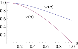
Figure 5: Graphs of functions $\Phi(a)$ [Eq. (49)] and $\nu(a)$ [Eq. (56b)]. Our physical assumptions require that $a\ll 1$ (see text).

Secondly, the dependence of the resummed spectrum on $\kappa$ enters Eq. (45) through parameter $E=\kappa E_{e}$, resulting in an overall factor $\kappa^{-a}$. Thus, in order for result (45) not to be strongly sensitive to the actual value of $\kappa$, one needs fulfillment of condition

$$a\ll 1$$ (51)

(otherwise, full kinetic equations for the electromagnetic cascade will need to be solved). Since the accuracy of Eq. (45) is $[\mathcal{O}(1)]^{a}=1+\mathcal{O}(a)$, function $\Phi(a)=\Phi(0)+\mathcal{O}(a^{2})$ may be safely approximated by $\Phi(0)=1$. Then, one readily checks that

$$\int_{0}^{E}d\omega\frac{dw_{\text{i}}}{d\omega}=\Phi(a)\underset{a\ll 1}{\approx}1,$$ (52)

in accord with Eq. (10) (where, again, $W_{0}\to 0$, owing to IR divergence of $w_{1\text{i}}$). Property (52) implies that despite the smallness of $a$, function (45) is not uniformly small, but rather is similar to a $\delta$-function, peaking at $\omega\to 0$ where function (45) blows up:

$$\underset{a\to 0}{\lim}\frac{dw_{\text{i}}}{d\omega}=\delta(\omega).$$ (53)

To prove Eq. (53), and estimate the narrowness of $\frac{dw_{\text{i}}}{d\omega}$ as a function of parameter $a$, it may be expedient to evaluate a median energy $\omega_{\text{i}\frac{1}{2}}$ at which there accumulates half probability of the resummed incoherent radiation, i.e.

$$\int_{0}^{\omega_{\text{i}\frac{1}{2}}}d\omega\frac{dw_{\text{i}}}{d\omega}:=\frac{1}{2}.$$

That yields

$$\omega_{\text{i}\frac{1}{2}}=\left[2\Phi(a)\right]^{-1/a}E\lll E_{e},$$ (54)

which at small $a$ is exponentially small, thereby validating relation (53).

Finally, the (regularized) photon multiplicity spectrum can be evaluated for the present case via Eq. (II.5). Inserting (42) and (45) to (II.5), and evaluating the integral, we get:

$$\bar{n}_{\text{i}}(\omega)=a\ln\frac{\omega}{\epsilon}+\nu(a),$$ (55)

with

$$\nu(a) = a\int_{0}^{1}\frac{d\xi}{\xi}\left[\frac{1}{(1-\xi)^{1-a}}-1\right]$$ (56a)

$$= 1+a\left[\psi(1)-\psi(1+a)\right]$$ (56b)

$$= 1-\frac{\pi^{2}}{6}a^{2}+\mathcal{O}(a^{3}),$$ (56c)

involving digamma-function $\psi(z)=\Gamma^{\prime}(z)/\Gamma(z)$. Hence, photon multiplicity spectrum grows with $\omega$ strictly logarithmically, and proves to be independent of the ultraviolet (UV) cutoff $E$. The graph of function $\nu(a)$ is shown in Fig. 5. At low $a$, it is close to unity, which is natural, because no more than one photon is typically emitted per passing electron.

III.2 Pure coherent radiation

Next we consider the case of pure coherent radiation. It is principally different from the incoherent radiation case considered above, for as it involves an integrable (IR- and UV-safe), although discontinuous single-photon spectrum. Physically, that may correspond to (gamma-ray) undulator radiation Moortgat-Pick , or channeling radiation books-on-coh-sources . As for coherent bremsstrahlung, usually containing an admixture of incoherent radiation component, too, it is more pertinent to the combined radiation case discussed in the next subsection.

In what concerns application to channeling radiation, though, it should be stressed that the spectrum of the latter strongly depends on impact parameters of the charged particles, even when non-channeled passage events are rejected. Hence, at passing to multiphoton spectra, at first we have to perform the resummation for a definite impact parameter value, and only at the final step average the result over impact parameters. We can not indulge into such specialized procedures here, leaving them for future studies. So, in application to channeling radiation our results in this paper will only be preliminary.

What we wish to reflect in our present study is the transverse oscillatory motion of the radiating particle with respect to the direction of high longitudinal momentum, taking place in all the abovementioned cases. Thereat, the radiation spectrum shape depends on the particle oscillation harmonicity. In the simplest case of purely harmonic and small-amplitude oscillatory motion, the electromagnetic radiation spectrum has the structure (see Appendix B)

$$\frac{dw_{1\text{c}}}{d\omega_{1}}=bP\left(\frac{\omega_{1}}{\omega_{0}}\right)\theta(\omega_{0}-\omega_{1})\qquad(\omega_{0}\ll E),$$ (57)

where coefficient $b$ in a straight crystal/undulator is proportional to the radiator length $L$, and the profile function reads books-on-coh-sources ; Ter-Mik

$$P(z) = 1-2z+2z^{2}$$ (58a)

$$\equiv z^{2}+(1-z)^{2}.$$ (58b)

[The latter form demonstrates the function positivity and symmetry with respect to midpoint $z=\frac{1}{2}$]. In case if aperture collimation is imposed on the photon beam, in view of the unambiguous relation between the photon energy $\omega_{1}$ and its emission angle [see Eq. (166)], function $P$ in Eq. (57) will change, but still remain finite everywhere.

If the transverse oscillatory motion of the electron/positron happens to be highly anharmonic, or is already relativistic, higher harmonics in the single-photon spectrum develop, which can generally be incorporated as

$$\frac{dw_{1\text{c}}}{d\omega_{1}}=b\sum_{m}^{\infty}P_{m}\left(\frac{\omega_{1}}{\omega_{0m}}\right)\theta(\omega_{0m}-\omega_{1}).$$ (59)

In particular, with the increase of the positron energy beyond $E_{e}>100$ GeV, higher harmonics of channeling radiation in a crystal proliferate, and ultimately render the spectrum a synchrotron-like appearance. This case may also be regarded as universal; it was dealt with in papers Khokonov ; BKS-simul ; Kononets-Ryabov-simul .

Henceforth, we will restrict ourselves to the simplest case of a single-harmonic dipole radiation described by Eq. (57). While in our equations the shape of $P(z)$ will be handled as generic (to allow for the possibility of aperture collimation), in graphical illustrations specific form (58) will be used throughout.

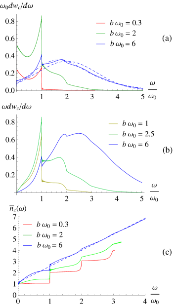
Figure 6: (a) Multiphoton probability spectra computed for dipole harmonic coherent radiation defined through Eqs. (57–58) (solid curves). Red curve, corresponding to intensity parameter $b\omega_{0}=0.3$, $\bar{n}=\frac{2}{3}b\omega_{0}=0.2$ [small deviations from the single-photon spectrum (58)]. Green curve, the same for $b\omega_{0}=2$ (the highest summit reached by the fundamental maximum). Blue curves, $b\omega_{0}=6$ (onset of high-intensity regime). Dashed blue curve, Gaussian approximation (113). Dot-dashed blue curve, corrected Gaussian approximation (120). (b) Multiphoton energy spectrum $\omega\frac{dw_{\text{c}}}{d\omega}$ for the same single-photon spectrum as in (a), and intensity parameter values $b\omega_{0}=1$, 2.5, 6. The development of secondary maxima for the energy spectrum is more spectacular than for the probability spectrum $\frac{dw_{\text{c}}}{d\omega}$. (c) Photon multiplicity spectrum described by Eqs. (39), (57–58). Solid curves correspond to same parameters as in (a). Dashed blue line is high-intensity approximation (117).

Inserting entries (57–58) to Mellin integrals (17) and (39), and computing them numerically, one can trace the evolution of the resummed spectrum and the multiplicity spectrum with the increase of the intensity. This is illustrated in Fig. 6 for a few values of $b\omega_{0}$. The trends observed in those figures are: smoothening of the spectral shape with the increase of the intensity, the existence of an upper bound for the probability distribution (Fig. 6a), the appearance of a second maximum in the energy spectrum at moderate intensity (Fig. 6b, green curve), and monotonic increase of the photon multiplicity spectrum with $\omega$ (Fig. 6c). Explaining the origin of those features will occupy us next.

III.2.1 Multiphoton coherent radiation spectrum in the fundamental energy interval

When the single-photon spectrum is described by Eq. (57), at sufficiently low radiation intensity, the multiphoton spectrum will as well be concentrated within the interval $0\leq\omega<\omega_{0}$ (termed fundamental) – see Fig. 6a, red and green curves. So, it seems natural to begin with evaluation of the multiphoton spectrum in the fundamental interval.

The calculation is straightforward based on representation (17), written for finite $w_{1\text{c}}$ as

$$\frac{dw_{\text{c}}}{d\omega}=e^{-w_{1\text{c}}}\frac{1}{2\pi i}\int_{c-i\infty}^{c+i\infty}\!dse^{s\omega+b\!\int_{0}^{\infty}d\omega_{1}P(\omega_{1}/\omega_{0})e^{-s\omega_{1}}}\quad$$ (60)

$$(0<\omega<\omega_{0}).\qquad\qquad\qquad\qquad$$

Here we dropped the $\delta$-term for $\omega>0$, and by virtue of Lemma 1, the upper limit in the integral over $\omega_{1}$ was replaced by infinity, without the necessity to employ the Heaviside step function, which therefore was omitted. If $P$ is a polynomial, like (58), the integral in the exponent of (60) evaluates as a finite-order polynomial in $s^{-1}$:

$$\int_{0}^{\infty}d\omega_{1}P\left(\frac{\omega_{1}}{\omega_{0}}\right)e^{-s\omega_{1}}=\sum_{k=0}^{2}\frac{P^{(k)}(0)}{s^{1+k}\omega_{0}^{k}},$$ (61)

where $P^{(k)}$ stands for the $k$-th derivative of $P(z)$ w.r.t. its argument. Inserting (61) to (60), and rescaling the integration variable to $s=\zeta/\omega_{0}$, yields

$$\frac{dw_{\text{c}}}{d\omega}=\frac{e^{-w_{1\text{c}}}}{\omega_{0}}\frac{1}{2\pi i}\oint_{\mathcal{C}_{3}}d\zeta e^{\zeta\frac{\omega}{\omega_{0}}+b\omega_{0}\sum_{k=0}^{2}\frac{P^{(k)}(0)}{\zeta^{1+k}}}$$ (62)

$$(0<\omega<\omega_{0}).\qquad\qquad$$

Benefiting from the exponential decrease of the integrand at $\mathfrak{Re}\zeta\to-\infty$, along with the absence of cuts in the complex $\zeta$-plane, we replaced the infinite integration contour by a closed loop encircling the origin, where the only singularity of the integrand resides (contour $\mathcal{C}_{3}$ in Fig. 4).

Infrared limit.

Despite the closed integration contour, and representation of the exponent in the integrand by only a few power terms, integral (62) generally does not permit classification in terms of basic special functions. But it is instructive at least to obtain its expansion about endpoint $\omega=+0$. There, one of the exponentials tends to unity, $e^{\zeta\frac{\omega}{\omega_{0}}}\to 1$, and if the second exponential is expanded into Laurent series

$$e^{b\omega_{0}\sum_{k=0}^{2}\frac{P^{(k)}(0)}{\zeta^{1+k}}}=\sum_{m=0}^{\infty}\frac{c_{m}}{\zeta^{m}},$$ (63)

the only term surviving after the loop integration is $\frac{c_{1}}{\zeta}=b\omega_{0}P(0)\frac{1}{\zeta}$, leaving the result

$$\frac{dw_{\text{c}}}{d\omega}\bigg{|}_{\omega=+0}=bP(0)e^{-w_{1\text{c}}}\equiv e^{-w_{1\text{c}}}\frac{dw_{1\text{c}}}{d\omega_{1}}\bigg{|}_{\omega_{1}=+0}.$$ (64)

This equation shows that in the limit $\omega\to 0$, the single-photon probability dominates, albeit in conjunction with photon non-emission probability $e^{-w_{1\text{c}}}$. For the photon multiplicity spectrum, Eq. (64), when inserted to Eq. (40) leads to Eq. (38).

To derive an $\mathcal{O}(\omega)$ correction to Eq. (64), one needs to retain also a linear term in the expansion of $e^{\zeta\frac{\omega}{\omega_{0}}}$:

$$\frac{dw_{\text{c}}}{d\omega}=e^{-w_{1\text{c}}}b\left\{\!P(0)\!+\!\frac{\omega}{\omega_{0}}\!\left[P^{\prime}(0)\!+\!\frac{b\omega_{0}}{2}P^{2}(0)\right]\!\!+\!\mathcal{O}(\omega^{2})\!\right\}\!.$$ (65)

For our specific example (58), $P^{\prime}(0)=-2<0$. But for a sufficiently high intensity, specifically

$$b\omega_{0}>-\frac{2P^{\prime}(0)}{P^{2}(0)}=4,$$ (66)

the coefficient at the linear term in (65) turns positive, wherewith the resummed spectrum in the whole fundamental interval becomes monotonously increasing. That may be associated with the inception of high-intensity regime, which will be examined in the next section.

From Eqs. (65) and (40), one similarly infers an expression for the photon multiplicity spectrum

$$\bar{n}_{\text{c}}(\omega)=1+\frac{bP(0)}{2}\omega+\mathcal{O}(\omega^{2}).$$ (67)

This shows that the slope in the origin does not depend on $P^{\prime}(0)$, and is always positive, in accord with Eq. (37). The increase of the slope in the origin with the increase of parameter $b$ agrees with Fig. 6b.

Fundamental maximum.

The opposite endpoint of the fundamental interval, $\omega=\omega_{0}-0$, is of prime practical significance, as long as it represents the global spectral maximum at moderate radiation intensity. Substituting $\omega=\omega_{0}$ in Eq. (62) leaves

$$\omega_{0}\frac{dw_{\text{c}}}{d\omega}\bigg{|}_{\omega=\omega_{0}-0}=e^{-w_{1\text{c}}}\frac{1}{2\pi i}\oint_{\mathcal{C}_{3}}d\zeta e^{\zeta+b\omega_{0}\sum_{k=0}^{2}\frac{P^{(k)}(0)}{\zeta^{1+k}}}.$$ (68)

Effectively, this is a function of a single dimensionless parameter $b\omega_{0}$, inasmuch as all $P^{(k)}(0)\sim 1$. In Fig. 7, the dependence of (68) on $b\omega_{0}$ [with $P(z)$ defined by Eq. (58)] is displayed by the solid gray curve. Naturally, with the increase of $b$, at first it rises proportionally, but eventually the rise halts and ends up with a decrease, formally owing to factor $e^{-w_{1\text{c}}}$. The ultimate suppression of the resumed spectrum at any fixed energy $\omega$ is not surprising, given the saturation of total probability (10) on one hand, and the spread of the spectrum to higher $\omega$ on the other hand.

To estimate the maximal summit of function (68), one can adopt the following approach. To capture the first bend of the nonlinear $b$-dependence, expand the contour integral in (68) to second order in $b$ (which is equivalent to keeping in Eq. (9) the first two terms):

$$\omega_{0}\frac{dw_{\text{c}}}{d\omega}\bigg{|}_{\omega=\omega_{0}-0} \simeq e^{-w_{1\text{c}}}\bigg{[}b\omega_{0}\sum_{k=0}^{2}\frac{P^{(k)}(0)}{k!}\qquad$$ (69)

$$+\frac{b^{2}\omega_{0}^{2}}{2}\sum_{k,l=0}^{2}\frac{P^{(k)}(0)P^{(l)}(0)}{(k+l+1)!}\bigg{]}$$

$$= P(1)e^{-b\omega_{0}\xi}\left(b\omega_{0}+\frac{b^{2}\omega_{0}^{2}}{2}\eta\right),\,\,$$

where

$$\xi=\int_{0}^{1}dzP(z),$$ (70)

$$\eta=\frac{1}{P(1)}\int_{0}^{1}dzP(z)P(1-z).$$ (71)

The behavior of approximation (69) is illustrated in Fig. 7 by the dashed gray curve. The maximum of (69) can be explicitly found by differentiation by $b\omega_{0}$: it is situated at

$$b_{\star}\omega_{0}=\frac{1}{\xi}-\frac{1}{\eta}+\sqrt{\frac{1}{\xi^{2}}+\frac{1}{\eta^{2}}}.$$ (72)

For $P(z)$ described by Eq. (58) (wherewith $\xi=\frac{2}{3}$, $\eta=\frac{7}{15}$), Eq. (72) yields $b_{\star}\omega_{0}\approx 2.0$, at which $\omega_{0}\frac{dw_{\text{c}}}{d\omega}\big{|}_{\omega=\omega_{0}-0}=0.77$. For comparison, the maximum of exact expression (68) is achieved at $b\omega_{0}\approx 2.26$, and amounts 0.84 (see Fig. 7, solid gray curve). Hence, at any radiation intensity, the probability spectrum $\frac{dw}{d\omega}$ of multiphoton coherent radiation at practice never exceeds unity – in marked contrast with the unlimited growth of the single-photon spectrum. [At that, the energy spectrum $\omega\frac{dw}{d\omega}$ can indefinitely grow, $\sim\sqrt{b}$ – see Sec. IV.2.2, Eq. (113)].

Figure 7: The spectral intensity at the fundamental maximum ($\omega=\omega_{0}-0$) vs. the radiator length (in units of $b\omega_{0}$), for a single-photon spectrum described by Eq. (58). Solid gray curve, pure coherent radiation [Eq. (68)]. Dashed gray curve, approximation (69). Solid black curve, the combination of coherent and incoherent radiation [Eq. (84)] in proportion $a=b\omega_{0}/20$, for $E=10\,\omega_{0}$ ($E_{e}\approx 20\,\omega_{0}$). Dashed black curve, approximation (III.3.2).

III.2.2 Discontinuity at $\omega=\omega_{0}$

Besides peaking at $\omega=\omega_{0}$, the coherent radiation spectrum encounters at this point a discontinuity, which is actually easier to evaluate. For our simplified case (58), the discontinuity of the single-photon spectrum (defined to be a positive quantity) just equals the height of its maximum:

$$\Delta_{1\text{c}}|_{\omega_{0}}=\frac{dw_{1\text{c}}}{d\omega_{1}}\bigg{|}_{\omega_{1}=\omega_{0}-0}-\frac{dw_{1\text{c}}}{d\omega_{1}}\bigg{|}_{\omega_{1}=\omega_{0}+0}=bP(1).$$ (73)

With the account of emission of several photons, the spectrum beyond $\omega_{0}$ deviates from zero, so higher terms of series (9) demand consideration. But all terms with $n\geq 2$ prove to be continuous. Hence, the discontinuity of the total spectrum just equals that of the first term. This term yet involves the total photon non-emission probability factor

$$\Delta_{\text{c}}|_{\omega_{0}}=\Delta_{1\text{c}}|_{\omega_{0}}e^{-w_{1\text{c}}}=bP(1)e^{-b\omega_{0}\int_{0}^{1}dzP(z)},$$ (74)

which embodies all the multiphoton effects on the discontinuity.

At multiples of the fundamental energy, $\omega=n\omega_{0}$ with integer $n\geq 2$, the resummed spectrum remains continuous, but its $(n-1)$-th derivative encounters a discontinuity (as can be noticed already from Figs. 6). That also follows from the analysis of the phase space available for integration for terms of series (9a,b). Furthermore, even in case if function $P(z)$ is vanishing at $z\to 1$, in representation (9) the function discontinuity at $\omega=\omega_{0}$ cancels, but discontinuities of its derivatives persist. We leave the proof of those statements to the reader.

As regards the discontinuities of $\bar{n}_{\text{c}}(\omega)$, Fig. 6c shows that they are similar to those of $\frac{dw_{\text{c}}}{d\omega}$, but have opposite sign [because $\bar{n}_{\text{c}}(\omega)$ contains $dw/d\omega$ in the denominator]. At low radiation intensity, the multiplicity spectrum exhibits a step-like behavior, approximately amounting to the smallest integer greater than $\omega/\omega_{0}$. That is traced to the fact that in an interval $n-1<\omega/\omega_{0}<n$ $(n\in\mathbb{N})$, the $n$-photon component dominates. As the intensity increases, function $\bar{n}_{\text{c}}(\omega)$ smoothens out, given that a $n$-photon component becomes competitive with fewer-photon components even in intervals where those components are not yet extinct.

III.3 Combination of coherent and incoherent radiation

Having explored separately the shapes of resummed coherent and incoherent radiation spectra, we are now in a position to examine their nonlinear interplay. The physical example when those components are both significant is coherent bremsstrahlung, occurring when an electron or positron crosses a family of crystalline planes at an above-critical (although small) angle. Thereat, the continuous interplanar potential acts on the electron periodically, evoking coherent radiation books-on-coh-sources ; Ter-Mik ; Diambrini-Palazzi . At the same time, the incoherent scattering on atomic nuclei in the planes causes incoherent bremsstrahlung, similar to that in amorphous matter. In a satisfactory approximation, the single-photon radiation spectrum may be expressed as a sum of two non-interfering parts:

$$\frac{dw_{1}}{d\omega_{1}}=\frac{dw_{1\text{i}}}{d\omega_{1}}+\frac{dw_{1\text{c}}}{d\omega_{1}},$$ (75)

where $\frac{dw_{1\text{i}}}{d\omega_{1}}$ is given by Eq. (42). In graphical illustrations, we will continue using Eqs. (57–58) for $\frac{dw_{1\text{c}}}{d\omega_{1}}$, i.e., neglect higher harmonics. In some cases, those can be small indeed even for coherent bremsstrahlung (‘one-point’ spectra, see Diambrini-Palazzi ). At the same time, we saw in the previous section that the second maximum in the multiphoton spectrum can be generated even in the absence of secondary harmonics in the single-photon spectrum, so it will be expedient to check whether their effect is anyhow affected by incoherent radiation.

For what concerns the ratio of magnitudes of coherent and incoherent radiation components, for coherent bremsstrahlung it obeys a relation

$$\frac{a}{b\omega_{0}}\simeq C\chi\qquad(\text{coh. bremsstr.}),$$ (76)

with $\chi$ the misalignment angle between the electron momentum and the co-oriented family of atomic planes, and $C\sim 10$ [cf. Eqs. (43) and (173)]. At typical $\chi\sim 10^{-2}\div 10^{-4}$, ratio (76) is pretty small. Nevertheless, effects of incoherent radiation in the spectrum may be quite noticeable. That is illustrated by Fig. 8, where in spite of rather large initial ratio $b\omega_{0}/a=20$, the incoherent bremsstrahlung plateau in the multiphoton energy spectrum $\omega\frac{dw}{d\omega}$ is only a few times lower than the spectrum height in the maximum (Fig. 8b). Handling the effects of incoherent radiation proves to be most convenient with the aid of a convolution representation derived below.

III.3.1 Convolution representations

Once decomposition (75) is inserted to Eq. (17), the exponential in the integrand splits into a product of two factors, one depending on $\frac{dw_{1\text{i}}}{d\omega}$, and the other on $\frac{dw_{1\text{c}}}{d\omega}$. Expressing then each of those factors via Eq. (15) through Laplace transforms of the corresponding resummed radiation spectra, and doing the contour integral, we arrive at a convolution relation:

$$\frac{dw}{d\omega}=\int_{0}^{\omega}d\omega^{\prime}\frac{dw_{\text{i}}}{d\omega^{\prime}}\frac{dw_{\text{c}}}{d\omega^{\prime\prime}}\bigg{|}_{\omega^{\prime\prime}=\omega-\omega^{\prime}}+e^{-w_{1\text{c}}}\frac{dw_{\text{i}}}{d\omega}$$ (77)

$$+\underset{\hookrightarrow 0}{e^{-w_{1\text{i}}}}\frac{dw_{\text{c}}}{d\omega}.$$

The term in the second line vanishes if $w_{1\text{i}}$ diverges, whereupon expression (77) becomes linear in $dw_{\text{i}}$. Still, the resulting convolution is non-vanishing at $a\to 0$, because, as we saw in Sec. III.1, the multiphoton incoherent radiation spectrum in this limit tends to a $\delta$-function, not to zero [see Eq. (53)]. More precisely, if median $\omega_{\text{i}\frac{1}{2}}$ defined by Eq. (54) proves to be much smaller than $\omega_{0}$, convolution (77) will be close to $\frac{dw_{\text{c}}}{d\omega}$.

Observing further that in Eq. (77) $\frac{dw_{\text{i}}}{d\omega^{\prime}}$ is a smooth function, whereas the coherent radiation spectrum $\frac{dw_{\text{c}}}{d\omega^{\prime\prime}}\big{|}_{\omega^{\prime\prime}=\omega-\omega^{\prime}}$ is not, it may be beneficial to integrate in (77) by parts:

$$\frac{dw}{d\omega}=e^{-w_{1\text{c}}}\frac{dw_{\text{i}}}{d\omega}+\frac{dw_{\text{c}}}{d\omega^{\prime\prime}}\bigg{|}_{\omega^{\prime\prime}=0}\int_{0}^{\omega}d\omega^{\prime\prime\prime}\frac{dw_{\text{i}}}{d\omega^{\prime\prime\prime}}\qquad\qquad$$

$$-\int_{0}^{\omega}d\omega^{\prime}\left(\int_{0}^{\omega^{\prime}}d\omega^{\prime\prime\prime}\frac{dw_{\text{i}}}{d\omega^{\prime\prime\prime}}\right)\!\frac{d}{d\omega^{\prime}}\!\left(\frac{dw_{\text{c}}}{d\omega^{\prime\prime}}\bigg{|}_{\omega^{\prime\prime}=\omega-\omega^{\prime}}\right)\!.\quad$$ (78)

Invoking here Eq. (64) along with identity $\int_{0}^{\omega}d\omega^{\prime\prime\prime}\frac{dw_{\text{i}}}{d\omega^{\prime\prime\prime}}=\Phi(a)\left(\frac{\omega}{E}\right)^{a}$, the convolution relation recasts

$$\frac{dw}{d\omega}=e^{-w_{1\text{c}}}\Phi(a)\left(\frac{\omega}{E}\right)^{a}\left[\frac{a}{\omega}+bP(0)\right]\qquad\qquad\quad$$

$$-\Phi(a)\int_{0}^{\omega}d\omega^{\prime}\left(\frac{\omega^{\prime}}{E}\right)^{a}\frac{d}{d\omega^{\prime}}\left(\frac{dw_{\text{c}}}{d\omega^{\prime\prime}}\bigg{|}_{\omega^{\prime\prime}=\omega-\omega^{\prime}}\right).$$ (79)

The merit of the latter representation is that it picks up discrete contributions from points at which $\frac{dw_{\text{c}}}{d\omega^{\prime\prime}}\big{|}_{\omega^{\prime\prime}=\omega-\omega^{\prime}}$ encounters discontinuities, transforming to $\delta$-function-like terms for its derivative.

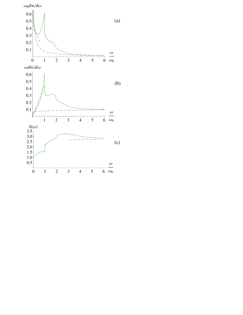
Figure 8: (a) Multiphoton radiation spectrum involving coherent component with magnitude $b\omega_{0}=2$, and incoherent component with $a=0.1$. The UV cutoff parameter is chosen at $E=10\,\omega_{0}$. Solid green curve, the exact result obtained by numerical evaluation of the contour integral. Long-dashed black curve, corrected low-$\omega$ approximation (III.3.2). Dotted black curve, approximation next to the coherent emission edge, Eq. (87). Dot-dashed black curve, large-$\omega$ asymptotics (89). (b) The energy spectrum for same conditions as in (a). Short-dashed black curve, low-$\omega$ approximation (80). Dot-dashed black curve, large-$\omega$ asymptotics (89). (c) The photon multiplicity spectrum for same parameters as in (a,b), and IR cutoff $\epsilon=0.1\,\omega_{0}$. Solid green curve, exact result. Dot-dashed black curve, large-$\omega$ approximation (91).

In the limit $\omega\to 0$, the integral term in Eq. (III.3.1), vanishes due to the integration interval shrinkage, leaving

$$\frac{dw}{d\omega}=e^{-w_{1\text{c}}}\Phi(a)\left(\frac{\omega}{E}\right)^{a}\left[\frac{a}{\omega}+bP(0)+\mathcal{O}(\omega)\right].$$ (80)

Clearly, here the leading term $\frac{a}{\omega}$ represents the contribution due to incoherent bremsstrahlung, but it receives an extra suppression by factor $e^{-w_{1\text{c}}}$ depending on the coherent radiation. Hence, the incoherent component can not be asserted to dominate in this limit alone, in contrast to the case of large $\omega$ (see Sec. III.3.4 below). The behavior of asymptotic approximation (80) is illustrated in Fig. 8b by the short-dashed black curve.

In a similar fashion, one can derive a convolution relation for the multiplicity spectrum, which reads

$$\bar{n}(\omega)\frac{dw}{d\omega}=\int_{0}^{\omega}d\omega^{\prime}\frac{dw_{\text{c}}}{d\omega^{\prime}}\frac{dw_{\text{i}}}{d\omega^{\prime\prime}}\bigg{|}_{\omega^{\prime\prime}=\omega-\omega^{\prime}}\qquad\qquad$$

$$\times\left[\bar{n}_{\text{c}}(\omega^{\prime})+\bar{n}_{\text{i}}(\omega-\omega^{\prime})\right]$$ (81)

$$+e^{-w_{1\text{c}}}\bar{n}_{\text{i}}(\omega)\frac{dw_{\text{i}}}{d\omega}+\underset{\hookrightarrow 0}{e^{-w_{1\text{i}}}}\bar{n}_{\text{c}}(\omega)\frac{dw_{\text{c}}}{d\omega},$$

with $\bar{n}_{\text{c}}(\omega)$ and $\bar{n}_{\text{i}}(\omega)$ the corresponding multiplicity spectra for pure coherent and incoherent components. In particular, from Eqs. (III.3.1) and (77) one observes that both $\frac{dw}{d\omega}$, and $\frac{dw_{\text{i}}}{d\omega}$ involve $E$-dependent factors $E^{-a}$, which cancel between l.h.s. and r.h.s. of Eq. (III.3.1). Thus, $\bar{n}(\omega)$ is independent of $E$, as anticipated.

III.3.2 Spectrum of combined radiation in the fundamental interval

For an efficient coherent radiator, the coherent spectral component must prevail in the fundamental interval $0<\omega\leq\omega_{0}$, anyway. It is thus instructive to repeat the analysis of Sec. III.2.1 for a mixture of coherent and incoherent radiation components in the fundamental interval. We will barely sketch it here, emphasizing the distinctions from the pure coherent radiation case.

Once expressions (75), (42), (57) are inserted to Eq. (II.2), manipulations similar to those used at derivation of Eq. (62) yield

$$\frac{dw}{d\omega}\!=\!\frac{e^{-\gamma_{\text{E}}a-w_{1\text{c}}}}{\omega_{0}}\!\left(\frac{\omega_{0}}{E}\right)^{\!a}\!\frac{1}{2\pi i}\!\int_{\mathcal{C}_{2}}\!\frac{d\zeta}{\zeta^{a}}e^{\zeta\!\frac{\omega}{\omega_{0}}+b\omega_{0}\!\sum_{k=0}^{2}\!\!\frac{P^{(k)}\!(0)}{\zeta^{1+k}}}\quad$$ (82)

$$(\omega<\omega_{0}).\qquad\qquad\qquad\qquad$$

Here exponential decrease of the integrand at $\mathfrak{Re}\zeta\to-\infty$ justifies deformation of the integration contour to shape $\mathcal{C}_{2}$ (see Fig. 4), but its complete enclosure is impossible because of the presence of branching factor $\zeta^{-a}$.

Infrared limit.

When $\omega\to+0$, contour integral (82) is dominated by large $\zeta$. Then, the leading-order term in asymptotic expansion (63) reproduces result (80). Retaining next-to-leading order terms yields an $\mathcal{O}(\omega)$ correction:

$$\frac{dw}{d\omega}=e^{-w_{1\text{c}}}\Phi(a)\left(\frac{\omega}{E}\right)^{a}\Bigg{\{}\frac{a}{\omega}+bP(0)\qquad\qquad\quad$$

$$+\frac{b\omega}{(1+a)\omega_{0}}\left[P^{\prime}(0)+\frac{b\omega_{0}}{2}P^{2}(0)\right]+\mathcal{O}(\omega^{2})\Bigg{\}}.$$ (83)

Compared to (65), apart from the overall factor $\left(\frac{\omega}{E}\right)^{a}$, there emerges a term $\frac{a}{\omega}$, whereas other terms remain essentially the same. The term in the second line of Eq. (III.3.2) changes its sign under the same condition (66), so inception of high-intensity regime is essentially independent of $a$. The behavior of asymptotic approximation (III.3.2) is illustrated in Fig. 8a by the gray long-dashed curve.

Reduction of the fundamental maximum by hard incoherent bremsstrahlung.

In the point of the spectral fundamental maximum, $\omega\to\omega_{0}-0$, integral (82) reduces to

$$\frac{dw}{d\omega}\bigg{|}_{\omega=\omega_{0}-0} = \frac{e^{-\gamma_{\text{E}}a-w_{1\text{c}}}}{\omega_{0}}\left(\frac{\omega_{0}}{E}\right)^{a}$$ (84)

$$\times\frac{1}{2\pi i}\int_{\mathcal{C}_{2}}\frac{d\zeta}{\zeta^{a}}e^{\zeta+b\omega_{0}\sum_{k=0}^{2}\frac{P^{(k)}(0)}{\zeta^{1+k}}}.\qquad$$

Since $a$ and $b$ are both proportional to the target thickness, the increase of the latter at fixed $\chi$ [cf. Eq. (76)] corresponds to a simultaneous increase of $b$ and $a$, at ratio $a/b$ held fixed. For an exemplary ratio $a/b=\omega_{0}/20$, the spectral intensity in the fundamental maximum is illustrated in Fig. 7 by solid gray curve. Compared to the pure coherent radiation spectrum, its maximum is achieved at a slightly lower value of $b$, and its height is somewhat lower, too. This owes primarily to factor $\left(\frac{\omega_{0}}{E}\right)^{a}$, where $\frac{\omega_{0}}{E}$ is a small number, but there can also be other appreciable effects of $a$.

To assess changes in the height and location of the fundamental maximum due to incoherent radiation, one can, as in Sec. III.2.1, expand the contour integral in (84) to second order in $b$ and $a$:

$$\frac{dw}{d\omega}\bigg{|}_{\omega=\omega_{0}-0}\approx e^{-w_{1\text{c}}}\left(1-\gamma_{\text{E}}a-a\ln\frac{E}{\omega_{0}}\right)\Bigg{[}\frac{1}{\omega_{0}\Gamma(a)}\quad\qquad$$

$$+b\sum_{k=0}^{2}\frac{P^{(k)}(0)}{\Gamma(k+1+a)}+\frac{b^{2}\omega_{0}}{2}\sum_{k,l=0}^{2}\frac{P^{(k)}(0)P^{(l)}(0)}{\Gamma(k+l+2+a)}\Bigg{]}.$$

It may suffice to account for corrections in $a$ within the leading logarithmic accuracy, which gives

$$\frac{dw}{d\omega}\bigg{|}_{\omega=\omega_{0}-0}\approx e^{-w_{1\text{c}}}\Bigg{\{}\!\!\left(1-a\ln\frac{E_{e}}{\omega_{0}}\right)\!\left[\frac{a}{\omega_{0}}+bP(1)\right]\,\,\,$$

$$+\frac{b^{2}\omega_{0}}{2}\int_{0}^{1}dzP(z)P(1-z)\Bigg{\}}\quad$$ (85)

(see Fig. 7, dashed black curve). Here term $-a\ln\frac{E_{e}}{\omega_{0}}$ can be sizable due to the large logarithm, despite the condition $a\ll 1$. Owing to its negative sign, that correction reduces the height of the fundamental coherent radiation maximum, in addition to factor $e^{-w_{1\text{c}}}$.

In the spirit of Sec. III.2.1, for approximation (III.3.2) one can determine the target thickness at which the spectral radiation intensity in the fundamental maximum reaches its highest summit. It is still given by formula (72), with parameter $\xi$ unaltered, but parameter $\eta$ modifies to

$$\eta=\frac{\int_{0}^{1}dzP(z)P(1-z)-\frac{2a}{b\omega_{0}}\ln\frac{E_{e}}{\omega_{0}}}{P(1)+\frac{a}{b\omega_{0}}}.$$ (86)

Corrections in the numerator and denominator of (86) both result in lowering of $\eta$, and therethrough in an earlier turnover of the fundamental maximum, as confirmed by Fig. 7. The largest effect, of course, stems from the logarithmic term in (86).

III.3.3 Regulation of spectrum discontinuities by soft incoherent bremsstrahlung

A principally interesting effect of incoherent radiation concerns discontinuities of the coherent radiation spectrum. As we saw in Sec. III.2.2, the discontinuity at $\omega=\omega_{0}$ is damped by factor $e^{-w_{\text{c}}}$. With the addition of the incoherent bremsstrahlung component, this factor actually turns to zero, wherefore the discontinuity must be nullified. Our analysis of the spectrum behavior then needs extension to a non-vanishing vicinity of point $\omega=\omega_{0}$.

In vicinity of a singularity of the coherent part of the spectrum, it is convenient to use representation (III.3.1). When $\omega$ slightly exceeds $\omega_{0}$, the integrand of (III.3.1) receives an extra contribution proportional to a $\delta$-function

$$\frac{d}{d\omega^{\prime}}\left(\frac{dw_{\text{c}}}{d\omega^{\prime\prime}}\bigg{|}_{\omega^{\prime\prime}=\omega-\omega^{\prime}}\right)\underset{\omega^{\prime}\approx\omega-\omega_{0}}{\simeq}-\Delta_{\text{c}}|_{\omega_{0}}\delta(\omega-\omega_{0}-\omega^{\prime}),$$

where $\Delta_{\text{c}}|_{\omega_{0}}$ is given by Eq. (74). Integration of the $\delta$-singularity yields a sizable contribution even at an infinitesimal extension of $\omega$ beyond $\omega_{0}$:

$$\frac{dw}{d\omega}\simeq\frac{dw}{d\omega^{\prime}}\bigg{|}_{\omega^{\prime}=\omega_{0}}-\Delta_{\text{c}}|_{\omega_{0}}\!\left(\frac{\omega-\omega_{0}}{E}\right)^{\!a}\theta(\omega-\omega_{0})+\mathcal{O}(\omega-\omega_{0}).$$ (87)

Eq. (87) shows that for $a>0$, factor $\left(\frac{\omega-\omega_{0}}{E}\right)^{a}$ vanishes as $\omega\to\omega_{0}+0$, indeed nullifying the discontinuity brought by factor $\theta(\omega-\omega_{0})$, and making the whole spectrum everywhere continuous. But the derivative of factor $\left(\frac{\omega-\omega_{0}}{E}\right)^{a}$ in point $\omega=\omega_{0}$ diverges, wherewith the resulting spectrum features a sharp spike. The behavior of approximation (87) is shown in Fig. 8a by the dotted black curve.

It should be realized, though, that the described subtle effect should be obscured in experiments with limited energy resolution and finite angular divergence of the initial beam, which smear the fundamental peak. Besides that, the filling of the dip adjacent to the coherent radiation maximum is also partially provided by the pure coherent multiphoton spectrum, whose derivative beyond $\omega_{0}$ is negative (see Fig. 6a). Thus, verification of threshold behavior (87) may be feasible only with a rather perfect beam, and in a sufficiently thick target, when $a$ becomes sizable.

III.3.4 Large-$\omega$ asymptotics

To accomplish our analysis in different regions, let us consider the large-$\omega$ asymptotics $\overline{\omega_{1}}_{\text{c}},\omega_{0}\ll\omega$ (while still obeying condition $\omega\ll E$). In this limit, the incoherent bremsstrahlung spectrum decreases by a power law, whereas the multiphoton coherent radiation spectrum, in general, decreases exponentially (see Appendix C). Therefore, if Eq. (77) is rewritten as

$$\frac{dw}{d\omega}=\int_{0}^{\omega}d\omega^{\prime}\frac{dw_{\text{c}}}{d\omega^{\prime}}\frac{dw_{\text{i}}}{d\omega^{\prime\prime}}\bigg{|}_{\omega^{\prime\prime}=\omega-\omega^{\prime}}+e^{-w_{1\text{c}}}\frac{dw_{\text{i}}}{d\omega},$$

the main contribution to the integral over $\omega^{\prime}$ comes from vicinity of the lower integration limit. Thus, we can expand $\frac{dw_{\text{i}}}{d\omega^{\prime\prime}}$ to Taylor series about point $\omega^{\prime\prime}=\omega-\overline{\omega_{1\!}}_{\text{c}}$, and replace the upper integration limit by infinity:

$$\frac{dw}{d\omega} = \frac{dw_{\text{i}}}{d\omega^{\prime\prime}}\bigg{|}_{\omega^{\prime\prime}=\omega-\overline{\omega_{1\!}}_{\text{c}}}\int_{0}^{\infty}d\omega^{\prime}\frac{dw_{\text{c}}}{d\omega^{\prime}}$$

$$+\frac{d}{d\omega^{\prime\prime}}\frac{dw_{\text{i}}}{d\omega^{\prime\prime}}\bigg{|}_{\omega^{\prime\prime}=\omega-\overline{\omega_{1\!}}_{\text{c}}}\int_{0}^{\infty}d\omega^{\prime}\frac{dw_{\text{c}}}{d\omega^{\prime}}\left(\overline{\omega_{1\!}}_{\text{c}}-\omega^{\prime}\right)+\ldots$$

$$\qquad\qquad\qquad\qquad\qquad+e^{-w_{1\text{c}}}\frac{dw_{\text{i}}}{d\omega}.$$

The integral in the second line vanishes due to Eq. (30), leaving

$$\frac{dw}{d\omega}=\frac{a\Phi(a)}{E^{a}}\Bigg{[}\frac{1-e^{-w_{1\text{c}}}}{(\omega-\overline{\omega_{1\!}}_{\text{c}})^{1-a}}+\frac{e^{-w_{1\text{c}}}}{\omega^{1-a}}+\mathcal{O}\!\left(\!\frac{\overline{\omega^{2}_{1\!}}_{\text{c}}}{(\omega-\overline{\omega_{1\!}}_{\text{c}})^{3-a}}\!\right)\!\!\Bigg{]}.$$ (88)

Furthermore, in the limit $\omega\gg\overline{\omega_{1\!}}_{\text{c}}$, Eq. (88) boils down to

$$\frac{dw}{d\omega}\simeq\frac{dw_{\text{i}}}{d\omega}\left[1+\mathcal{O}\left(\frac{\overline{\omega_{1\!}}_{\text{c}}}{\omega}\right)\right],$$ (89)

which is shown in Figs. 8a,b by dot-dashed black curves. Eq. (89) implies that the combined spectrum ultimately decreases by the same power law as its (resummed) incoherent bremsstrahlung component. That property is in contrast with the infrared limit (80), which yet involves factor $e^{-w_{1\text{c}}}$ of coherent photon non-emission probability [note the difference between green and black long-dashed curves in Fig. 8a at small $\omega$].

Finally, it is straightforward to derive large-$\omega$ asymptotics for the photon multiplicity spectrum, with the aid of Eq. (III.3.1). Due to factor $\frac{dw_{\text{c}}}{d\omega^{\prime}}$ in the integrand of (III.3.1), again, the dominant contribution comes from the lower integration limit, where it is acceptable to replace $\frac{dw_{\text{i}}}{d\omega^{\prime\prime}}\big{|}_{\omega^{\prime\prime}=\omega-\omega^{\prime}}=\frac{dw_{\text{i}}}{d\omega}\left[1+\mathcal{O}\left(\frac{\omega^{\prime}}{\omega}\right)\right]$, $\bar{n}_{\text{i}}(\omega-\omega^{\prime})=\bar{n}_{\text{i}}(\omega)\left[1+\mathcal{O}\left(\frac{a\omega^{\prime}}{\omega}\right)\right]$, and replace the upper integration limit by infinity. Therewith, Eq. (III.3.1) yields

$$\bar{n}(\omega)\frac{dw}{d\omega}\approx\frac{dw_{\text{i}}}{d\omega}\left[\bar{n}_{\text{i}}(\omega)+\int_{0}^{\infty}d\omega^{\prime}\frac{dw_{\text{c}}}{d\omega^{\prime}}\bar{n}_{\text{c}}(\omega^{\prime})\right],$$ (90)

where $\bar{n}_{\text{i}}(\omega)$ is given by Eq. (55). (Terms involving $e^{-w_{1\text{c}}}$ canceled mutually.) The integral entering (90) equals $w_{1\text{c}}=\bar{n}_{\text{c}}$, as can be checked with the aid of Eq. (39). Canceling in (90) the overall factors according to Eq. (89), we are left with

$$\bar{n}(\omega)=\left[\bar{n}_{\text{c}}+\bar{n}_{\text{i}}(\omega)\right]\left[1+\mathcal{O}\left(\frac{\overline{\omega_{1\!}}_{\text{c}}}{\omega}\right)\right].$$ (91)

The behavior of the photon multiplicity spectrum is shown in Fig. 8c by the solid green curve. At large $\omega$, it flattens out, and ultimately enters the regime of logarithmic growth as predicted by Eq. (91) (dot-dashed black curve). Yet before entering the asymptotic regime, as Fig. 8b shows, the multiplicity spectrum first achieves a maximum, then passes through a shallow minimum. The theory for such a behavior will be provided in Sec. IV.3.

III.4 Identification of multiphoton effects against other effects in measured spectra

The preceding analysis revealed that multiphoton emission effects redistribute the coherent radiation spectrum, elevating it beyond the fundamental energy $\omega_{0}$, at the expense of reduction below $\omega_{0}$. At practice, though, one should yet be aware of existence of other physical processes which can produce superficially similar effects. In conclusion of this section, we will briefly discuss such effects, too.

First of all, next to the coherent emission edge $\omega_{0}$, the spectrum may receive an enhancement not only from multiphoton effects, but also from higher harmonics (59). At that, higher harmonics produce also 3rd, 4th maxima, etc., whereas multiphoton effects can only give rise to a relatively narrow second maximum between $\omega_{0}$ and $2\omega_{0}$. So, if no maxima are observed beyond $2\omega_{0}$, the simplest way to judge about the origin of the secondary peak would be to refer to the photon multiplicity spectrum: the greater its discontinuity at $\omega\approx\omega_{0}$, the greater the significance of multiphoton effects. If measurement of $\bar{n}(\omega)$ is unfeasible, an indirect criterion may be used: the relative contribution of higher harmonics does not vary with the extent of the radiator, whereas that of multiphoton effects does. Therefore, comparing the spectrum shapes at two different radiator lengths, and assessing the length-dependence nonlinearity (cf. Sec. II.3), one can judge about the origin of the spectrum enhancement beyond $\omega_{0}$.

Another effect is the difference between asymptotics of the resummed energy spectrum $\omega\frac{dw}{d\omega}$ at $\omega\to 0$ and at $\omega\to\infty$ [see Fig. 8b, and Eqs. (89) and (80)]. This may either owe to multiphoton effects, or to incomplete LPM-suppression of radiation in a finite-thickness target [existing as well in an amorphous matter (TSF-effect), see TSF and refs. therein]. Again, unambiguous discrimination between those effects may rely on the photon multiplicity spectrum behavior: if within the suppression region $\bar{n}(\omega)$ rises significantly above unity (cf., e.g., Fig. 8c), the suppression origin ought to be attributed to multiphoton effects, otherwise, it is more likely to be due to LPM-like effects. Discrimination criteria based on the target thickness dependence appear to be nonlinear both for multiphoton and incomplete LPM suppressions, and therefore are to be used cautiously.

IV High photon multiplicity limit

The measure of significance of multiphoton effects in a resummed radiation spectrum is given by the mean photon multiplicity, defined by Eqs. (7), (3). For the dominant coherent radiation component (57–58), it estimates as

$$w_{1\text{c}}\sim b\omega_{0}.$$ (92)

From the practical viewpoint, it is important further to estimate how large this parameter can be for 3 basic coherent gamma-radiation source types: coherent bremsstrahlung, channeling radiation, and undulator radiation. Generic expressions for product $b\omega_{0}$ for mentioned cases are quoted in Appendix B, so it is now left to assess the entering parameters for conditions of former and future experiments.

For coherent bremsstrahlung, parameter $b\omega_{0}$ is described by Eq. (173). Early coherent bremsstrahlung spectrum measurements operated with relatively thin crystals ($L\sim 10^{-1}\div 1$ mm) and relatively large misalignment angles $\chi\sim 10^{-2}\div 10^{-3}$ rad, at which $w_{1\text{c}}$ was comfortably small. But with the advent of more practical radiation sources having $L\sim 1$ cm and $\chi\sim 10^{-4}$ rad Medenwaldt-Gauss ; w1c>1 , formidable values $w_{1\text{c}}>10$ were reached (corresponding to an extensive electromagnetic shower).

For channeling radiation, the reference equation is (180). It tells that at multi-GeV positron energies, and $L\gtrsim L_{\text{d}}/10$, the photon multiplicity must achieve values $w_{1\text{c}}\gtrsim 1$. Multiphoton effects in channeling radiation experiments were found appreciable already when dealing with moderately high energies $E_{e}\sim 10$ GeV, and moderate-thickness targets, $L\sim 0.1\,\text{mm}\sim L_{\text{d}}/50$, corresponding to $w_{1\text{c}}\gtrsim 0.1$ relevance-of-multiphot ; relevance-of-multiphot2 . In more recent CERN channeling experiments multiphot-CERN-Kirsebom , with $E_{e}\sim 10^{2}$ GeV and $L\sim 1\,\text{mm}$, photon multiplicities reached the order of 5, and the measured spectra were apparently loosing the features characteristic of coherent radiation (see also Bavizhev ). It should be realized, though, that at $E_{e}>100$ GeV, channeling radiation becomes non-dipole, wherewith simple form (57–58) for the single-photon spectrum does not apply [although contour integral representations (17), (II.2) hold generally].

For undulator radiation, we must refer to Eq. (182). For the newest and forthcoming undulators characterized by $N\gtrsim 10^{2}$ and $K\sim 0.5$ Moortgat-Pick , parameter $b\omega_{0}$ must be $\gtrsim 1$. The only question is whether $\omega_{0}$ belongs to the gamma-range, for which the calorimetric method of spectrum measurement is pertinent. In the SLAC experiment E-166 E-166 , $\omega_{0}$ reached $7.5$ MeV, though only under moderate photon multiplicity $w_{1\text{c}}=0.35$. For the TESLA design ($E_{e}=250$ GeV, $L=135$ m, $N=10^{4}$, $K=1$), $\omega_{0}$ must rise to 25 MeV, and correspond to $w_{1\text{c}}\sim 10^{2}$ Moortgat-Pick . Such photon energies are admittedly well into the gamma domain.

The present estimates show that virtually for all practical coherent radiation sources it appears both feasible and beneficial to enter the regime $w_{1\text{c}}\gtrsim 1$. In some cases, it may be optimal to confine to values $w_{1\text{c}}\sim 1\div 2$, when the spectrum is not strongly multiphoton yet (see Fig. 7). In other cases, such as positron sources Moortgat-Pick ; Artru-Chehab , $w_{1\text{c}}$ is demanded to be large indeed. In either case, exploring the asymptotic limit of high $w_{1\text{c}}$ is of fundamental interest. Its study will occupy us in the remainder of this section.

IV.1 Random walk interpretation for the multiphoton spectrum. Anomalous diffusion

To get feel of the trends for the resummed radiation spectrum behavior at high photon multiplicity, let us first take a look at spectral moments introduced in Sec. II.4. Relations (30), (33) suggest that with the increase of the radiator length, multiphoton spectrum moments grow proportionally:

$$\overline{\omega}=\overline{\omega_{1\!}}\propto b\omega_{0}^{2},$$

$$\overline{(\omega-\overline{\omega})^{2}}=\overline{\omega_{1}^{2}}\propto b\omega_{0}^{3}$$

(and normally $b\propto L$). Therewith, the ratio of the width to mean value decreases:

$$\frac{\sqrt{\overline{(\omega-\overline{\omega})^{2}}}}{\overline{\omega}}\propto\frac{1}{\sqrt{b\omega_{0}}}.$$ (93)

That decrease implies that the multiphoton spectrum becomes more sharply peaked. Furthermore, from Eq. (35) one infers that the so-called skewness random-walk

$$\gamma_{3}=\frac{\overline{(\omega-\overline{\omega})^{3}}}{\overline{(\omega-\overline{\omega})^{2}}^{\,3/2}}=\frac{\overline{\omega_{1}^{3}}}{\overline{\omega_{1}^{2}}^{\,3/2}}\propto\frac{1}{\sqrt{b\omega_{0}}}$$ (94)

decreases as well, while the kurtosis

$$\gamma_{4}=\frac{\overline{(\omega-\overline{\omega})^{4}}}{\overline{(\omega-\overline{\omega})^{2}}^{\,2}}=3+\frac{\overline{\omega_{1}^{4}}}{\overline{\omega_{1}^{2}}^{\,2}}=3+\mathcal{O}\left[\left(b\omega_{0}\right)^{-1}\right]$$ (95)

tends to a constant value 3 (characteristic of a Gaussian).

The above observations look natural from the point that the process of statistically independent photon emission is a kind of a random walk Feller ; Poisson-rad ; random-walk ; anom-diff in the energy space. For our case, the walk is one-sided, with continuously distributed step size, yet the total probability of each step is less than unity. To substantiate the analogy further, $dw_{1}/d\omega_{1}$ in Eq. (17) may be thought of as depending on the target thickness $L$. Then, differentiating both sides of the equation by $L$ yields a kinetic equation

$$\frac{\partial}{\partial L}\frac{dw}{d\omega}=\int_{0}^{E}d\omega_{1}\left(\frac{dw}{d\omega^{\prime}}\bigg{|}_{\omega^{\prime}=\omega-\omega_{1}}-\frac{dw}{d\omega}\right)\frac{\partial}{\partial L}\frac{dw_{1}}{d\omega_{1}}$$

$$+W_{0}(L)\frac{\partial}{\partial L}\frac{dw_{1}}{d\omega},\qquad$$ (96a)

where kernel $$\frac{\partial}{\partial L}\frac{dw_{1}}{d\omega_{1}} \frac{dw}{d\omega^{\prime}}\big{|}_{\omega^{\prime}=\omega-\omega_{1}} \omega_{1}>\omega$$ stands for the radiative cross-section. If we take into account that in the first term of (96) equals zero for , we may also rewrite the equation as

$$\frac{\partial}{\partial L}\frac{dw}{d\omega}=\int_{0}^{\omega}d\omega_{1}\frac{dw}{d\omega^{\prime}}\bigg{|}_{\omega^{\prime}=\omega-\omega_{1}}\frac{\partial}{\partial L}\frac{dw_{1}}{d\omega_{1}}\qquad\quad$$

$$-\frac{dw}{d\omega}\int_{0}^{E}d\omega_{1}\frac{\partial}{\partial L}\frac{dw_{1}}{d\omega_{1}}+W_{0}(L)\frac{\partial}{\partial L}\frac{dw_{1}}{d\omega}.$$ (96b)

The initial condition for Eq. (96) or (96) is

$$\frac{dw}{d\omega}\bigg{|}_{L=0}\equiv 0.$$ (97)

It is noteworthy that the last term in Eqs. (96) makes them inhomogeneous with respect to $\frac{dw}{d\omega}$. That term is necessary to describe the change of the normalization with $L$ according to Eq. (10). At small $L$, when $W_{0}(L)\approx W_{0}(0)=1$, the inhomogeneous term dominates, but at large $L$, it vanishes exponentially. For the electron distribution function

$$\Pi(E_{e}-\omega)=\frac{dw}{d\omega}+W_{0}\delta(\omega)$$ (98)

(see Sec. II.2), the kinetic equation will be strictly homogeneous:

$$\frac{\partial}{\partial L}\Pi(E_{e}-\omega)=\int_{0}^{E}d\omega_{1}\frac{\partial}{\partial L}\frac{dw_{1}}{d\omega_{1}}\qquad\qquad\qquad\quad\,$$

$$\times\left[\Pi(E_{e}-\omega+\omega_{1})-\Pi(E_{e}-\omega)\right]$$ (99a)

$$\equiv\int_{0}^{\omega}d\omega_{1}\Pi(E_{e}-\omega+\omega_{1})\frac{\partial}{\partial L}\frac{dw_{1}}{d\omega_{1}}\quad$$

$$-\Pi(E_{e}-\omega)\int_{0}^{E}d\omega_{1}\frac{\partial}{\partial L}\frac{dw_{1}}{d\omega_{1}}.\qquad$$ (99b)

with initial condition

$$\Pi(E_{e}-\omega)\big{|}_{L=0}\equiv\delta(\omega).$$ (100)

In the literature, the kinetic equation is usually quoted in the form of electromagnetic cascade equation (99b), but the function entering thereto is sometimes also called the multiphoton spectrum (which may be misleading). In the presence of significant incoherent radiation, though, the inhomogeneous term should vanish, anyway, insofar as $W_{0}\to 0$.

Note, incidentally, that integro-differential equation (99) is well-suited for numerical solution by Monte-Carlo method, allowing one to simulate a multiphoton radiation spectrum without actually computing separate $n$-photon components. Alternative forms (96a,b) are suitable for that purpose, too, but granted that their initial condition (97) is non-singular, they must be solvable as well by non-random finite-difference methods. In fact, knowledge of $\frac{\partial}{\partial L}\frac{dw}{d\omega}$ may be sufficient to extract also the photon multiplicity spectrum: Assuming that the single-photon spectrum is proportional to $L$, i.e. $\frac{dw_{1}}{d\omega_{1}}=L\frac{\partial}{\partial L}\frac{dw_{1}}{d\omega_{1}}$, Eq. (96) rewrites

$$L\frac{\partial}{\partial L}\frac{dw}{d\omega} = W_{0}(L)\frac{dw_{1}}{d\omega}+\int_{0}^{\omega}d\omega_{1}\frac{dw}{d\omega^{\prime}}\bigg{|}_{\omega^{\prime}=\omega-\omega_{1}}\frac{dw_{1}}{d\omega_{1}}$$ (101)

$$-\frac{dw}{d\omega}\int_{0}^{E}d\omega_{1}\frac{dw_{1}}{d\omega_{1}}.$$

Then, noticing that the first two terms on the r.h.s. of (101) coincide with the r.h.s. of Eq. (40), one arrives at a relation

$$\bar{n}(\omega)=w_{1}+L\frac{\partial}{\partial L}\ln\frac{dw}{d\omega}$$ (102)

(where for IR regularization, $w_{1}$ may need to be replaced by $\int_{\epsilon}^{E}d\omega_{1}\frac{dw_{1}}{d\omega_{1}}$).

The linear homogeneous 1st-order integro-differential form of equation (99) provides the correspondence between our multiphoton emission process and continuous random walks (a rather general category of Markov processes). Eqs. (96) actually describe a driven random walk, although it is equivalent to a free one, and belongs to the Markovian process category, anyway.

Now, let us turn to the case of large $L$. Then, $W_{0}$ becomes small, and the radiation process definitely enters the free random walk regime. Intuitively, for long random walks, detail of the single-step distribution should fade away after a large number of steps. The Central Limit Theorem Feller ; Gnedenko-Kolmogorov asserts that for a sufficiently long random walk, the particle probability distribution tends to a Gaussian, involving only two parameters: the mean value and the variance of the single-step distribution (single-photon spectrum). It must be realized, however, that under the presence of incoherent bremsstrahlung component, the first moments defining the Gaussian diverge. That is a familiar situation when the gaussianity breaks down, and the diffusion becomes anomalous anom-diff . For such a case, there exists a Generalized Central Limit Theorem Feller ; Gnedenko-Kolmogorov , but it is not really relevant for our conditions, as long as the incoherent component intensity, quantified by parameter $a$, is not supposed to become large ($L\ll X_{0}$).

A reasonable way out of the present situation may be to treat the incoherent radiation component as a single-jump process, rather than a multistep random walk. To this end, one may first cope with the pure coherent radiation in the high multiplicity regime independently, where the problem of divergent moments is not encountered (that may also be of intrinsic interest in application to undulator radiation, where $a$ is often negligible). At the final step of the calculation, the contribution from the incoherent radiation component can be restored via convolution relation (77). Following this approach, in the next subsection we deal with the pure coherent radiation case.

IV.2 Normal diffusion for pure coherent radiation component

Since typical $\omega$ in the coherent radiation spectrum at high intensity are $>\omega_{0}$, energetically ordered representations offer in this case no advantage. It is thus simpler to issue from contour integral representation (17),

$$\frac{dw_{\text{c}}}{d\omega}=\frac{1}{2\pi i}\int_{c-i\infty}^{c+i\infty}dse^{s\omega+\int_{0}^{\omega_{0}}d\omega_{1}\frac{dw_{1\text{c}}}{d\omega_{1}}\left(e^{-s\omega_{1}}-1\right)},$$ (103)

where we explicitly introduced the coherent emission edge $\omega_{0}$ as the finite upper limit for $\omega_{1}$-integration. Obviously, as $\frac{dw_{1\text{c}}}{d\omega_{1}}$ grows large, the exponential integrand of (103) steepens as a function of $s$, peaking somewhere between the integration contour endpoints. Such a situation suggests application of the steepest descent method, which is a common tool in the random walk theory. For our case, though, the corresponding procedure yet involves certain subtleties which will be highlighted below.

IV.2.1 The steepest descent approximation

The steepest descent method (see, e.g., Olver ) determines the asymptotics of a contour integral by deforming its integration contour in the complex plane so that it passes through a point, to both sides from which the integrand decreases by its absolute value, without significant oscillations. For an analytic integrand, this must be a regular extremum (saddle point in the complex plane), where the derivative vanishes. Hence the equation for saddle point $s_{0}$ of the integrand of (103) emerges as

$$\frac{\partial}{\partial s}\left[s\omega+\int_{0}^{\omega_{0}}d\omega_{1}\frac{dw_{1\text{c}}}{d\omega_{1}}\left(e^{-s\omega_{1}}-1\right)\right]\Bigg{|}_{s=s_{0}}$$

$$=\omega-\int_{0}^{\omega_{0}}d\omega_{1}\omega_{1}\frac{dw_{1\text{c}}}{d\omega_{1}}e^{-s_{0}\omega_{1}}=0.$$ (104)

Once solution $s_{0}=s_{0}(\omega)$ to Eq. (IV.2.1) is found, the exponent in Eq. (103) is further expanded around this point to second order:

$$s\omega+\int_{0}^{\omega_{0}}d\omega_{1}\frac{dw_{1\text{c}}}{d\omega_{1}}\left(e^{-s\omega_{1}}-1\right)\quad\qquad\qquad\qquad\qquad$$

$$=A[s_{0}(\omega)]+\frac{1}{2}B[s_{0}(\omega)](s-s_{0})^{2}+\mathcal{O}\left[(s-s_{0})^{3}\right]\!.\quad$$ (105)

To express coefficients $A$ and $B$, we write in the exponent of (103)

$$e^{-s\omega_{1}} = e^{-s_{0}\omega_{1}}e^{(s_{0}-s)\omega_{1}}$$

$$\simeq e^{-s_{0}\omega_{1}}\left[1+(s_{0}-s)\omega_{1}+\frac{1}{2}(s_{0}-s)^{2}\omega_{1}^{2}\right],$$

and notice that term $-s\omega_{1}$, when convolved with $\frac{dw_{1\text{c}}}{d\omega_{1}}$, cancels with term $s\omega$ by virtue of Eq. (IV.2.1). That produces the expected structure (IV.2.1), wherefrom we read off

$$A[s_{0}(\omega)]=\int_{0}^{\omega_{0}}d\omega_{1}\frac{dw_{1\text{c}}}{d\omega_{1}}\left[e^{-s_{0}\omega_{1}}(1+s_{0}\omega_{1})-1\right],$$ (106)

and

$$B[s_{0}(\omega)]=\int_{0}^{\omega_{0}}d\omega_{1}\omega_{1}^{2}\frac{dw_{1\text{c}}}{d\omega_{1}}e^{-s_{0}\omega_{1}}=-\frac{1}{s_{0}}\frac{\partial A}{\partial s_{0}}.$$ (107)

The neglect in the exponent of (103) of Taylor terms higher than quadratic reduces the integrand to a Gaussian, and the contour integral evaluates

$$\frac{dw_{\text{c}}}{d\omega}\approx\frac{e^{A}}{\sqrt{2\pi B}}.$$ (108a)

One should yet be aware that the saddle-point equation in the complex plane may have several solutions. For our edgy single-photon spectrum (57), the number of solutions is actually infinite. To demonstrate that, the distribution of saddle points in the complex $s$-plane, and their motion with the variation of $\omega$, is portrayed in Fig. 9 for specific single-photon spectrum profile (57–58). There, black solid curves correspond to the $\omega$-independent imaginary part of Eq. (IV.2.1), giving saddle points trajectories. Dashed color curves correspond to the real part of Eq. (IV.2.1); their intersections with the solid curves give saddle point locations, which depend on $\omega$. The figure suggests that for any $\omega$, the number of saddle points must be infinite, so instead of Eq. (108a) one ougth to write

$$\frac{dw_{\text{c}}}{d\omega}\approx\sum_{k=-\infty}^{\infty}\frac{e^{A_{k}}}{\sqrt{2\pi B_{k}}},$$ (108b)

where the summation runs over all the saddle points, and $A_{-k}=A_{k}^{*}$, $B_{-k}=B_{k}^{*}$.

Figure 9: (a) The distribution of saddle points in the complex plane of $s$. Solid black curves are solutions of equation $\mathfrak{Im}\int_{0}^{\omega_{0}}d\omega_{1}\omega_{1}\frac{dw_{1\text{c}}}{d\omega_{1}}e^{-s_{0}\omega_{1}}=0$ (saddle-point trajectories). Dashed curves are solutions of equation $\mathfrak{Re}\int_{0}^{\omega_{0}}d\omega_{1}\omega_{1}\frac{dw_{1\text{c}}}{d\omega_{1}}e^{-s_{0}\omega_{1}}=\omega$ (magenta, $\omega=0.01{b\omega^{2}_{0}}$; green, $\omega=0.3b\omega^{2}_{0}$; cyan, $\omega=10b\omega^{2}_{0}$). Intersections of solid curves with dashed ones give saddle points at a given $\omega/b$. The density plot, function $\frac{1}{b\omega_{0}}\mathfrak{Re}A(s)$, for $A(s)$ given by Eq. (106) (brighter regions correspond to greater values of $\mathfrak{Re}A$). (b) Values of function $\frac{1}{b\omega_{0}}\mathfrak{Re}A(s)$ in the saddle points. [For $\omega=10b\omega^{2}_{0}$ (cyan), the plotted function is multiplied by 0.02.]

Nevertheless, in the limit $A\propto b\to\infty$, series (108b) must be dominated by a term with the greatest $\mathfrak{Re}A$. The diagram in Fig. 9b shows the values of $\frac{1}{b\omega_{0}}\mathfrak{Re}A_{k}$ in saddle points. For any $\omega$, the saddle point at $k=0$ appears to be the highest, and therefore asymptotically dominant. Thus, in the limit $b\to\infty$, Eq. (108a) is recovered, with $s_{0}(\omega)$ being the unique real solution of Eq. (IV.2.1).

Another issue is the robustness of the saddle point approximation itself. That approximation breaks down in vicinity of the point where coefficient $B$ vanishes, i.e. at small $\omega$ corresponding to large $s_{0}$. To determine the condition of applicability of the saddle-point approximation, one needs to assess higher terms in $(s-s_{0})$ in Eq. (IV.2.1). That leads to the inequality

$$w_{1\text{c}}\frac{\omega}{\omega_{0}}\gg 1\qquad\quad(\text{saddle point approx.}).$$ (109)

The l.h.s. thereof admits interpretation as an order of magnitude of the number of emitted photons with energies below $\omega$. Thus, Ineq.  (109) implies that for the diffusion mode to develop, the same ‘destination’ (total energy) $\omega$ must be reachable by many radiative scenarios with commensurable and sizable probability.

If all the premises listed above are fulfilled, Eq. (108a) offers an explicit solution for the resummed spectrum, provided the real solution to equation (IV.2.1) is found and substituted to Eqs. (106–107). An impediment is that even with simplest shapes of $\frac{dw_{1\text{c}}}{d\omega_{1}}$, like (58) or a uniform distribution, equation (IV.2.1) is transcendental. On the other hand, in the crudest approximation, it may suffice to know its behavior around single point corresponding to the maximum of expression (108a). The latter region, called central, will be scrutinized in the next paragraph.

IV.2.2 Central region

The problem of finding the maximum of distribution (108a) is essentially equivalent to tracing that for exponent $A$, as long as the exponential should be an asymptotically steeper function than its preexponential factor. Inspection of integral (106) reveals that for any positive kernel $\frac{dw_{1\text{c}}}{d\omega_{1}}$, the integral achieves a maximum in point $s_{0}=0$, since there the $s_{0}$-dependent factor $\left[e^{-s_{0}\omega_{1}}(1+s_{0}\omega_{1})-1\right]$ turns to zero, while being negative elsewhere. From Eq. (IV.2.1), one finds that value $s_{0}=0$ corresponds to $\omega=\int_{0}^{\omega_{0}}d\omega_{1}\omega_{1}\frac{dw_{1\text{c}}}{d\omega_{1}}=\overline{\omega_{1\!}}_{\text{c}}$. Expansion the of r.h.s. of Eq. (106) by deviations of $s_{0}$ from zero (beginning from a quadratic term) yields

$$A[s_{0}(\omega)]=-\frac{1}{2}\overline{\omega^{2}_{1\!}}_{\text{c}}s_{0}^{2}+\mathcal{O}\left(\overline{\omega^{3}_{1\!}}_{\text{c}}s_{0}^{3}\right).$$ (110)

If Eq. (IV.2.1) in turn is linearized in $s_{0}$,

$$\omega=\overline{\omega_{1\!}}_{\text{c}}-\overline{\omega^{2}_{1\!}}_{\text{c}}s_{0}+\mathcal{O}\left(\overline{\omega^{3}_{1\!}}_{\text{c}}s_{0}^{2}\right),$$ (111)

it solves as

$$s_{0}(\omega)\simeq\frac{\overline{\omega_{1\!}}_{\text{c}}-\omega}{\overline{\omega^{2}_{1\!}}_{\text{c}}}.$$ (112)

Combining Eqs. (110) and (112), we obtain the explicit asymptotic expression for the probability spectrum in vicinity of the maximum (central region):

$$\frac{dw_{\text{c}}}{d\omega}\simeq\frac{1}{\sqrt{2\pi\overline{\omega^{2}_{1\!}}_{\text{c}}}}e^{-\rho^{2}/2},$$ (113)

with

$$\rho=\frac{\omega-\overline{\omega_{1\!}}_{\text{c}}}{\sqrt{\overline{\omega^{2}_{1\!}}_{\text{c}}}}.$$ (114)

As anticipated, this limiting distribution is merely a Gaussian, with the mean value and variance complying with Eqs. (30–33), for an arbitrary shape of $\frac{dw_{1\text{c}}}{d\omega}$ (see, e.g., Akh-Shul-shower-ZhETF ; Kolch-Uch ). Since dependencies $\frac{dw_{\text{c}}}{d\omega}(\omega)$ for different shapes and magnitudes of $\frac{dw_{1\text{c}}}{d\omega_{1}}$ and intensities are related by a linear change of the variables (i.e., the multiphoton spectrum shape is invariant under changes of $\frac{dw_{1\text{c}}}{d\omega_{1}}$), the central region is also called scaling one anom-diff . So far, the approach to Gaussian asymptotics remains largely unexplored experimentally, although spectra resembling Gaussians were obtained, e.g., in multiphot-CERN-Kirsebom ; Medenwaldt-Gauss ; w1c>1 .

Approximation (113) holds as long as in Eq. (111) nonlinear terms in $s_{0}$ keep relatively small, i.e.

$$|\rho|\ll\frac{\overline{\omega^{2}_{1\!}}_{\text{c}}^{3/2}}{\overline{\omega^{3}_{1\!}}_{\text{c}}}\sim\sqrt{b\omega_{0}}.$$ (115)

Since here the r.h.s. is $\gg 1$, the Gaussian approximation must work in a sufficiently broad interval about its maximum.

The corresponding photon multiplicity spectrum $\bar{n}_{\text{c}}(\omega)$ is further evaluated by referring to representation (40). Its second term vanishes due to practically vanishing $W_{0}$, or due to vanishing $\frac{dw_{1\text{c}}}{d\omega_{1}}$ for $\omega>\omega_{0}$, while in the first term, the integration is effectively limited to interval $0<\omega_{1}\leq\omega_{0}$, where factor $\frac{dw_{1\text{c}}}{d\omega_{1}}$ differs from zero. Noting that within such an interval, the second factor $\frac{dw_{\text{c}}}{d\omega^{\prime}}\big{|}_{\omega^{\prime}=\omega-\omega_{1}}$ varies slowly, one can Taylor-expand it to first order, say, about the origin:

$$\frac{dw_{\text{c}}}{d\omega}\bar{n}_{\text{c}}(\omega)\approx\int_{0}^{\omega_{0}}d\omega_{1}\frac{dw_{1\text{c}}}{d\omega_{1}}\left(\frac{dw_{\text{c}}}{d\omega}-\omega_{1}\frac{d^{2}w_{\text{c}}}{d\omega^{2}}\right),$$

wherewith

$$\bar{n}_{\text{c}}(\omega)\approx w_{1\text{c}}-\overline{\omega_{1\!}}_{\text{c}}\frac{d}{d\omega}\ln\frac{dw_{\text{c}}}{d\omega}.$$ (116)

Inserting here expression (113), we obtain an utterly simple result:

$$\bar{n}_{\text{c}}(\omega)\approx w_{1\text{c}}+\frac{\overline{\omega_{1\!}}_{\text{c}}}{\overline{\omega^{2}_{1\!}}_{\text{c}}}\left(\omega-\overline{\omega_{1\!}}_{\text{c}}\right).$$ (117)

The linear function in the r.h.s. of (117) has positive intercept $\bar{n}_{\text{c}}(0)\approx w_{1\text{c}}-\frac{\overline{\omega_{1\!}}_{\text{c}}^{2}}{\overline{\omega^{2}_{1}}_{\text{c}}}$, and slope $\frac{\partial}{\partial\omega}\bar{n}_{\text{c}}(\omega)\approx\frac{\overline{\omega_{1\!}}_{\text{c}}}{\overline{\omega^{2}_{1}}_{\text{c}}}>\frac{1}{\omega_{0}}$; the latter implies that $\bar{n}_{\text{c}}(\omega)$ increases by more than unity per each interval $\omega_{0}(n-1)<\omega<\omega_{0}n$. It is also evident that in vicinity of the Gaussian maximum,

$$\bar{n}_{\text{c}}(\overline{\omega_{1\!}}_{\text{c}})\approx w_{1\text{c}},$$ (118)

which, according to (7), amounts the mean photon multiplicity for the whole coherent radiation process. An approximately linear increase of $\bar{n}_{\text{c}}(\omega)$ in the range of typical $\omega$ was observed in experiment multiphot-CERN-Kirsebom . There was also observed a turnover of $\bar{n}_{\text{c}}(\omega)$, one of the possible reasons for which will be explained later.

In Fig. 6, the exact resummed spectrum shape for radiation intensity parameter $b\omega_{0}=6$ (blue solid curve) is compared with the behavior of Gaussian approximation (113), (117) (blue dashed curve). At the chosen value of $b\omega_{0}$, a perfect convergence for the resummed spectrum (Fig. 6a) is not reached yet. At the same time, for $\bar{n}_{\text{c}}(\omega)$ (Fig. 6c), the agreement is already excellent. Remarkably, the linearity of the latter function holds well even far away from the central region, where the spectrum is no longer Gaussian [$s_{0}(\omega)$ dependence gets highly nonlinear, and variation of the preexponent $B$ becomes significant, as well].

To improve the accuracy of the diffusive approximation, one may be prompted to derive a correction to Eq. (113). To this end, note that Eq. (113) corresponds to expanding the integral in the exponent in Eq. (103) to second order in $s$. A natural improvement thus results if in the expansion of the exponentiated integral a cubic term in $s$ is retained:

$$\frac{dw_{\text{c}}}{d\omega}\simeq\frac{1}{2\pi i}\int^{c+i\infty}_{c-i\infty}dse^{s(\omega-\overline{\omega_{1\!}}_{\text{c}})+\frac{1}{2}s^{2}\overline{\omega^{2}_{1}}_{\text{c}}-\frac{1}{6}s^{3}\overline{\omega^{3}_{1}}_{\text{c}}}.$$ (119)

The latter contour integral is reducible to an Airy function, but exponentiation of a small correction may be an excess of precision. If we simply linearize the exponential,

$$e^{-\frac{1}{6}s^{3}\overline{\omega^{3}_{1}}_{\text{c}}}\simeq 1-\frac{1}{6}s^{3}\overline{\omega^{3}_{1}}_{\text{c}},$$

and evaluate the contour integral, it leads to an additive correction dating back to Chebyshev (see, e.g., Gnedenko-Kolmogorov ):

$$\frac{dw_{\text{c}}}{d\omega}\simeq\frac{e^{-\rho^{2}/2}}{\sqrt{2\pi\overline{\omega^{2}_{1\!}}_{\text{c}}}}\left[1+\frac{\gamma_{3}}{12\sqrt{2}}H_{3}\left(\frac{\rho}{\sqrt{2}}\right)\right],$$ (120)

with $\gamma_{3}$ defined by Eq. (94), and

$$H_{3}(z)=-e^{z^{2}}\frac{d^{3}}{dz^{3}}e^{-z^{2}}=8z^{3}-12z$$ (121)

the Hermite polynomial of order 3 Abr-Stig ; Olver . The behavior of approximation (120) is illustrated in Fig. 6 and Fig. 10 (for a greater $b\omega_{0}$) by dot-dashed curves, and is appreciably closer to the exact distribution than a simple Gaussian (dashed curves).

The evaluated skewness correction mildly breaks the scaling, and serves to describe the residual asymmetry of the spectrum. One of its consequences is the redshift of the spectral maximum location to the value

$$\omega_{\max}=\overline{\omega_{1\!}}_{\text{c}}-\frac{\overline{\omega^{3}_{1}}_{\text{c}}}{2\overline{\omega^{2}_{1\!}}_{\text{c}}}+\mathcal{O}(b^{-1}),$$ (122)

where the correction term is independent of the radiation intensity [for the spectral shape (58), $\frac{\overline{\omega^{3}_{1\!}}_{\text{c}}}{2\overline{\omega^{2}_{1\!}}_{\text{c}}}=\frac{11}{28}\omega_{0}$]. However, the correction to the height of the maximum in this approximation is zero:

$$\max\frac{dw_{\text{c}}}{d\omega}=\frac{1}{\sqrt{2\pi\overline{\omega^{2}_{1}}_{\text{c}}}}\left[1+\mathcal{O}(b^{-2})\right].$$ (123)

Fig. 10a also indicates that even though the Gaussian approximation, especially with skewness correction (120), works fairly well, away from the central region the falloff law differs from the Gaussian, and the scaling property gets strongly violated. In principle, this deviation can still be calculated based on the steepest descent method of Sec. IV.2.1, provided one copes with the saddle point equation at $s\neq 0$. Approximations derived along these lines for sub- and trans-central regions are described in Appendix C.

IV.3 Convolution with incoherent component

Let us finally inspect how does the multiphoton spectrum shape modify upon incorporation of an incoherent component. As in Sec. III.3, this is accomplished by convolving the evaluated pure coherent radiation contribution with pure incoherent component (45) via Eq. (77). Given the concentration of the coherent radiation probability in the central region, it may be reasonable to employ in (77) the simplest Gaussian form (113). That leaves us with the expression

$$\frac{dw}{d\omega}\approx\frac{a\Phi(a)}{\sqrt{2\pi\overline{\omega^{2}_{1}}_{\text{c}}}}\int_{0}^{\omega}\frac{d\omega_{1}}{\omega_{1}}\left(\frac{\omega_{1}}{E}\right)^{a}e^{-\frac{\left(\omega-\overline{\omega_{1\!}}_{\text{c}}-\omega_{1}\right)^{2}}{2\overline{\omega^{2}_{1}}_{\text{c}}}}.$$ (124)

(Term $e^{-w_{1\text{c}}}\frac{dw_{\text{i}}}{d\omega}$ has been neglected as exponentially small at large $w_{1\text{c}}$.)

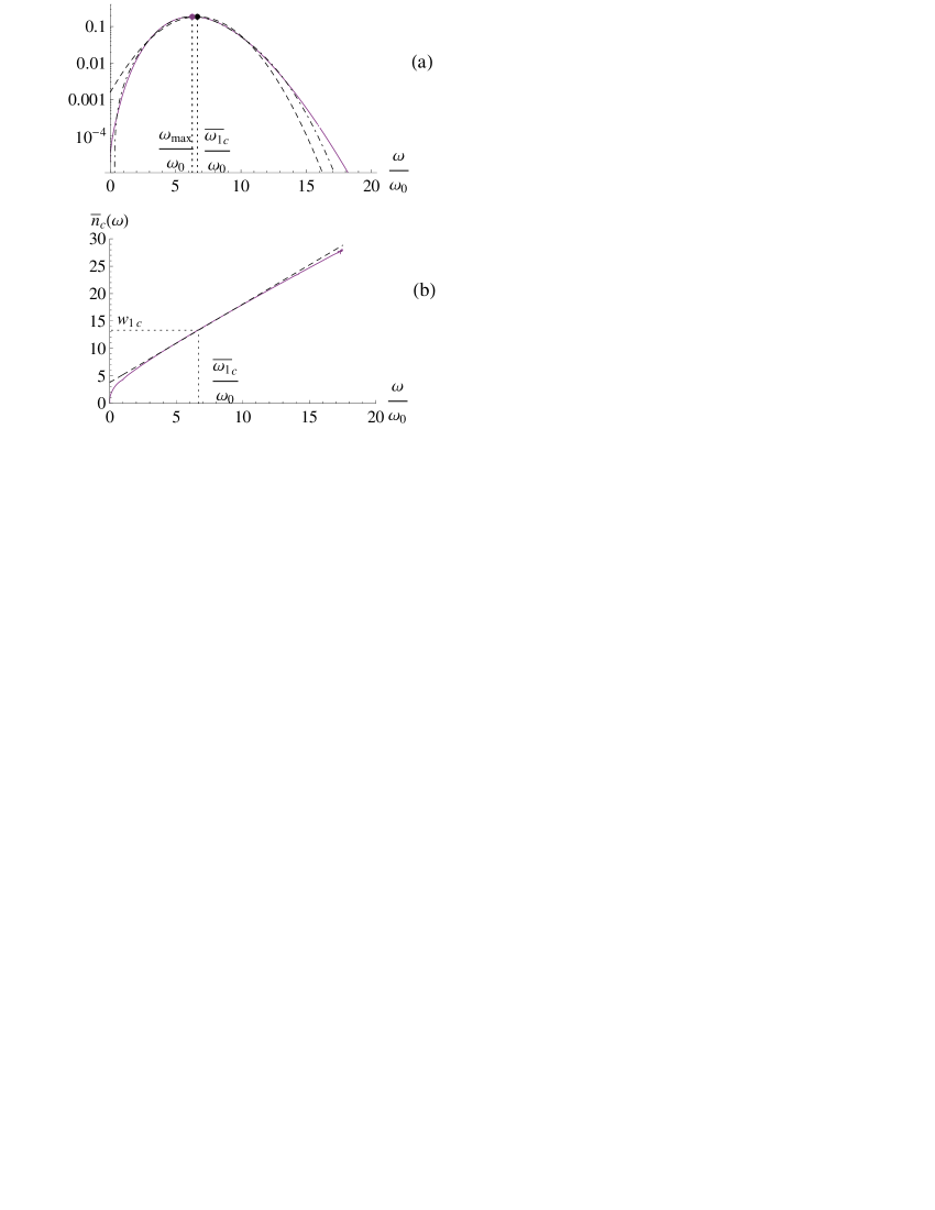
Figure 10: (a) Log plot of the resummed pure coherent radiation spectrum, at intensity parameter $b\omega_{0}=20$. Solid purple curve, exact distribution evaluated by Eqs. (103), (57–58). Dashed black curve, Gaussian approximation (113). Dot-dashed black curve, Gaussian approximation with Chebyshev correction (120). (b) Photon multiplicity spectrum under same conditions. Dashed black line, approximation (117).

The encountered integral still depends on rather many parameters, but under the high-intensity condition $\overline{\omega_{1}\!}_{\text{c}}\gg\sqrt{\overline{\omega^{2}_{1}}_{\text{c}}}$, their number can be effectively reduced. The upper limit of the integral is always on the right of the maximum of the Gaussian entering the integrand, hence at the upper integration limit, the Gaussian is decreasing. Granted that this decrease is rapid, one can replace this integration limit by infinity, unless the integration interval is too short. More precisely, the Gaussian varies across the integration interval significantly if

$$e^{-\frac{\left(\omega-\overline{\omega_{1\!}}_{\text{c}}\right)^{2}}{2\overline{\omega^{2}_{1\!}}_{\text{c}}}}\gg e^{-\frac{\overline{\omega_{1\!}}_{\text{c}}^{2}}{2\overline{\omega^{2}_{1\!}}_{\text{c}}}},$$ (125)

i.e.,

$$\omega\gg\frac{\overline{\omega^{2}_{1\!}}_{\text{c}}}{\overline{\omega_{1\!}}_{\text{c}}}.$$ (126)

Condition (126) is not very restrictive as long as its r.h.s. is independent of the radiation intensity, while its l.h.s. is typically $\sim\overline{\omega_{1\!}}_{\text{c}}\propto b$.

Thus, in the high photon multiplicity limit, it appears legitimate virtually at all $\omega$ to replace the upper integration limit in Eq. (124) by infinity. Therewith, utilizing the value of the integral

$$\int_{0}^{\infty}\frac{ds}{s^{1-a}}e^{-(s-\rho)^{2}/2}=\Gamma(a)e^{-{\rho^{2}}/4}D_{-a}(-\rho)$$ (127)

defining parabolic cylinder function $D_{-a}$ Abr-Stig ; Olver , we arrive at the closed-form representation

$$\frac{dw}{d\omega}\approx\frac{\Gamma(1+a)\Phi(a)}{\sqrt{2\pi}E^{a}\overline{\omega^{2}_{1\!}}_{\text{c}}^{\frac{1-a}{2}}}e^{-\rho^{2}/4}D_{-a}\left(-\rho\right).$$ (128)

Since function (128), similarly to (113), depends on $\omega$ only through a linearly related variable $\rho$, this may be regarded as extension of the scaling property beyond the vicinity of the maximum. But it should be remembered that the spectrum shape also depends on parameter $a$, so here we have a 2-parameter scaling. The corresponding functions, though, differ from Lévy distributions, rather being intermediate between Lévy distributions and Gaussian distributions.

The accuracy of approximation (128) may be assessed from Fig. 11a. There one observes that the parabolic cylinder approximation (dashed black curve) holds fairly well almost everywhere, except the small-$\omega$ limit.

Based on the obtained compact formula (128), we may now assess the deviation from the Gaussian behavior in the central region. In our equations, parameter $a$ must always remain small, and it is straightforward to check from definition (127) that $\underset{a\to+0}{\lim}D_{-a}(-\rho)=e^{-\rho^{2}/4}$, wherefore, at $a\to 0$ distribution (128) returns to Gaussian form (113). In the next approximation, the maximum of function (127) satisfies the equation

$$\frac{\partial}{\partial\rho}\int_{0}^{\infty}\frac{ds}{s^{1-a}}e^{-(s-\rho)^{2}/2}\qquad\qquad\qquad\qquad\qquad\qquad\,\,$$

$$=\int_{0}^{\infty}\!dss^{a}e^{-(s-\rho)^{2}/2}-\rho\int_{0}^{\infty}\!\frac{ds}{s^{1-a}}e^{-(s-\rho)^{2}/2}=0.\quad$$ (129)

At small $a$, the solution of Eq. (IV.3) is small, too, and in the linear approximation it equals

$$\rho_{\max}=\frac{\int_{0}^{\infty}dse^{-s^{2}/2}}{\int_{0}^{\infty}dss^{a-1}e^{-s^{2}/2}}+\mathcal{O}(a^{2})=a\sqrt{\frac{\pi}{2}}+\mathcal{O}(a^{2}).$$ (130)

In terms of $\omega$, it casts as

$$\omega_{\max}\simeq\overline{\omega_{1\!}}_{\text{c}}+a\sqrt{\frac{\pi}{2}\overline{\omega^{2}_{1\!}}_{\text{c}}}.$$ (131)

One may as well add here the skewness correction (122) (provided both corrections are small), getting:

$$\omega_{\max}\simeq\overline{\omega_{1\!}}_{\text{c}}-\frac{\overline{\omega^{3}_{1\!}}_{\text{c}}}{2\overline{\omega^{2}_{1\!}}_{\text{c}}}+a\sqrt{\frac{\pi}{2}\overline{\omega^{2}_{1\!}}_{\text{c}}}.$$ (132)

Note that those corrections have opposite signs, i.e., the incoherent radiation component gives a blueshift, while skewness a redshift, and they partially compensate each other. Evaluating the second derivative in the maximum, one can also show that the effect of $a$ is to broaden the spectrum.

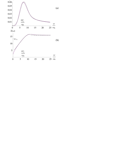
Figure 11: (a) Resummed radiation spectrum for coherent component described by Eqs. (57–58) with $b\omega_{0}=20$, and incoherent radiation component with $a=0.3$, $E=100\,\omega_{0}$. Solid purple curve, exact distribution; dashed black curve, parabolic cylinder approximation (128). (b) The photon multiplicity spectrum for same conditions as (a), and $\epsilon=0.1\omega_{0}$. Dashed black curve, parabolic cylinder approximation (135). Dot-dashed black curve, high-$\omega$ asymptotics (91).

At large $\omega$, the spectrum deviates from a Gaussian strongly, developing a power-law ‘tail’. The parabolic cylinder function at large values of its argument has asymptotics

$$e^{-\rho^{2}\!/4}D_{-a}(-\rho)\!\underset{\rho\to+\infty}{=}\!\frac{\sqrt{2\pi}}{\Gamma(a)\rho^{1-a}}\!\left[1\!+\!\mathcal{O}\!\left(\rho^{-2}\right)\!\right]+\mathcal{O}\!\left(\!e^{-\rho^{2}\!/2}\right)\!,$$

entailing for the spectrum

$$\frac{dw}{d\omega}\underset{\omega\to+\infty}{\simeq}\frac{a\Phi(a)}{E^{a}(\omega-\overline{\omega_{1\!}}_{\text{c}})^{1-a}}.$$ (133)

That agrees with Eq. (88) modulo exponentially small terms.

The calculation of $\bar{n}(\omega)$ proceeds along the same lines when based on convolution relation (III.3.1). Employing there Gaussian approximations (113), (117) along with power-law and logarithmic expressions (45), (55) for the pure incoherent component, we are led to the integral representation

$$\bar{n}(\omega)\approx\frac{1}{dw/d\omega}\frac{a\Phi(a)}{\sqrt{2\pi\overline{\omega^{2}_{1\!}}_{\text{c}}}}\qquad\qquad\qquad\qquad\qquad\quad$$

$$\times\!\int_{0}^{\omega}\frac{d\omega^{\prime}}{\omega^{\prime}}\left(\frac{\omega^{\prime}}{E}\right)^{a}e^{-\frac{\left(\omega-\overline{\omega_{1\!}}_{\text{c}}-\omega^{\prime}\right)^{2}}{2\overline{\omega^{2}_{1\!}}_{\text{c}}}}\Bigg{[}\nu(a)+a\ln\frac{\omega^{\prime}}{\epsilon}\qquad$$

$$+w_{1\text{c}}+\frac{\overline{\omega_{1\!}}_{\text{c}}}{\overline{\omega^{2}_{1\!}}_{\text{c}}}\left(\omega-\overline{\omega_{1\!}}_{\text{c}}-\omega^{\prime}\right)\Bigg{]}.\quad$$ (134)

By the same reasoning as for Eq. (124), the upper integration limit here may be extended to infinity. Evaluation of the integral gives the result

$$\bar{n}(\omega)\approx w_{1\text{c}}+\frac{\overline{\omega_{1\!}}_{\text{c}}}{\sqrt{\overline{\omega^{2}_{1\!}}_{\text{c}}}}R_{a}(\rho)+S_{a}(\rho)+a\ln\frac{\sqrt{\overline{\omega^{2}_{1\!}}_{\text{c}}}}{\epsilon},$$ (135)

where

$$R_{a}(\rho)=\rho-a\frac{D_{-1-a}(-\rho)}{D_{-a}(-\rho)},$$ (136)

and

$$S_{a}(\rho)=a\frac{\partial}{\partial a}\ln D_{-a}(-\rho)-a\gamma_{\text{E}}.$$ (137)

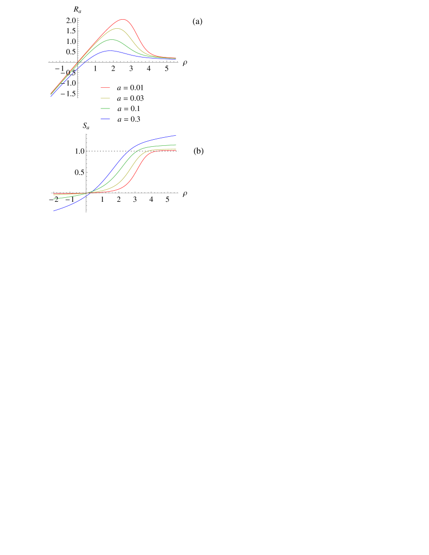
Figure 12: (a) Plots of function $R_{a}(\rho)$, for parameter $a=0.01$, 0.03, 0.1, 0.3 (top to bottom). (b) Plots of $S_{a}(\rho)$ for same values of $a$.

Shapes of functions (136), (137) for several values of parameter $a$ are illustrated in Figs. 12a,b. Function $S_{a}(\rho)$ appears to be monotonous, though step-like, whereas $R_{a}(\rho)$ features a hump. The maximum of $R_{a}(\rho)$ rises with the decrease of parameter $a$, though only logarithmically. Note that function $R_{a}$ enters Eq. (135) with a large coefficient, thence the shape of the maximum of $\bar{n}(\omega)$ is primarily described by $R_{a}(\rho)$. An additive correction comes from $S_{a}(\rho)$, whose unit jump in the turnover region of $R_{a}(\rho)$ partially compensates the drop of the photon multiplicity spectrum beyond its maximum.

The analysis of behavior of functions (136), (137) is alleviated by the knowledge of their values in the origin,

$$R_{a}(0)=-\frac{a}{\sqrt{2}}\frac{\Gamma\left(\frac{1+a}{2}\right)}{\Gamma\left(1+\frac{a}{2}\right)}$$ (138)

$$S_{a}(0)=-a\left[\frac{1}{2}\psi\left(\frac{1+a}{2}\right)+\frac{1}{2}\ln 2+\gamma_{\text{E}}\right],$$ (139)

and asymptotics at large $|\rho|$:

$$R_{a}(\rho)=\rho-\mathcal{O}(a/\rho)\qquad(\rho\to-\infty),$$ (140)

$$R_{a}(\rho)=\frac{2(1-a)}{\rho}+\mathcal{O}\left(\rho^{-3},\frac{\rho}{a}e^{-\rho^{2}/2}\right)\qquad(\rho\to+\infty),$$ (141)

$$S_{a}(\rho)\simeq-a\ln|\rho|\qquad(\rho\to-\infty),$$ (142)

$$S_{a}(\rho)\simeq a\ln\rho+\nu(a)\qquad(\rho\to+\infty),$$ (143)

with $\nu(a)$ defined by Eq. (56a). At $\rho\to+\infty$, i.e. asymptotic trans-central $\omega$, function $S_{a}(\rho)$ dominates, and along with terms $w_{1\text{c}}+a\ln\frac{\sqrt{\overline{\omega^{2}_{1\!}}_{\text{c}}}}{\epsilon}$ reproduces result (91).

Finally, we recall that the humpy structure of $\bar{n}(\omega)$ manifested itself already at moderate radiation intensity (cf. Fig. 8c). That may be non-accidental, since according to Ineq. (109), the accuracy of the saddle-point approximation improves at large $\omega$, where the maximum of $\bar{n}(\omega)$ is achieved.

V Reconstruction of single-photon spectrum from the multiphoton one

Although measurements of radiation spectra by the calorimetric method are ubiquitous, for further applications of the extracted photon beam it is often preferable to describe it in terms of photon number spectrum (II.1), anyway. Needless to say, the rate of any reaction (such as $e^{+}e^{-}$ creation or nuclear reactions) caused by a photon beam in a target is proportional to the photon number per energy interval, irrespective of temporal correlations between photons. Besides that, if the radiation spectrum is used for diagnostics of the radiator, the single-photon spectrum is more directly related to the classical radiation spectrum and the charged particle trajectory, and hence to the radiator parameters, than the multiphoton one.

Thus, there arises a need for reconstructing single-photon spectra from calorimetrically measured spectra. Such a problem had been addressed some time ago in Kolchuzhkin , where a procedure for reconstructing first moments (the mean and the variance) of the single-photon spectra from those of a multiphoton spectra was proposed. Here we will develop a reconstruction procedure for the complete spectrum. The prerequisite, however, is fair independence of the spectrum on initial state parameters to be averaged over, wherewith the outcoming multiphoton spectrum is representable purely by contour integral (17). As was argued in Sec. III.2, such conditions can be met for coherent bremsstrahlung or undulator radiation, but are unlikely for channeling radiation.

Let us begin with the observation that integral relation (15), with the aid of Eq. (10) can be cast in form where the l.h.s. depends only on $\frac{dw_{1}}{d\omega_{1}}$, while the r.h.s. only on $\frac{dw}{d\omega}$:

$$e^{\int_{0}^{E}d\omega_{1}\frac{dw_{1}}{d\omega_{1}}\left(e^{-s\omega_{1}}-1\right)}=1+\int_{0}^{E_{e}}d\omega\frac{dw}{d\omega}\left(e^{-s\omega}-1\right).$$ (144)

(As long as $\frac{dw}{d\omega}$ is supposed to be inferred from experimental data, the upper limit of integration over $\omega$ is set to $E_{e}$, which is the physical end of the spectrum.) To further obtain a linear integral equation for the single-photon spectrum, it suffices to take the logarithm of both sides of Eq. (144):

$$\int_{0}^{E}d\omega_{1}\frac{dw_{1}}{d\omega_{1}}\left(e^{-s\omega_{1}}-1\right)\qquad\qquad\qquad\qquad$$

$$=\ln\left[1+\int_{0}^{E_{e}}d\omega\frac{dw}{d\omega}\left(e^{-s\omega}-1\right)\right].$$ (145a)

After integration in the l.h.s. by parts, this can also be written

$$-s\int_{0}^{E}d\omega_{1}e^{-s\omega_{1}}\int^{E}_{\omega_{1}}d\omega^{\prime}_{1}\frac{dw_{1}}{d\omega^{\prime}_{1}}\qquad\qquad\qquad\quad$$

$$=\ln\left[1+\int_{0}^{E_{e}}d\omega\frac{dw}{d\omega}\left(e^{-s\omega}-1\right)\right].\,\,$$ (145b)

If $w_{1}$ is IR-finite, one can deal with Eq. (145) arranged with the aid of relation (10) in a simple form

$$\int_{0}^{E}d\omega_{1}\frac{dw_{1}}{d\omega_{1}}e^{-s\omega_{1}}=\ln\frac{1+\int_{0}^{E_{e}}d\omega\frac{dw}{d\omega}\left(e^{-s\omega}-1\right)}{1-\int_{0}^{E_{e}}d\omega\frac{dw}{d\omega}}.$$ (146)

Since here the l.h.s. is merely a Laplace transform of $\frac{dw_{1}}{d\omega_{1}}$, it inverts in the standard way:

$$\frac{dw_{1}}{d\omega_{1}}\! = \!\frac{1}{2\pi i}\int^{c+i\infty}_{c-i\infty}\!dse^{s\omega_{1}}\!\ln\!\left(\!1\!+\!\frac{\int_{0}^{E_{e}}d\omega\frac{dw}{d\omega}e^{-s\omega}}{1-\int_{0}^{E_{e}}d\omega\frac{dw}{d\omega}}\!\right)\,\,\,$$ (147b)

$$\equiv \!\frac{1}{2\pi i}\int^{c+i\infty}_{c-i\infty}\!dse^{s\omega_{1}}\!\ln\!\left(\int_{0}^{E_{e}}d\omega\frac{dw}{d\omega}e^{-s\omega}+W_{0}\!\right)\,\,$$

$$-\ln W_{0}\delta(\omega_{1})$$

$$(\omega_{1}<E).$$

Now, for $$\omega_{1}>0 \delta w_{1} w_{1} W_{0} W_{0}=1-\int_{0}^{E_{e}}d\omega\frac{dw}{d\omega}\to 0 \delta$$ (when the -term does not contribute), IR divergences do not appear in Eq. (147b), so the initial assumption of IR finiteness of may be relaxed. Eqs. (147) might as well be derived from Eq. (145), which is a bit more lengthy (solving a 1st-order differential equation), but does not need presuming IR finiteness of . If is finite, integral (147b) converges better, since the logarithm in the integrand vanishes at infinite integration limits. On the contrary, if , representation (147b) is untenable, and (147b) (without the -term) is the representation of choice.

From our experience with the resummation procedure in Sec. II, one may expect ambiguity in the contour integral representation for the reconstructed spectrum, as well. Indeed, applying Lemma 1 with $\mathcal{F}(z)=\ln(1+z/W_{0})$, or $\mathcal{F}(z)=\ln(W_{0}+z)$, one can see that the upper integration limit for the Laplace transform of $\frac{dw}{d\omega}$ in (147) may be an arbitrary number greater than $\omega_{1}$, e.g. equal $\omega_{1}+0$:

$$\frac{dw_{1}}{d\omega_{1}} = \frac{1}{2\pi i}\int^{c+i\infty}_{c-i\infty}dse^{s\omega_{1}}\ln\!\left(\int_{0}^{\omega_{1}+0}\!d\omega\frac{dw}{d\omega}e^{-s\omega}+W_{0}\right)$$ (147c)

$$-\ln W_{0}\delta(\omega_{1}).$$

Relation $\omega_{1}>\omega$ in integral (147c) may seem to be physically counterintuitive, because it is energetically anti-ordered. But as we emphasized in Sec. II.2, the energetic ordering property does not hold exactly for our distributions, anyway.

Another way to arrive at Eq. (147c) is to expand the logarithm in Eq. (147b) to power series, and evaluate the contour integral termwise:

$$\frac{dw_{1}}{d\omega_{1}}=\sum^{\infty}_{n=1}\frac{(-1)^{n-1}}{n\left(1-\int_{0}^{E_{e}}d\omega\frac{dw}{d\omega}\right)^{n}}\int_{0}^{E_{e}}d\Omega_{1}\frac{dw}{d\Omega_{1}}\ldots$$

$$\times\int_{0}^{E_{e}}d\Omega_{n}\frac{dw}{d\Omega_{n}}\delta\left(\omega_{1}-\sum_{k=1}^{n}\Omega_{k}\right).\qquad$$ (148a)

Here, as in passing from Eq. (9) to (II.1), one may replace upper limits $$E_{e} \omega_{+}0$$ by :

$$\frac{dw_{1}}{d\omega_{1}}=\sum^{\infty}_{n=1}\frac{(-1)^{n-1}}{n\left(1-\int_{0}^{E_{e}}d\omega\frac{dw}{d\omega}\right)^{n}}\int_{0}^{\omega_{1}+0}d\Omega_{1}\frac{dw}{d\Omega_{1}}\ldots$$

$$\times\int_{0}^{\omega_{1}+0}d\Omega_{n}\frac{dw}{d\Omega_{n}}\delta\left(\omega_{1}-\sum_{k=1}^{n}\Omega_{k}\right).\qquad$$ (148b)

In contrast to Eq. (9), however, series (148) involves no factorial in the denominator, whence it must have a finite convergence radius, such that $w_{1}\lesssim 1$. The latter property is natural, as long as resummed spectra are always bounded from above (see Sec. III.2.1, III.3.2). Series (148) at sufficiently small intensities of $w_{1}$ may prove to be actually even more convenient than contour integral representations (147). In particular, in the limit $\omega_{1}\to 0$, only the first term of (148) survives, giving

$$\frac{dw_{1}}{d\omega_{1}}\bigg{|}_{\omega_{1}=0}=\frac{\frac{dw}{d\omega}\big{|}_{\omega=0}}{1-\int_{0}^{E_{e}}d\omega\frac{dw}{d\omega}},$$ (149)

which is equivalent to Eq. (64). Keeping $\mathcal{O}(\omega_{1})$ terms, one can derive an analog of Eq. (65), etc.

For application of contour integral representations (147), it is also highly desirable to map singularities, as well as sectors of growth and decrease of the integrand, to which the integration contour can be adjusted. As long as the radiation spectrum obeys Eq. (146), the integrand singularities in Eqs. (147) must coincide with those of Laplace transform of the single-photon spectrum. But the latter transform may not have singularities in the right half-plane, since $\int^{\infty}d\omega_{1}\frac{dw_{1}}{d\omega_{1}}e^{-s\omega_{1}}$ converges at any positive $\mathfrak{Re}s$, so it is an analytic function of $s$ at $\mathfrak{Re}s>0$. In case if with the increase of $\omega_{1}$, $\frac{dw_{1}}{d\omega_{1}}$ decreases faster than exponentially [e.g., strictly vanishes beyond a coherent emission edge $\omega_{0}$, like in Eq. (57)], the l.h.s. of (146) exists at any $s$, so no singularities in the $s$ plane can emerge at all. In case if $\frac{dw_{1}}{d\omega_{1}}$ decreases with $\omega_{1}$ exponentially, its Laplace transform possesses singularities at finite negative $\mathfrak{Re}s$. Finally, if $\frac{dw_{1}}{d\omega_{1}}$ decreases by a power law, the l.h.s. of (146) diverges at $s<0$, so a singularity is situated at point $s=0$.

As concerns the convergence sectors, the integrand of (147b) obviously diverges at $\mathfrak{Re}s\to+\infty$ because of factor $e^{s\omega_{1}}$. At $\mathfrak{Re}s\to-\infty$, the integrand may decrease only provided the argument of the logarithm, after analytic continuation to the negative $\mathfrak{Re}s$ half-plane, does not increase faster than exponentially. In the latter case, the integration contour may be deformed to shape $\mathcal{C}_{2}$ (see Fig. 4). But that appears to be impossible in the important case when $\frac{dw_{1}}{d\omega_{1}}$ is anticipated to decrease at $\omega_{1}\to\infty$ faster than exponentially (e.g., pure single-harmonic coherent radiation). Then, as we noted above, the integrand of (147) may not have singularities in the whole complex plane, so if the integration contour might be deformed to $\mathcal{C}_{2}$, the result of the integration would identically equal zero, which is a clear contradiction. In this case, the only option for the integration contour in Eqs. (147) is a line parallel to the imaginary axis ($\mathcal{C}_{1}$).

At practice, when $\frac{dw}{d\omega}$ is measured as a number of events per bin of deposited energy, in Eq. (147b) the integral involving $\frac{dw}{d\omega}$ must be replaced by the corresponding finite sum. That is harmless for evaluation of the contour integrals, since the resulting function of $s$ remains analytic in the $s$ plane. But it is mandatory that the spectrum measurements are absolute, providing correct normalization of the spectrum.

At high intensity, when any resummed coherent spectrum tends to Gaussian form, our reconstruction method will ultimately become unsustainable. To appreciate the encountered difficulties, consider a toy model for the single-photon spectrum:

$$\frac{dw_{1}}{d\omega_{1}}=be^{-\Lambda\omega_{1}}$$ (150)

(with $E_{e}\to\infty$). The corresponding resummed spectrum evaluates in terms of a modified Bessel function:

$$\frac{dw}{d\omega}=\sqrt{\frac{b}{\omega}}e^{-\Lambda\omega-\frac{b}{\Lambda}}I_{1}(2\sqrt{b\omega}).$$ (151)

Laplace transform thereof equals

$$\int_{0}^{\infty}d\omega\frac{dw}{d\omega}e^{-s\omega}=e^{-\frac{b}{\Lambda}}\left(-1+e^{\frac{b}{\Lambda+s}}\right).$$

Now suppose that a calorimetric spectrum measurement gave instead of $\frac{dw}{d\omega}$ some slightly deviating distribution $\frac{dw}{d\omega}+\delta\frac{dw}{d\omega}$. Inserting this to Eq. (147b) leads to the reconstructed underlying spectrum

$$\frac{dw_{1}}{d\omega_{1}}\!=\!\frac{1}{2\pi i}\!\int^{c+i\infty}_{c-i\infty}\!dse^{s\omega_{1}}\!\ln\!\frac{e^{-\frac{bs}{\Lambda(\Lambda+s)}}\!+\!\int_{0}^{\infty}\!d\omega\!\left(e^{-s\omega}\!-\!1\right)\!\delta\frac{dw}{d\omega}}{e^{-\frac{b}{\Lambda}}-\int_{0}^{\infty}d\omega\delta\frac{dw}{d\omega}}.$$

Clearly, as $b$ increases, signal term $e^{-\frac{bs}{\Lambda(\Lambda+s)}}$ becomes exponentially small, and ultimately inferior to the error term; hence, for sufficiently large $b/\Lambda$ the method will loose efficiency. The best one can do in this situation, probably, is to extract first spectral moments as in Ref. Kolchuzhkin , which may appear insufficient for complete characterization of a highly structured single-photon spectrum.

In the latter straitened circumstances, it may also be worth engaging information contained in the photon multiplicity spectrum $\bar{n}(\omega)$. Examination of structure of integral (39) shows that it is more complicated than (17), and does not allow expressing $dw_{1}/d\omega_{1}$ explicitly. But in the high-multiplicity limit, when the reconstruction method based on $dw/d\omega$ is obstructed, one can at least extract from $\bar{n}(\omega)$ an additional parameter $w_{1\text{c}}$, say, through Eq. (118). Its knowledge, along with the knowledge of moments $\overline{\omega_{1\!}}_{\text{c}}$ and $\overline{\omega^{2}_{1\!}}_{\text{c}}$ (and possibly $\overline{\omega^{3}_{1\!}}_{\text{c}}$) extracted from $\frac{dw}{d\omega}$, may constrain the shape of $dw_{1}/d\omega_{1}$ more tightly.

VI Summary and outlook

The techniques developed in the present paper can be further employed to calculate spectra of specific coherent radiation sources, including channeling radiation. For undulator radiation, and partially for coherent bremsstrahlung, the results presented in this paper may already be applicable directly. Let us summarize the main physical lessons learned at this stage:

• The fundamental maximum of the multiphoton spectrum does not rise indefinitely with the increase of the radiator length $L$, but eventually saturates, and subsequently decreases. Instead, there is an elevation of the spectrum beyond the fundamental maximum, and its general spread (Sec. III). The high-$\omega$ spectral tail due to incoherent bremsstrahlung is the least affected by multiphoton effects, and its ratio w.r.t. the fundamental maximum thereby increases.

• Multiphoton effects alone can give rise to a second maximum in the coherent radiation spectrum, at $\omega\approx 2\omega_{0}$, even when secondary harmonics in the single-photon spectrum are absent.

• The low-$\omega$ part of the multiphoton spectrum, as well as discontinuities of the spectrum for coherent radiation, are suppressed by the factor of photon non-emission probability (Sec. III). Therein, manifestations of the incoherent radiation component in the spectrum are particularly pronounced.

• At high radiation intensity (in a long radiator), the resummed spectrum of pure coheernt radiation tends to a Gaussian form. But under presence of an incoherent component, it features a power-law tail towards large $\omega$ (Sec. IV). Such a diffusion regime may be regarded as weakly anomalous (characterized by $0<a\ll 1$). The corresponding limiting multiphoton spectrum is described by a parabolic cylinder function, being an intermediate asymptotic case between Gaussian and Lévy distributions.

• The photon multiplicity spectrum $\bar{n}(\omega)$ is an informative observable complementary to $\frac{dw}{d\omega}$, and is measurable with the modern state of the technology. The growth of $\bar{n}(\omega)$ with $\omega$ at low radiation intensity is stepwise, whereas at high intensity it smoothens out and tends to a linear law. In the region where the incoherent contribution overtakes the coherent one, $\bar{n}(\omega)$ saturates, and slightly subsides, whereupon continues rising, but only logarithmically (Secs. III, IV).

Promising are also the formulas for reconstruction of the single-photon spectrum from the calorimetrically measured one, derived in Sec. V. The applications thereof will be considered elsewhere.

It should also be remembered that although the present framework is well suited for fast evaluation of multiphoton emission effects, it is limited to conditions of soft radiation, which do not yet cover all the variety of interesting physical problems (e.g., hard coherent electromagnetic cascades, with deposited energies close to $E_{e}$, investigated in experiments Belkacem ). Nonetheless, for practical coherent radiation sources, as discussed in Appendix B and the beginning of Sec. IV, conditions of soft radiation are quite typical. At the same time, albeit many experiments in the soft radiation domain found multiphoton effects to be appreciable, none of those experiments addressed multiphoton effects systematically. The need for such dedicated experimental studies thus remains acute.

Appendix A Evaluation of the effective UV cutoff parameter

In Sec. III.1, we introduced parameter $E=\kappa E_{e}$ as an effective UV cutoff for the single-photon scale-invariant incoherent bremsstrahlung spectrum. The value of this parameter can be inferred from a theory accurately describing acts of large radiative energy loss. For our purposes, we need only the NLL soft asymptotics of this theory. As long as we deal solely with spectrum $\frac{dw}{d\omega}$ (and are not concerned with the photon multiplicity spectrum), the coherent radiation component at large $\omega$ can be entirely neglected. Thereby, we return to the well-known electromagnetic cascade theory in an amorphous medium, but with the due account of the electron spin.

For the single-photon bremsstrahlung spectrum, instead of (44) we take the ultra-relativistic and completely screened approximation of the Bethe-Heitler formula:

$$\frac{dw_{1\text{i}}}{d\omega_{1}}=\frac{a}{\omega_{1}}W_{\text{BH}}\left(\frac{\omega_{1}}{E_{e}}\right),$$ (152)

where Rossi

$$W_{\text{BH}}(z)=1-z+\frac{3}{4}z^{2}.$$ (153)

For simplicity, the pair production process will be neglected, as before. Then, the kinetic equation for electron energy distribution $\Pi(\mathcal{E})$ remains one-component:

$$\frac{\partial\Pi(\mathcal{E},a)}{\partial a}=\int_{\mathcal{E}}^{E_{e}}\frac{d\mathcal{E}^{\prime}}{\mathcal{E}^{\prime}-\mathcal{E}}\Pi(\mathcal{E}^{\prime},a)W_{\text{BH}}\left(\frac{\mathcal{E}^{\prime}-\mathcal{E}}{\mathcal{E}^{\prime}}\right)$$

$$-\Pi(\mathcal{E},a)\int_{0}^{\mathcal{E}}\frac{d\mathcal{E}^{\prime}}{\mathcal{E}-\mathcal{E}^{\prime}}W_{\text{BH}}\left(\frac{\mathcal{E}-\mathcal{E}^{\prime}}{\mathcal{E}}\right),$$ (154)

where dimensionless parameter $a$ is proportional to the target thickness [see Eq. (43)]. Integro-differential equation (A) is endowed with the initial condition (100):

$$\Pi(\mathcal{E},0)=\delta(\mathcal{E}-E_{e}).$$ (155)

Once the solution of Eq. (A–155) is attained, the multiphoton radiation spectrum, equal to the radiative energy loss spectrum, is determined by the correspondence rule (98):

$$\frac{dw_{\text{i}}}{d\omega}=\Pi(E_{e}-\omega,a)\qquad[W_{0}(a>0)=0],$$ (156)

and for this function we are interested in the limit $\omega\ll E_{e}$. Note that by a change of integration variables, Eq. (A) may can be recast

$$\frac{\partial}{\partial a}\Pi(E_{e}-\omega,a)=\int^{\omega}_{0}\frac{d\omega_{1}}{\omega_{1}}\Pi(E_{e}-\omega+\omega_{1},a)\qquad\qquad$$

$$\times W_{\text{BH}}\left(\frac{\omega_{1}}{E_{e}-\omega+\omega_{1}}\right)\qquad$$

$$-\Pi(E_{e}-\omega,a)\int_{0}^{E_{e}-\omega}\frac{d\omega_{1}}{\omega_{1}}W_{\text{BH}}\left(\frac{\omega_{1}}{E_{e}-\omega}\right),$$

which turns to recoilless kinetic equation (96) in the limit $\omega_{1}\ll E_{e}$, when $W_{\text{BH}}(z)\to W_{\text{BH}}(0)=1$. However, form (A) is more convenient for solution.

Solution of Eq. (A) is obtained by applying Mellin transform

$$\Pi(s,a)=\int_{0}^{E_{e}}d\mathcal{E}{\mathcal{E}}^{s-1}\Pi(\mathcal{E},a),$$ (157)

in terms of which the integro-differential equation becomes ordinary differential:

$$\frac{\partial}{\partial a}\Pi(s,a)=-\mu(s)\Pi(s,a),$$ (158)

with $a$-independent coefficient

$$\mu(s)=\int_{0}^{1}dz\frac{1-z^{s-1}}{1-z}W_{\text{BH}}(1-z)$$ (159)

and initial condition

$$\Pi(s,0)=E_{e}^{s-1}.$$ (160)

Integrating Eq. (158), and applying the inverse Mellin transform $\Pi(\mathcal{E},a)=\frac{1}{2\pi i}\int_{c-i\infty}^{c+\infty}ds{\mathcal{E}}^{-s}\Pi(s,a)$, leads to the solution

$$\Pi(\mathcal{E},a)=\frac{1}{E_{e}}\frac{1}{2\pi i}\int_{c-i\infty}^{c+\infty}dse^{-a\mu(s)+s\ln(E_{e}/\mathcal{E})}.$$ (161)

By correspondence rule (156), the multiphoton bremsstrahlung spectrum ensues

$$\frac{dw_{\text{i}}}{d\omega}=\frac{1}{E_{e}}\frac{1}{2\pi i}\int_{c-i\infty}^{c+\infty}dse^{-a\mu(s)+s\ln\frac{1}{1-\omega/E_{e}}}\qquad\quad$$

$$\simeq\frac{1}{\omega}\frac{1}{2\pi i}\int_{c-i\infty}^{c+\infty}d\zeta e^{\zeta-a\mu(\zeta E_{e}/\omega)}\qquad(\omega\ll E_{e}).\quad$$ (162)

In the last line, we linearized $\ln\frac{1}{1-\omega/E_{e}}\simeq\frac{\omega}{E_{e}}$ for small ${\omega}/{E_{e}}$ we are concerned with, and changed the integration variable to $\zeta=-s\omega/E_{e}$.

Function $\mu$ at large arguments needed for us increases logarithmically:

$$\mu(s)\equiv W_{\text{BH}}(0)\int_{0}^{1}dz\frac{1-z^{s-1}}{1-z}\qquad\qquad\qquad\qquad\qquad$$

$$+\int_{0}^{1}dz\frac{1-z^{s-1}}{1-z}[W_{\text{BH}}(1-z)-W_{\text{BH}}(0)]\qquad\qquad$$

$$=\ln s+\gamma_{\text{E}}+\!\int_{0}^{1}\!\frac{dz^{\prime}}{z^{\prime}}[W_{\text{BH}}(z^{\prime})\!-\!W_{\text{BH}}(0)]+\mathcal{O}\!\left(s^{-1}\right)\!.$$

Inserting this approximation to Eq. (A), and doing the elementary contour integral, from comparison with Eq. (45, 49) we ultimately infer the value for $\kappa$:

$$\kappa=e^{\int_{0}^{1}\frac{dz^{\prime}}{z^{\prime}}[W_{\text{BH}}(z^{\prime})-W_{\text{BH}}(0)]}=e^{-5/8}\approx 0.5.$$ (164)

According to Eq. (164), the effective UV cutoff must be set at about half the initial electron energy. With this value for $\kappa$, our Eqs. (45, 49) agree with Eqs. (2.11), (2.19) of BK .

Appendix B Estimates of photon multiplicities for coherent radiation sources

In this Appendix, we will collect equations for spectral parameters of main coherent radiation sources, needed for numerical estimates of significance of multiphoton effects in Sec. IV.

Any coherent radiation source we consider may be viewed as an ultrarelativistic electron (or positron) radiating under the influence of periodic force $F(t)$ (having period $T$), directed predominantly transverse to the electron’s large mean momentum (which is taken parallel to $Oz$). If the radiation is of dipole type, i.e. produced by a weakly accelerated electron remaining non-relativistic in its average rest frame (e.r.f.), the emitted electromagnetic radiation in this frame will be monochromatic. In e.r.f., period $T$ is Lorentz-contracted to $\widetilde{T}=T/\gamma$ ($\gamma$ stands for the electron Lorentz factor), corresponding to frequency $\widetilde{\omega}_{0}=\frac{2\pi}{\widetilde{T}}$. The radiation in the e.r.f. is not strictly isotropic, as long as the driving force is known to be transverse w.r.t. $Oz$. For our purposes, we need only the angular distribution averaged over the azimuthal angles, which will thus obey a $\propto 1+\cos^{2}\tilde{\theta}$ law, where $\tilde{\theta}$ is the angle between $Oz$ and the photon emission direction in e.r.f. This information suffices to write the angle-differential radiation intensity:

$$d\tilde{I}=e^{2}\left|\frac{1}{\widetilde{T}}\int^{\widetilde{T}/2}_{-\widetilde{T}/2}d\tilde{t}\frac{\widetilde{F}(\tilde{t})}{m}e^{-{2\pi i\tilde{t}}/{\widetilde{T}}}\right|^{2}\frac{1+\cos^{2}\tilde{\theta}}{2}\sin\tilde{\theta}d\tilde{\theta},$$ (165)

where $m$ and $e$ are the electron mass and charge. [To check the numerical coefficient, note that integration of (165) over photon emission angles with $\int_{0}^{\pi}\frac{1+\cos^{2}\tilde{\theta}}{2}\sin\tilde{\theta}d\tilde{\theta}=\frac{4}{3}$, and identification of $\frac{\widetilde{F}(\tilde{t})}{m}$ with the electron acceleration, leads to the famous Larmor formula.]

Eq. (165) gives an average (over the oscillation period) energy emitted by the electron in its rest frame per unit time. Dividing this by the photon energy $\widetilde{\omega}_{0}$ gives the probability density, and the total probability is obtained by multiplying by the period value and the number of periods $N$:

$$dw_{1\text{c}}=\frac{\widetilde{T}N}{\widetilde{\omega}_{0}}d\tilde{I}\equiv\frac{N}{2\pi}\widetilde{T}^{2}d\tilde{I}.$$

The latter quantity must be Lorentz invariant, which is opportune for expressing the desired radiation spectrum in the lab.

The advantage of referring to e.r.f. variables is that $\cos\tilde{\theta}$ is related to the photon momentum projection on the light front in $z$-direction, and therethrough to the photon energy in the lab frame:

$$\frac{\omega_{1}}{\omega_{0}}=\frac{1+\cos\tilde{\theta}}{2},$$ (166)

where $\omega_{0}$ is the maximal photon energy in the lab, corresponding to $\tilde{\theta}=0$. Expressing $\cos\tilde{\theta}$ from (166), inserting it to (165), and differentiating, we convert the angular distribution in e.r.f. to the spectral distribution in the lab:

$$dw_{1\text{c}}=\frac{e^{2}N}{\pi}\left|\int^{\widetilde{T}/2}_{-\widetilde{T}/2}d\tilde{t}\frac{\widetilde{F}(\tilde{t})}{m}e^{-{2\pi i\tilde{t}}/{\widetilde{T}}}\right|^{2}P\left(\frac{\omega_{1}}{\omega_{0}}\right)\frac{d\omega_{1}}{\omega_{0}},$$ (167)

with $P(z)$ being function (58), thus explaining its origin. Product $d\tilde{t}\widetilde{F}(\tilde{t})=dp_{\perp}$ entering the time integral is Lorentz invariant, too, so it can be written as $dtF(t)$, where $F$ is the force, and $t$ the time in the lab. Comparing (167) with Eq. (57), we infer

$$b\omega_{0}=\frac{e^{2}}{\pi}\left|\int^{T/2}_{-T/2}dt\frac{F(t)}{m}e^{-{2\pi it}/{T}}\right|^{2}N,$$ (168)

where $T$ is the motion period in the lab, and obviously, $N=L/T$.

Although product $b\omega_{0}$ is all we need for estimates of the photon multiplicity, it is also expedient to evaluate the photon energy scale $\omega_{0}$ independently. The latter is obtained from e.r.f. value $\widetilde{\omega}_{0}=\frac{2\pi\gamma}{T}$ by boosting along $Oz$ with the Lorentz factor $\gamma$. That results in multiplication by $\sqrt{\frac{1+v}{1-v}}\approx 2\gamma$, so the maximal photon energy in the lab equals

$$\omega_{0}\approx 2\gamma^{2}\frac{2\pi}{T},$$ (169)

exceeding by factor of $2\gamma^{2}$ the driving force frequency in this frame.

The analysis of photon multiplicity for specific radiation sources further reduces to estimating in Eq. (168) the driving force magnitude and period. Note that generally, the square of the integral in (168) is $\sim T^{2}$, while $N\sim T^{-1}$. Thus, in total, the radiation source brightness is proportional to its period. On the other hand, according to Eq. (169), the photon energy scales as $T^{-1}$, though that is generally compensable by an appropriate increase in $\gamma$.

B.1 Coherent bremsstrahlung

For an electron crossing a family of atomic planes by a near-straight trajectory at a small misalignment angle $\chi$, the time in Eq. (168) expresses as $t=x/\chi$, where $x$ is the coordinate transverse to the planes, and the oscillation period in the lab equals

$$T=\frac{d}{\chi},$$ (170)

$d$ being the plane spacing. Therewith, Eq. (168) becomes

$$b\omega_{0}=\frac{e^{2}}{\pi}\left|\int^{d/2}_{-d/2}\frac{dx}{\chi}\frac{F(x)}{m}e^{-{2\pi ix}/{d}}\right|^{2}\frac{L\chi}{d},$$ (171)

where $F$ as a function of time was replaced by the corresponding function of $x$. If $F(x)$ within a period describes roughly as

$$F(x)\approx\frac{2F_{\max}}{d}x\qquad(-d/2<x<d/2),$$ (172)

evaluation of the integral in Eq. (171) gives

$$b\omega_{0}=\frac{e^{2}F_{\max}^{2}d}{\pi^{3}m^{2}\chi}L\approx 6\cdot 10^{-5}\frac{L[\text{mm}]}{\chi},$$ (173)

where we used numerical estimates $d\approx 2\,\AA$, and $|F_{\max}|\approx 6\text{ GeV/cm}$.

Parameters $L$ and $\chi$ are not completely independent: they must obey inequality (cf. PDG )

$$\delta\chi=\frac{13.6\text{ MeV}}{E_{e}}\sqrt{\frac{L}{X_{0}}}\ll\chi,$$ (174)

in order for the multiple scattering spread $\delta\chi$ not to blur the coherent peak. At the same time, $\chi$ correlates with $E_{e}$, since under assumption $\omega_{0}\ll E_{e}$, Eqs. (169, 170) yield

$$E_{e}\chi\ll\frac{m^{2}d}{4\pi}=20\text{ MeV}.$$ (175)

For practical misalignment angles $10^{-2}<\chi<10^{-4}$, this constrains the electron energy to $1<E_{e}<100$ GeV. Eqs. (174) and (175) are only compatible provided $\sqrt{L/X_{0}}\ll 1$, which is essentially the condition (51) adopted in our paper.

B.2 Channeling radiation

For the case of channeling, the oscillation period depends on the particle energy:

$$T=2\pi\sqrt{\frac{E_{e}}{|\partial F/\partial x|}}.$$ (176)

For a harmonic potential [corresponding to force (172)], the period will be constant, but with the account of anharmonicity, it may acquire also some dependence on the particle transverse energy in the channel. For our estimates, it will suffice to adopt the harmonic approximation, letting

$$F(t)=F_{0}\cos\frac{2\pi t}{T},$$ (177)

where $F_{0}$ depends on the particle impact parameters, in the spirit of Eq. (172). As an order of magnitude estimate, we may use $F_{0}\sim F_{\max}/2$. Substituting (177) to Eq. (168), we get

$$b\omega_{0} = \frac{e^{2}}{4\pi m^{2}}F_{0}^{2}TL$$ (178a)

$$\sim \frac{e^{2}}{8m^{2}}\sqrt{\frac{E_{e}d}{2F_{\max}}}F_{\max}^{2}L.$$ (178b)

At practice, the length of a crystal for channeling is limited by dechanneling effects. For positrons, the dechanneling length may be estimated crudely as Ld-for-positrons

$$L_{\text{d}}\sim 0.5\frac{\text{mm}}{\text{GeV}}E_{e},$$ (179)

in terms of which Eq. (178b) assumes the form

$$b\omega_{0}\approx 8\left(E_{e}[\text{GeV}]\right)^{3/2}\frac{L}{L_{\text{d}}}.$$ (180)

B.3 Undulator radiation

In an undulator, the particle is moving in a fixed channel, similarly to channeling, but the motion period, determined by the magnet spacing, is energy-independent, like in coherent bremsstrahlung. Since $T$ is macroscopically large, according to Eqs. (168–169), the source must be bright, but the photon energy be relatively low. Nonetheless, gamma-range undulators were created recently, with periods $T\lesssim 1$ cm, and electron energies $\sim 10^{2}$ GeV Moortgat-Pick .

For description of the undulator field strength, it is customary to introduce parameter

$$K=\frac{eB_{0}}{m}\frac{T}{2\pi}\approx 1B_{0}[\text{T}]T[\text{cm}],$$ (181)

where $B_{0}$ is the field amplitude, $B(t)=B_{0}\sin\frac{2\pi t}{T}$. In terms of $K$, Eq. (168) reads

$$b\omega_{0}=\pi e^{2}K^{2}N\approx 0.02K^{2}N.$$ (182)

At practice, parameter $K$ can be $\sim 1$ (somewhat violating the dipole radiation condition $K\ll 1$), whilst the number of periods can amount several hundreds or thousands. The latter number is particularly large for undulator-based positron sources, where $N\sim 10^{4}$ Moortgat-Pick .

Appendix C High-intensity multiphoton spectrum in peripheral regions

As had been pointed out in Sec. IV.2.2, beyond the central region specified by condition (115), the Gaussian approximation breaks down, and the multiphoton spectrum becomes dependent on all the detail of the single-photon spectrum. Even though in those regions the radiation spectrum is relatively faint (and at high $\omega$ it may be overwhelmed by the incoherent bremsstrahlung ‘tail’), it may still prove measurable under high absolute radiation intensity. Therefore, it would be useful to find some approximations for peripheral regions, as well.

Suitable approximations for coherent radiation in peripheral regions can be built based on the same saddle-point approximation described in Sec. IV.2.1, provided transcendental saddle-point equation (IV.2.1) is solved at least approximately. That requires development of a special approach on each side from $\overline{\omega_{1\!}}_{\text{c}}$.

C.1 Trans-central region

Let us consider the region $\omega\gg\overline{\omega_{1\!}}_{\text{c}}$ first. From the viewpoint of Eq. (IV.2.1), this corresponds to large and negative $s_{0}$ (see Fig. 13). It is therefore beneficial to rewrite Eq. (IV.2.1) as

$$\ln\frac{\omega}{b\omega_{0}^{2}}+s_{0}\omega_{0}=\ln\left[\int_{0}^{1}dzzP(z)e^{-s_{0}\omega_{0}(z-1)}\right],$$ (183)

where the r.h.s. is smaller than any of the terms on the l.h.s. (granted that the exponential within the integration domain is $\leq 1$, achieving unity only at the endpoint $z=1$). Thence, the r.h.s. can be treated as a perturbation.

Figure 13: Graphical real solution of saddle-point equation (IV.2.1), for $\frac{dw_{1\text{c}}}{d\omega_{1}}$ given by Eqs. (57–58). Solid purple curve, exact solution. Dotted black line, central region approximation (112). Purple point, the central solution. Long-dashed black curve, large-$\omega$ approximation (185). Short-dashed black curve, improved large-$\omega$ approximation (C.1). Dot-dashed black curve, low-$\omega$ approximation (188).

To solve Eq. (183) iteratively, first, we express $s_{0}\omega_{0}$ from equating the l.h.s. to zero (leading log approximation):

$$-s_{0}\omega_{0}=\ln\frac{\omega}{b\omega_{0}^{2}}+\mathcal{O}\left(\ln\ln\frac{\omega}{b\omega_{0}^{2}}\right).$$ (184)

Substituting this to the r.h.s. of (183) gives a NLL approximation for $s_{0}\omega_{0}$:

$$s_{0}\omega_{0}=\ln\left[\int_{0}^{1}dzzP(z)\left(\frac{\omega}{b\omega_{0}^{2}}\right)^{z-2}\right]+\mathcal{O}\left(\ln\ln\ln\frac{\omega}{b\omega_{0}^{2}}\right).$$ (185)

Its behavior is illustrated in Fig. 13 by the long-dashed black curve. It does not seem to be accurate enough, which compels us to proceed to NNLL: substitute $s_{0}\omega_{0}$ in the r.h.s. of Eq. (183) by that expressed from the l.h.s., whereupon replace the remaining $s_{0}\omega_{0}$ in the r.h.s. by LL expression (184):

$$s_{0}\omega_{0}\simeq\ln\Bigg{\{}\int_{0}^{1}dzzP(z)\left(\frac{\omega}{b\omega_{0}^{2}}\right)^{z-2}\qquad\quad$$

$$\times\left[\int_{0}^{1}dyyP(y)\left(\frac{\omega}{b\omega_{0}^{2}}\right)^{y-1}\right]^{1-z}\Bigg{\}}.$$ (186)

The latter solution is to be inserted to Eqs. (106–107), which are then inserted to (108a). The resulting expression is rather bulky, and will be omitted. Its accuracy can be visualized from Fig. 13, and may be regarded as satisfactory. The qualitative corollary from Eq. (C.1) is that the multiphoton pure coherent spectrum decreases by the law close to linear exponential [since in (108a) $A\sim s_{0}\omega_{0}e^{-s_{0}\omega_{0}}$].

C.2 Sub-central region

The opposite peripheral region $\omega<\overline{\omega_{1\!}}_{\text{c}}$ corresponds to positive $s_{0}$ (see Fig. 13). There, the main contribution to the integral entering Eq. (IV.2.1) stems from the lower integration limit. Asymptotically, at large $s_{0}$,

$$\omega=\int_{0}^{\omega_{0}}d\omega_{1}\omega_{1}\frac{dw_{1\text{c}}}{d\omega_{1}}e^{-s_{0}\omega_{1}}=\frac{bP(0)}{s_{0}^{2}}+\mathcal{O}\left(\frac{bP(0)}{s_{0}^{3}\omega_{0}}\right),$$ (187)

but the latter asymptotic solution becomes accurate at $\omega\ll\overline{\omega_{1\!}}_{\text{c}}$ only, whereas we need to cover the whole region $\overline{\omega_{1\!}}_{\text{c}}-\omega\gg\overline{\omega^{2}_{1\!}}_{\text{c}}$. Therefore, Eq. (IV.2.1) needs to be solved accurately on the whole interval $0<\omega<\overline{\omega_{1\!}}_{\text{c}}$, which is challenging insofar as this equation is transcendental.

In the present situation, one of the simplest approaches may be to interpolate the solution between asymptotes (187) and (111), e.g., writing it in form

$$\omega\approx\frac{1}{\frac{1}{bP(0)}s_{0}^{2}+\frac{\overline{\omega^{2}_{1\!}}_{\text{c}}}{\overline{\omega_{1\!}}_{\text{c}}^{2}}s_{0}+\frac{1}{\overline{\omega_{1\!}}_{\text{c}}}}.$$ (188)

The behavior of the latter interpolation is illustrated in Fig. 13 by the dot-dashed black curve, which is rather close to the exact solution on the interval of interest. Expressing $s_{0}$ (or $s_{0}^{-1}$) from quadratic equation (188) and inserting to Eq. (106–107), we get an approximation holding up to the central region). Qualitatively, at large $s_{0}$, $A\sim\frac{2bP(0)}{s_{0}}-w_{1\text{c}}\sim 2\sqrt{b\omega}-w_{1\text{c}}$, which may be interpreted in the sense that the function rises faster than a Gaussian.

References

- (1) V.A. Bazylev and N.K. Zhevago, Usp. Fiz. Nauk 137 (1982) 605 [Sov. Phys. Usp. 25 (1982) 565]; H. Motz, P. Luchini. Undulators and free-electron lasers. Oxford: University Press, 1990; P. Rullhusen, X. Artru, P. Dhez. Novel Radiation Sources using Relativistic Electrons. World Scientific, 1998; A.P. Potylitsyn. Electromagnetic Radiation of Electrons in Periodic Structures. Springer, 2011.
- (2) B. Rossi and K. Greisen, Rev. Mod. Phys. 13 (1941) 240; W. Heitler. The Quantum Theory of Radiation, 3rd ed. Oxford: Clarendon Press, 1954.
- (3) See, e.g., V.N. Baier, V.M. Katkov, and V.M. Strakhovenko, NIM A 250 (1986) 514; NIM B 27 (1987) 360.
- (4) J.M. Jauch, F. Rohrlich. The theory of photons and electrons, 2nd ed. Springer, 1976; V.B. Berestetskii, E.M. Lifshitz, L.P. Pitaevskii, Quantum Electrodynamics. Oxford: Pergamon-Press, 1982; S. Weinberg. Quantum Field Theory, Vol. 1, 3rd ed., Cambridge: University Press, 1999.
- (5) G. Moortgat-Pick et al. Phys. Rep. 460 (2008) 131.
- (6) G. Knoll. Radiation detection and measurement, 4th ed. New York: Wiley, 2010; C. Grupen, B. Shwartz. Particle detectors, 2nd ed. Cambridge: University Press, 2008.
- (7) R. Wigmans. Calorimetry: Energy Measurement in Particle Physics. Oxford: Clarendon, 2000; R.M. Brown and D.J.A. Cockerill, NIM A 666 (2012) 47.
- (8) J. Beringer et al. (Particle Data Group), Phys. Rev. D 86 (2012) 010001.
- (9) G.L. Bochek et al. NIM B 173 (2001) 49.
- (10) L.D. Landau, J. Phys. USSR 8 (1944) 201.
- (11) F. Bloch and A. Nordsieck, Phys. Rev. 52 (1937) 54; D.R. Yennie, S.C. Frautschi, and H. Suura, Ann. Phys. (NY) 13 (1961) 379.
- (12) G. Parisi and R. Petronzio, Nucl. Phys. B 154 (1979) 427; J. Collins, D. Soper, and G. Sterman, Nucl. Phys. B 250 (1985) 199.
- (13) W. Feller. An Introduction to Probability Theory and Its Applications, Vol. II, New York: Wiley, 1971.
- (14) A.I. Akhiezer and N.F. Shul’ga, Zh. Eksp. Teor. Fiz. 85 (1983) 94 [Sov. Phys. JETP 58 (1983) 55].
- (15) V.N. Baier and V.M. Katkov, Phys. Rev. D 59 (1999) 056003.
- (16) M.Kh. Khokonov, Zh. Eksp. Teor. Fiz. 126 (2004) 799 [JETP 99 (2004) 690].
- (17) A.I. Akhiezer, V.I. Truten, and N.F. Shul’ga, Phys. Lett. A 123 (1987) 361.
- (18) V.N. Baier, V.M. Katkov, and V.M. Strakhovenko, Zh. Eksp. Teor. Fiz. 92 (1987) 1228 [Sov. Phys. JETP 65 (1987) 686]; NIM B 69 (1992) 258; NIM B 119 (1996) 131.
- (19) X. Artru, NIM B 48 (1990) 278.
- (20) Yu.V. Kononets and V.A. Ryabov, NIM B 48 (1990) 269, 274.
- (21) Yu.A. Chesnokov, V.I. Kotov, V.A. Maisheev, and I.A. Yazynin, JINST 3 (2008) P02005.
- (22) A. Apyan, NIM B 255 (2007) 269.
- (23) K. Kirsebom et al. NIM B 119 (1996) 79; A. Baurichter et al. Nucl. Phys. B (Proc. Suppl.) 44 (1995) 79; Phys. Rev. Lett. 79 (1997) 3415.
- (24) M.V. Bondarenco, Phys. Rev. A 82 (2010) 042273.
- (25) L. Mandel, E. Wolf. Optical coherence and quantum optics. Cambridge: University Press, 1995.
- (26) A.M. Kolchuzhkin, V.V. Uchaikin. Introduction to the Theory of Particle Passage through Matter (in Russian). Moscow: Atomizdat, 1978.
- (27) J. Bak et al. Nucl. Phys. B 254 (1985) 491.
- (28) R. Medenwaldt et al. Phys. Lett. B 260 (1991) 235.
- (29) A.G. Bonch-Osmolovsky and M.I. Podgoretsky, Yad. Fiz. 29 (1979) 432 [Sov. J. Nucl. Phys. 29 (1979) 216]; M.I. Podgoretsky, Yad. Fiz. 31 (1980) 417 [Sov. J. Nucl. Phys. 31 (1980) 218].
- (30) B.V. Gnedenko, A.N. Kolmogorov. Limit Distributions for Sums of Independent Random Variables. Cambridge, MA: Addison-Wesley, 1954.
- (31) M.V. Bondarenco, Phys. Rev. A 81 (2010) 052903; Nuov. Cim. C 34 (2011) 381; V.A. Maisheev, Nuov. Cim. C 34 (2011) 73; S. Bellucci and V.A. Maisheev, Phys. Rev. A 86 (2012) 042902; V. Guidi, L. Bandiera, and V. Tikhomirov, Phys. Rev. A 86 (2012) 042903.
- (32) A. Kolchuzhkin, A. Potylitsyn, A. Bogdanov, and I. Tropin, Phys. Lett. A 264 (1999) 202; A. Kolchuzhkin and A. Potylitsyn, NIM B 173 (2001) 126.
- (33) J.D. Jackson. Classical Electrodynamics, 3rd ed., New York: Wiley, 1998.
- (34) M.L. Ter-Mikayelyan. High Energy Electromagnetic Processes in Condensed Media. New York: Wiley, 1972.
- (35) G. Diambrini Palazzi, Rev. Mod. Phys. 40 (1968) 611.
- (36) N.G. Van Kampen. Stochastic Processes in Physics and Chemistry. North-Holland Personal Library, 2007.
- (37) V.G. Baryshevskii and I.Ya. Dubovskaya, Phys. Lett. A 62 (1977) 45; V. Tikhomirov, Phys. Lett. A 125 (1987) 411; X. Artru, Phys. Lett. A 128 (1988) 302; V.V. Beloshitsky, A.Kh. Khokonov, and M.A. Kumakhov, NIM B 62 (1991) 207.
- (38) A.I. Akhiezer and N.F. Shul’ga, Usp. Fiz. Nauk 137 (1982) 561 [Sov. Phys. Usp. 25 (1982) 541].
- (39) V.V. Beloshitsky and F.F. Komarov, Phys. Rep. 93 (1982) 117.
- (40) M.D. Bavizhev, Yu.V. Nil’sen, and B.A. Yur’ev, Zh. Eksp. Teor. Fiz. 95 (1989) 1392 [Sov. Phys. JETP 68 (1989) 803].
- (41) F.F. Ternovskii, Zh. Eksp. Teor. Fiz. 39 (1960) 171 [Sov. Phys. JETP 12 (1961) 123]; N.F. Shul’ga and S.P. Fomin, JETP Lett. 27 (1978) 117; H.D. Thomsen et al. Phys. Rev. D 81 (2010) 052003.
- (42) R. Medenwaldt et al. Phys. Lett. B 227 (1989) 483.
- (43) A. Apyan et al. Phys. Rev. ST-AB 11 (2008) 041001.
- (44) G. Alexander et al. NIM A 610 (2009) 451.
- (45) X. Artru et al. NIM B 240 (2005) 762.
- (46) J.-P. Bouchaud and A. Georges, Phys. Rep. 195 (1990) 127; R. Metzler and J. Klafter, Phys. Rep. 339 (2000) 1.
- (47) F.W.J. Olver. Asymptotics and Special Functions, 2nd ed. Taylor Francis, 1997.
- (48) M. Abramowitz, I.A. Stegun. Handbook of Mathematical Functions. New York: Dover (1972).
- (49) A. Belkacem et al. Phys. Rev. Lett. 54 (1985) 2667; Phys. Lett. B 177 (1986) 211; Europhys. Lett. 5 (1988) 589.
- (50) A.V. Korol, A.V. Solov’yov, and W. Greiner, Int. J. Mod. Phys. E 13 (2004) 867.
- (51) D.S. Gemmel, Rev. Mod. Phys. 46 (1974) 129.