Dealing with Interference in Distributed Large-scale MIMO Systems: A Statistical Approach

Haifan Yin, David Gesbert , Laura Cottatellucci This work was supported by the Seventh Framework Programme for Research of the European Commission under grant number HARP-318489.Copyright (c) 2013 IEEE. Personal use of this material is permitted. However, permission to use this material for any other purposes must be obtained from the IEEE by sending a request to pubs-permissions@ieee.org.H. Yin, D. Gesbert, and L. Cottatellucci are with EURECOM, 06410 Biot, France (e-mail: yin@eurecom.fr, gesbert@eurecom.fr, cottatel@eurecom.fr).
Abstract

This paper considers the problem of interference control through the use of second-order statistics in massive MIMO multi-cell networks. We consider both the cases of co-located massive arrays and large-scale distributed antenna settings. We are interested in characterizing the low-rankness of users’ channel covariance matrices, as such a property can be exploited towards improved channel estimation (so-called pilot decontamination) as well as interference rejection via spatial filtering. In previous work, it was shown that massive MIMO channel covariance matrices exhibit a useful finite-rank property that can be modeled via the angular spread of multipath at a MIMO uniform linear array. This paper extends this result to more general settings including certain non-uniform arrays, and more surprisingly, to two dimensional distributed large scale arrays. In particular our model exhibits the dependence of the signal subspace’s richness on the scattering radius around the user terminal, through a closed form expression. The applications of the low-rankness covariance property to channel estimation’s denoising and low-complexity interference filtering are highlighted.

Index Terms:
massive MIMO, distributed antennas, channel estimation, interference mitigation, covariance matrix.
publicationid: pubid: 0000–0000/00/$31.00 © 2013 IEEE

I Introduction

Full spatial reuse of the frequency resource across even neighboring cells is a de facto standard approach in wireless network design. The downside of this strategy lies in the high amount of inter-cell interference, which in turn severely limits the performance of certain users, especially at cell-edge. This fact has fueled extensive research on interference management, and particularly on methods relying on the use of spatial filtering at the base station side. Recently, two schools of thought have emerged with conflicting strategies for how to best exploit the added spatial dimension offered by multiple-input multiple-output (MIMO) antennas. In the first, the focus is on strengthening local beamforming capabilities by endowing each base station with a massive number of antenna elements that is substantially larger than the number of terminals served in the same cell on any given spectral resource block. The added cost of hardware is compensated by the fact that simple distributed beamforming schemes that require little inter-cell cooperation can efficiently mitigate interference [1, 2, 3, 4]. In the second school, cooperation between cells is emphasized as the key towards increasing the spatial degrees of freedom [5]. In the cooperation approach, so-called network MIMO (or CoMP in the 3GPP terminology) schemes mimic the transmission over a virtual MIMO array encompassing the spatially distributed base station antennas. In contrast with the massive MIMO solution, the cooperative spatial filtering of interference is made possible with no additional antennas at the base station side, yet it goes at the expense of fast signaling links over the backhaul, a need for tight synchronization, and seemingly multi-user detection schemes that are computationally more demanding than the simple matched filters advocated in massive MIMO. Additionally, a major hurdle preventing from realizing the full gains of MIMO multi-cell cooperation lies in the cost of acquiring and sharing channel estimates using orthogonal training sequences over large clusters [6].

Despite these differences, a fundamental common feature behind each philosophy lies in the coherent combining of a large number of antennas in view of interference nulling. Additionally, in both cases, our ability to reject interference is only as good as our ability to estimate the user channels properly. In the context of co-located massive MIMO, channel estimation from pilots that are inevitably reused over space leads to the so-called pilot contamination effect [7, 8]. Although initially branded as a fundamental limit of massive MIMO communications, a finer impact analysis of pilot contamination indicates that it is only one of several limitations of such systems [9]. When it comes to improving channel estimation, several possible solutions were recently proposed in a series of papers [10, 11, 12]. In [10], an approach to de-interfere channel estimates was revealed based on the exploitation of second-order statistical properties of the received vector signal. The key enabler is the finite-rankness of the channels’ covariance matrices which was shown to occur in the asymptotic massive MIMO regime whenever the angle spread of incoming/departing paths at the MIMO array is limited. Independently, a similar finite-rank property was shown to be useful in the context of low-complexity scheduling and spatial beamforming for massive MIMO networks [13]. Hence the low-dimensional property for the signal subspace (i.e. in which the MIMO channel realizations live) is instrumental to spatial interference rejection. These results were all reached for the case of uniform (equi-spaced) calibrated linear arrays. A natural question then arises as to whether the low-rank property can be established and exploited in more general large-scale antenna settings, such as random and two dimensional antenna placements. This paper is devoted to this problem.

A first examination of [10, 13] indicates that the finite-rank behavior is rooted in the asymptotic orthogonality between Fourier transform vectors corresponding to different path angles, suggesting the property might be restricted to the use of one-dimensional equi-spaced arrays. However our results point otherwise, showing low-rankness of channel’s subspace for large-scale antenna systems is a recurrent trend applying to random and also distributed antenna placements, hence with a wider applicability to cooperative networks.

Our specific contributions are as follows: First we consider a uniform linear massive array scenario yet with several clusters of multipath. In this case we establish a finite-rank model for the channel’s covariance that directly extends that of [10], where the rank is shown to be a function of the incoming/departing angular spread of multipath. We then show that a similar low-rank result holds for a linear array with random placement of antenna elements. Although in this case, unlike the uniform array, the finite rank is only characterized by an upper bound. We show how this property can be used towards, for instance, pilot decontamination.

In the second part of the paper, we turn to a large-scale antenna regime where the antenna elements are scattered randomly throughout the (dense) network, yet can still be combined coherently. Such a setting with spatially distributed antennas includes remote radio head (RRH) networks, network-MIMO (CoMP) schemes with large clusters, and cloud-enabled radio access networks (C-RAN) as particular cases. A channel model building on the classical one-ring multipath model [14, 15] is proposed to analyze this scenario. In this setting we show that, there again surprisingly, the channel covariance exhibits a low-dimensional signal subspace behavior, in the large number of base station antenna regime, even discounting path loss effects. We show the richness of the covariance’s signal subspace is primarily governed by the scattering radius around the user terminal. We provide a closed form expression for an upper-bound of the covariance rank and show by simulation how this bound closely matches reality. Note that the notion that the total perimeter occupied by scatterers can govern the rank of the signal subspace in a distributed MIMO antenna setting is reminiscent of a previously observed phenomenon in the different context of compact MIMO arrays. In [16], the authors establish a physical model for the dimension of the spatial multipath field of a disk-shaped compact area filled with MIMO antennas and illuminated by isotropic multipaths.

In the last part of the paper, we turn our attention to the exploitation of signal-subspace’s low-rankness towards interference rejection for a distributed array. We derive a lower bound on the signal to interference ratio that would be obtained in a two user setting with a simple matched filter, as a function of the distance between the users and the number of antennas. We show how a distance of two scattering radiuses can be selected as a critical minimal distance between selected co-channel users in a scheduling algorithm so as to facilitate interference nulling. As an application of the low-rankness property, a simple subspace-based interference mitigation scheme is put forward, which exploits the statistical information of the interference channels. Numerical results are presented in the last section.

The notations adopted in the paper are as follows. We use boldface to denote matrices and vectors. Specifically, 𝐈Msubscript𝐈𝑀{\mathbf{I}}_{M} denotes the M×M𝑀𝑀M\times M identity matrix. (𝐗)Tsuperscript𝐗𝑇{({\mathbf{X}})^{T}}, (𝐗)superscript𝐗{({\mathbf{X}})^{*}}, and (𝐗)Hsuperscript𝐗𝐻{({\mathbf{X}})^{H}} denote the transpose, conjugate, and conjugate transpose of a matrix 𝐗𝐗{\mathbf{X}} respectively. 𝔼{}𝔼\mathbb{E}\left\{\cdot\right\} denotes the expectation, F{\left\|\cdot\right\|_{F}} denotes the Frobenius norm. The Kronecker product of two matrices 𝐗𝐗{\bf{X}} and 𝐘𝐘{\bf{Y}} is denoted by 𝐗𝐘tensor-product𝐗𝐘{\bf{X}}\otimes{\bf{Y}}. span{𝐯1,𝐯2,,𝐯n}spansubscript𝐯1subscript𝐯2subscript𝐯𝑛\mbox{span}\{{\mathbf{v}_{1},\mathbf{v}_{2},...,\mathbf{v}_{n}}\} is the span of linear vector space on the basis of 𝐯1,𝐯2,,𝐯nsubscript𝐯1subscript𝐯2subscript𝐯𝑛\mathbf{v}_{1},\mathbf{v}_{2},...,\mathbf{v}_{n} for some n1𝑛1n\geq 1, dim{𝒜}dim𝒜\mbox{dim}\{\mathcal{A}\} is the dimension of a linear space 𝒜𝒜\mathcal{A}, and null{𝐑}null𝐑\mbox{null}\{\mathbf{R}\} is the null space of matrix 𝐑𝐑\mathbf{R}. diag{𝐚𝟏,,𝐚𝐍}diagsubscript𝐚1subscript𝐚𝐍{\mathop{\rm diag}\nolimits}\{{\bf{a_{1},...,a_{N}}}\} denotes a diagonal matrix or a block diagonal matrix with 𝐚𝟏,,𝐚𝐍subscript𝐚1subscript𝐚𝐍\bf{a_{1},...,a_{N}} at the main diagonal. \triangleq is used for definition.

II Co-located massive linear arrays

We consider the uplink111Similar principles would apply in the downlink, which for ease of exposition is ignored here. of a network of B𝐵B time-synchronized cells, with full spectrum reuse. Each of the B𝐵B base stations is equipped with a one-dimensional array of M𝑀M antennas, where M𝑀M is allowed to grow large (massive MIMO regime). For ease of exposition, all user terminals are assumed to be equipped with a single antenna. Furthermore we consider that a single user is served per cell and per resource block. A classical multipath model is given by [17]:

𝐡i=βiPp=1P𝐚(θip)ejφip,subscript𝐡𝑖subscript𝛽𝑖𝑃superscriptsubscript𝑝1𝑃𝐚subscript𝜃𝑖𝑝superscript𝑒𝑗subscript𝜑𝑖𝑝{{\mathbf{h}}_{i}}=\sqrt{\frac{\beta_{i}}{P}}\sum\limits_{p=1}^{P}{{\mathbf{a}}({\theta_{ip}}){e^{j\varphi_{ip}}}}, (1)

where P𝑃P is the arbitrary number of i.i.d. paths, βisubscript𝛽𝑖\beta_{i} denotes the path loss for channel 𝐡isubscript𝐡𝑖\mathbf{h}_{i}, and ejφipsuperscript𝑒𝑗subscript𝜑𝑖𝑝e^{j\varphi_{ip}} is the i.i.d. random phase, which is independent over channel index i𝑖i and path index p𝑝p. 𝐚(θ)𝐚𝜃{\mathbf{a}}({\theta}) is the signature (or phase response) vector by the array to a path originating from the angle θ𝜃\theta. Note that in the case of an equi-spaced array, 𝐚(θ)𝐚𝜃{\mathbf{a}}(\theta) has a Fourier structure.

II-A Channel Estimation

When it comes to channel estimation it is assumed that orthogonal pilots are used by users located in the same cell, so that intra-cell pilot interference can be neglected. Sets of pilot sequences are however assumed to be fully reused from cell to cell, causing maximum inter-cell pilot interference. The pilot sequence is denoted by:

𝐬=[s1s2sτ]T.𝐬superscriptdelimited-[]subscript𝑠1subscript𝑠2subscript𝑠𝜏missing-subexpressionmissing-subexpressionmissing-subexpressionmissing-subexpressionmissing-subexpressionmissing-subexpressionmissing-subexpressionmissing-subexpressionmissing-subexpressionmissing-subexpressionmissing-subexpressionmissing-subexpressionmissing-subexpressionmissing-subexpressionmissing-subexpressionmissing-subexpression𝑇{\mathbf{s}}={[\begin{array}[]{*{20}{c}}{{s_{1}}}&{{s_{2}}}&\cdots&{{s_{\tau}}}\end{array}]^{T}}. (2)

The power of the pilot sequence is assumed to be 𝐬H𝐬=τsuperscript𝐬𝐻𝐬𝜏\mathbf{s}^{H}\mathbf{s}=\tau. The channel vector between the b𝑏b-th cell user and the target base station is 𝐡bsubscript𝐡𝑏{\mathbf{h}}_{b}. Without loss of generality, we assume the 1st cell is the target cell. Thus, 𝐡1subscript𝐡1{\mathbf{h}}_{1} is the desired channel while 𝐡bsubscript𝐡𝑏{\mathbf{h}}_{b}, b>1𝑏1b>1 are interference channels. During the pilot phase, the signal received at the target base station is

𝐘=b=1B𝐡b𝐬T+𝐍,𝐘superscriptsubscript𝑏1𝐵subscript𝐡𝑏superscript𝐬𝑇𝐍{{\mathbf{Y}}}=\sum\limits_{b=1}^{B}{{{\mathbf{h}}_{b}}{\mathbf{s}}^{T}+{{\mathbf{N}}}}, (3)

where 𝐍M×τ𝐍superscript𝑀𝜏{{\mathbf{N}}}\in{\mathbb{C}^{M\times\tau}} is the spatially and temporally white additive Gaussian noise (AWGN) with zero-mean and element-wise variance σn2superscriptsubscript𝜎𝑛2{\sigma_{n}^{2}}. Assuming the desired and interference covariance matrices 𝐑b𝔼{𝐡b𝐡bH}subscript𝐑𝑏𝔼subscript𝐡𝑏superscriptsubscript𝐡𝑏𝐻{{\mathbf{R}}_{b}}\triangleq\mathbb{E}\{{{{\mathbf{h}}_{b}}{\mathbf{h}}_{b}^{H}}\} can be estimated in a preamble, the Bayesian (or equivalently MMSE) estimate of the target channel vector is given by [18, 3, 10]:

𝐡^1=𝐑1(σn2𝐈M+τb=1B𝐑b)1𝐒¯H𝐲,subscript^𝐡1subscript𝐑1superscriptsuperscriptsubscript𝜎𝑛2subscript𝐈𝑀𝜏superscriptsubscript𝑏1𝐵subscript𝐑𝑏1superscript¯𝐒𝐻𝐲\displaystyle{{\mathbf{\widehat{h}}}_{1}}={{\mathbf{R}}_{1}}{\left({\sigma_{n}^{2}{{\mathbf{I}}_{M}}+\tau\sum\limits_{b=1}^{B}{{{\mathbf{R}}_{b}}}}\right)^{-1}}{{\mathbf{\bar{S}}}^{H}}{\mathbf{y}}, (4)

where the training matrix 𝐒¯𝐬𝐈M¯𝐒tensor-product𝐬subscript𝐈𝑀{\mathbf{\bar{S}}}\triangleq{\mathbf{s}}\otimes{{\mathbf{I}}_{M}} and 𝐲vec(𝐘)𝐲vec𝐘{\mathbf{y}}\triangleq\mbox{vec}(\mathbf{Y}). An interesting question is under which conditions 𝐡^1𝐡^1no intsubscript^𝐡1superscriptsubscript^𝐡1no int{{\mathbf{\widehat{h}}}_{1}}\rightarrow{\mathbf{\widehat{h}}}_{1}^{{\text{no int}}} in the massive MIMO regime (M1much-greater-than𝑀1M\gg 1), where the superscript no int refers to the “no interference case.” This question was previously addressed in [10], revealing the following sufficient condition for achieving total interference suppression in the large M𝑀M regime:

b=2Bspan{𝐑b}null{𝐑1}superscriptsubscript𝑏2𝐵spansubscript𝐑𝑏nullsubscript𝐑1\mathop{\cup}\limits_{b=2}^{B}\mbox{span}\left\{{\mathbf{R}}_{b}\right\}\subset\mbox{null}\left\{{\mathbf{R}}_{1}\right\} (5)

where the above condition requires the target channel covariance to exhibit a non-empty null space (aka low-dimensional subspace) and for all other interference covariances’ signal subspaces to fall within this null space (see the proof in [10]). In practice, the inclusion condition in (5) can be realized by a user grouping algorithm [10, 13], as long as the rank of each covariance is small enough in relation to M𝑀M.

II-B Low-rank Properties of General Linear Arrays

In [10] [13], a linear equi-spaced array was considered. The propagation model also assumed that multipaths impinge on the base station array with angles of arrival (AOA) spanning an interval [θmin,θmax][0,π]superscript𝜃superscript𝜃0𝜋[\theta^{\min},\theta^{\max}]\in[0,\pi] 222Note that a path coming from angle θ𝜃-\theta yields identical steering vector to that from θ𝜃\theta. Therefore we can limit ourselves to AOAs within [0,π]0𝜋[0,\pi].. It is then shown that condition (5) is satisfied provided AOAs corresponding to interfering users fall outside [θmin,θmax]superscript𝜃superscript𝜃[\theta^{\min},\theta^{\max}]. The assumptions of a single cluster of multipath and of a calibrated equi-spaced array are however restrictive. Below, we generalize this result to more realistic settings.

II-B1 Multiple Clusters

We now consider a general multipath model when the AOAs corresponding to the desired channel are still bounded, but come from several disjoint clusters [17]. The steering vector in (1) is [19]

𝐚(θ)[1ej2πDλcos(θ)ej2π(M1)Dλcos(θ)],𝐚𝜃delimited-[]1missing-subexpressionmissing-subexpressionmissing-subexpressionmissing-subexpressionmissing-subexpressionmissing-subexpressionmissing-subexpressionmissing-subexpressionmissing-subexpressionmissing-subexpressionmissing-subexpressionmissing-subexpressionmissing-subexpressionmissing-subexpressionmissing-subexpressionmissing-subexpressionmissing-subexpressionmissing-subexpressionmissing-subexpressionsuperscript𝑒𝑗2𝜋𝐷𝜆𝜃missing-subexpressionmissing-subexpressionmissing-subexpressionmissing-subexpressionmissing-subexpressionmissing-subexpressionmissing-subexpressionmissing-subexpressionmissing-subexpressionmissing-subexpressionmissing-subexpressionmissing-subexpressionmissing-subexpressionmissing-subexpressionmissing-subexpressionmissing-subexpressionmissing-subexpressionmissing-subexpressionmissing-subexpressionmissing-subexpressionmissing-subexpressionmissing-subexpressionmissing-subexpressionmissing-subexpressionmissing-subexpressionmissing-subexpressionmissing-subexpressionmissing-subexpressionmissing-subexpressionmissing-subexpressionmissing-subexpressionmissing-subexpressionmissing-subexpressionmissing-subexpressionmissing-subexpressionmissing-subexpressionmissing-subexpressionmissing-subexpressionsuperscript𝑒𝑗2𝜋𝑀1𝐷𝜆𝜃missing-subexpressionmissing-subexpressionmissing-subexpressionmissing-subexpressionmissing-subexpressionmissing-subexpressionmissing-subexpressionmissing-subexpressionmissing-subexpressionmissing-subexpressionmissing-subexpressionmissing-subexpressionmissing-subexpressionmissing-subexpressionmissing-subexpressionmissing-subexpressionmissing-subexpressionmissing-subexpressionmissing-subexpression{\mathbf{a}}({\theta})\triangleq\left[{\begin{array}[]{*{20}{c}}1\\ {{e^{-j2\pi\frac{D}{\lambda}\cos({\theta})}}}\\ \vdots\\ {{e^{-j2\pi\frac{{(M-1)D}}{\lambda}\cos({\theta})}}}\end{array}}\right], (6)

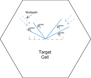
where D𝐷D is the antenna spacing and λ𝜆\lambda is the signal wavelength. Let Q𝑄Q denote the number of clusters. Let [θqmin,θqmax]superscriptsubscript𝜃𝑞minsuperscriptsubscript𝜃𝑞max[\theta_{q}^{\text{min}},\theta_{q}^{\text{max}}] denote the interval of AOAs for the q𝑞q-th cluster of desired paths in the [0,π]0𝜋[0,\pi] interval. See an illustration in Fig. 1 for Q=2𝑄2Q=2.

Refer to caption
Figure 1: Desired channel composed of Q=2𝑄2Q=2 clusters of multipath.

For a uniform linear array, we have the following proposition in the massive MIMO regime:

Proposition 1.

The rank of channel covariance matrix 𝐑𝐑{{\mathbf{R}}} satisfies:

rank(𝐑)Md, when M is sufficiently large ,rank𝐑𝑀𝑑 when 𝑀 is sufficiently large \frac{\operatorname{rank}({{\mathbf{R}}})}{M}\leqslant{d},\text{ when }M\text{ is sufficiently large },

where d𝑑{d} is defined as

dmin(1,q=1Q(cos(θqmin)cos(θqmax))Dλ).𝑑1superscriptsubscript𝑞1𝑄superscriptsubscript𝜃𝑞minsuperscriptsubscript𝜃𝑞max𝐷𝜆{d}\triangleq\min(1,\sum\limits_{q=1}^{Q}{\left({\cos(\theta_{q}^{{\text{min}}})-\cos(\theta_{q}^{{\text{max}}})}\right)}\frac{D}{\lambda}).

Proof: The channel can be seen as the sum of elementary channels each of which corresponds to one separate clusters. Then 𝐑𝐑{\mathbf{R}} can be decomposed into a sum of covariances over these clusters. Since the clusters are separated, the signal subspaces of the corresponding covariances are orthogonal and therefore their dimensions add up. Then based on [10] Lemma 1, the proof of Proposition 1 can be readily obtained.   

Now define the total set of AOAs of the desired channel as

θ¯dq=1Q[θqmin,θqmax],subscript¯𝜃𝑑superscriptsubscript𝑞1𝑄superscriptsubscript𝜃𝑞minsuperscriptsubscript𝜃𝑞max\overline{\theta}_{d}\triangleq\cup_{q=1}^{Q}[\theta_{q}^{\text{min}},\theta_{q}^{\text{max}}], (7)

so that the probability density function (PDF) pd(θ)subscript𝑝𝑑𝜃p_{d}(\theta) of the desired AOA satisfies pd(θ)>0subscript𝑝𝑑𝜃0p_{d}(\theta)>0 if θθ¯d𝜃subscript¯𝜃𝑑\theta\in\overline{\theta}_{d} and pd(θ)=0subscript𝑝𝑑𝜃0p_{d}(\theta)=0 if θθ¯d𝜃subscript¯𝜃𝑑\theta\notin\overline{\theta}_{d}. In the same way, the PDF of all interference AOAs satisfies pi(θ)>0subscript𝑝𝑖𝜃0p_{i}(\theta)>0 if θθ¯i𝜃subscript¯𝜃𝑖\theta\in\overline{\theta}_{i} and pi(θ)=0subscript𝑝𝑖𝜃0p_{i}(\theta)=0 otherwise, where θ¯isubscript¯𝜃𝑖\overline{\theta}_{i} is the union of all possible interference AOAs. We have the following result for the massive uniform array:

Corollary 1.

if Dλ/2𝐷𝜆2D\leq\lambda/2 and θ¯dθ¯i=subscript¯𝜃𝑑subscript¯𝜃𝑖\overline{\theta}_{d}\cap\overline{\theta}_{i}=\emptyset, then the MMSE estimate of (4) satisfies:

limM𝐡^1=𝐡^1no int.subscript𝑀subscript^𝐡1superscriptsubscript^𝐡1no int\mathop{\lim}\limits_{M\to\infty}{{\mathbf{\widehat{h}}}_{1}}={\mathbf{\widehat{h}}}_{1}^{{\text{no int}}}. (8)

Proof: It can be shown that from [10] Lemma 2, condition (5) will be fulfilled as long as interfering AOAs do not overlap with any of the clusters for the desired channel, in which case if we analyze the received signal using eigen-value decomposition, we can find the interference disappears asymptotically because of its orthogonality with the signal space of desired channel covariance. (8) is obtained in the same way as [10]. As a result we omit the detailed proof in this paper.   

II-B2 Random Arrays

Tightly calibrated arrays with uniform spacing are hard to realize in practice. An interesting question is whether the above results carry on to the setting of linear arrays with random antenna placement. To study this case, we consider a set of antennas randomly located over a line, and spanning a total aperture of 𝒟𝒟\mathcal{D} meters. We investigate the extended array and 𝒟𝒟\mathcal{D} is allowed to grow with M𝑀M.

In this case, an elementary path coming from an angle θ𝜃\theta can be represented via the corresponding array response vector as:

𝐚(θ)[ej2πd1λcos(θ)ej2πdMλcos(θ)],𝐚𝜃delimited-[]superscript𝑒𝑗2𝜋subscript𝑑1𝜆𝜃missing-subexpressionmissing-subexpressionmissing-subexpressionmissing-subexpressionmissing-subexpressionmissing-subexpressionmissing-subexpressionmissing-subexpressionmissing-subexpressionmissing-subexpressionmissing-subexpressionmissing-subexpressionmissing-subexpressionmissing-subexpressionmissing-subexpressionmissing-subexpressionmissing-subexpressionmissing-subexpressionmissing-subexpressionmissing-subexpressionmissing-subexpressionmissing-subexpressionmissing-subexpressionmissing-subexpressionmissing-subexpressionmissing-subexpressionmissing-subexpressionmissing-subexpressionmissing-subexpressionmissing-subexpressionmissing-subexpressionmissing-subexpressionmissing-subexpressionmissing-subexpressionmissing-subexpressionmissing-subexpressionmissing-subexpressionmissing-subexpressionsuperscript𝑒𝑗2𝜋subscript𝑑𝑀𝜆𝜃missing-subexpressionmissing-subexpressionmissing-subexpressionmissing-subexpressionmissing-subexpressionmissing-subexpressionmissing-subexpressionmissing-subexpressionmissing-subexpressionmissing-subexpressionmissing-subexpressionmissing-subexpressionmissing-subexpressionmissing-subexpressionmissing-subexpressionmissing-subexpressionmissing-subexpressionmissing-subexpressionmissing-subexpression{\mathbf{a}}({\theta})\triangleq\left[{\begin{array}[]{*{20}{c}}{{e^{-j2\pi\frac{d_{1}}{\lambda}\cos({\theta})}}}\\ \vdots\\ {{e^{-j2\pi\frac{d_{M}}{\lambda}\cos({\theta})}}}\end{array}}\right], (9)

where the position of the m𝑚m-th antenna333Note that antenna ordering has no impact on our results. (1mM1𝑚𝑀1\leq{m}\leq M), dmsubscript𝑑𝑚d_{m}, follows a uniform distribution, i.e., dm𝒰(0,𝒟)similar-tosubscript𝑑𝑚𝒰0𝒟d_{m}\sim\mathcal{U}(0,\mathcal{D}). The PDF of AOA θ𝜃\theta for the desired paths is non-zero only when θθ¯d𝜃subscript¯𝜃𝑑\theta\in\overline{\theta}_{d}, as in section II-B1. Define the average antenna spacing D¯𝒟/M¯𝐷𝒟𝑀\overline{D}\triangleq\mathcal{D}/M. Assuming the aperture of antenna array 𝒟𝒟\mathcal{D} is increasing linearly with M𝑀M, i.e., D¯¯𝐷\overline{D} is constant, we now have the extended results on the low-dimensional property:

Proposition 2.

Define

𝜶(x)𝜶𝑥\displaystyle\boldsymbol{\alpha}(x) [ej2πd1λx,,ej2πdMλx]Tabsentsuperscriptsuperscript𝑒𝑗2𝜋subscript𝑑1𝜆𝑥superscript𝑒𝑗2𝜋subscript𝑑𝑀𝜆𝑥𝑇\displaystyle\triangleq\left[{{e^{-j2\pi\frac{d_{1}}{\lambda}x}}},\cdots,{{e^{-j2\pi\frac{d_{M}}{\lambda}x}}}\right]^{T}
\displaystyle\mathcal{B} span{𝜶(x),x[b1,b2]}absentspan𝜶𝑥𝑥subscript𝑏1subscript𝑏2\displaystyle\triangleq\operatorname{span}\{\boldsymbol{\alpha}(x),x\in[{b_{1}},{b_{2}}]\}
𝒞𝒞\displaystyle\mathcal{C} span{𝜶(x),xb¯},absentspan𝜶𝑥𝑥¯𝑏\displaystyle\triangleq\operatorname{span}\{{\boldsymbol{\alpha}}(x),x\in\overline{b}\},

where b1,b2[1,1]subscript𝑏1subscript𝑏211{b_{1}},{b_{2}}\in[-1,1], b¯q=1Q[bqmin,bqmax]¯𝑏superscriptsubscript𝑞1𝑄superscriptsubscript𝑏𝑞minsuperscriptsubscript𝑏𝑞max\overline{b}\triangleq\cup_{q=1}^{Q}[b_{q}^{\text{min}},b_{q}^{\text{max}}], and bqminsuperscriptsubscript𝑏𝑞minb_{q}^{\text{min}}, bqmaxsuperscriptsubscript𝑏𝑞maxb_{q}^{\text{max}} are values such that

1b1min<b1max<<bqmin<bqmax<<bQmin<bQmax11superscriptsubscript𝑏1minsuperscriptsubscript𝑏1maxsuperscriptsubscript𝑏𝑞minsuperscriptsubscript𝑏𝑞maxsuperscriptsubscript𝑏𝑄minsuperscriptsubscript𝑏𝑄max1-1\leqslant b_{1}^{{\text{min}}}<b_{1}^{{\text{max}}}<\cdots<b_{q}^{{\text{min}}}<b_{q}^{{\text{max}}}<\cdots<b_{Q}^{{\text{min}}}<b_{Q}^{{\text{max}}}\leqslant 1

then we have

  • dim{}(b2b1)MD¯/λ+o(M)dimensionsubscript𝑏2subscript𝑏1𝑀¯𝐷𝜆𝑜𝑀\dim\{\mathcal{B}\}\leq{({b_{2}}-{b_{1}})M\overline{D}/\lambda}+o(M)

  • dim{𝒞}q=1Q(bqmaxbqmin)MD¯/λ+o(M)dimension𝒞superscriptsubscript𝑞1𝑄superscriptsubscript𝑏𝑞maxsuperscriptsubscript𝑏𝑞min𝑀¯𝐷𝜆𝑜𝑀\dim\{\mathcal{C}\}\leq\sum\nolimits_{q=1}^{Q}{\left({b_{q}^{{\text{max}}}-b_{q}^{{\text{min}}}}\right)M\overline{D}/\lambda}+o(M)

Proof: See Appendix -A.   

Proposition 2 indicates the dimensions spanned in massive MIMO regime by elementary paths for (i) single cluster of AOA, and (ii) multiple disjoint clusters of AOA, respectively. The following result now directly generalizes Proposition 1 to random arrays.

Proposition 3.

With a bounded support of AOAs θ¯dsubscript¯𝜃𝑑\overline{\theta}_{d} as in (7), the rank of channel covariance matrix 𝐑𝐑{{\mathbf{R}}} satisfies:

rank(𝐑)q=1Q(cos(θqmin)cos(θqmax))MD¯λ+o(M),rank𝐑superscriptsubscript𝑞1𝑄superscriptsubscript𝜃𝑞minsuperscriptsubscript𝜃𝑞max𝑀¯𝐷𝜆𝑜𝑀{\operatorname{rank}({{\mathbf{R}}})}\leq{\sum\limits_{q=1}^{Q}{\left({\cos(\theta_{q}^{{\text{min}}})-\cos(\theta_{q}^{{\text{max}}})}\right)}\frac{M\overline{D}}{\lambda}}+o(M), (10)

Proof: We can readily obtain this result by replacing x𝑥x with cos(θ)𝜃\cos(\theta) in Proposition 2.   

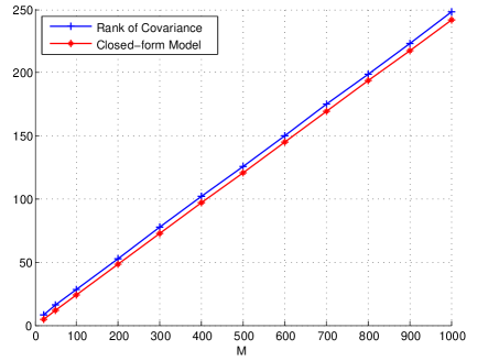
This result above suggests that the low-dimensional feature of signal subspaces in massive MIMO is not critically linked to the Fourier structure of the steering vectors. Furthermore, it should be noted that the above upper bound is actually very tight for large M𝑀M, as witnessed from the simulation in Fig. 2, where we take Q=1,D¯=λ/2formulae-sequence𝑄1¯𝐷𝜆2Q=1,\overline{D}=\lambda/2 for example. The AOA spread is 40 degrees, and the closed form model refers to

f(M)q=1Q(cos(θqmin)cos(θqmax))MD¯λ.𝑓𝑀superscriptsubscript𝑞1𝑄superscriptsubscript𝜃𝑞minsuperscriptsubscript𝜃𝑞max𝑀¯𝐷𝜆f(M)\triangleq{\sum\limits_{q=1}^{Q}{\left({\cos(\theta_{q}^{{\text{min}}})-\cos(\theta_{q}^{{\text{max}}})}\right)}\frac{M\overline{D}}{\lambda}}.

We can observe that rank(𝐑)rank𝐑{\operatorname{rank}({{\mathbf{R}}})} is well approximated by f(M)𝑓𝑀f(M).

Refer to caption
Figure 2: Closed-form rank model for the channel covariance vs. actual rank.

Proposition 3 and Fig. 2 suggest that a property of rank additivity holds for multiple disjoint clusters of AOAs in the massive MIMO regime, i.e. for M+.𝑀M\rightarrow+\infty. In the following proposition we extend the results of Corollary 1 to the case of random arrays under the weaker assumption of rank additivity for the covariance matrices of the desired and interference channels.

Proposition 4.

Let 𝐑dsubscript𝐑𝑑\mathbf{R}_{d} be the covariance matrix of desired channel and 𝐑isubscript𝐑𝑖\mathbf{R}_{i} be the covariance of the sum of all interference channels. If 𝐑dsubscript𝐑𝑑\mathbf{R}_{d} and 𝐑isubscript𝐑𝑖\mathbf{R}_{i} satisfy the following rank additivity property

rank(𝐑d+𝐑i)=rank(𝐑d)+rank(𝐑i),ranksubscript𝐑𝑑subscript𝐑𝑖ranksubscript𝐑𝑑ranksubscript𝐑𝑖\mathrm{rank}(\mathbf{R}_{d}+\mathbf{R}_{i})=\mathrm{rank}(\mathbf{R}_{d})+\mathrm{rank}(\mathbf{R}_{i}),

then in the high SNR regime, the linear MMSE estimate of the desired channel is error free, or, in other words, its error covariance matrix 𝐂esubscript𝐂𝑒\mathbf{C}_{e} vanishes.

Proof: In the case of absence of white Gaussian noise, i.e. σn2=0,superscriptsubscript𝜎𝑛20\sigma_{n}^{2}=0, and rank deficient signal and interference covariance matrices, the error covariance matrix of linear MMSE estimator [20] can be generalized as

𝐂e=𝐑d𝐑d(𝐑d+𝐑i)𝐑dsubscript𝐂𝑒subscript𝐑𝑑subscript𝐑𝑑superscriptsubscript𝐑𝑑subscript𝐑𝑖subscript𝐑𝑑\mathbf{C}_{e}=\mathbf{R}_{d}-\mathbf{R}_{d}(\mathbf{R}_{d}+\mathbf{R}_{i})^{{\dagger}}\mathbf{R}_{d} (11)

where ()superscript(\cdot)^{{\dagger}} denotes the Moore-Penrose generalized inverse of the matrix argument. Let us denote by 𝐑x=𝐔x𝚺x𝐔xH,subscript𝐑𝑥subscript𝐔𝑥subscript𝚺𝑥superscriptsubscript𝐔𝑥𝐻\mathbf{R}_{x}=\mathbf{U}_{x}\boldsymbol{\Sigma}_{x}\mathbf{U}_{x}^{H}, with x{d,e},𝑥𝑑𝑒x\in\{d,e\}, 𝐔xsubscript𝐔𝑥\mathbf{U}_{x} unitary matrix, and 𝚺xsubscript𝚺𝑥\boldsymbol{\Sigma}_{x} diagonal matrix, the eigenvalue decomposition of the Hermitian matrix 𝐑x.subscript𝐑𝑥\mathbf{R}_{x}. Then, 𝐑x=𝐔x𝚺x𝐔xH,subscriptsuperscript𝐑𝑥subscript𝐔𝑥superscriptsubscript𝚺𝑥superscriptsubscript𝐔𝑥𝐻\mathbf{R}^{{\dagger}}_{x}=\mathbf{U}_{x}\boldsymbol{\Sigma}_{x}^{{\dagger}}\mathbf{U}_{x}^{H}, where the elements i,j𝑖𝑗i,j of the matrix 𝚺xsuperscriptsubscript𝚺𝑥\boldsymbol{\Sigma}_{x}^{{\dagger}} are given by

𝚺x,ij={𝚺x,ii1,if i=j and 𝚺x,ii0;0,otherwise.superscriptsubscript𝚺𝑥𝑖𝑗casessuperscriptsubscript𝚺𝑥𝑖𝑖1if i=j and 𝚺x,ii0;0otherwise.\boldsymbol{\Sigma}_{x,ij}^{{\dagger}}=\left\{\begin{array}[]{ll}\boldsymbol{\Sigma}_{x,ii}^{-1},&\hbox{if $i=j$ and $\boldsymbol{\Sigma}_{x,ii}\neq 0$;}\\ 0,&\hbox{otherwise.}\end{array}\right.

Additionally, 𝐔~xsubscript~𝐔𝑥\widetilde{\mathbf{U}}_{x} denotes the column space of 𝐑xsubscript𝐑𝑥\mathbf{R}_{x} and 𝚺~xsubscript~𝚺𝑥\widetilde{\boldsymbol{\Sigma}}_{x} the corresponding nonzero eigenvalues such that 𝐑x=𝐔~x𝚺~x𝐔~xH.subscript𝐑𝑥subscript~𝐔𝑥subscript~𝚺𝑥superscriptsubscript~𝐔𝑥𝐻\mathbf{R}_{x}=\widetilde{\mathbf{U}}_{x}\widetilde{\boldsymbol{\Sigma}}_{x}\widetilde{\mathbf{U}}_{x}^{H}. Then, under the assumption of rank additivity of the covariance matrices 𝐑dsubscript𝐑𝑑\mathbf{R}_{d} and 𝐑isubscript𝐑𝑖\mathbf{R}_{i}, the theorem on the Moore-Penrose generalized inverse for sum of matrices in [21] yields

(𝐑d+𝐑i)=(𝐈𝐒)𝐑d(𝐈𝐓)+𝐒𝐑i𝐓,superscriptsubscript𝐑𝑑subscript𝐑𝑖𝐈superscript𝐒superscriptsubscript𝐑𝑑𝐈superscript𝐓superscript𝐒superscriptsubscript𝐑𝑖superscript𝐓(\mathbf{R}_{d}+\mathbf{R}_{i})^{{\dagger}}=(\mathbf{I}-\mathbf{S}^{{\dagger}})\mathbf{R}_{d}^{{\dagger}}(\mathbf{I}-\mathbf{T}^{{\dagger}})+\mathbf{S}^{{\dagger}}\mathbf{R}_{i}^{{\dagger}}\mathbf{T}^{{\dagger}}, (12)

where 𝐒=𝐔~i𝐔~iH(𝐈𝐔~d𝐔~dH)𝐒subscript~𝐔𝑖superscriptsubscript~𝐔𝑖𝐻𝐈subscript~𝐔𝑑superscriptsubscript~𝐔𝑑𝐻\mathbf{S}=\widetilde{\mathbf{U}}_{i}\widetilde{\mathbf{U}}_{i}^{H}(\mathbf{I}-\widetilde{\mathbf{U}}_{d}\widetilde{\mathbf{U}}_{d}^{H}) and 𝐓=(𝐈𝐔~d𝐔~dH)𝐔~i𝐔~iH.𝐓𝐈subscript~𝐔𝑑superscriptsubscript~𝐔𝑑𝐻subscript~𝐔𝑖superscriptsubscript~𝐔𝑖𝐻\mathbf{T}=(\mathbf{I}-\widetilde{\mathbf{U}}_{d}\widetilde{\mathbf{U}}_{d}^{H})\widetilde{\mathbf{U}}_{i}\widetilde{\mathbf{U}}_{i}^{H}.

Let us observe that

𝐓𝐑d=𝟎 and 𝐑d𝐒=𝟎.formulae-sequencesuperscript𝐓subscript𝐑𝑑0 and subscript𝐑𝑑superscript𝐒0\mathbf{T}^{{\dagger}}\mathbf{R}_{d}=\mathbf{0}\quad\text{ and }\quad\mathbf{R}_{d}\mathbf{S}^{{\dagger}}=\mathbf{0}. (13)

We focus on the first equality. The proof of the second equation follows along the same line. By appealing to the mixed type reverse order laws of the r×s𝑟𝑠r\times s matrix 𝐀𝐀\mathbf{A} and the s×t𝑠𝑡s\times t matrix 𝐁𝐁\mathbf{B} in [22]

(𝐀𝐁)=𝐁H(𝐀H𝐀𝐁𝐁H)𝐀H,superscript𝐀𝐁superscript𝐁𝐻superscriptsuperscript𝐀𝐻superscript𝐀𝐁𝐁𝐻superscript𝐀𝐻(\mathbf{A}\mathbf{B})^{{\dagger}}=\mathbf{B}^{H}(\mathbf{A}^{H}\mathbf{A}\mathbf{B}\mathbf{B}^{H})^{{\dagger}}\mathbf{A}^{H},

𝐓superscript𝐓\mathbf{T}^{{\dagger}} can be rewritten as

𝐓superscript𝐓\displaystyle\mathbf{T}^{{\dagger}} =𝐔~i𝐔~iH[(𝐈𝐔~d𝐔~dH)𝐔~i𝐔~iH](𝐈𝐔~d𝐔~dH)absentsubscript~𝐔𝑖superscriptsubscript~𝐔𝑖𝐻superscriptdelimited-[]𝐈subscript~𝐔𝑑superscriptsubscript~𝐔𝑑𝐻subscript~𝐔𝑖superscriptsubscript~𝐔𝑖𝐻𝐈subscript~𝐔𝑑superscriptsubscript~𝐔𝑑𝐻\displaystyle=\widetilde{\mathbf{U}}_{i}\widetilde{\mathbf{U}}_{i}^{H}\left[(\mathbf{I}-\widetilde{\mathbf{U}}_{d}\widetilde{\mathbf{U}}_{d}^{H})\widetilde{\mathbf{U}}_{i}\widetilde{\mathbf{U}}_{i}^{H}\right]^{{\dagger}}(\mathbf{I}-\widetilde{\mathbf{U}}_{d}\widetilde{\mathbf{U}}_{d}^{H})
=𝐔~i𝐔~iH𝐓(𝐈𝐔~d𝐔~dH).absentsubscript~𝐔𝑖superscriptsubscript~𝐔𝑖𝐻superscript𝐓𝐈subscript~𝐔𝑑superscriptsubscript~𝐔𝑑𝐻\displaystyle=\widetilde{\mathbf{U}}_{i}\widetilde{\mathbf{U}}_{i}^{H}\mathbf{T}^{{\dagger}}(\mathbf{I}-\widetilde{\mathbf{U}}_{d}\widetilde{\mathbf{U}}_{d}^{H}).

The first equality is obtained utilizing the fact that the matrices 𝐔~i𝐔~iHsubscript~𝐔𝑖superscriptsubscript~𝐔𝑖𝐻\widetilde{\mathbf{U}}_{i}\widetilde{\mathbf{U}}_{i}^{H} and (𝐈𝐔~d𝐔~dH)𝐈subscript~𝐔𝑑superscriptsubscript~𝐔𝑑𝐻(\mathbf{I}-\widetilde{\mathbf{U}}_{d}\widetilde{\mathbf{U}}_{d}^{H}) are orthogonal projectors and thus idempotent. Then,

𝐓𝐑d=𝐔~i𝐔~iH𝐓(𝐈𝐔~d𝐔~dH)𝐔~d𝚺~d𝐔~dH=𝟎.superscript𝐓subscript𝐑𝑑subscript~𝐔𝑖superscriptsubscript~𝐔𝑖𝐻superscript𝐓𝐈subscript~𝐔𝑑superscriptsubscript~𝐔𝑑𝐻subscript~𝐔𝑑subscript~𝚺𝑑superscriptsubscript~𝐔𝑑𝐻0\mathbf{T}^{{\dagger}}\mathbf{R}_{d}=\widetilde{\mathbf{U}}_{i}\widetilde{\mathbf{U}}_{i}^{H}\mathbf{T}^{{\dagger}}(\mathbf{I}-\widetilde{\mathbf{U}}_{d}\widetilde{\mathbf{U}}_{d}^{H})\widetilde{\mathbf{U}}_{d}\widetilde{\boldsymbol{\Sigma}}_{d}\widetilde{\mathbf{U}}_{d}^{H}=\mathbf{0}.

Finally, substituting (12) into (11) and accounting for orthogonality in (13)

𝐂esubscript𝐂𝑒\displaystyle\mathbf{C}_{e} =𝐑d𝐑d[(𝐈𝐒)𝐑d(𝐈𝐓)+𝐒𝐑i𝐓]𝐑dabsentsubscript𝐑𝑑subscript𝐑𝑑delimited-[]𝐈superscript𝐒superscriptsubscript𝐑𝑑𝐈superscript𝐓superscript𝐒superscriptsubscript𝐑𝑖superscript𝐓subscript𝐑𝑑\displaystyle=\mathbf{R}_{d}-\mathbf{R}_{d}\left[(\mathbf{I}-\mathbf{S}^{{\dagger}})\mathbf{R}_{d}^{{\dagger}}(\mathbf{I}-\mathbf{T}^{{\dagger}})+\mathbf{S}^{{\dagger}}\mathbf{R}_{i}^{{\dagger}}\mathbf{T}^{{\dagger}}\right]\mathbf{R}_{d}
=𝐑d𝐑d𝐑d𝐑d=𝟎.absentsubscript𝐑𝑑subscript𝐑𝑑superscriptsubscript𝐑𝑑subscript𝐑𝑑0\displaystyle=\mathbf{R}_{d}-\mathbf{R}_{d}\mathbf{R}_{d}^{{\dagger}}\mathbf{R}_{d}=\mathbf{0}.

In the last equality we use one of the fundamental relations defining the Moore-Penrose generalized inverse.   

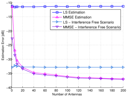
According to Proposition 3, the rank additivity condition is in general satisfied when the AOA support of desired channel and that of interference channels span disjoint region of spaces, i.e., θ¯dθ¯i=subscript¯𝜃𝑑subscript¯𝜃𝑖\overline{\theta}_{d}\cap\overline{\theta}_{i}=\emptyset. This property can be exploited in pilot decontamination or interference rejection. Fig. 3 shows the channel estimation performance in the presence of contaminating pilots. In the simulation, we consider a 2-cell network. Each cell has one single-antenna user who uses identical pilot sequence. The mean squared error (MSE) of uplink channel estimation is shown. The simulation suggests that the MMSE channel estimator is able to rid itself from pilot contamination effects as the number of antennas is (even moderately) large, which verifies Proposition 4.
Refer to caption
Figure 3: Channel estimation performance vs. M𝑀M, D¯=λ/2¯𝐷𝜆2\overline{D}=\lambda/2, 2-cell network, angle spread 30 degrees, θ¯dθ¯i=subscript¯𝜃𝑑subscript¯𝜃𝑖\overline{\theta}_{d}\cap\overline{\theta}_{i}=\emptyset, cell-edge SNR is 20dB. We compare the standard Least Squares (LS) to MMSE estimators, in interference and interference-free scenarios.

III Finite Rank Model in Distributed Arrays

We now turn to another popular form of large scale antenna regime, often referred to in the literature as distributed antenna systems. In such a setting, a virtual base station is deployed having its M𝑀M antennas scattered throughout the cell.444For ease of exposition we temporarily consider a single cell setting in this section, i.e., B=1𝐵1B=1. However simulation is also done later in a multi-cell scenario. We consider again the uplink in which joint combining across all BS antennas is assumed possible. The M𝑀M base station antennas are assumed uniformly and randomly located in a fixed size network, serving single-antenna users. M𝑀M is allowed to grow large giving rise to a so-called dense network. Our model assumes a disk-shaped cell of radius L𝐿L, although simulation and intuition confirm that the actual shape of the cell’s boundary is irrelevant to the main result.

III-A Channel Model

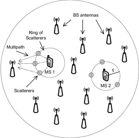
In order to facilitate the analysis, we adopt the one-ring model [14, 15] where users are surrounded by a ring of P𝑃P local scatterers (see Fig. 4) located r𝑟r meters away from the user. The positions of the scatterers are considered to follow a uniform distribution on the ring. In the one-ring model, the propagation from user to base is assumed to follow P𝑃P paths (hereafter referred to as scattering paths), where each path p𝑝p bounces once on the p𝑝p-th scatterer before reaching all M𝑀M destinations.555Note that this model assumes the BS antennas are high enough above clutter so that there is no local scattering around the BS antennas.

Hence, the path length from user k𝑘k to the m𝑚m-th antenna via the p𝑝p-th path is r+dkpm𝑟subscript𝑑𝑘𝑝𝑚r+d_{kpm}, where dkpmsubscript𝑑𝑘𝑝𝑚d_{kpm} is the distance between the p𝑝p-th scatterer of the k𝑘k-th user and the m𝑚m-th BS antenna. The path loss of the p𝑝p-th scattering path is modeled by:

βkpm=α(dkpm+r)γ,subscript𝛽𝑘𝑝𝑚𝛼superscriptsubscript𝑑𝑘𝑝𝑚𝑟𝛾{\beta_{kpm}}=\frac{\alpha}{{{(d_{kpm}+r)}^{\gamma}}}, (14)

where α𝛼\alpha is a constant that can be computed based on desired cell-edge SNR, and γ𝛾\gamma is the path loss exponent. We scale the amplitude of each path by P𝑃\sqrt{P}. The channel between user k𝑘k and all BS antennas is given by:

𝐡k1Pp=1P𝐡kp,subscript𝐡𝑘1𝑃superscriptsubscript𝑝1𝑃subscript𝐡𝑘𝑝{\mathbf{h}_{k}}\triangleq\frac{1}{\sqrt{P}}\sum\limits_{p=1}^{P}{{{\mathbf{h}}_{kp}}}, (15)

where 𝐡kpsubscript𝐡𝑘𝑝{\mathbf{h}_{kp}} is the p𝑝p-th scattering path vector channel between user k𝑘k and all base stations:

𝐡kp[βkp1ej2πdkp1+rλβkpMej2πdkpM+rλ]ejφkp,subscript𝐡𝑘𝑝delimited-[]subscript𝛽𝑘𝑝1superscript𝑒𝑗2𝜋subscript𝑑𝑘𝑝1𝑟𝜆missing-subexpressionmissing-subexpressionmissing-subexpressionmissing-subexpressionmissing-subexpressionmissing-subexpressionmissing-subexpressionmissing-subexpressionmissing-subexpressionmissing-subexpressionmissing-subexpressionmissing-subexpressionmissing-subexpressionmissing-subexpressionmissing-subexpressionmissing-subexpressionmissing-subexpressionmissing-subexpressionmissing-subexpressionmissing-subexpressionmissing-subexpressionmissing-subexpressionmissing-subexpressionmissing-subexpressionmissing-subexpressionmissing-subexpressionmissing-subexpressionmissing-subexpressionmissing-subexpressionmissing-subexpressionmissing-subexpressionmissing-subexpressionmissing-subexpressionmissing-subexpressionmissing-subexpressionmissing-subexpressionmissing-subexpressionmissing-subexpressionsubscript𝛽𝑘𝑝𝑀superscript𝑒𝑗2𝜋subscript𝑑𝑘𝑝𝑀𝑟𝜆missing-subexpressionmissing-subexpressionmissing-subexpressionmissing-subexpressionmissing-subexpressionmissing-subexpressionmissing-subexpressionmissing-subexpressionmissing-subexpressionmissing-subexpressionmissing-subexpressionmissing-subexpressionmissing-subexpressionmissing-subexpressionmissing-subexpressionmissing-subexpressionmissing-subexpressionmissing-subexpressionmissing-subexpressionsuperscript𝑒𝑗subscript𝜑𝑘𝑝{\mathbf{h}_{kp}}\triangleq\left[{\begin{array}[]{*{20}{c}}{\sqrt{\beta_{kp1}}{e^{-j2\pi\frac{d_{kp1}+r}{\lambda}}}}\\ \vdots\\ {\sqrt{\beta_{kpM}}{e^{-j2\pi\frac{d_{kpM}+r}{\lambda}}}}\end{array}}\right]e^{j\varphi_{kp}}, (16)

where ejφkpsuperscript𝑒𝑗subscript𝜑𝑘𝑝e^{j\varphi_{kp}} denotes the random common phase of that scattering path vector due to possible random perturbations of the user location around the ring center or the phase shift due to the reflection on the scatterer. φkpsubscript𝜑𝑘𝑝\varphi_{kp} is assumed i.i.d. and uniformly distributed between 0 to 2π2𝜋2\pi.

Refer to caption
Figure 4: The distributed large-scale antenna setting with a one-ring model.

III-B A Low-rank Model for Distributed Arrays

We have shown in section II-B the low-dimension property for linear antenna array systems. In attacking this problem it is important to distinguish the rank reduction effect due to path loss from the intrinsic finite-rank behavior of the large antenna channel covariance in an equal path loss regime. In fact, in an extended network (i.e. where some base station antennas can be arbitrarily far from some users), the signal of any given user will be received over only a limited number of antennas in its vicinity, thereby effectively limiting the channel rank to the size of this neighborhood. To circumvent this problem, we consider below a (dense) network where the path loss terms are set artificially to be all equal (to one) and study the finite-rankness under such conditions. In this model, the channel covariance is defined as 𝐑𝔼{𝐡𝐡H}𝐑𝔼superscript𝐡𝐡𝐻{{\mathbf{R}}}\triangleq\mathbb{E}\{{{{\mathbf{h}}}{\mathbf{h}}^{H}}\} where the expectation is taken over the random positions of the scatterers on the ring. Note that our analysis indicates that a randomization over the user’s location inside the scattering’s disk would produce an identical upper bound on the rank.

Theorem 1.

The rank of the channel covariance matrix for a distributed antenna system satisfies:

rank(𝐑)4πrλ+o(r).rank𝐑4𝜋𝑟𝜆𝑜𝑟{\text{rank}({\mathbf{R}})}\leq\frac{4\pi r}{\lambda}+o(r). (17)

Proof: See Appendix -B.   

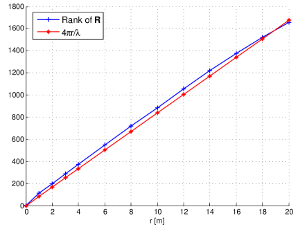
In reality we show below that the right hand side of (17) is a very close approximation of the actual rank, which is defined as the number of eigenvalues of 𝐑𝐑\mathbf{R} which are greater than a prescribed threshold (in our simulations it is taken to be 10e-5). Theorem 1 shows a linear dependency of the rank on the size of the scattering ring. When r𝑟r increases, the richer scattering environment expands the dimension of signal space.
Refer to caption
Figure 5: Rank vs. r𝑟r, M=2000𝑀2000M=2000, λ𝜆\lambda = 0.15m, L=500𝐿500L=500m.

Fig. 5 shows the behavior of the covariance rank with respect to the scattering radius r𝑟r. We can see the rank scales linearly with the slope 4π/λ4𝜋𝜆4\pi/\lambda. However because of the finite number of antennas the rank will finally saturate towards M𝑀M when r𝑟r keeps increasing.

IV Spatial Interference Filtering

We are now interested in characterizing the orthogonality (or correlation) between any two user channel vectors as a function of inter-user distance, the wavelength and the scattering radius r𝑟r, in the large M𝑀M limit, as this will provide a measure of interference rejection capability for the distributed antenna systems. In the following we will investigate two interference filtering schemes: 1) the simplistic matched filtering, 2) a subspace projection filtering.

IV-A Performance of Interference Filtering Using Matched Filter

We start with analyzing the channel correlation between two users who interfere each other. We point out two distinct regimes, depending on whether the inter-user distance is small or large.

IV-A1 Closely Spaced Users

Closely spaced users are defined by the fact that the distance between user 1’s and user 2’s scatterers is small enough compared with the distance between scatterers and receiving antennas so that we can consider planar wavefronts. We first examine the correlation between any two scattering paths for user 1 and user 2, corresponding to user 1’s p𝑝p-th scatterer and user 2’s q𝑞q-th scatterer, with a distance Dpqsubscript𝐷𝑝𝑞D_{pq}.

Proposition 5.

For Dpqsubscript𝐷𝑝𝑞D_{pq} small enough that the two scatterers are located in the same planar wavefront region, we have

limM|𝐡2qH𝐡1p||𝐡1p||𝐡2q||J0(2πDpqλ)|,subscript𝑀superscriptsubscript𝐡2𝑞𝐻subscript𝐡1𝑝subscript𝐡1𝑝subscript𝐡2𝑞subscript𝐽02𝜋subscript𝐷𝑝𝑞𝜆\mathop{\lim}\limits_{M\to\infty}\frac{{\left|{{\mathbf{h}}_{2q}^{H}{{\mathbf{h}}_{1p}}}\right|}}{{\left|{{{\mathbf{h}}_{1p}}}\right|\left|{{{\mathbf{h}}_{2q}}}\right|}}\approx\left|{{J_{0}}\left(\frac{{2\pi{D_{pq}}}}{\lambda}\right)}\right|, (18)

where J0subscript𝐽0{J_{0}} is the zero-order Bessel function of the first kind.

Proof: See Appendix -C.   

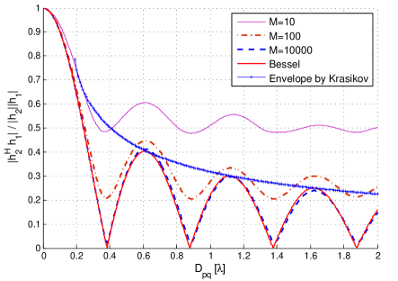
Note that the proof is based on an additional assumption that the path loss between a certain antenna and the two scatterers are approximately equal, i.e., if user 1 and user 2 are concerned, then β2qmβ1pmsubscript𝛽2𝑞𝑚subscript𝛽1𝑝𝑚{\beta_{2qm}}\approx{\beta_{1pm}}. Since the two scatterers are very close and the antenna is much further away, this assumption is reasonable in practice. To visualize Proposition 5, we draw the curves of |𝐡2qH𝐡1p||𝐡1p||𝐡2q|superscriptsubscript𝐡2𝑞𝐻subscript𝐡1𝑝subscript𝐡1𝑝subscript𝐡2𝑞\frac{{\left|{{\mathbf{h}}_{2q}^{H}{{\mathbf{h}}_{1p}}}\right|}}{{\left|{{{\mathbf{h}}_{1p}}}\right|\left|{{{\mathbf{h}}_{2q}}}\right|}} and |J0(2πDpqλ)|subscript𝐽02𝜋subscript𝐷𝑝𝑞𝜆|{J_{0}}(\frac{{2\pi{D_{pq}}}}{\lambda})| in Fig. 6.

Refer to caption
Figure 6: Illustration of Proposition 5.

The curves show that when M𝑀M grows, |𝐡2qH𝐡1p|/|𝐡1p||𝐡2q|superscriptsubscript𝐡2𝑞𝐻subscript𝐡1𝑝subscript𝐡1𝑝subscript𝐡2𝑞{\left|{{\mathbf{h}}_{2q}^{H}{{\mathbf{h}}_{1p}}}\right|}/{\left|{{{\mathbf{h}}_{1p}}}\right|\left|{{{\mathbf{h}}_{2q}}}\right|} gets closer and closer to the Bessel function. The curve named “Envelope by Krasikov” is an upper bound of the Bessel function developed by Krasikov in [23], which will be used in Proposition 6. The interpretation of Proposition 5 is as follows: the highest correlation between two scattering paths is attained when the spacing between the two scatterers is very small. Since the Bessel function reaches its first zero around a spacing of D0=0.38λsubscript𝐷00.38𝜆D_{0}=0.38\lambda, it implies that the users ought to be located at least 2r+D02r2𝑟subscript𝐷02𝑟2r+D_{0}\approx 2r away from each other to allow for a reuse of spectral resources (such as pilots). In practice we would intend to schedule users with additional spacing than just 2r2𝑟2r, according to the side lobes of the Bessel function. Note that our model is similar to Clarke’s model [24], which indicates if the AOA is uniformly distributed from 0 to 2π2𝜋2\pi, the autocorrelation of a moving mobile is a scaled Bessel function.

We use Proposition 5 to derive a lower bound on the signal to interference ratio (SIR) under a simplified system setting with just two users (one desired, one interferer) and a matched filter receiver666With more users, the interference is simply scaled by the number of users. Additionally more advanced receivers could also be exploited.. By computing the expectation over the random BS antenna locations, which is also how we derive the expectation of SIRs and channel correlations in the rest of this section, we obtain the following bound of SIR:

Proposition 6.

Assume perfect channel estimation, closely located users, whose scattering rings do not overlap. The expected SIR at the matched filter output satisfies:

𝔼{SIR}π((4(2π(Du2r)λ)23)323)16(2π(Du2r)λ)220, when M is large,greater-than-or-equivalent-to𝔼SIR𝜋superscript4superscript2𝜋subscript𝐷𝑢2𝑟𝜆2332316superscript2𝜋subscript𝐷𝑢2𝑟𝜆220 when 𝑀 is large,\mathbb{E}\{\text{SIR}\}\gtrsim{{\frac{{\pi\left({{{\left({4{{(\frac{{2\pi{(D_{u}-2r)}}}{\lambda})}^{2}}-3}\right)}^{\frac{3}{2}}}-3}\right)}}{{16{{(\frac{{2\pi{(D_{u}-2r)}}}{\lambda})}^{2}}-20}}}},\text{ when }M\text{ is large,}

where Dusubscript𝐷𝑢D_{u} is the distance between the two users and is assumed to be larger than 3+323λ/(4π)+2r3superscript323𝜆4𝜋2𝑟{{\sqrt{3+{3^{\frac{2}{3}}}}\lambda}}/{{(4\pi)}}+2r.

Proof: When applying matched filter, we have

𝔼{SIR}=𝔼|𝐡1|2|𝐡2|2|𝐡2H𝐡1|2.𝔼SIR𝔼superscriptsubscript𝐡12superscriptsubscript𝐡22superscriptsuperscriptsubscript𝐡2𝐻subscript𝐡12\mathbb{E}\{\text{SIR}\}=\mathbb{E}\frac{{{{\left|{{{\mathbf{h}}_{1}}}\right|}^{2}}{{\left|{{{\mathbf{h}}_{2}}}\right|}^{2}}}}{{{{\left|{{\mathbf{h}}_{2}^{H}{{\mathbf{h}}_{1}}}\right|}^{2}}}}.

Let us recall that the envelope of the Bessel function J0(2πDλ)subscript𝐽02𝜋𝐷𝜆{J_{0}}(\frac{{2\pi D}}{\lambda}) is decreasing with D𝐷D. Thus, the lower bound of SIR is obtained by considering the shortest Dpqsubscript𝐷𝑝𝑞D_{pq}, which gives the worst case correlation. Since DpqDu2rsubscript𝐷𝑝𝑞subscript𝐷𝑢2𝑟D_{pq}\geq D_{u}-2r, we may obtain when M𝑀M is large:

𝔼{SIR}1|J0(2π(Du2r)λ)|2.greater-than-or-equivalent-to𝔼SIR1superscriptsubscript𝐽02𝜋subscript𝐷𝑢2𝑟𝜆2\mathbb{E}\{\text{SIR}\}\gtrsim\frac{1}{\left|{{J_{0}}(\frac{{2\pi{(D_{u}-2r)}}}{\lambda})}\right|^{2}}.

Finally we use an upper bound of the envelope of the Bessel function [23] which has validity when Du2r>3+323λ/(4π)subscript𝐷𝑢2𝑟3superscript323𝜆4𝜋D_{u}-2r>{{\sqrt{3+{3^{\frac{2}{3}}}}\lambda}}/{{(4\pi)}}. The bounding argument of the Bessel function in [23] can directly apply here.   

The above proposition quantifies the rate at which the SIR increases with the inter-user distance, in this case linearly.

IV-A2 Distant Users

We consider the regime in which users are located further away from each other, e.g., many wavelengths away. The planar wavefront assumption no longer holds, making the use of the Bessel function impractical. In this case we are again interested in characterizing the correlation between two scattering paths corresponding to two users, then the correlation between the channel vectors themselves.

We first investigate the behavior of 𝐡2qH𝐡1psuperscriptsubscript𝐡2𝑞𝐻subscript𝐡1𝑝{{\mathbf{h}}_{2q}}^{H}{{\mathbf{h}}_{1p}} for any p𝑝p, q𝑞q:

𝐡2qH𝐡1p=m=1M(h2qmh1pm),superscriptsubscript𝐡2𝑞𝐻subscript𝐡1𝑝superscriptsubscript𝑚1𝑀superscriptsubscript2𝑞𝑚subscript1𝑝𝑚{{\mathbf{h}}_{2q}}^{H}{{\mathbf{h}}_{1p}}=\sum\limits_{m=1}^{M}{\left({h_{2qm}^{*}{h_{1pm}}}\right)}, (19)

where hkpmsubscript𝑘𝑝𝑚h_{kpm} is the channel between the k𝑘k-th user and the m𝑚m-th BS antenna via the p𝑝p-th scatterer:

hkpm=βkpmej2πdkpm+rλejφkp.subscript𝑘𝑝𝑚subscript𝛽𝑘𝑝𝑚superscript𝑒𝑗2𝜋subscript𝑑𝑘𝑝𝑚𝑟𝜆superscript𝑒𝑗subscript𝜑𝑘𝑝h_{kpm}=\sqrt{\beta_{kpm}}{e^{-j2\pi\frac{{{d_{kpm}}+r}}{\lambda}}}e^{j\varphi_{kp}}. (20)

Since the two phases ejφ1psuperscript𝑒𝑗subscript𝜑1𝑝e^{j\varphi_{1p}} and ejφ2qsuperscript𝑒𝑗subscript𝜑2𝑞e^{j\varphi_{2q}} are independent, we have:

𝐄(h2qmh1pm)=0,𝐄superscriptsubscript2𝑞𝑚subscript1𝑝𝑚0\mathbf{E}(h_{2qm}^{*}h_{1pm})=0,

and the variance of h2qmh1pmsuperscriptsubscript2𝑞𝑚subscript1𝑝𝑚h_{2qm}^{*}h_{1pm} is

σ2(Dpq)Var(h2qmh1pm)=𝐄(β2qmβ1pm).superscript𝜎2subscript𝐷𝑝𝑞Varsuperscriptsubscript2𝑞𝑚subscript1𝑝𝑚𝐄subscript𝛽2𝑞𝑚subscript𝛽1𝑝𝑚\sigma^{2}(D_{pq})\triangleq\text{Var}(h_{2qm}^{*}h_{1pm})=\mathbf{E}(\beta_{2qm}\beta_{1pm}). (21)

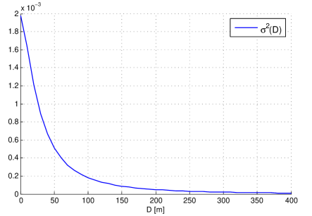
Given the random network model with radius L𝐿L, the path loss correlation can be found by integration over polar coordinates giving the location of the BS antennas. Although a closed-form expression is elusive, we get the following computable expression:

σ2(D)=superscript𝜎2𝐷absent\displaystyle\sigma^{2}(D)=
2απL20L𝑑ρ0πρ(ρ+r)γ(D2+ρ22ρDcos(φ)+r)γ𝑑φ2𝛼𝜋superscript𝐿2superscriptsubscript0𝐿differential-d𝜌superscriptsubscript0𝜋𝜌superscript𝜌𝑟𝛾superscriptsuperscript𝐷2superscript𝜌22𝜌𝐷𝜑𝑟𝛾differential-d𝜑\displaystyle\frac{{2{\alpha}}}{{\pi{L^{2}}}}\int_{0}^{L}{d\rho\int_{0}^{\pi}{\frac{\rho}{{{{\left({\rho+r}\right)}^{\gamma}}{{\left({\sqrt{D^{2}+{\rho^{2}}-2\rho{D}\cos(\varphi)}+r}\right)}^{\gamma}}}}}}d\varphi (22)

One example of the path loss correlation σ2(D)superscript𝜎2𝐷\sigma^{2}(D) is given in Fig. 7, which shows σ2(D)superscript𝜎2𝐷\sigma^{2}(D) is a decreasing function of D𝐷D.

Refer to caption
Figure 7: An illustration of σ2(D)superscript𝜎2𝐷\sigma^{2}(D) with α=107𝛼superscript107\alpha=10^{7}, L=500𝐿500L=500, r=15𝑟15r=15, and γ=2.5.𝛾2.5\gamma=2.5.

We have the following proposition on the distribution of |𝐡2qH𝐡1p|2superscriptsuperscriptsubscript𝐡2𝑞𝐻subscript𝐡1𝑝2|{{\mathbf{h}}_{2q}^{H}{{\mathbf{h}}_{1p}}}|^{2}:

Proposition 7.

Let χ𝜒\chi be a random variable exponentially distributed with parameter λ=2𝜆2\lambda=2. Asymptotically for M+𝑀M\rightarrow+\infty

|𝐡2qH𝐡1p|2σ2(Dpq)M𝑑χsuperscriptsuperscriptsubscript𝐡2𝑞𝐻subscript𝐡1𝑝2superscript𝜎2subscript𝐷𝑝𝑞𝑀𝑑𝜒\frac{|{\mathbf{h}}_{2q}^{H}{\mathbf{h}}_{1p}|^{2}}{\sigma^{2}(D_{pq})M}\overset{d}{\rightarrow}\chi (23)

where 𝑑𝑑\overset{d}{\rightarrow} denotes convergence in distribution.

Proof: Let us consider the random variable SM=𝐡2qH𝐡1pσ(Dpq)M.subscript𝑆𝑀superscriptsubscript𝐡2𝑞𝐻subscript𝐡1𝑝𝜎subscript𝐷𝑝𝑞𝑀S_{M}=\frac{{\mathbf{h}}_{2q}^{H}{\mathbf{h}}_{1p}}{\sigma(D_{pq})M}. By the law of large numbers SMsubscript𝑆𝑀S_{M} converges almost surely to 00 as M+maps-to𝑀M\mapsto+\infty. By appealing to the Central Limit Theorem (CLT), the random variable MSM𝑀subscript𝑆𝑀\sqrt{M}S_{M} converges in distribution to a complex Gaussian distribution with zero mean and unit variance. Thus, its square, i.e. M|SM|2𝑀superscriptsubscript𝑆𝑀2M|S_{M}|^{2}, converges also in distribution to an exponentially distributed random variable with parameter λ=2𝜆2\lambda=2.   

We now derive a lower bound of the average SIR for a two-user system, assuming matched filtering receiver.

Proposition 8.

The lower bound is given by

𝔼{SIR}M(C2+o(1))σ2(Du2r),𝔼SIR𝑀superscript𝐶2𝑜1superscript𝜎2subscript𝐷𝑢2𝑟\mathbb{E}\{\text{SIR}\}\geqslant\frac{{M(C^{2}+o(1))}}{{{\sigma^{2}}({D_{u}}-2r)}}, (24)

where C𝐶C is a constant such that 𝐡1H𝐡1/M=C+o(1)superscriptsubscript𝐡1𝐻subscript𝐡1𝑀𝐶𝑜1{\mathbf{h}}_{1}^{H}{{\mathbf{h}}_{1}}/M=C+o(1).

Proof: The SIR can be written as:

SIR=|𝐡1H𝐡1|2|𝐡2H𝐡1|2=|𝐡1H𝐡1|2M2|𝐡2H𝐡1|2M2=C2+o(1)|𝐡2H𝐡1|2M2.SIRsuperscriptsuperscriptsubscript𝐡1𝐻subscript𝐡12superscriptsuperscriptsubscript𝐡2𝐻subscript𝐡12superscriptsuperscriptsubscript𝐡1𝐻subscript𝐡12superscript𝑀2superscriptsuperscriptsubscript𝐡2𝐻subscript𝐡12superscript𝑀2superscript𝐶2𝑜1superscriptsuperscriptsubscript𝐡2𝐻subscript𝐡12superscript𝑀2\text{SIR}=\frac{{{{\left|{{\mathbf{h}}_{1}^{H}{{\mathbf{h}}_{1}}}\right|}^{2}}}}{{{{\left|{{\mathbf{h}}_{2}^{H}{{\mathbf{h}}_{1}}}\right|}^{2}}}}=\frac{{\frac{{{{\left|{{\mathbf{h}}_{1}^{H}{{\mathbf{h}}_{1}}}\right|}^{2}}}}{{{M^{2}}}}}}{{\frac{{{{\left|{{\mathbf{h}}_{2}^{H}{{\mathbf{h}}_{1}}}\right|}^{2}}}}{{{M^{2}}}}}}=\frac{{{C^{2}}+o(1)}}{\frac{{{{\left|{{\mathbf{h}}_{2}^{H}{{\mathbf{h}}_{1}}}\right|}^{2}}}}{{{M^{2}}}}}. (25)

Note that p,qfor-all𝑝𝑞\forall p,q, 𝐡2qH𝐡1p/Msuperscriptsubscript𝐡2𝑞𝐻subscript𝐡1𝑝𝑀{{\mathbf{h}}_{2q}^{H}}{{\mathbf{h}}_{1p}}/M has zero mean and a variance of σ2(Dpq)/Msuperscript𝜎2subscript𝐷𝑝𝑞𝑀{{\sigma^{2}}({D_{pq}})}/{M}. In addition, the two variables 𝐡2qH𝐡1p/Msuperscriptsubscript𝐡2𝑞𝐻subscript𝐡1𝑝𝑀{{\mathbf{h}}_{2q}^{H}}{{\mathbf{h}}_{1p}}/M and 𝐡2qH𝐡1p/Msuperscriptsubscript𝐡2superscript𝑞𝐻subscript𝐡1superscript𝑝𝑀{{\mathbf{h}}_{2q^{\prime}}^{H}}{{\mathbf{h}}_{1p^{\prime}}}/M are uncorrelated for any ppsuperscript𝑝𝑝p^{\prime}\neq p or qqsuperscript𝑞𝑞q^{\prime}\neq q, resulting from the random and independent phases in (16).

𝔼{|𝐡2H𝐡1|2M2}𝔼superscriptsuperscriptsubscript𝐡2𝐻subscript𝐡12superscript𝑀2\displaystyle\mathbb{E}\left\{\frac{{{\left|{{\mathbf{h}}_{2}^{H}{{\mathbf{h}}_{1}}}\right|}^{2}}}{M^{2}}\right\} =𝔼{1P2|q=1Pp=1P𝐡2qH𝐡1pM|2}absent𝔼1superscript𝑃2superscriptsuperscriptsubscript𝑞1𝑃superscriptsubscript𝑝1𝑃superscriptsubscript𝐡2𝑞𝐻subscript𝐡1𝑝𝑀2\displaystyle=\mathbb{E}\left\{{\frac{1}{{{P^{2}}}}{{\left|{{\sum\limits_{q=1}^{P}{\sum\limits_{p=1}^{P}\frac{{\mathbf{h}}_{2q}^{H}{{\mathbf{h}}_{1p}}}{M}}}}\right|}^{2}}}\right\}
=1P2Var(q=1Pp=1P𝐡2qH𝐡1pM)absent1superscript𝑃2Varsuperscriptsubscript𝑞1𝑃superscriptsubscript𝑝1𝑃superscriptsubscript𝐡2𝑞𝐻subscript𝐡1𝑝𝑀\displaystyle=\frac{1}{P^{2}}\text{Var}({{\sum\limits_{q=1}^{P}{\sum\limits_{p=1}^{P}\frac{{\mathbf{h}}_{2q}^{H}{{\mathbf{h}}_{1p}}}{M}}}})
=1P2q=1Pp=1PVar(𝐡2qH𝐡1pM)absent1superscript𝑃2superscriptsubscript𝑞1𝑃superscriptsubscript𝑝1𝑃Varsuperscriptsubscript𝐡2𝑞𝐻subscript𝐡1𝑝𝑀\displaystyle=\frac{1}{P^{2}}{{\sum\limits_{q=1}^{P}{\sum\limits_{p=1}^{P}\text{Var}\left(\frac{{\mathbf{h}}_{2q}^{H}{{\mathbf{h}}_{1p}}}{M}\right)}}}
=1P2q=1Pp=1Pσ2(Dpq)Mabsent1superscript𝑃2superscriptsubscript𝑞1𝑃superscriptsubscript𝑝1𝑃superscript𝜎2subscript𝐷𝑝𝑞𝑀\displaystyle=\frac{1}{P^{2}}{\sum\limits_{q=1}^{P}{\sum\limits_{p=1}^{P}\frac{\sigma^{2}(D_{pq})}{M}}}
σ2(Du2r)M.absentsuperscript𝜎2subscript𝐷𝑢2𝑟𝑀\displaystyle\leq\frac{\sigma^{2}(D_{u}-2r)}{M}.

The final step is due to the fact that DpqDu2r,p,qsubscript𝐷𝑝𝑞subscript𝐷𝑢2𝑟for-all𝑝𝑞D_{pq}\geq D_{u}-2r,\forall p,q. Finally we get

𝔼{SIR}M(C2+o(1))σ2(Du2r),𝔼SIR𝑀superscript𝐶2𝑜1superscript𝜎2subscript𝐷𝑢2𝑟\mathbb{E}\{\text{SIR}\}\geqslant\frac{{M(C^{2}+o(1))}}{{{\sigma^{2}}({D_{u}}-2r)}},

and Proposition 8 is proven.   

The above result suggests at which rate the matched filtered interference decays as a function of M𝑀M and the inter-user spacing Dusubscript𝐷𝑢D_{u}, which in turn can be exploited to predict system performance and also give insights to the tolerable spatial reuse of pilot resources.

IV-B Interference Filtering via Subspace Projection

SIR analysis in previous sections is built upon a simple matched filter, which still requires an accurate channel estimation. In this section, however, we propose a simple beamforming strategy building on the low-dimensionality of the signal subspace, which does not require an accurate channel estimation. We consider a K𝐾K-user network with the first user being a target user and all other users being interference users. All these users share the same pilot sequence 𝐬𝐬\mathbf{s}. Denote the sum of interference covariances as 𝐑I=𝐑2+𝐑3++𝐑Ksubscript𝐑𝐼subscript𝐑2subscript𝐑3subscript𝐑𝐾\mathbf{R}_{I}=\mathbf{R}_{2}+\mathbf{R}_{3}+\cdots+\mathbf{R}_{K}. The eigenvalue decomposition of 𝐑Isubscript𝐑𝐼\mathbf{R}_{I} is 𝐑I=𝐔𝚺𝐔Hsubscript𝐑𝐼𝐔𝚺superscript𝐔𝐻{\mathbf{R}_{I}=\mathbf{U}\mathbf{\Sigma}\mathbf{U}^{H}}, where 𝚺𝚺\mathbf{\Sigma} is a M×M𝑀𝑀M\times M diagonal matrix with the eigenvalues of 𝐑Isubscript𝐑𝐼\mathbf{R}_{I} on its main diagonal. Suppose the eigenvalues are in descending order and the first m𝑚m eigenvalues are non-negligible while the others can be neglected. We construct the spatial filter at the BS side for user 1 as:

𝐖1=[𝐮m+1|𝐮m+2||𝐮M]H,subscript𝐖1superscriptdelimited-[]conditionalsubscript𝐮𝑚1subscript𝐮𝑚2subscript𝐮𝑀𝐻\mathbf{W}_{1}=\left[\mathbf{u}_{m+1}|\mathbf{u}_{m+2}|\ldots|\mathbf{u}_{M}\right]^{H}, (26)

where 𝐮msubscript𝐮𝑚\mathbf{u}_{m} is the m𝑚m-th column of 𝐔𝐔\mathbf{U}. We can assume approximately that:

𝐖1𝐡k𝟎,k1,formulae-sequencesubscript𝐖1subscript𝐡𝑘0for-all𝑘1\mathbf{W}_{1}{\mathbf{h}}_{k}\approx\mathbf{0},\forall k\neq 1,
𝐖1𝐘𝐖1𝐡1𝐬T+𝐖1𝐍,subscript𝐖1𝐘subscript𝐖1subscript𝐡1superscript𝐬𝑇subscript𝐖1𝐍{{\mathbf{W}_{1}\mathbf{Y}}}\approx\mathbf{W}_{1}{{\mathbf{h}}_{1}}{\mathbf{s}}^{T}+\mathbf{W}_{1}{{\mathbf{N}}}, (27)

where 𝐍M×τ𝐍superscript𝑀𝜏{{\mathbf{N}}}\in{\mathbb{C}^{M\times\tau}} is the spatially and temporally white additive Gaussian noise, 𝐘M×τ𝐘superscript𝑀𝜏\mathbf{Y}\in{\mathbb{C}^{M\times\tau}} is the received training signal, and 𝐬τ×1𝐬superscript𝜏1{\mathbf{s}}\in{\mathbb{C}^{\tau\times 1}} is the shared pilot sequence. Define the effective channel 𝐡¯1𝐖1𝐡1subscript¯𝐡1subscript𝐖1subscript𝐡1\underline{\mathbf{h}}_{1}\triangleq\mathbf{W}_{1}{\mathbf{h}}_{1}. Note that 𝐡¯1subscript¯𝐡1\underline{\mathbf{h}}_{1} has a reduced size, which is (Mm)×1𝑀𝑚1(M-m)\times 1. An LS estimate of 𝐡¯1subscript¯𝐡1\underline{\mathbf{h}}_{1} is:

𝐡¯^1=𝐖1𝐘𝐬(𝐬T𝐬)1,subscript¯^𝐡1subscript𝐖1superscript𝐘𝐬superscriptsuperscript𝐬𝑇superscript𝐬1\underline{\widehat{\mathbf{h}}}_{1}=\mathbf{W}_{1}{\mathbf{Y}}{{\mathbf{s}}^{*}}{{({{\mathbf{s}}^{T}}{{\mathbf{s}}^{*}})}^{-1}}, (28)

The key idea is that channel estimate 𝐡¯^1subscript¯^𝐡1\underline{\widehat{\mathbf{h}}}_{1} is coarse, yet it can be used as a modified MRC beamformer as it lies in a subspace orthogonal to the interference and is also aligned with the signal subspace of 𝐡1subscript𝐡1{\mathbf{h}}_{1}. During uplink data transmission phase:

𝐲=𝐡1𝐬1T+k=2K𝐡k𝐬kT+𝐧,𝐲subscript𝐡1superscriptsubscript𝐬1𝑇superscriptsubscript𝑘2𝐾subscript𝐡𝑘superscriptsubscript𝐬𝑘𝑇𝐧{{\mathbf{y}}}={{\mathbf{h}}_{1}}{\mathbf{s}}_{1}^{T}+\sum_{k=2}^{K}{{\mathbf{h}}_{k}}{\mathbf{s}}_{k}^{T}+{{\mathbf{n}}}, (29)

where 𝐬1,𝐬2,,𝐬Kτu×1subscript𝐬1subscript𝐬2subscript𝐬𝐾superscriptsubscript𝜏𝑢1{\mathbf{s}}_{1},{\mathbf{s}}_{2},\cdots,{\mathbf{s}}_{K}\in\mathbb{C}^{\tau_{u}\times 1} are the transmitted signal sequence. 𝐲,𝐧M×τu𝐲𝐧superscript𝑀subscript𝜏𝑢{\mathbf{y}},{\mathbf{n}}\in\mathbb{C}^{M\times\tau_{u}} are the received signal and noise respectively. The subspace-based MRC beamformer is 𝐡¯^1H𝐖1subscriptsuperscript¯^𝐡𝐻1subscript𝐖1\underline{\widehat{\mathbf{h}}}^{H}_{1}\mathbf{W}_{1}:

𝐡¯^1H𝐖1𝐲=𝐡¯^1H𝐡¯1𝐬1T+subscriptsuperscript¯^𝐡𝐻1subscript𝐖1𝐲limit-fromsubscriptsuperscript¯^𝐡𝐻1subscript¯𝐡1superscriptsubscript𝐬1𝑇\displaystyle\underline{\widehat{\mathbf{h}}}^{H}_{1}\mathbf{W}_{1}{{\mathbf{y}}}=\underline{\widehat{\mathbf{h}}}^{H}_{1}\underline{\mathbf{h}}_{1}{\mathbf{s}}_{1}^{T}+ 𝐡¯^1H𝐖1k=2K𝐡k𝐬kT+𝐡¯^1H𝐖1𝐧.subscriptsuperscript¯^𝐡𝐻1subscript𝐖1superscriptsubscript𝑘2𝐾subscript𝐡𝑘superscriptsubscript𝐬𝑘𝑇subscriptsuperscript¯^𝐡𝐻1subscript𝐖1𝐧\displaystyle\underbrace{\underline{\widehat{\mathbf{h}}}^{H}_{1}\mathbf{W}_{1}{\sum_{k=2}^{K}{{\mathbf{h}}_{k}}{\mathbf{s}}_{k}^{T}}}+\underline{\widehat{\mathbf{h}}}^{H}_{1}\mathbf{W}_{1}{{\mathbf{n}}}. (30)
𝟎absent0\displaystyle\quad\quad\quad\approx\mathbf{0}

In case there is no null space for 𝐑Isubscript𝐑𝐼\mathbf{R}_{I}, e.g., the number of users K𝐾K is large or the interference users have rich scattering environments, the subspace-based method can still avoid the strong eigen modes of interference and therefore reject a good amount of interference.

Note that the subspace projection method has a certain similarity with [11] which also uses eigen-value decomposition in order to perform blind channel estimation. However there are two main differences: 1) They address only the case of classical massive arrays, not distributed antenna arrays; 2)They use the received power levels domain to separate desired channel and interfering channels. In our approach, the discrimination against interference is related to the phases with which the interference and desired signals arrive at the array. In fact, the two techniques could in principle be combined.

V Numerical Results

We first consider the channel estimation quality in a random network with radius L=500𝐿500L=500 meters. The path loss exponent γ=2.5𝛾2.5\gamma=2.5. The scattering radius is r=15𝑟15r=15 meters. P=50𝑃50P=50 scatterers are randomly distributed in the scattering ring, which is centered at the user. Define the channel estimation MSE of the k𝑘k-th user as:

MSEk10log10(𝐡^k𝐡k2𝐡k2).subscriptMSE𝑘10subscript10superscriptnormsubscript^𝐡𝑘subscript𝐡𝑘2superscriptnormsubscript𝐡𝑘2\text{MSE}_{k}\triangleq 10{\log_{10}}\left({\frac{{{\left\|{{{\widehat{\mathbf{h}}}_{k}}-{{\mathbf{h}}_{k}}}\right\|^{2}}}}{{{\left\|{{{\mathbf{h}}_{k}}}\right\|^{2}}}}}\right). (31)

In the simulation we average the channel estimation MSE over different users in order to obtain MSE curve.

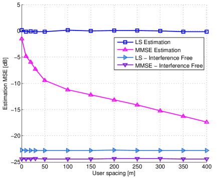
In Fig. 8, we assume the target user is located at the origin while an interfering user (they share the same pilot sequence) is moving over the horizontal axis at increasing distances from user 1. As we can observe, when the MMSE estimator (4) is used, the channel estimation error is a monotonous decreasing function of the distance between the desired user and the interference user. One may also notice the constant performance gap between LS and MMSE estimator in interference-free scenario, which indicates that covariance information is still helpful even in a highly distributed antenna system. As shown in the blue curve on the top, an LS estimator is unable to separate the desired channel and the interference channel. In contrast, an MMSE estimator has much better performance as its MSE is decreasing almost linearly with inter-user spacing, hence confirming our claims.
Refer to caption
Figure 8: Estimation performance vs. distance between two users, M=2000𝑀2000M=2000, r=15𝑟15r=15m, single-cell network.

We then examine the performance of four MRC beamformers in terms of uplink sum-rate in a single-cell setting (Fig. 9) and per-cell rate in a multi-cell setting (Fig. 10). The sum-rate is defined as follows:

sum-ratek=1Klog2(1+SINRk),sum-ratesuperscriptsubscript𝑘1𝐾subscriptlog21subscriptSINR𝑘\text{sum-rate}\triangleq{{\sum\limits_{k=1}^{K}{{\text{log}}_{2}(1+\text{SINR}_{k})}}}, (32)

where K𝐾K is the number of simultaneously served users, and SINRksubscriptSINR𝑘{\text{SINR}}_{k} is the uplink signal-to-noise-plus-interference ratio (SINR) of the k𝑘k-th user.

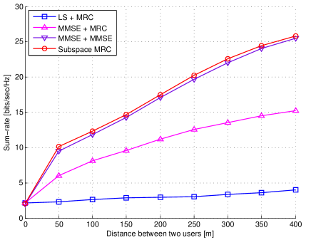
In Fig. 9, we show the performance of subspace-based MRC beamforming in a single-cell network where two users share the same pilot. The total number of distributed antennas is 500. In the figure “LS + MRC” denotes the sum-rate performance of MRC beamforming using the LS channel estimate, while the curve “MMSE + MRC” is the performance of MRC beamforming using the MMSE estimate (4). “MMSE + MMSE” denotes the performance curve of MMSE beamforming using MMSE channel estimate when channel covariances (including the interference covariances) are assumed known during both channel estimation and signal detection. The simulation shows the simple subspace-based method has a very good performance. Due to pilot contamination, the MRC beamformer using MMSE channel estimate is not as good as subspace-based method. The reason is that 𝐑1subscript𝐑1\mathbf{R}_{1} and 𝐑2subscript𝐑2\mathbf{R}_{2} generally have overlapping signal subspaces here. We may also notice that the subspace-based MRC beamformer has some slight performance gains over the MMSE beamformer.
Refer to caption
Figure 9: Uplink sum-rate vs. distance between 2 users, M=500𝑀500M=500, r=15𝑟15r=15m, cell-edge SNR 20dB, single-cell network.

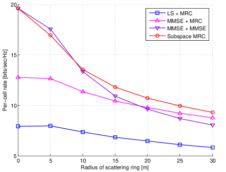
Fig. 10 depicts the uplink per-cell rate achieved by the above-mentioned MRC beamformers as a function of scattering radius r𝑟r. In the simulation we have 7 hexagonal cells with one center cell and 6 surrounding cells. Each cell has one user. All the users share the same pilot sequence. The per-cell rate is defined as the sum-rate (32) divided by the number of cells. As can be seen, the subspace-based beamforming shows performance gains over other traditional MRC methods especially when the radius of scattering ring is smaller. It also shows more robustness than MMSE beamformer when the radius of the scattering ring is larger.
Refer to caption
Figure 10: Uplink per-cell rate vs. r𝑟r, cell-edge SNR 20dB, 7-cell network, each cell has M=500𝑀500M=500 distributed antennas.

VI Conclusions

We investigate low-dimensional properties of covariance signal subspaces in general topologies of massive arrays. We extend previous results known in the uniform linear array case to the case of arrays with random placement, including the case of scattered antennas over a 2D dense network. A correlation model is derived which is exploited to gain insight on the interference rejection capability of low-complexity matched filter-based receivers in distributed antenna settings.

-A Proof of Proposition 2:

We first consider an N𝑁N-antenna ULA with aperture 𝒟𝒟\mathcal{D} and antenna spacing D=𝒟/(N1)𝐷𝒟𝑁1D=\mathcal{D}/(N-1). Define

𝜶~(x)~𝜶𝑥\displaystyle\tilde{\boldsymbol{\alpha}}(x) [0,ej2πDλx,,ej2πD(N1)λx]Tabsentsuperscript0superscript𝑒𝑗2𝜋𝐷𝜆𝑥superscript𝑒𝑗2𝜋𝐷𝑁1𝜆𝑥𝑇\displaystyle\triangleq\left[0,{{e^{-j2\pi\frac{D}{\lambda}x}}},\cdots,{{e^{-j2\pi\frac{D(N-1)}{\lambda}x}}}\right]^{T}
=[0,ej2π𝒟λ(N1)x,,ej2π𝒟(N1)λ(N1)x]T.absentsuperscript0superscript𝑒𝑗2𝜋𝒟𝜆𝑁1𝑥superscript𝑒𝑗2𝜋𝒟𝑁1𝜆𝑁1𝑥𝑇\displaystyle=\left[0,{{e^{-j2\pi\frac{\mathcal{D}}{\lambda(N-1)}x}}},\cdots,{{e^{-j2\pi\frac{\mathcal{D}(N-1)}{\lambda(N-1)}x}}}\right]^{T}.

Now we define 𝒜~span{𝜶~(x),x[b1,b2]}~𝒜span~𝜶𝑥𝑥subscript𝑏1subscript𝑏2\tilde{\mathcal{A}}\triangleq\operatorname{span}\{\tilde{\boldsymbol{\alpha}}{(x)},{x}\in[{b_{1}},{b_{2}}]\}. Recall from [10] the following result:

If 𝜷(x)[1ejπxejπ(N1)x]T𝜷(x)superscriptdelimited-[]1superscript𝑒𝑗𝜋𝑥superscript𝑒𝑗𝜋𝑁1𝑥missing-subexpressionmissing-subexpressionmissing-subexpressionmissing-subexpressionmissing-subexpressionmissing-subexpressionmissing-subexpressionmissing-subexpressionmissing-subexpressionmissing-subexpressionmissing-subexpressionmissing-subexpressionmissing-subexpressionmissing-subexpressionmissing-subexpressionmissing-subexpression𝑇{\boldsymbol{\beta}}{\text{(x)}}\triangleq{[\begin{array}[]{*{20}{c}}1&{{e^{-j\pi x}}}&\cdots&{{e^{-j\pi(N-1)x}}}\end{array}]^{T}}. Given b1,b2[1,1]subscript𝑏1subscript𝑏211{b_{1}},{b_{2}}\in[-1,1] and b1<b2subscript𝑏1subscript𝑏2{b_{1}}<{b_{2}}, define 𝒜span{𝜷(x),x[b1,b2]}𝒜span𝜷(x)xsubscript𝑏1subscript𝑏2\mathcal{A}\triangleq\operatorname{span}\{{\boldsymbol{\beta}}{\text{(x)}},{\text{x}}\in[{b_{1}},{b_{2}}]\}, when N𝑁N is large,

dim{𝒜}=(b2b1)N2+o((b2b1)N2).dimension𝒜subscript𝑏2subscript𝑏1𝑁2𝑜subscript𝑏2subscript𝑏1𝑁2\dim\{\mathcal{A}\}=\frac{({b_{2}}-{b_{1}})N}{2}+o(\frac{({b_{2}}-{b_{1}})N}{2}). (33)

The above conclusion can directly apply: when N𝑁N is large,

dim{𝒜~}dimension~𝒜\displaystyle\dim\{\tilde{\mathcal{A}}\} =N𝒟(N1)λ(b2b1)+o(N𝒟(N1)λ(b2b1))absent𝑁𝒟𝑁1𝜆subscript𝑏2subscript𝑏1𝑜𝑁𝒟𝑁1𝜆subscript𝑏2subscript𝑏1\displaystyle=\frac{N\mathcal{D}}{(N-1)\lambda}({b_{2}}-{b_{1}})+o\left(\frac{N\mathcal{D}}{(N-1)\lambda}({b_{2}}-{b_{1}})\right)
=DNλ(b2b1)+o(DNλ(b2b1))absent𝐷𝑁𝜆subscript𝑏2subscript𝑏1𝑜𝐷𝑁𝜆subscript𝑏2subscript𝑏1\displaystyle=\frac{{D}N}{\lambda}({b_{2}}-{b_{1}})+o\left(\frac{{D}N}{\lambda}({b_{2}}-{b_{1}})\right)
=MD¯λ(b2b1)+o(MD¯λ(b2b1))absent𝑀¯𝐷𝜆subscript𝑏2subscript𝑏1𝑜𝑀¯𝐷𝜆subscript𝑏2subscript𝑏1\displaystyle=\frac{M\overline{D}}{\lambda}({b_{2}}-{b_{1}})+o\left(\frac{M\overline{D}}{\lambda}({b_{2}}-{b_{1}})\right)
=MD¯λ(b2b1)+o(M).absent𝑀¯𝐷𝜆subscript𝑏2subscript𝑏1𝑜𝑀\displaystyle=\frac{M\overline{D}}{\lambda}({b_{2}}-{b_{1}})+o(M).

We can observe that dim{𝒜~}dimension~𝒜\dim\{\tilde{\mathcal{A}}\} has no dependency on N𝑁N. Imagine for any finite aperture 𝒟𝒟\mathcal{D}, we let N𝑁N\rightarrow\infty so that D0𝐷0D\rightarrow 0. In this case, all elements of 𝜶(x)𝜶𝑥{\boldsymbol{\alpha}}{(x)} can be seen as M𝑀M (finite) random samples in the vector 𝜶~(x)~𝜶𝑥\tilde{\boldsymbol{\alpha}}(x). Hence

dim{}dim{𝒜~}=MD¯λ(b2b1)+o(M).dimensiondimension~𝒜𝑀¯𝐷𝜆subscript𝑏2subscript𝑏1𝑜𝑀\dim\{\mathcal{B}\}\leq\dim\{\tilde{\mathcal{A}}\}=\frac{M\overline{D}}{\lambda}({b_{2}}-{b_{1}})+o(M).

Now consider the space 𝒞𝒞\mathcal{C}. We define 𝒞qspan{𝜶(x),x[bqmin,bqmax]}subscript𝒞𝑞span𝜶𝑥𝑥subscriptsuperscript𝑏min𝑞subscriptsuperscript𝑏max𝑞\mathcal{C}_{q}\triangleq\operatorname{span}\{{\boldsymbol{\alpha}}{(x)},{x}\in[{b^{\text{min}}_{q}},{b^{\text{max}}_{q}}]\}. An upper bound of its dimension can be obtained by considering the extreme case when all Q𝑄Q spaces are mutually orthogonal so that their dimensions can add up:

dim{𝒞}q=1Qdim{𝒞q}=q=1QMD¯λ(bqmaxbqmin)+o(M).dimension𝒞superscriptsubscript𝑞1𝑄dimensionsubscript𝒞𝑞superscriptsubscript𝑞1𝑄𝑀¯𝐷𝜆subscriptsuperscript𝑏max𝑞subscriptsuperscript𝑏min𝑞𝑜𝑀\dim\{\mathcal{C}\}\leq\sum_{q=1}^{Q}\dim\{{\mathcal{C}_{q}}\}=\sum_{q=1}^{Q}\frac{M\overline{D}}{\lambda}({b^{\text{max}}_{q}}-{b^{\text{min}}_{q}})+o(M).

Thus, Proposition 2 is proven.   

-B Proof of Theorem 1:

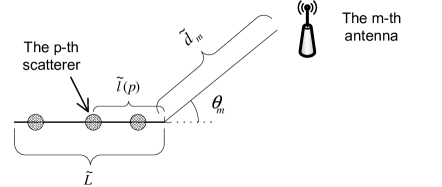
For ease of exposition we omit the user index k𝑘k. Imagine a special case when the scatterers are located in a line which has the length L~~𝐿\tilde{L}, as shown in Fig. 11. Assume the antennas are far away so that the scatterers are in the same planar wavefront region. We denote the right end of the scattering line as the reference point. The m𝑚m-th antenna is located d~msubscript~𝑑𝑚\tilde{d}_{m} meters away from the reference point, at the angle θmsubscript𝜃𝑚\theta_{m}. The p𝑝p-th scatter is l~(p)~𝑙𝑝\tilde{l}(p) meters away from the reference point. l~(p)~𝑙𝑝\tilde{l}(p) follows a uniform distribution, i.e., l~(p)𝒰(0,L~)similar-to~𝑙𝑝𝒰0~𝐿\tilde{l}(p)\sim\mathcal{U}(0,\tilde{L}). The phase shift between the scatterer p𝑝p and the reference point is 2πl~(p)cos(θm)/λ2𝜋~𝑙𝑝subscript𝜃𝑚𝜆2\pi\tilde{l}(p)\cos(\theta_{m})/\lambda, 1mM1𝑚𝑀1\leq m\leq M.

Refer to caption
Figure 11: Illustration of a line of scatterers.

Define a diagonal phase matrix

𝚵diag{ej2πd~1+rλ,,ej2πd~M+rλ}.𝚵diagsuperscript𝑒𝑗2𝜋subscript~𝑑1𝑟𝜆superscript𝑒𝑗2𝜋subscript~𝑑𝑀𝑟𝜆\mathbf{\Xi}\triangleq{\mathop{\rm diag}\nolimits}\{{{e^{-j2\pi\frac{\tilde{d}_{1}+r}{\lambda}},...,e^{-j2\pi\frac{\tilde{d}_{M}+r}{\lambda}}}}\}.

The p𝑝p-th scattering path vector channel is now given by:

𝐡p[ej2πdp1+rλej2πdpM+rλ]ejφp=ejφp𝚵[ej2πl~(p)cos(θ1)λej2πl~(p)cos(θM)λ]subscript𝐡𝑝delimited-[]superscript𝑒𝑗2𝜋subscript𝑑𝑝1𝑟𝜆missing-subexpressionmissing-subexpressionmissing-subexpressionmissing-subexpressionmissing-subexpressionmissing-subexpressionmissing-subexpressionmissing-subexpressionmissing-subexpressionmissing-subexpressionmissing-subexpressionmissing-subexpressionmissing-subexpressionmissing-subexpressionmissing-subexpressionmissing-subexpressionmissing-subexpressionmissing-subexpressionmissing-subexpressionmissing-subexpressionmissing-subexpressionmissing-subexpressionmissing-subexpressionmissing-subexpressionmissing-subexpressionmissing-subexpressionmissing-subexpressionmissing-subexpressionmissing-subexpressionmissing-subexpressionmissing-subexpressionmissing-subexpressionmissing-subexpressionmissing-subexpressionmissing-subexpressionmissing-subexpressionmissing-subexpressionmissing-subexpressionsuperscript𝑒𝑗2𝜋subscript𝑑𝑝𝑀𝑟𝜆missing-subexpressionmissing-subexpressionmissing-subexpressionmissing-subexpressionmissing-subexpressionmissing-subexpressionmissing-subexpressionmissing-subexpressionmissing-subexpressionmissing-subexpressionmissing-subexpressionmissing-subexpressionmissing-subexpressionmissing-subexpressionmissing-subexpressionmissing-subexpressionmissing-subexpressionmissing-subexpressionmissing-subexpressionsuperscript𝑒𝑗subscript𝜑𝑝superscript𝑒𝑗subscript𝜑𝑝𝚵delimited-[]superscript𝑒𝑗2𝜋~𝑙𝑝subscript𝜃1𝜆missing-subexpressionmissing-subexpressionmissing-subexpressionmissing-subexpressionmissing-subexpressionmissing-subexpressionmissing-subexpressionmissing-subexpressionmissing-subexpressionmissing-subexpressionmissing-subexpressionmissing-subexpressionmissing-subexpressionmissing-subexpressionmissing-subexpressionmissing-subexpressionmissing-subexpressionmissing-subexpressionmissing-subexpressionmissing-subexpressionmissing-subexpressionmissing-subexpressionmissing-subexpressionmissing-subexpressionmissing-subexpressionmissing-subexpressionmissing-subexpressionmissing-subexpressionmissing-subexpressionmissing-subexpressionmissing-subexpressionmissing-subexpressionmissing-subexpressionmissing-subexpressionmissing-subexpressionmissing-subexpressionmissing-subexpressionmissing-subexpressionsuperscript𝑒𝑗2𝜋~𝑙𝑝subscript𝜃𝑀𝜆missing-subexpressionmissing-subexpressionmissing-subexpressionmissing-subexpressionmissing-subexpressionmissing-subexpressionmissing-subexpressionmissing-subexpressionmissing-subexpressionmissing-subexpressionmissing-subexpressionmissing-subexpressionmissing-subexpressionmissing-subexpressionmissing-subexpressionmissing-subexpressionmissing-subexpressionmissing-subexpressionmissing-subexpression{\mathbf{h}_{p}}\triangleq\left[{\begin{array}[]{*{20}{c}}{e^{-j2\pi\frac{d_{p1}+r}{\lambda}}}\\ \vdots\\ {e^{-j2\pi\frac{d_{pM}+r}{\lambda}}}\end{array}}\right]e^{j\varphi_{p}}=e^{j\varphi_{p}}\mathbf{\Xi}\left[{\begin{array}[]{*{20}{c}}{e^{-j2\pi\frac{\tilde{l}(p)\cos(\theta_{1})}{\lambda}}}\\ \vdots\\ {e^{-j2\pi\frac{\tilde{l}(p)\cos(\theta_{M})}{\lambda}}}\end{array}}\right]

If we define 𝐡~p[ej2πl~(p)cos(θ1)λ,,ej2πl~(p)cos(θM)λ]Tsubscript~𝐡𝑝superscriptsuperscript𝑒𝑗2𝜋~𝑙𝑝subscript𝜃1𝜆superscript𝑒𝑗2𝜋~𝑙𝑝subscript𝜃𝑀𝜆𝑇\tilde{\mathbf{h}}_{p}\triangleq[{e^{-j2\pi\frac{\tilde{l}(p)\cos(\theta_{1})}{\lambda}}},\cdots,{e^{-j2\pi\frac{\tilde{l}(p)\cos(\theta_{M})}{\lambda}}}]^{T}, we may see that 𝐡~psubscript~𝐡𝑝\tilde{\mathbf{h}}_{p} and 𝐡psubscript𝐡𝑝\mathbf{h}_{p} are unitarily equivalent, since ejφp𝚵superscript𝑒𝑗subscript𝜑𝑝𝚵e^{j\varphi_{p}}\mathbf{\Xi} forms a unitary matrix. If we vary l~(p)~𝑙𝑝\tilde{l}(p), we can obtain two linear spaces spanned by 𝐡psubscript𝐡𝑝\mathbf{h}_{p} and/or 𝐡~psubscript~𝐡𝑝\tilde{\mathbf{h}}_{p}. The dimensions of the two spaces are equal. Therefore in the following we will find the dimension spanned by 𝐡~psubscript~𝐡𝑝\tilde{\mathbf{h}}_{p} instead of 𝐡psubscript𝐡𝑝\mathbf{h}_{p}. Assume N𝑁N is a large integer, we define xn1+2(n1)N,n=1,,Nformulae-sequencesubscript𝑥𝑛12𝑛1𝑁𝑛1𝑁x_{n}\triangleq-1+\frac{2(n-1)}{N},n=1,...,N, the set 𝒳{xn}𝒳subscript𝑥𝑛\mathcal{X}\triangleq\{x_{n}\}, as well as the vector

𝝁p[ej2πl~(p)x1λej2πl~(p)x2λej2πl~(p)xNλ]=ej2πl~(p)[ej2πl~(p)(0)λej2πl~(p)(2N)λej2πl~(p)(2(N1)N)λ].subscript𝝁𝑝delimited-[]superscript𝑒𝑗2𝜋~𝑙𝑝subscript𝑥1𝜆missing-subexpressionmissing-subexpressionmissing-subexpressionmissing-subexpressionmissing-subexpressionmissing-subexpressionmissing-subexpressionmissing-subexpressionmissing-subexpressionmissing-subexpressionmissing-subexpressionmissing-subexpressionmissing-subexpressionmissing-subexpressionmissing-subexpressionmissing-subexpressionmissing-subexpressionmissing-subexpressionmissing-subexpressionsuperscript𝑒𝑗2𝜋~𝑙𝑝subscript𝑥2𝜆missing-subexpressionmissing-subexpressionmissing-subexpressionmissing-subexpressionmissing-subexpressionmissing-subexpressionmissing-subexpressionmissing-subexpressionmissing-subexpressionmissing-subexpressionmissing-subexpressionmissing-subexpressionmissing-subexpressionmissing-subexpressionmissing-subexpressionmissing-subexpressionmissing-subexpressionmissing-subexpressionmissing-subexpressionmissing-subexpressionmissing-subexpressionmissing-subexpressionmissing-subexpressionmissing-subexpressionmissing-subexpressionmissing-subexpressionmissing-subexpressionmissing-subexpressionmissing-subexpressionmissing-subexpressionmissing-subexpressionmissing-subexpressionmissing-subexpressionmissing-subexpressionmissing-subexpressionmissing-subexpressionmissing-subexpressionmissing-subexpressionsuperscript𝑒𝑗2𝜋~𝑙𝑝subscript𝑥𝑁𝜆missing-subexpressionmissing-subexpressionmissing-subexpressionmissing-subexpressionmissing-subexpressionmissing-subexpressionmissing-subexpressionmissing-subexpressionmissing-subexpressionmissing-subexpressionmissing-subexpressionmissing-subexpressionmissing-subexpressionmissing-subexpressionmissing-subexpressionmissing-subexpressionmissing-subexpressionmissing-subexpressionmissing-subexpressionsuperscript𝑒𝑗2𝜋~𝑙𝑝delimited-[]superscript𝑒𝑗2𝜋~𝑙𝑝0𝜆missing-subexpressionmissing-subexpressionmissing-subexpressionmissing-subexpressionmissing-subexpressionmissing-subexpressionmissing-subexpressionmissing-subexpressionmissing-subexpressionmissing-subexpressionmissing-subexpressionmissing-subexpressionmissing-subexpressionmissing-subexpressionmissing-subexpressionmissing-subexpressionmissing-subexpressionmissing-subexpressionmissing-subexpressionsuperscript𝑒𝑗2𝜋~𝑙𝑝2𝑁𝜆missing-subexpressionmissing-subexpressionmissing-subexpressionmissing-subexpressionmissing-subexpressionmissing-subexpressionmissing-subexpressionmissing-subexpressionmissing-subexpressionmissing-subexpressionmissing-subexpressionmissing-subexpressionmissing-subexpressionmissing-subexpressionmissing-subexpressionmissing-subexpressionmissing-subexpressionmissing-subexpressionmissing-subexpressionmissing-subexpressionmissing-subexpressionmissing-subexpressionmissing-subexpressionmissing-subexpressionmissing-subexpressionmissing-subexpressionmissing-subexpressionmissing-subexpressionmissing-subexpressionmissing-subexpressionmissing-subexpressionmissing-subexpressionmissing-subexpressionmissing-subexpressionmissing-subexpressionmissing-subexpressionmissing-subexpressionmissing-subexpressionsuperscript𝑒𝑗2𝜋~𝑙𝑝2𝑁1𝑁𝜆missing-subexpressionmissing-subexpressionmissing-subexpressionmissing-subexpressionmissing-subexpressionmissing-subexpressionmissing-subexpressionmissing-subexpressionmissing-subexpressionmissing-subexpressionmissing-subexpressionmissing-subexpressionmissing-subexpressionmissing-subexpressionmissing-subexpressionmissing-subexpressionmissing-subexpressionmissing-subexpressionmissing-subexpression\boldsymbol{\mu}_{p}\triangleq\left[{\begin{array}[]{*{20}{c}}{e^{-j2\pi\frac{\tilde{l}(p)x_{1}}{\lambda}}}\\ {e^{-j2\pi\frac{\tilde{l}(p)x_{2}}{\lambda}}}\\ \vdots\\ {e^{-j2\pi\frac{\tilde{l}(p)x_{N}}{\lambda}}}\end{array}}\right]=e^{j2\pi\tilde{l}(p)}\left[{\begin{array}[]{*{20}{c}}{e^{-j2\pi\frac{\tilde{l}(p)(0)}{\lambda}}}\\ {e^{-j2\pi\frac{\tilde{l}(p)(\frac{2}{N})}{\lambda}}}\\ \vdots\\ {e^{-j2\pi\frac{\tilde{l}(p)(\frac{2(N-1)}{N})}{\lambda}}}\end{array}}\right].

Since l~(p)𝒰(0,L~)similar-to~𝑙𝑝𝒰0~𝐿\tilde{l}(p)\sim\mathcal{U}(0,\tilde{L}), we reuse the result shown in (33):

dim{span{𝝁p,l~(p)[0,L~]}}dimensionspansubscript𝝁𝑝~𝑙𝑝0~𝐿\displaystyle\dim\{\operatorname{span}\{\boldsymbol{\mu}_{p},\tilde{l}(p)\in[0,\tilde{L}]\}\}
=4L~NλN2+o(4L~NλN2)absent4~𝐿𝑁𝜆𝑁2𝑜4~𝐿𝑁𝜆𝑁2\displaystyle=\frac{4\tilde{L}}{N\lambda}\frac{N}{2}+o\left(\frac{4\tilde{L}}{N\lambda}\frac{N}{2}\right)
=2L~λ+o(L~).absent2~𝐿𝜆𝑜~𝐿\displaystyle=\frac{2\tilde{L}}{\lambda}+o(\tilde{L}).

Note that the above result holds when N𝑁N is arbitrarily large. We again observe that when N𝑁N\rightarrow\infty, any cos(θm)subscript𝜃𝑚\cos(\theta_{m}) will fall into the set 𝒳𝒳\mathcal{X}, which indicates

dim{span{𝐡~p,l~(p)[0,L~]}}2L~λ+o(L~).dimensionspansubscript~𝐡𝑝~𝑙𝑝0~𝐿2~𝐿𝜆𝑜~𝐿\dim\{\operatorname{span}\{\tilde{\mathbf{h}}_{p},\tilde{l}(p)\in[0,\tilde{L}]\}\}\leq\frac{2\tilde{L}}{\lambda}+o(\tilde{L}). (34)

Recall that the covariance matrix 𝐑=𝔼{1Pp=1Pq=1P𝐡p𝐡qH}𝐑𝔼1𝑃superscriptsubscript𝑝1𝑃superscriptsubscript𝑞1𝑃subscript𝐡𝑝superscriptsubscript𝐡𝑞𝐻\mathbf{R}=\mathbb{E}\{\frac{1}{{P}}\sum\limits_{p=1}^{P}\sum\limits_{q=1}^{P}{{{\mathbf{h}}_{p}}}{{{\mathbf{h}}_{q}^{H}}}\}. Because of the random and independent phases φpsubscript𝜑𝑝\varphi_{p} and φqsubscript𝜑𝑞\varphi_{q},

pq,𝔼{𝐡p𝐡qH}=𝟎.formulae-sequencefor-all𝑝𝑞𝔼subscript𝐡𝑝superscriptsubscript𝐡𝑞𝐻0\forall p\neq q,\mathbb{E}\{{\mathbf{h}}_{p}{{\mathbf{h}}_{q}^{H}}\}=\mathbf{0}.
𝐑=𝔼{1Pp=1P𝐡p𝐡pH}=𝔼{𝐡p𝐡pH}.𝐑𝔼1𝑃superscriptsubscript𝑝1𝑃subscript𝐡𝑝superscriptsubscript𝐡𝑝𝐻𝔼subscript𝐡𝑝superscriptsubscript𝐡𝑝𝐻\mathbf{R}=\mathbb{E}\{\frac{1}{{P}}\sum\limits_{p=1}^{P}{{{\mathbf{h}}_{p}}}{{{\mathbf{h}}_{p}^{H}}}\}=\mathbb{E}\{{\mathbf{h}}_{p}{{\mathbf{h}_{p}^{H}}}\}.

We can see that the number of scatterers has no impact on the rank of channel covariance matrix. Hence according to (34), the rank of 𝐑𝐑\mathbf{R} is upper bounded by

rank(𝐑)2L~λ+o(L~).rank𝐑2~𝐿𝜆𝑜~𝐿\text{rank}(\mathbf{R})\leq\frac{2\tilde{L}}{\lambda}+o(\tilde{L}).

Returning to the one-ring model, we can interpret the ring as the sum of lines, with the total length 2πr2𝜋𝑟2\pi r. An extreme case is when all of the channels corresponding to different pieces of the ring span orthogonal spaces, i.e., the rank of the covariance matrix is the sum of the spatial dimensions corresponding to every pieces of the ring. This is the case when the covariance rank is maximized. Therefore the rank is upper bounded by:

rank(𝐑)4πrλ+o(r).rank𝐑4𝜋𝑟𝜆𝑜𝑟\text{rank}(\mathbf{R})\leq\frac{4\pi r}{\lambda}+o(r).

Thus Theorem 1 is proven.   

-C Proof of Proposition 5

Proof: We split up the disk centered in the midpoint between the two scatterers into N𝑁N (a large number) equal-sized sectors like dividing up a cake. The BS antennas all fall into one of these sectors. We have

|𝐡2qH𝐡1p|superscriptsubscript𝐡2𝑞𝐻subscript𝐡1𝑝\displaystyle\left|{\mathbf{h}}_{2q}^{H}{{\mathbf{h}}_{1p}}\right| =limN|n=1Nm=1Mn(h2qnmh1pnm)|absentsubscript𝑁superscriptsubscript𝑛1𝑁superscriptsubscript𝑚1subscript𝑀𝑛superscriptsubscript2𝑞𝑛𝑚subscript1𝑝𝑛𝑚\displaystyle=\mathop{\lim}\limits_{N\to\infty}\left|\sum\limits_{n=1}^{N}{\sum\limits_{m=1}^{{M_{n}}}{\left({h_{2qnm}^{*}{h_{1pnm}}}\right)}}\right|
=limN|n=1Nm=1Mn(β2qnmβ1pnmej2πd2qnmd1pnmλ)|,absentsubscript𝑁superscriptsubscript𝑛1𝑁superscriptsubscript𝑚1subscript𝑀𝑛subscript𝛽2𝑞𝑛𝑚subscript𝛽1𝑝𝑛𝑚superscript𝑒𝑗2𝜋subscript𝑑2𝑞𝑛𝑚subscript𝑑1𝑝𝑛𝑚𝜆\displaystyle=\mathop{\lim}\limits_{N\to\infty}\left|\sum\limits_{n=1}^{N}{\sum\limits_{m=1}^{{M_{n}}}{\left({\sqrt{{\beta_{2qnm}}{\beta_{1pnm}}}{e^{j2\pi\frac{{{d_{2qnm}}-{d_{1pnm}}}}{\lambda}}}}\right)}}\right|,

where Mnsubscript𝑀𝑛M_{n} (could be zero) is the total number of antennas located in the n𝑛n-th sector, h2qnmsubscript2𝑞𝑛𝑚h_{2qnm} and h1pnmsubscript1𝑝𝑛𝑚h_{1pnm} are the channel coefficient between the m𝑚m-th antenna located in the n𝑛n-th sector and the two scatterers. If N𝑁N is large, the angle contained by the two sides of a sector is small. Therefore BS antennas located in the same sector share the same difference of distances between the two scatterers, i.e., d2qnmd1pnmsubscript𝑑2𝑞𝑛𝑚subscript𝑑1𝑝𝑛𝑚{d_{2qnm}}-{d_{1pnm}} only depends on the sector index n𝑛n. Based on the fact that Dpqsubscript𝐷𝑝𝑞D_{pq} is small, we assume β2qnmβ1pnmsubscript𝛽2𝑞𝑛𝑚subscript𝛽1𝑝𝑛𝑚{\beta_{2qnm}}\approx{\beta_{1pnm}} and d2qnmd1pnm=Dpqcos(αn)subscript𝑑2𝑞𝑛𝑚subscript𝑑1𝑝𝑛𝑚subscript𝐷𝑝𝑞subscript𝛼𝑛{d_{2qnm}}-{d_{1pnm}}=D_{pq}\cos(\alpha_{n}), where αn2πnNsubscript𝛼𝑛2𝜋𝑛𝑁\alpha_{n}\triangleq\frac{2\pi n}{N} is the AOA from the BS antennas in the n𝑛n-th sector.

|𝐡2qH𝐡1p|superscriptsubscript𝐡2𝑞𝐻subscript𝐡1𝑝\displaystyle|{\mathbf{h}}_{2q}^{H}{{\mathbf{h}}_{1p}}| =limN|n=1N(ej2πDpqcos(αn)λm=1Mnβ2qnmβ1pnm)|absentsubscript𝑁superscriptsubscript𝑛1𝑁superscript𝑒𝑗2𝜋subscript𝐷𝑝𝑞subscript𝛼𝑛𝜆superscriptsubscript𝑚1subscript𝑀𝑛subscript𝛽2𝑞𝑛𝑚subscript𝛽1𝑝𝑛𝑚\displaystyle=\mathop{\lim}\limits_{N\to\infty}\left|\sum\limits_{n=1}^{N}{\left({{e^{j2\pi\frac{{D_{pq}\cos({\alpha_{n}})}}{\lambda}}}\sum\limits_{m=1}^{{M_{n}}}{\sqrt{{{\beta_{2qnm}}{\beta_{1pnm}}}}}}\right)}\right|
limN|n=1N(ej2πDpqcos(αn)λm=1Mnβ1pnm)|,absentsubscript𝑁superscriptsubscript𝑛1𝑁superscript𝑒𝑗2𝜋subscript𝐷𝑝𝑞subscript𝛼𝑛𝜆superscriptsubscript𝑚1subscript𝑀𝑛subscript𝛽1𝑝𝑛𝑚\displaystyle\approx\mathop{\lim}\limits_{N\to\infty}\left|\sum\limits_{n=1}^{N}{\left({{e^{j2\pi\frac{{D_{pq}\cos({\alpha_{n}})}}{\lambda}}}\sum\limits_{m=1}^{{M_{n}}}{{\beta_{1pnm}}}}\right)}\right|,
|𝐡1p||𝐡2q||𝐡1p|2=limNn=1Nm=1Mnβ1pnm.subscript𝐡1𝑝subscript𝐡2𝑞superscriptsubscript𝐡1𝑝2subscript𝑁superscriptsubscript𝑛1𝑁superscriptsubscript𝑚1subscript𝑀𝑛subscript𝛽1𝑝𝑛𝑚\left|{{{\mathbf{h}}_{1p}}}\right|\left|{{{\mathbf{h}}_{2q}}}\right|\approx{\left|{{{\mathbf{h}}_{1p}}}\right|^{2}}=\mathop{\lim}\limits_{N\to\infty}\sum\limits_{n=1}^{N}{\sum\limits_{m=1}^{{M_{n}}}{\beta_{1pnm}}}.

Due to the symmetry of the network, when M𝑀M\rightarrow\infty, the radio waves can arrive from any direction with equal probability. Thus m=1Mnβ1pnmsuperscriptsubscript𝑚1subscript𝑀𝑛subscript𝛽1𝑝𝑛𝑚\sum\nolimits_{m=1}^{{M_{n}}}{\beta_{1pnm}} is independent of sector index n𝑛n.

limM|𝐡2qH𝐡1p||𝐡1p||𝐡2q|subscript𝑀superscriptsubscript𝐡2𝑞𝐻subscript𝐡1𝑝subscript𝐡1𝑝subscript𝐡2𝑞\displaystyle\mathop{\lim}\limits_{M\to\infty}\frac{|{\mathbf{h}}_{2q}^{H}{{\mathbf{h}}_{1p}}|}{{\left|{{{\mathbf{h}}_{1p}}}\right|\left|{{{\mathbf{h}}_{2q}}}\right|}} limN|1Nn=1Nej2πDpqcos(αn)λ|absentsubscript𝑁1𝑁superscriptsubscript𝑛1𝑁superscript𝑒𝑗2𝜋subscript𝐷𝑝𝑞subscript𝛼𝑛𝜆\displaystyle\approx\mathop{\lim}\limits_{N\to\infty}\left|\frac{1}{N}\sum\limits_{n=1}^{N}{{e^{j2\pi\frac{{{D_{pq}}\cos({\alpha_{n}})}}{\lambda}}}}\right|
=12π|02πej2πDpqcos(α)λ𝑑α|absent12𝜋superscriptsubscript02𝜋superscript𝑒𝑗2𝜋subscript𝐷𝑝𝑞𝛼𝜆differential-d𝛼\displaystyle=\frac{1}{{2\pi}}\left|\int_{0}^{2\pi}{{e^{j2\pi\frac{{D_{pq}\cos(\alpha)}}{\lambda}}}}d\alpha\right|
=|J0(2πDpqλ)|,absentsubscript𝐽02𝜋subscript𝐷𝑝𝑞𝜆\displaystyle=\left|{J_{0}}(\frac{{2\pi D_{pq}}}{\lambda})\right|,

and Proposition 5 is proven.   

References

  • [1] T. L. Marzetta, “Noncooperative cellular wireless with unlimited numbers of base station antennas,” IEEE Trans. Wireless Commun, vol. 9, no. 11, pp. 3590–3600, Nov. 2010.
  • [2] F. Rusek, D. Persson, B. K. Lau, E. G. Larsson, T. L. Marzetta, O. Edfors, and F. Tufvesson, “Scaling up MIMO: Opportunities and challenges with very large arrays,” IEEE Signal Process. Mag., vol. 30, no. 1, pp. 40–60, 2013.
  • [3] J. Hoydis, S. ten Brink, and M. Debbah, “Massive MIMO in the UL/DL of cellular networks: How many antennas do we need?” IEEE J. Sel. Areas Commun., vol. 31, no. 2, pp. 160–171, 2013.
  • [4] E. G. Larsson, F. Tufvesson, O. Edfors, and T. L. Marzetta, “Massive MIMO for next generation wireless systems,” vol. 52, no. 2, pp. 186–195, Feb. 2014.
  • [5] D. Gesbert, S. Hanly, H. Huang, S. Shamai Shitz, O. Simeone, and W. Yu, “Multi-cell MIMO cooperative networks: A new look at interference,” IEEE J. Sel. Areas Commun., vol. 28, no. 9, pp. 1380–1408, Dec. 2010.
  • [6] A. Lozano, R. Heath, and J. Andrews, “Fundamental limits of cooperation,” IEEE Trans. Inf. Theory, vol. 59, no. 9, pp. 5213–5226, 2013.
  • [7] J. Jose, A. Ashikhmin, T. L. Marzetta, and S. Vishwanath, “Pilot contamination and precoding in multi-cell TDD systems,” IEEE Trans. Wireless Commun., vol. 10, no. 8, pp. 2640–2651, Aug. 2011.
  • [8] H. Q. Ngo, T. L. Marzetta, and E. G. Larsson, “Analysis of the pilot contamination effect in very large multicell multiuser MIMO systems for physical channel models,” in Proc. IEEE International Conference on Acoustics, Speech and Signal Processing (ICASSP 11), Prague, Czech Republic, May 2011, pp. 3464–3467.
  • [9] E. Björnson, J. Hoydis, M. Kountouris, and M. Debbah, “Massive MIMO systems with non-ideal hardware: energy efficiency, estimation, and capacity limits,” Submitted to IEEE Trans. Inf. Theory, 2013. [Online]. Available: http://arxiv.org/abs/1307.2584
  • [10] H. Yin, D. Gesbert, M. Filippou, and Y. Liu, “A coordinated approach to channel estimation in large-scale multiple-antenna systems,” IEEE J. Sel. Areas Commun., vol. 31, no. 2, pp. 264–273, Feb. 2013.
  • [11] R. R. Müller, L. Cottatellucci, and M. Vehkaperä, “Blind pilot decontamination,” Submitted to IEEE J. Sel. Topics Signal Process, 2013. [Online]. Available: http://arxiv.org/abs/1309.6806
  • [12] H. Ngo, E. Larsson, and T. Marzetta, “The multicell multiuser MIMO uplink with very large antenna arrays and a finite-dimensional channel,” IEEE Trans. Commun., pp. 2350–2361, 2013.
  • [13] A. Adhikary, J. Nam, J.-Y. Ahn, and G. Caire, “Joint spatial division and multiplexing – the large-scale array regime,” IEEE Trans. Inf. Theory, vol. 59, no. 10, pp. 6441–6463, Oct 2013.
  • [14] W. C. Jakes, Mobile microwave communication.   Wiley, 1974.
  • [15] D. shan Shiu, G. Foschini, M. Gans, and J. Kahn, “Fading correlation and its effect on the capacity of multielement antenna systems,” IEEE Trans. Commun., vol. 48, no. 3, pp. 502–513, Mar. 2000.
  • [16] R. A. Kennedy, P. Sadeghi, T. D. Abhayapala, and H. M. Jones, “Intrinsic limits of dimensionality and richness in random multipath fields,” IEEE Trans Signal Process., vol. 55, no. 6, pp. 2542–2556, 2007.
  • [17] A. F. Molisch, Wireless communications.   Wiley, 2010.
  • [18] E. Bjornson and B. Ottersten, “A framework for training-based estimation in arbitrarily correlated Rician MIMO channels with Rician disturbance,” IEEE Trans. Signal Process., vol. 58, no. 3, pp. 1807–1820, Mar. 2010.
  • [19] J. A. Tsai, R. M. Buehrer, and B. D. Woerner, “The impact of AOA energy distribution on the spatial fading correlation of linear antenna array,” in Proc. IEEE Vehicular Technology Conference, (VTC 02), vol. 2, May 2002, pp. 933–937.
  • [20] S. M. Kay, Fundamentals of Statistical Signal Processing: Estimation Theory.   Englewood Cliffs, NJ: Prentice Hall, 1993.
  • [21] J. A. Fill and D. E. Fishkind, “The Moore–Penrose generalized inverse for sums of matrices,” SIAM Journal on Matrix Analysis and Applications, vol. 21, no. 2, pp. 629–635, 2000.
  • [22] M. A. Rakha, “On the Moore–Penrose generalized inverse matrix,” Applied Mathematics and Computation, vol. 158, no. 1, pp. 185–200, 2004.
  • [23] I. Krasikov, “Uniform bounds for bessel functions,” Journal of Applied Analysis, vol. 12, no. 1, pp. 83–91, 2006.
  • [24] R. H. Clarke, “A statistical theory of mobile-radio reception,” Bell System Technical Journal, vol. 47, no. 6, pp. 957–1000, 1968.
Haifan Yin received the B.Sc. degree in Electrical and Electronic Engineering and the M.Sc. degree in Electronics and Information Engineering from Huazhong University of Science and Technology, Wuhan, China, in 2009 and 2012 respectively. From 2009 to 2011, he had been with Wuhan National Laboratory for Optoelectronics, China, working on the implementation of TD-LTE systems as an R&D engineer. In September 2012, he joined the Mobile Communications Department at EURECOM, France, where he is now a Ph.D. student. His current research interests include channel estimation, multi-cell cooperative networks, and large-scale antenna systems.
David Gesbert (IEEE Fellow) is Professor and Head of the Mobile Communications Department, EURECOM, France. He obtained the Ph.D degree from Ecole Nationale Superieure des Telecommunications, France, in 1997. From 1997 to 1999 he has been with the Information Systems Laboratory, Stanford University. In 1999, he was a founding engineer of Iospan Wireless Inc, San Jose, Ca.,a startup company pioneering MIMO-OFDM (now Intel). Between 2001 and 2003 he has been with the Department of Informatics, University of Oslo as an adjunct professor. D. Gesbert has published about 200 papers and several patents all in the area of signal processing, communications, and wireless networks. D. Gesbert was a co-editor of several special issues on wireless networks and communications theory, for JSAC (2003, 2007, 2009), EURASIP Journal on Applied Signal Processing (2004, 2007), Wireless Communications Magazine (2006). He served on the IEEE Signal Processing for Communications Technical Committee, 2003-2008. He authored or co-authored papers winning the 2004 IEEE Best Tutorial Paper Award (Communications Society) for a 2003 JSAC paper on MIMO systems, 2005 Best Paper (Young Author) Award for Signal Proc. Society journals, and the Best Paper Award for the 2004 ACM MSWiM workshop. He co-authored the book “Space time wireless communications: From parameter estimation to MIMO systems”, Cambridge Press, 2006.
Laura Cottatellucci is currently assistant professor at the Dept. of Mobile Communications in Eurecom. She obtained the PhD from Technical University of Vienna, Austria (2006). Specialized in networking at Guglielmo Reiss Romoli School (1996, Italy), she worked in Telecom Italia (1995-2000) as responsible of industrial projects. From April 2000 to September 2005 she worked as senior research in ftw Austria on CDMA and MIMO systems. From October to December 2005 she was research fellow on ad-hoc networks in INRIA (Sophia Antipolis, France) and guest researcher in Eurecom. In 2006 she was appointed research fellow at the University of South Australia, Australia to work on information theory for networks with uncertain topology. Cottatellucci is co-editor of a special issue on cooperative communications for EURASIP Journal on Wireless Communications and Networking and co-chair of RAWNET/WCN3 2009 in WiOpt. Her research topics of interest are large system analysis of wireless and complex networks based on random matrix theory and game theory.