Bound state techniques to solve the multiparticle scattering problem

Abstract

Solution of the scattering problem turns to be very difficult task both from the formal as well as from the computational point of view. If the last two decades have witnessed decisive progress in ab initio bound state calculations, rigorous solution of the scattering problem remains limited to A$\leq$4 case. Therefore there is a rising interest to apply bound-state-like methods to handle non-relativistic scattering problems. In this article the latest theoretical developments in this field are reviewed. Five fully rigorous methods will be discussed, which address the problem of nuclear collisions in full extent (including the break-up problem) at the same time avoiding treatment of the complicate boundary conditions or integral kernel singularities. These new developments allows to use modern bound-state techniques to advance significantly rigorous solution of the scattering problem.

1 Introduction

Numerically exact solutions of the multi-particle scattering problem have been, in the last 30 years, dominated by calculations of the three-nucleon system [1, 2, 3] where the early development of formally exact theories [4, 5] led to calculations that soon became numerically converged for a number of realistic interaction models some of which based on meson field theory [6, 7, 8], others derived from QCD using effective field theory [9, 10, 11].

The most ambitious solutions of the three-particle scattering problem only became possible by the emergence of larger and faster computers in the late eighties of the last century [1, 12, 13, 14]. Calculation methods based on the solution of momentum space integral equations could be achieved, both below and above three-particle breakup, using real axis integration together with spline interpolation and subtraction methods to handle the singularities that exist along the momentum axis for real energy [1]. The sole draw back that subsided for many years in momentum space calculations was the ability to include the long range Coulomb interaction between charged particles that was finally overcome in 2005 [15, 16] using a very simple but efficient screening procedure of the Coulomb interaction followed by the renormalization of the scattering amplitudes, that leads to a fast convergence of the calculated observables in terms of screening radius.

Unlike momentum space calculations, coordinate space methods based on formally exact theories were able to include the Coulomb interaction since the very early developments by using appropriate boundary conditions, leading to the interpretation of the existing data for charge particle reactions which are in general more abundant, easy to measure and more accurate. This is the case for proton-deuteron elastic scattering where numerically converged solutions have been around for many years using Kohn variational principle together with the hyperspherical harmonics expansion method [2] or Faddeev equations [17]. A number of benchmark calculations [14, 18, 19, 20] have been performed over the years and demonstrate that momentum space and coordinate space methods provide equally accurate solutions for neutron-deuteron (n-d) and proton-deuteron (p-d) elastic scattering, both below and above three-particle breakup threshold. Nevertheless, unlike momentum space calculations, the Achilles heel of coordinate space calculations has been so far the calculation of three-particle breakup observables due to numerical difficulties associated with matching, at a chosen boundary where the interactions are considered negligible, a complicated analytic asymptotic wave function to the numerical solution of the Schrödinger equation calculated from inside out. Given the oscillatory behavior of continuum wave functions for positive real energy, this matching in six-dimension space is the source of numerical inaccuracies and instabilities in the calculated observables. Recently three different methods which allow to solve the break-up problem without an explicit use of the asymptotic form of system wave function, and thus apply bound-state-like basis, have emerged with growing success.

The very first idea of using bound state solutions to solve many-body scattering problems is already present in Wigners R-matrix theory [21, 22, 23]. In this approach the scattering observables were obtained from configuration space solutions in the interaction region, which were expanded in squared integrable basis functions and thus without imposing the appropriate boundary conditions. However, at least in the nuclear physics case, this method was mostly used to solve scattering problems with only binary (elastic and rearrangement) channels open. Furthermore this method requires full diagonalization of the Hamiltonian representing matrix; thus, the resulting linear algebra problem must be of limited size to remain treatable numerically. Therefore the R-matrix method has been mostly applied [25, 24, 26] to handle simplified model problems (models with primitive interactions or including approximate dynamics) rather than providing exact solutions for few-body problems.

The first successful application of bound state methods to the calculation of observables, both below and above breakup threshold has been developed in Trento [27] to treat processes that are driven by an external source such as a photon or an electron. The photo disintegration of ${}^{3}\mathrm{He}$ [28, 29], ${}^{4}\mathrm{He}$ [30] and other light nuclei [31, 32, 33] or the electron disintegration $(e,ep)$ of bound light clusters [34] have been calculated using the Lorentz Integral Transform (LIT) which is the natural extension of an original idea to calculate reaction cross sections with the help of integral transforms. This method concentrates directly on matrix elements instead of trying to calculate wave functions and therefore avoids solving the Schrödinger equation in the continuum. Using clever integral transforms together with a chosen Lorentz kernel, the LIT method can reduce a continuum problem to a much less problematic bound-state-like problem. Nevertheless, since the LIT method has not yet been used successfully to calculate hadronic reactions, the solution of coordinate space Faddeev-like equations [4] above breakup has to rely on other methods, like complex scaling where the coordinates r are multiplied by a complex unit phase leading to their rotation by an angle $\theta$. With an appropriate choice of $\theta$ that depends on how the interaction behaves at large distances one is able to convert the solution of a continuum equation into a bound state like one. This method has been applied to handle very diverse problems [35, 36, 37, 38, 39, 40, 41, 42], can cope with realistic interactions [43, 44], and the results compare well with other calculation methods.

If the three-particle scattering problem is complicated, the four-particle is even more so given the increased dimensionality [45, 46, 47] (number of vector variables, partial waves and mesh size required for convergence). Therefore, for many years the four-nucleon scattering problem did not catch the attention of few-body physics due to both a combination of lack of available computer power to handle the dimensionality of the problem in its full glory, and also the ability to overcome the complicated singularity structure of the four-body Kernel in momentum space or the intricate boundary conditions in coordinate space for multichannel problems assymtotically. The lack of appropriate treatment of the Coulomb interaction was an additional drawback for momentum space calculations.

For the above mentioned reasons four-nucleon scattering results with realistic force models such as AV18 emerged first through coordinate space calculations but limited to single channel problems assymtotically, such as $n\text{-}{}^{3}\mathrm{H}$ and $p\text{-}{}^{3}\mathrm{He}$ reactions [48, 49, 50] where only the elastic channel exists up to three-body breakup threshold, or $p\text{-}{}^{3}\mathrm{H}$ below the $n\text{-}{}^{3}\mathrm{He}$ threshold [51]. In that region these reactions present a rich structure of resonances [52] in different partial waves that have been well identified in the literature and whose understanding in terms of the underlying force models constitute a major unresolved challenge for theory. More recent results show that adding a three-nucleon three-body force such as Urbana IX [53] to AV18 does not necessarily improve [50, 54, 55] the agreement with the experimental data. As in the three-nucleon system, complex scaling methods are now being used to calculate single channel reactions above breakup threshold. Nevertheless the interactions being used so far are still restricted to s-waves [41].

Due to its inherent complexity, rich structure of resonances and multitude of channels in both isospin $T=0$, $T=1$ and mixed isospin the four-nucleon system constitutes an ideal theoretical laboratory to test nucleon-nucleon (NN) force models. But for that to be possible one needs to be able to solve numerically, over a broad range of energy, the corresponding momentum or coordinate space equations.

Given that the treatment of the Coulomb interaction between protons became possible in momentum space calculations by using the method of screening and renormalization mentioned above, solutions of the Alt, Grassberger and Sandhas equations [46, 56] for the transition operators have been done at energies below breakup threshold for a number of realistic NN interactions such as AV18 [7], CD Bonn [8], INOY04 [57] and N3LO [10]. Because assymtotic boundary conditions are naturally imposed by the way one handles the two-body singularities, one could calculate cross sections and spin observables for all two-body reactions ranging from $n\text{-}{}^{3}\mathrm{H}$ [56], $p\text{-}{}^{3}\mathrm{He}$ [58], $n\text{-}{}^{3}\mathrm{He}$, $p\text{-}{}^{3}\mathrm{H}$ and $d\text{-}d$ [59] elastic scattering to transfer reactions such as ${}^{3}\mathrm{H}(p,n){}^{3}\mathrm{He}$, ${}^{3}\mathrm{H}(p,d){}^{2}\mathrm{H}$, and ${}^{3}\mathrm{He}(n,d){}^{2}\mathrm{H}$ [59] and their respective time reversal. In this energy range calculations were done using real axis integration, spline interpolation, two-body subtraction methods and Padé [60] summation of all 3N, 2N+2N and 4N amplitudes [56]. This same approach was used to study 3N- and 4N-force effects [61] on the above observables by using CD Bonn + $\Delta$ [62] force model that extends the Hilbert space to include NN-N$\Delta$ coupling in addition to NN-NN. Unlike coordinate space methods, adding a static 3N-force to the underlying 2N force constitutes a major stumbling block for momentum space calculations that has not yet been resolved, except for bound state calculations [63].

Given the complex analytical structure of the four-body Kernel in momentum space above breakup threshold, going beyond three-particle threshold seemed for a while an impossible endeavor. Real axis subtraction methods did not work as long as the energy E was real. Using complex energy in the form of $Z=E+i\epsilon$, where $\epsilon$ is a finite quantity [64], was a mirage that only worked well when new weights for the integration mesh [65] were developed that already take into account the nature of the singularities. Great progress has recently been achieved, leading for the first time to realistic state of the art calculations of $n\text{-}{}^{3}\mathrm{H}$ [65] and $p\text{-}{}^{3}\mathrm{He}$ [66] elastic scattering up to 35 MeV lab energy. Due to the complex energy method, integration on the real momentum axis only faces quasi singularities that are accurately calculated by the new weight scheme.

In conclusion, our collective experience tell us that the recent developments we present in this manuscript may provide the necessary tools to overcome serious difficulties in the solution of the multiparticle scattering problem, both in coordinate and momentum space calculations. Although the many-body scattering problem in its full complexity may be yet decades away from an exact numerical solution, a first step has already been taken by combining LIT and Coupled-cluster methods to handle dipole response of ${}^{16}O$ nucleus [67]. Furthermore, either complex scaling, complex energy or continuum discretization methods, we overview in this manuscript, require very limited effort to be incorporated in conjunction with the most advanced bound state techniques, like No-core shell model [68] or Coupled-cluster method [69], enabling to handle many-body collisions. We should mention recent very challenging developments that combine the resonating group method and no-core shell model [70] to solve elastic scattering problems beyond the $A=4$ case. However in the last approach dynamics of the many-body system is still treated approximately. Due to the limited scope of this review we chose to concentrate on fully rigorous methods that enable solutions of the scattering problem both below and above the three-particle breakup threshold.

In addition, the methods we review here may contribute to further progress the solution of the three- and four-body problems involving not just nucleons but also higher-body systems that under given circumstances effectively exhibit three- or four-body degrees of freedom. This is indeed the case in direct nuclear reactions involving the scattering of a deuteron or halo nucleus from a nuclear target [71, 72] that can be as light as a proton or as heavy as ${}^{208}\mathrm{Pb}$. Using effective interactions such as optical potentials and complementary structure information one may be able to make predictions [73, 74] that may lead to the extraction of important information from the data collected by radioactive ion beam experiments. Progress in this area has been slow over the years, although some advances have been made in the last ten years. The major stumbling block in this endeavor is the ability to reduce a many-body scattering problem to an effective fewer-body one preserving unitarity and including the appropriate structure effects that are needed to characterize the underlying subsystems. Work in this direction was formulated years ago [75] but never successfully implemented.

In this paper we present six different techniques to solve the multiparticle scattering problem using bound state techniques, namely: Lorentz Integral Transform method (Section 2), Techniques based on continuum-discretized states (Section 3), Complex scaling method (Section 4), Complex energy methods in configuration (Section 5) and momentum (Section 6) spaces, Momentum lattice technique (Section 7). We conclude the paper by giving an outlook in Section 8.

2 Lorentz integral transform

A genuine method to compute the scattering observables in terms of bound state wavefunctions was proposed by V. Efros in [76]. There exist a recent very detailed review on this method [33]; therefore we restrict this section to a brief summary of the key ideas.

For this purpose let us consider the response function $R(\omega)$ of a system driven by a Hamiltonian $H$ to some perturbation operator $\hat{O}$ which is responsible for the energy transfer $\omega$ and for inducing transitions from its ground-state $\mid 0\rangle$ with energy $E_{0}$, to an arbitrary states $E_{n}$ of its spectrum

$$R(\omega)=\sum_{n}\mid\langle n\mid\hat{O}\mid 0\rangle\mid^{2}\delta(E_{n}-E_{0}-\omega).$$ (1)

The sum appearing in the right hand side of this expression involves all the states with an energy $E_{n}$ being coupled to the ground state by the operator $\hat{O}$, and can thus include all the continuum many body states.

The key point of this method is to remark that while computing the response function by means of (1) would require the a priori knowledge of the full spectrum of $H$. Its integral transform with a Stieltjes kernel

$$\Phi_{S}(\sigma)=\int_{0}^{\infty}\frac{R(\omega)}{\omega+\sigma}\qquad\sigma>0,$$ (2)

can be expressed as the expectation value of the inverse (shifted) Hamiltonian on the perturbed vacuum, i.e.:

$$\Phi_{S}(\sigma)=\sum_{n}{\mid\langle n\mid\hat{O}\mid 0\rangle\mid^{2}\over E_{n}-E_{0}+\sigma}=\langle 0\mid\hat{O}^{\dagger}{1\over H-E_{0}+\sigma}\hat{O}\mid 0\rangle=\langle S\mid{1\over H-E_{0}+\sigma}\mid S\rangle,$$ (3)

with

$$\mid S\rangle=\hat{O}\mid 0\rangle.$$ (4)

This integral transform $\Phi_{S}(\sigma)$ can thus be easily obtained as the scalar product

$$\Phi_{S}(\sigma)=\langle S\mid\Psi_{S}(\sigma)\rangle,$$ (5)

where $\mid\Psi_{S}(\sigma)\rangle$ is a solution of the inhomogeneous Schrödinger-like equation:

$$(H-E_{0}+\sigma)\mid\Psi_{S}(\sigma)\rangle=\mid S\rangle.$$ (6)

The initial bound state $\mid 0\rangle$ is transformed, by the action of the perturbation $\hat{O}$, into a short range vector $\mid S\rangle$. According to (5), the integral transform $\Phi_{S}(\sigma)$ is an overlap between the final state, involving very complex many-body wave functions, and this short range vector $\mid S\rangle$. This overlap implies an effective truncation of the asymptotic part of the final-state which makes it insensitive to its behaviour. The integral transform is thus a quantity entirely determined by the inner region and keeps all the information of the asymptotics in the normalization constant determined by the inhomogeneous term of eq. (6).

The interest of this approach lies in the fact that the solution of (6) is unique, squared integrable, and can be computed by using powerful bound state methods. This is a remarkable result in what allows to obtain a quantity $R(\omega)$ which involves an infinity of states, including many breakup channels with highly non trivial boundary conditions, in terms of easy to handle solutions $\mid\Psi_{S}(\sigma)\rangle$ with trivial asymptotes. Even if these solutions must be known for a continuous set of the parameter $\sigma$, the benefit is substantial.

There is an additional step before the physical observables related to the quantity $R(\omega)$ can be calculated; that is the inversion of the integral equation (2). This is however a non trivial issue since it belongs to the so called ”ill conditioned problem”.

This point, crucial for practical applications of the method, is addressed with some detail in [77]. It should be not understood as an anomaly in the mathematical sense but rather as a numerical difficulty in inverting eq. (2). For an arbitrary, though invertible kernel, it can happen that very different response functions would map into very close transform functions $\Psi_{S}(\sigma)$, thus making the inversion of (2) more difficult. This procedure, mathematically well defined, would be exact with an infinite precision but would require a highly accurate calculation not free from instabilities. The choice of an integral kernel is a compromise, to some extend empirical, to achieve the inversion with a reasonable numerical cost as well as to ensure a practical independence of the results on the parameters $\sigma$.

It became soon clear that the inversion of eq. (2) with the Stieltjes kernel was not stable enough to produce reliable results even for the simplest 2-body transitions, like those related with the deuteron [78].

An essential improvement was done when replacing the Stieljes kernel (2) by the Lorentz one [27]:

$$\Phi_{L}(\sigma_{R},\sigma_{I})=\int_{0}^{\infty}{R(\omega)\over(\omega-\sigma_{R})^{2}+\sigma_{I}^{2}}.$$ (7)

This form can be viewed as a representation of a $\delta$-function that turns out to be suitable for most practical applications.

The equivalent of equation (3) becomes now

$$\Phi_{L}(\sigma_{R},\sigma_{I})=\sum_{n}{\mid\langle n\mid\hat{O}\mid 0\rangle\mid^{2}\over(E_{n}-E_{0}-\sigma_{R})^{2}+\sigma_{I}^{2}}=\langle 0\mid\hat{O}^{\dagger}{1\over H-E_{0}-\sigma_{R}+i\sigma_{I}}\;{1\over H-E_{0}-\sigma_{R}-i\sigma_{I}}\hat{O}\mid 0\rangle,$$

that is

$$\Phi_{L}(\sigma_{R},\sigma_{I})=\langle\Psi_{L}\mid\Psi_{L}\rangle,$$

with

$$(H-E_{0}-\sigma-i\sigma_{I})\mid\Psi_{L}\rangle = \mid S\rangle.$$

The use of the so called Lorentz Integral Transform (LIT) ensured a good control in the inversion process [77] and has been at the origin of substantial developments during the last twenty years with applications to a great number of perturbation-induced reactions in nuclear physical.

The numerical set up was first worked out by computing the total deuteron longitudinal response function [27] and has since then been successfully extended to compute inclusive inelastic reactions of nuclei with $A=3,4,6,7$ induced by electroweak process (photons, electrons and neutrinos). The LIT method has also been extended to compute exclusive cross section in reactions with more than two particles in the final state [28], like for instance

• Longitudinal cross section in $d(e,e^{\prime}N)N$ [28]

• Ab initio calculation of the ⁴He(e,e’d)d reaction [79]

• Two-body photodisintegration of ⁴He involving many rearrangement and break-up channels [30, 80]

  $$\gamma+^{4}He \to p+^{3}H$$

  $$\to n+^{3}He$$

  $$\to d+d$$

  $$\to p+n+d$$

  $$\to p+p+n+n$$

• ${}^{4}He(e,e^{\prime}p)^{3}H$ reaction with full final-state interactions [34]

Finally, the LIT method can be applied in conjunction with the other few-body approaches to reach until now unexplored regions. A recent work merged the LIT to coupled-cluster method [69] and obtained a first principles computation of the giant dipole resonance in ¹⁶O [67].

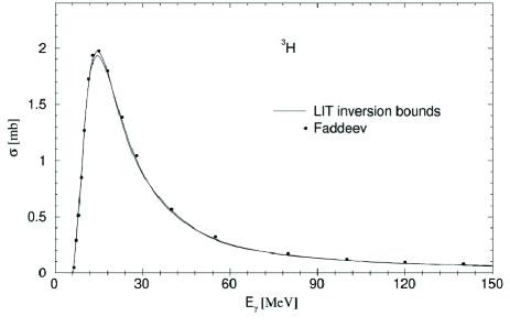
Figure 1: Comparison between Faddeev results (dots) and Lorentz Integral transform (solid lines) in the three-nucleon photodisintegration total cross section with modern realistic two- and three-nucleon forces [29]. The two LIT curves correspond to the small uncertainties in the inversion of the transform (7).

When the comparison is possible, the LIT results have been found in perfect agreement with direct few-body calculations, like the solution of Faddeev-Yakubovsky equations incorporating the full complexity of the continuum states. An example is provided by the three-nucleon photodisintegration cross section displayed in Fig. 1. The results taken from ref. [29] were obtained employing the Argonne AV18 [7] nucleon-nucleon potential and the Urbana UIX [53] three-nucleon force. The LIT case includes also the Coulomb force. Faddeev results are indicated by dots and LIT ones by two curves corresponding to the uncertainties in the inversion of eq.(7). One can see perfect agreement between the two approaches, whereas the uncertainties of LIT method are very small.

The Lorentz Integral Transform represents nowadays the most efficient approach to challenge many-body systems in the continuum. It allows to calculate perturbation induced reaction observables without an explicit use of many-body continuum wave functions. As pointed out in the Introduction, the calculation of these wave functions is made difficult by the existence of many open channels in the continuum, in particular those involving many-body break up reactions. In configuration space calculations the corresponding solutions face the problem of implementing the appropriate boundary conditions. In momentum space, these difficulties are translated into a very complex structure of singularities. In practice exact solutions, in the framework of Faddeev-Yakubovski or AGS equations, are presently limited to A=3 and A=4 systems. The LIT approach therefore constitutes an efficient way to circumvent the boundary condition problem and go well beyond A=4 systems. The interested reader will find a comprehensive review of this approach and a complete reference list in [33].

Although the usual formulation of the LIT method is based on perturbation theory, it can be in principle extended to non perturbative reactions. This possibility was already present in its initial formulation (Sec. 4 of ref. [76]) and has been also emphasized in Sec. 2.3 of a more recent review [33]. Nevertheless, until now, the existing results are however limited to electroweak processes. It would be interesting to demonstrate its applicability to reactions driven by the strong interaction alone, like the simplest elastic $n+^{3}H$ scattering, or neutron induced break-up reactions.

3 Scattering amplitude calculation using continuum-discretized states

As mentioned in the Introduction, the very first idea for using squared integrable basis function to solve the scattering problem was already present in the Wigner’s R-matrix approach, back in the forties [21, 22, 23, 81]. In the nuclear physics community this approach was extensively used to parameterize scattering experiments rather than to compute effectively ab initio scattering observables [24].

The same ideas have been revised from a slightly different perspective, some years later, in a series of papers by Harris starting from ref. [82]. In the simple case of a one channel Schrödinger equation it can be formulated as follows.

We consider the stationary scattering solution of the Schrödinger equation at energy E

$$H\Psi=E\Psi,$$ (8)

in the form

$$\Psi=c_{1}\Psi_{1}(E)+c_{2}\Psi_{2}(E)+\Phi,$$ (9)

where $\Psi_{i}$ are two independent asymptotic solutions at energy E of the free equation and $\Phi$ is an unknown function to be determined, as well as the coefficients $c_{i}(E)$. The scattering observables are obtained from the ratio of these coefficients, in a way depending on the particular choice of the asymptotic solutions $\Psi_{i}$. If, for a three-dimensional solution of the Schrödinger equation, one choses for instance

$$\Psi_{1}=e^{i\vec{k}_{0}\cdot\vec{x}}\qquad\Psi_{2}=\frac{e^{i\mid\vec{k}\mid r}}{r},$$

the ratio would give the scattering amplitude

$$f(\vec{k}_{0}\cdot\vec{k})={c_{2}\over c_{1}}.$$ (10)

The problem remains to determine in an efficient way this ratio and this was the main result in ref. [82]. By inserting (9) into (8) one finds

$$c_{1}(E-H)\Psi_{1}(E)+c_{2}(E-H)\Psi_{2}(E)+(E-H)\Phi=0.$$ (11)

It is worth noticing that, in the asymptotic region, $\Phi$ vanishes only if the coefficients $c_{i}$ are those giving the right asymptotic behavior of the scattering solution. However each of the three terms in equation (11) vanishes in the asymptotic region for arbitrary values of $c_{i}$ . It is then natural to project this equation on a basis of squared integral functions.

Let us denote as $B=\{b_{i}\}_{i=1,\ldots,d}$ a finite basis set, not necessarily orthogonal, and let us diagonalize the Hamiltonian $H$ on this d-dimensional basis by solving the generalized eigenvalue equation

$$(H-\epsilon N)\phi=0,$$

with the d-dimensional matrix

$$H_{ij} = <b_{j}\mid H\mid b_{i}>$$

$$N_{ij} = <b_{j}\mid b_{i}>.$$

The solutions thus obtained ($\epsilon_{n},\phi_{n}$) – assumed by simplicity non degenerate – provides an approximate spectral representation of the Hamiltonian

$$H\approx H^{\prime}=\sum_{n=1}^{d}\mid\phi_{n}>\epsilon_{n}<\phi_{n}\mid,$$

which can be done more and more accurate by increasing the number of states in the basis set.

Let us now project the equation (11) onto one of these eigenvectors $\phi_{m}$

$$c_{1}<\phi_{m}\mid E-H\mid\Psi_{1}(E)>+c_{2}<\phi_{m}\mid E-H\mid\Psi_{2}(E)>+<\phi_{m}\mid E-H\mid\Phi>=0.$$ (12)

The key point of the method is to remark that by choosing E to be the corresponding eigenvalue $\epsilon_{m}$ the term depending on the unknown function $\Phi$ vanishes and one gets

$$c_{1}<\phi_{m}\mid\epsilon_{m}-H\mid\Psi_{1}(\epsilon_{m})>+c_{2}<\phi_{m}\mid\epsilon_{m}-H\mid\Psi_{2}(\epsilon_{m})>=0.$$ (13)

The ratio of the coefficients $c_{i}$ obtained in this way provides an accurate estimation of the scattering amplitude eq.(10) at the energy $E=\epsilon_{m}$, i.e. it is obtained as a ratio of the integral expressions:

$$f(\vec{k}_{0}\cdot\vec{k})={c_{2}\over c_{1}}=-\frac{<\phi_{m}\mid\epsilon_{m}-H\mid\Psi_{1}(\epsilon_{m})>}{<\phi_{m}\mid\epsilon_{m}-H\mid\Psi_{2}(\epsilon_{m})>}.$$ (14)

By interpolating scattering between the ones corresponding to calculated eigenvalues or by adjusting the basis set one can access to an accurate description of the scattering process at any desired energy E. In ref. [82] the method was successfully applied to compute the phase shifts of a two-body problem interacting via a Yukawa potential and in a subsequent work to the scattering of electrons on atomic hydrogen [83]. The method can be in principle generalized to a many-particle system.

Such bound state approach to scattering solutions gained an increasing interest in recent years. They are all based in using the continuum discretize states to obtain the phase shifts at the corresponding energies. In ref. [84] a method was developed that makes use of the Green’s function formalism to obtain the integral representation of the phase shifts in terms of a bound state basis set. It was applied to calculate p-n and n-⁴He scattering observables using semirealistic interactions.

An extension of this approach to coupled channel problems is presented in ref. [85]. The method is based on the introduction of a confining potential in the external region which enables to find a number of independent energy-degenerate solutions corresponding to the number of coupled-channels.

A generalization of the Harris et al. approach and a step further in the complexity of the calculation was achieved in ref. [86]. These authors obtain the scattering amplitude as a ratio of integral expressions like in eq.(14), but they improve this result by taking benefit from the Kohn variational principle [87, 88]. Using a basis of bound-state-like wave functions the scattering matrix corresponding to the n-d (A=3) and p-³He (A=4) scattering was computed for realistic Hamiltonians [86]. This required the extension of the Kohn variational principle to the coupled-channel case. The construction of the energy degenerate bound-state-like wave functions belonging to the continuum spectrum of the Hamiltonian is discussed.

In summary, the method of continuum-discretized states, with several extensions to long range forces and coupled-channel problems, provided already accurate results in systems up to A=4. It has reached now a maturity to be extended in the near future to study more complex systems. Implementation of this method should be straightforward in conjunction with any bound state technique to handle single channel collisions. On the other hand validity of the method should yet be proved for the energies above the three-particle break-up threshold.

4 Complex Scaling Methods in configuration space

The solution of the scattering problem in configuration space is a very difficult task both from formal (theoretical) as well as computational points of view. The principal difficulties arise from the complex asymptotic behavior of the system wave function.

Configuration space wave functions in the asymptotic region combine as many outgoing waves as there are open channels. Moreover, for the break-up channels, which include more than two charged particles, outgoing wave solutions are not even known analytically. The resulting asymptotic form for three-charged particles has been elucidated in ref. [89], however its complexity has discouraged all the efforts to use it explicitly as a boundary condition for solving the Schrö dinger equation. Methods that enable the solution of the scattering problem without using the asymptotic form of the wave function present enormous benefits.

The complex scaling (CS) technique has been introduced already during the World War II by D.R. Hartree et al. [90, 91] in the study of the radio wave propagation in the atmosphere. D.R. Hartree et al. were solving second order differential equations for complex eigenvalues. In practice, this problem is equivalent to the one encountered in the search for resonance positions in quantum two-particle collisions. In the late sixties Nuttal and Cohen [92] proposed a very similar technique to treat the generic scattering problem for short range potentials. Few years later Nuttal even employed this method to solve the three-nucleon scattering problem above breakup threshold [93]. Nevertheless these pioneering works of Nuttal have been mostly forgotten, while based on Nutall’s work and the mathematical foundation of Baslev and Combes [94] the original method of Hartree has been recovered in order to calculate resonance eigenvalues in atomic physics [95, 96]. Such an omission is mostly due to the fact that short range potentials may gain a highly untrivial structure after the complex scaling transformation [97, 98, 99] is applied, while for the Coulomb potential this transformation is trivial.

Only recently a variant of the complex scaling method based on the spectral function formalism has been presented by Katō, Giraud et al. [35, 100, 101] and applied in the works of Katō et al. [35, 36, 37, 38, 39, 40]. This variant will be described in detail in the end of this section. On the contrary in the later works of Kruppa et al. [102] as well as in the works of two of us (J.C. and R.L.) [41, 42] the original idea of Nuttal and Cohen is elaborated.

4.1 Two-body problem

4.1.1 Short range, exponentially bound, interactions

The idea of Nuttal and Cohen [92] can briefly be formulated as follows. The Schrödinger equation is recast into its inhomogeneous (driven) form by splitting the wave function into the sum $\Psi(r)=$ $\Psi^{sc}(r)+\Psi^{in}(r)$, where the incident (free) $\Psi^{in}(\mathbf{r})=\exp(i\mathbf{k}\cdot\mathbf{r})$ wave is separated. The remaining untrivial part of the system wave function $\Psi^{sc}(\mathbf{r})$ describes the scattered waves and may be found by solving a second-order differential equation with an inhomogeneous term:

$$[E-\hat{H_{0}}-V(\mathbf{r})]\Psi^{sc}(\mathbf{r})=V(\mathbf{r})\Psi^{in}(\mathbf{r}).$$ (15)

The scattered wave in the asymptote is represented by an outgoing wave $\Psi^{sc}\sim\exp(ikr)/r,$ where $k=\sqrt{2\mu E}/\hbar$ is the wave number for the relative motion. If one scales all the particle coordinates by a constant complex factor, i.e. $r^{\theta}_{i}=e^{i\theta}r_{i}$ with $Im(e^{i\theta})>0$, the corresponding scattered wave $\overline{\Psi}^{sc}(\mathbf{r})$ will vanish exponentially $\sim\exp(-kr\sin\theta)$ as particle separation $r$ increases. Moreover if the interaction is of short range – exponentially bound with the longest range $\eta^{-1}$ – then after complex scaling the right hand side of eq. (15) also tends to zero at large $r$, if :

$$\tan\theta<\eta/k.$$ (16)

From here we introduce the notation $f^{\theta}(r)=f(re^{i\theta})$ for the complex-scaled functions. The complex scaled driven Schrödinger equation becomes:

$$[E-e^{-i2\theta}\hat{H_{0}}-V^{\theta}(\mathbf{r})]\overline{\Psi}^{sc}(\mathbf{r})=V^{\theta}(\mathbf{r})(\Psi^{in})^{\theta}(\mathbf{r}).$$ (17)

If the condition in eq. (16) is satisfied, the former inhomogeneous equation may be solved by using a compact basis to expand $\overline{\Psi}^{sc}(\mathbf{r})$, thus by employing standard bound-state techniques.

There are two ways to extract scattering information from the obtained solutions $\overline{\Psi}^{sc}(\mathbf{r})$. One method is based on the asymptotic behavior of the outgoing waves, where the scattering amplitude $f_{k}(\hat{r})$ is extracted in a similar way as the asymptotic normalization coefficient from the bound-state wave function, that is, by matching asymptotic behavior of the solution:

$$\overline{\Psi}^{sc}(\mathbf{r})=f_{k}(\widehat{k})e^{-i\theta}\exp(ikre^{i\theta})/r.$$ (18)

The other well known alternative is to use an integral relation which one gets after applying the Green’s theorem [102, 41, 103]:

$$f_{k}(\widehat{k}) = -\frac{2\mu}{\hbar^{2}}e^{i3\theta}\int(\Psi^{in\ast})^{\theta}(\mathbf{r})V^{\theta}(\mathbf{r})\left[\overline{\Psi}^{sc}(\mathbf{r})+(\Psi^{in})^{\theta}(\mathbf{r})\right]d^{3}r$$ (19)

$$= -\frac{2\mu}{\hbar^{2}}e^{i3\theta}\int(\Psi^{in\ast})^{\theta}(\mathbf{r}){V^{\theta}}(\mathbf{r})\overline{\Psi}^{sc}(\mathbf{r})d^{3}r-\frac{2\mu}{\hbar^{2}}\int(\Psi^{in}(\mathbf{r}))^{\ast}V(\mathbf{r}){\Psi}^{in}(\mathbf{r})d^{3}r.$$ (20)

In the second relation one has separated the Born term which may be evaluated without performing complex scaling. The $(\Psi^{in\ast})^{\theta}(\mathbf{r})$ term is obtained by applying the complex-scaling operation on the complex-conjugate function $(\Psi^{in}(\mathbf{r}))^{\ast}$.

4.1.2 Presence of the long range interaction

Let us consider the case where the interaction has an additional long-range term $V(\mathbf{r})=V_{s}(\mathbf{r})+V_{l}(\mathbf{r})$, where $V_{s}(\mathbf{r})$ is exponentially bound and $V_{l}(\mathbf{r})$ is long-ranged. The CS method can be generalized to treat this problem if for the long range term $V_{l}(\mathbf{r})$ the incoming wave solution $\Psi_{l}^{in}(\mathbf{r})$ is analytic and can be extended into the complex r-plane [102, 104, 41]. For the Coulomb case $V_{l}(\mathbf{r})=\frac{\hbar^{2}\eta_{C}}{\mu r}$ the incoming wave solution is well known and is usually expanded in terms of the regular Coulomb functions $F_{\ell}(\eta_{C},kr)$. Then one is left to solve the equivalent driven Schrödinger equation:

$$[E-e^{-i2\theta}\hat{H_{0}}-V^{\theta}(\mathbf{r})]\overline{\Psi}_{s}^{sc}(\mathbf{r})=V^{\theta}_{s}(\mathbf{r})(\Psi_{l}^{in})^{\theta}(\mathbf{r}).$$ (21)

The inhomogeneous term on the right hand side of the former equation is moderated by the short-range interaction term; therefore it is exponentially bound if the condition (16) is fulfilled by the short range potential $V_{s}(\mathbf{r})$.

One may establish a relation equivalent to the eq.(20) in order to determine the long-range-modified short-range interaction amplitude $f_{k,s}(\widehat{k})$ :

$$f_{k,s}(\widehat{k}) = -\frac{2\mu}{\hbar^{2}}e^{i3\theta}\int(\Psi^{in\ast}_{l})^{\theta}(\mathbf{r})V^{\theta}_{s}(\mathbf{r})\overline{\Psi}_{s}^{sc}(\mathbf{r})d^{3}r$$ (22)

$$-\frac{2\mu}{\hbar^{2}}\int(\Psi_{l}^{in}(\mathbf{r}))^{\ast}V_{s}(\mathbf{r}){\Psi}_{l}^{in}(\mathbf{r})d^{3}r.$$

The total scattering amplitude $f_{k}(\widehat{k})$ is a sum of the short-range one and the scattering amplitude due to the long-range term alone $f_{k,l}(\widehat{k})$ :

$$f_{k}(\widehat{k})=f_{k,s}(\widehat{k})+f_{k,l}(\widehat{k}).$$ (23)

4.2 N-body problem

4.2.1 Short range interactions

Here we present the general formalism to treat the collisions of two multiparticle clusters. Lets consider two clusters $a$ and $b$ formed by $N_{a}$ and $N_{b}$ particles (with $N_{a}+N_{b}=N$) whose binding energies are $E_{a}$ and $E_{b}$ respectively. The relative kinetic energy of the two clusters in the center of mass frame is $E_{a,b}=E_{c.m.}-E_{a}-E_{b}=$ $\hbar^{2}k_{a,b}^{2}/2\mu_{a,b}$. Then the incoming wave takes the following form:

$$\Psi_{a,b}^{in}(\mathbf{k}_{a,b},\mathbf{r}_{i,a}\mathbf{,r}_{j,b}\mathbf{,r}_{a,b})=\psi_{a}(\mathbf{r}_{i,a})\psi_{b}(\mathbf{r}_{j,b})\exp(i\mathbf{k}_{a,b}\cdot\mathbf{r}_{a,b}),$$ (24)

where $\psi_{a}(\mathbf{r}_{i,a})$ and $\psi_{b}(\mathbf{r}_{j,b})$ represent bound state wave functions of the clusters $a$ and $b$ respectively, with $\mathbf{r}_{i,a}(\mathbf{r}_{j,b})$ defining internal coordinates of the clusters, while $\mathbf{r}_{a,b}$ is a vector connecting the centers of mass of the two clusters.

As previously, one writes the Schrödinger equation in its inhomogeneous form and applies the complex scaling on all the coordinates, getting:

$$[E-e^{-i2\theta}\hat{H}_{0}-\sum\limits_{m<n}{V^{\theta}_{mn}}\left(\mathbf{r}_{m}\mathbf{-r}_{\mathbf{n}}\right)]\overline{\Psi}_{a,b}^{sc}(\mathbf{r}_{i,a},\mathbf{r}_{j,b}\mathbf{,r}_{a,b})=\left[\sum\limits_{i\in a;j\in b}V^{\theta}_{ij}\left(\mathbf{r}_{i}\mathbf{-r}_{\mathbf{j}}\right)\right](\Psi_{a,b}^{in})^{\theta}(\mathbf{r}_{i,a},\mathbf{r}_{j,b},\mathbf{r}_{a,b}).$$ (25)

The term $\overline{\Psi}_{a,b}^{sc}(\mathbf{r}_{i,a},\mathbf{r}_{j,b},\mathbf{r}_{a,b})$ contains only complex-scaled outgoing waves in the asymptote and thus is formally bound exponentially. Therefore, as long as the right hand side of the last equation is bound, it might be solved using square a integrable basis set to express the scattered part of the wave function $\overline{\Psi}^{sc}_{a,b}(\mathbf{r}_{i,a}\mathbf{,r}_{j,b}\mathbf{,r}_{a,b})$.

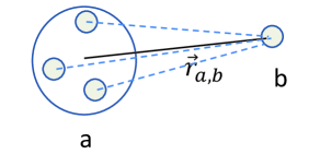
Figure 2: Directions of the interaction terms between the two multiparticle clusters (a and b) do not coincide exactly with the wave vector $\vec{r}_{a,b}$ connecting their centers of mass.

However the inhomogeneous term of eq. (25) is not necessarily exponentially bound even if all the interaction terms are bound. This is due to the fact that, unlike for 2-body case, the directions of the interaction terms do not coincide with the wave vector connecting the center of mass of the two clusters as shown in Fig. 2. Still one may demonstrate that the inhomogeneous term remains bound if an additional condition is fulfilled [41]:

$$\tan\theta<\min(\sqrt{\frac{B_{i\in a}}{E_{a,b}}\frac{m_{i}(M_{a}+M_{b})}{(M_{a}-m_{i})M_{b}}},\sqrt{\frac{B_{j\in b}}{E_{a,b}}\frac{m_{j}(M_{a}+M_{b})}{(M_{b}-m_{j})M_{a}}}),$$ (26)

where $B_{i\in a}$ is the i-th particle removal energy from the cluster $a$ and $M_{a}$ is a total mass of the cluster $a$. The last condition implies additional limit on the complex scaling angle $\theta$ to be used. For a system of equal mass particles this limit does not have much effect and becomes important only well above the break-up threshold $\left|E_{a,b}\right|>>B_{i\in a}$ (or $\left|E_{a,b}\right|>>B_{j\in b}$ respectively). Even at high energies this limit is not so constraining, since the exponent of the scattered wave becomes proportional to $\sqrt{E_{a,b}}$ and therefore one may achieve the same speed of convergence by employing smaller complex scaling angle $\theta$ values. On the other hand the condition in eq. (26) may become strongly restrictive for the mass-imbalanced systems when one considers light-heavy-heavy components.

The scattering observables are easy to calculate using the Green’s theorem. The elastic scattering amplitude is obtained from

$$f_{a,b}(\hat{k}_{a,b}) = -\frac{2\mu}{\hbar^{2}}e^{i3(N-1)\theta}\int({\Psi}_{a,b}^{in\ast})^{\theta}\left[\sum_{i\in a;j\in b}V^{\theta}_{ij}\left(\mathbf{r}_{i}\mathbf{-r}_{\mathbf{j}}\right)\right]\overline{\Psi}_{a,b}^{sc}\prod_{k=1}^{N-1}d^{3}x_{k}$$ (27)

$$-\frac{2\mu}{\hbar^{2}}\int(\Psi_{a,b}^{in})^{\ast}\left[\sum\limits_{i\in a;j\in b}V_{ij}\left(\mathbf{r}_{i}\mathbf{-r}_{\mathbf{j}}\right)\right]\Psi_{a,b}^{in}\prod\limits_{k=1}^{N-1}d^{3}x_{k},$$

where $x_{k}$ represents the internal Jacobi coordinates of the system. Thus one integrates over the full N particle volume by excluding the center of mass one.

Inelastic amplitudes are provided by

$$f_{a,b->c,d}(\widehat{k}_{a,b},\widehat{k}_{c,d}) = -\frac{2\mu}{\hbar^{2}}e^{i3(N-1)\theta}\int({\Psi}_{c,d}^{in^{\ast}})^{\theta}\left[\sum\limits_{i\in c;j\in d}V^{\theta}_{ij}\left(\mathbf{r}_{i}\mathbf{-r}_{\mathbf{j}}\right)\right]\overline{\Psi}_{a,b}^{sc}\prod\limits_{k=1}^{N-1}d^{3}x_{k}$$ (28)

$$-\frac{2\mu}{\hbar^{2}}\int(\Psi_{c,d}^{in})^{\ast}\left[\sum\limits_{i\in c;j\in d}V_{ij}\left(\mathbf{r}_{i}\mathbf{-r}_{\mathbf{j}}\right)\right]\Psi_{a,b}^{in}\prod\limits_{k=1}^{N-1}d^{3}x_{k}.$$

Finally, based on expressions provided in refs. [105, 1], the break-up amplitude into three clusters $(c,d,f)$ is given by:

$$f_{a,b->c,d,f}(\widehat{k}_{a,b},K_{cdf},\widehat{k}_{c,d},\widehat{k}_{cd,f}) = -\frac{2\mu}{\hbar^{2}}e^{i3(N-1)\theta}\int({\Psi}_{c,d,f}^{in\ast})^{\theta}{V_{cdf}^{\theta}}\overline{\Psi}_{a,b}^{sc}\prod\limits_{k=1}^{N-1}d^{3}x_{k}$$ (29)

$$-\frac{2\mu}{\hbar^{2}}\int(\Psi_{c,d,f}^{in})^{\ast}V_{cdf}\Psi_{a,b}^{in}\prod\limits_{k=1}^{N-1}d^{3}x_{k}.$$

In the last equation the interaction term is

$$V_{cdf}=\sum_{i<j}V_{ij}-\sum_{(m<k)\in c}V_{mk}-\sum_{(m<k)\in d}V_{mk}-\sum_{(m<k)\in f}V_{mk}.$$ (30)

4.2.2 Presence of the long range interaction

One may try to include the long-range interaction in a similar manner as it has been done for the 2-body case. To this aim one should separate the incoming wave $\left(\Psi_{a,b}^{in}\right)_{l}$ modified by the residual long-range interaction term $V_{l}(\mathbf{r}_{a,b})$. In particular, for the charged projectile-target system it is natural to subtract the residual Coulomb interaction between the colliding clusters $a$ and $b$ with $V_{l}(\mathbf{r}_{a,b})=Z_{a}Z_{b}/\mathbf{r}_{a,b}$, where $Z_{a}$ and $Z_{b}$ are respective charges of the projectile and target respectively.

$$[E-e^{-i2\theta}\hat{H}_{0}-\sum\limits_{m<n}{V_{mn}^{\theta}}\left(\mathbf{r}_{m}\mathbf{-r}_{\mathbf{n}}\right)]\left({\Psi}_{a,b}^{sc}\right)_{l}(\mathbf{r}_{i,a}\mathbf{,r}_{j,b}\mathbf{,r}_{a,b})=\left[\sum\limits_{i\in a;j\in b}{V_{ij}^{\theta}}\left(\mathbf{r}_{i}\mathbf{-r}_{\mathbf{j}}\right)-{V_{l}^{\theta}}(\mathbf{r}_{a,b})\right]{\left(\Psi_{a,b}^{in}\right)^{\theta}_{l}}(\mathbf{r}_{i,a}\mathbf{,r}_{j,b}\mathbf{,r}_{a,b}).$$ (31)

However the residual interaction term $\left[\sum\limits_{i\in a;j\in b}{V_{ij}^{\theta}}\left(\mathbf{r}_{i}\mathbf{-r}_{\mathbf{j}}\right)-{V_{l}^{\theta}}(\mathbf{r}_{a,b})\right]$, appearing on the right hand side of this equation, still retains some higher-order terms which may not converge exponentially. In particular, for the aforementioned case of the charged clusters (Coulomb case) this interaction term retains higher order Coulomb multipolar terms starting with $1/r_{a,b}^{3}$, which are due to the possible polarization of the projectile-target. Therefore the right-hand side of the last equation is not exponentially bound but contains long-range slowly diverging terms. Nevertheless these multipolar terms are weak, even compared to the subtracted long-range interaction term (as discussed for $Z_{a}Z_{b}/\mathbf{r}_{a,b}$ Coulomb case) and should represent only mild corrections in the far asymptote region. Therefore if a system is dominated by the strong short-range interaction terms one might eventually consider screening these multipolar terms due to the residual long-range interaction. Such a procedure is used in obtaining the results presented in the next section for three-body systems interacting via Coulomb plus short-range nuclear potentials finding no consequences on the final result.

4.2.3 External probes

There is a group of problems in physics where the system is initially in a bound state and gets subsequently excited to the continuum by an external source that is considered as a perturbation. In particular, it concerns reactions led by electro-magnetic and weak probes. In this case one is interested in evaluating the strength or response function given in lowest order perturbation theory as

$$S(E)=\sum_{\nu}\left|\left\langle\Psi_{\nu}\left|\widehat{O}\right|\Psi_{0}\right\rangle\right|^{2}\delta(E_{\nu}-E_{0}-E),$$ (32)

where $\hat{O}$ is the perturbation operator which induces the transition from the bound-state $\Psi_{0},$ with ground-state energy $E_{0}$, to the state $\Psi_{\nu}$ with energy $E_{\nu}$. Both wave functions are solutions of the same Hamiltonian $H$ . The energy is measured from some standard value, e.g., a particle-decay threshold energy. When the excited state is in the continuum, the label $\nu$ is continuous and the sum must be replaced by an integration. Furthermore the final state wave function $\Psi_{\nu}$ may have complicate asymptotic behavior in configuration space if it represents continuum states. On the other hand the expression may  be rewritten by avoiding summation over the final states

$$S(E) = \left\langle\Psi_{0}\left|\widehat{O}^{{\dagger}}\delta(H-E_{\nu})\widehat{O}\right|\Psi_{0}\right\rangle$$ (33)

$$= -\frac{1}{\pi}Im\left\langle\Psi_{0}\left|\widehat{O}^{{\dagger}}G(E_{\nu}+i\varepsilon)\widehat{O}\right|\Psi_{0}\right\rangle=-\frac{1}{\pi}Im\left\langle\Psi_{0}\left|\widehat{O}^{{\dagger}}\right|\Phi_{\nu}\right\rangle$$ (34)

with

$$(H-E_{\nu})\Phi_{\nu}=\widehat{O}\Psi_{0}.$$ (35)

The right hand side of the former equation is compact, damped by the bound-state $\Psi_{0}$ wave function. The wave function $\Phi_{\nu}$ asymptotically contains only outgoing waves. Therefore the last inhomogeneous equation may be readily solved using complex scaling techniques

$$(H^{\theta}-E_{\nu})\overline{\Phi}_{\nu}=\widehat{O}^{\theta}\Psi_{0}^{\theta}.$$ (36)

One must just use the complex scaled expressions for the right hand side of the equation. The complex-scaled bound state wave function $\Psi_{0}^{\theta}$ is obtained by solving the bound state problem using the complex-scaled Hamiltonian

$$(H^{\theta}-E_{0})\Psi_{0}^{\theta}=0,$$ (37)

and finally

$$S(E)=-\frac{1}{\pi}Im\left\langle\Psi_{0}^{\theta}\left|(\widehat{O}^{{\dagger}})^{\theta}\right|\overline{\Phi}_{\nu}\right\rangle.$$ (38)

4.2.4 Complex scaled Green’s function method

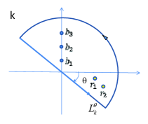
Figure 3: The Cauchy integral contour in the momentum plane for the completeness relation of the complex scaled Hamiltonian. The $b_{1},b_{2},..$ and $r_{1},r_{2},..$ represent the bound and resonant poles respectively.

A slightly different procedure to obtain the physical solution of the complex scaled Hamiltonian has been proposed by Katō, Giraud et al. [35, 100, 101]. In the last paper the completeness relation of the Berggren [106] has been proved for the complex scaled Hamiltonian solutions representing bound, resonant as well as single- and coupled-channel scattering states. This completeness relation can be formulated for the Cauchy integral contour in the momentum plane as demonstrated in fig. 3, as:

$$\mathbf{1}=\sum_{B}\left|\chi_{B}^{\theta}\right)\left(\chi_{B}^{\theta}\right|+\sum_{R}^{n_{R}^{\theta}}\left|\chi_{R}^{\theta}\right)\left(\chi_{R}^{\theta}\right|+\int_{L_{k}^{\theta}}dk_{\theta}\left|\chi_{k_{\theta}}\right)\left(\chi_{k_{\theta}}\right|,$$ (39)

here $\chi_{B}^{\theta}$ and $\chi_{R}^{\theta}$ are the complex scaled bound and resonant state wave-functions respectively. Only the resonant states encircled by the semicircle rotated by angle $\theta$ must be considered. The remaining continuum states $\chi_{k}^{\theta}$ are located on the rotated momentum axis $L_{k}^{\theta}$ (see Fig. 3). One should mention that the definition of the complex scaled bra- and ket-states for the non-Hermitian $H^{\theta}$ are different from the usual ones of the Hermitian Hamiltonian. For $H^{\theta}$ one expresses the bra-state as the bi-conjugate solution of the ket-state. In practice, for the discrete (resonant and bound) states we can use the same wave functions for the bra- and ket-states; for the continuum states the wave function of the bra-state is given by that of the ket-state divided by the S-matrix. This is the reason we use different notation to designate the complex scaled bra- and ket-states $\left|\chi^{\theta}\right)$, instead of the commonly accepted notation $\left|\chi\right>$ for solutions of Hermitian Hamiltonians.

Using the former completeness relation, the complex scaled Green’s function is written

$$\mathcal{G^{\theta}}(E,\mathbf{r},\mathbf{r^{\prime}})=\sum_{B}\frac{\left|\chi_{B}^{\theta}(\mathbf{r})\right)\left(\chi_{B}^{\theta}(\mathbf{r^{\prime}})\right|}{E-E_{B}}+\sum_{R}^{n_{R}^{\theta}}\frac{\left|\chi_{R}^{\theta}(\mathbf{r})\right)\left(\chi_{R}^{\theta}(\mathbf{r^{\prime}})\right|}{E-E_{R}}+\int_{L_{k}^{\theta}}dk_{\theta}\frac{\left|\chi_{k_{\theta}}(\mathbf{r})\right)\left(\chi_{k_{\theta}}(\mathbf{r^{\prime}})\right|}{E-E_{\theta}},$$ (40)

where $E_{B}$ and $E_{R}=(E_{r}-\frac{i}{2}\Gamma)$ are the energy eigenvalues of the bound and relevant resonant states respectively. Variables $\mathbf{r}$ reflect all the internal coordinates of the multiparticle system under consideration. By plugging the last relation into the eq. (34), one finally gets:

$$S(E) = S_{B}(E)+S^{\theta}_{R}(E)+S^{\theta}_{k}(E),$$ (41)

$$S_{B}(E) = -\frac{1}{\pi}Im\sum_{B}\frac{\left(\Psi_{0}^{\theta}\right|(\widehat{O}^{\dagger})^{\theta}\left|\chi_{B}^{\theta}\right)\left(\chi_{B}^{\theta}\right|\widehat{O}^{\theta}\left|\Psi_{0}^{\theta}\right)}{E-E_{B}},$$ (42)

$$S^{\theta}_{R}(E) = -\frac{1}{\pi}Im\sum_{R}^{n_{R}^{\theta}}\frac{\left(\Psi_{0}^{\theta}\right|(\widehat{O}^{\dagger})^{\theta}\left|\chi_{R}^{\theta}\right)\left(\chi_{R}^{\theta}\right|\widehat{O}^{\theta}\left|\Psi_{0}^{\theta}\right)}{E-E_{R}},$$ (43)

$$S^{\theta}_{k}(E) = -\frac{1}{\pi}Im\int_{L^{\theta}_{k}}\frac{\left(\Psi_{0}^{\theta}\right|(\widehat{O}^{\dagger})^{\theta}\left|\chi_{k_{\theta}}\right)\left(\chi_{k_{\theta}}\right|\widehat{O}^{\theta}\left|\Psi_{0}^{\theta}\right)}{E-E_{\theta}}.$$ (44)

In practice (numerical solution) one works with a finite basis; then the last term containing the integration is replaced by the sum running over all the complex eigenvalues representing continuum pseudo states. All the eigenvalues are obtained as solutions of the complex scaled Hamiltonian with a pure outgoing wave boundary condition (i.e. exponentially converging ones due to complex scaling).

The obtained total strength function $S(E)$ should be independent of the angle $\theta$ employed in the calculation. Furthermore the strength function component $S_{B}(E)$, as well as its partial components due to separate bound states are also independent of $\theta$. The partial components of $S^{\theta}_{R}(E)$, corresponding the same narrow resonance, also turn out to be independent of $\theta$ as long as the angle $\theta$ is large enough to encircle this resonance. However if the resonance is large enough and is not encircled by the contour $L^{\theta}_{k}$, its contribution to the strength function is reabsorbed by the pseudo-continuum states in the $S^{\theta}_{k}(E)$ term. This feature has been clearly demonstrated in ref. [37] for a chosen 2-body example.

Relation (43) offers an unique feature to separate the contributions of the resonant and bound states in the strength function. The contributions of the narrow resonances should not depend on the angle $\theta$, if the angle $\theta$ is large enough to encircle a considered resonance.

Figure 4: (Color online) Schematic representation of the eigenvalues of the complex scaled Hamiltonian, $H^{\theta}$ , according to the theorem of Balslev and Combes [94]. For a two-body system (left-pane) bound states are obtained as negative real energy eigenvalues, continuum-pseudostates are rotated by angle $2\theta$, resonances inside $2\theta$ branch may also be obtained. For a many-body system (right pane) several rotated continuum branches exist associated with bound and resonant subcluster thresholds.

For the sake of simplicity, the contour depicted in the Fig. 3 represents the simplest 2-body case. Still all of the relations presented remain valid for the many-body system; one only should keep in mind that the obtained spectra may have a much more complicated structure. Following the Balslev and Combes theorem [94] the eigenvalues of the complex-scaled two-body Hamiltonian, which are associated with the bounded wave function, splits into three categories: bound state eigenvalues situated on the negative horizontal energy axis, pseudo-continuum states scattered along the positive energy axis rotated by angle $2\theta$ and some eigenvalues representing the resonances whose eigen energies satisfy the relation -$arg(E)<2\theta$ (see left plane of Fig. 4). For the many-body system bound states will be situated on the horizontal part of the energy axis, situated below the lowest system separation into multiparticle cluster threshold (see Fig. 4). Pseudo-continuum states will scatter along the $2\theta$-lines projected from each possible separation threshold. In addition one will have $2\theta$-lines projected from the ”resonant thresholds”, where one or more sub-cluster is resonant. Finally, many-body resonance eigenvalues will represent discrete points inside the semicircle making angle $2\theta$ with the real energy axis and derived from the lowest threshold.

4.3 Scattering amplitude via Greens-function method

The first application of the CS Green’s function method to calculate scattering phaseshifts has been realized by using the continuum level density (CLD) formalism. One starts with the CLD definition as

$$\Delta(E)=-\frac{1}{\pi}\textrm{Im}\left(\textrm{Tr}[G(E)-G_{0}(E]\right),$$ (45)

with $G(E)=(E-H)^{-1}$ and $G_{0}(E)=(E-H_{0})^{-1}$ being full and free Green’s functions, respectively. In principle, the former expression may be generalized to the scattering of two complex clusters. Then $H_{0}$, besides the kinetic energy, should include interactions inside separate clusters, whereas $H$ includes all the interaction terms in the two-cluster system. Thus CLD expresses the effect from the interactions connecting the two clusters. When the eigenvalues of $H$ and $H_{0}$ are obtained approximately ($\epsilon_{i}$ and $\epsilon^{0}_{i}$ respectively) within the framework of including a finite number of the basis functions (N), the discrete CLD is defined:

$$\Delta(E)_{N}=\sum_{i}\delta(E-\epsilon_{i})-\sum_{j}\delta(E-\epsilon^{0}_{j}).$$ (46)

The CLD is related to the scattering phaseshift

$$\Delta(E)=\frac{1}{\pi}\frac{d\varphi(E)}{dE},$$ (47)

and thus one can inversely calculate the phaseshift ($\varphi$) by integrating the last equation obtained as a function of energy. These equations are difficult to apply for real Hamiltonians, as one will necessarily confront the singularities present in eq. (45-46). However by using CS expressions for the Green’s functions, these singularities are avoided and replaced by smooth Lorentzian functions. By plugging in CS Green’s function expression (40) into (46) and after some simple algebra one gets:

$$\Delta(E)_{N}=\overline{\rho}_{N}^{\theta}(E)-\rho_{N}^{(0)\theta}(E)$$ (48)

and

$$\overline{\rho}_{N}^{\theta}(E)=\frac{1}{\pi}\sum_{R}^{n_{R}^{\theta}}\frac{1}{(E-E_{R})}+\frac{1}{\pi}\sum_{k}^{N-n_{R}^{\theta}-n_{B}}\frac{1}{(E-E^{\theta}_{k})}.$$ (49)

In the last expression $E_{R}$ and $E^{\theta}_{k}$ are the eigenvalues of the full CS Hamiltonian $H^{\theta}$ representing resonant and continuum states respectively. One should pay attention that the sum over bound-states in the last expression is dropped. The term $\rho_{N}^{(0)\theta}$ is equivalent to $\overline{\rho}_{N}^{\theta}(E)$ obtained for the CS free Hamiltonian $H_{0}^{\theta}$; this term contains only pseudo-continuum states aligned along $2\theta$-lines pointing out from the scattering thresholds (see Fig. 4).

There exists however a much more straightforward way to calculate scattering observables using CS Green’s function [102]. Indeed, as one may see in eqs. (27-29), the scattering amplitude naturally splits into the Born (trivial) and the remaining (untrivial) term. The Born term may be calculated only knowing the bound state wave functions of the incident and outgoing subsystems. The nontrivial part of the scattering amplitude requires knowledge of the CS scattered wave function $\overline{\Psi}_{a,b}^{sc}$ at a given scattering energy $E$. This part of the system wave-function is easily expressed using the CS Green’s function of eq. (40):

$$\overline{\Psi}_{a,b}^{sc}(r)=\int d^{3}r^{\prime}\mathcal{G^{\theta}}(E,\mathbf{r},\mathbf{r^{\prime}})({\Psi}_{a,b}^{in})^{\theta}(r^{\prime}),$$ (50)

where r and r’ are all the internal coordinates in the n-body system.

As demonstrated in ref. [102], the two approaches, the one presented in subsection 4.2.1 based on the solution of differential equations with an inhomogenious term and the one based on CS Green’s function via equations (47-49), are fully equivalent. I.e., if one employs the same numerical technique to solve the differential equations with an inhomogenious term of the type shown in eq. (25) or one calculates eigenvalues of the respective $H^{\theta}$ to approximate the CS Green’s function in eq.(40), one will find identical values for the scattering amplitude. On the contrary, the CLD procedure to extract the scattering phaseshifts (or the amplitude eventually) is not fully equivalent. Based on our limited experience in the 2-body sector we found that the scattering phaseshifts calculated using expressions (40) and (50), are more accurate than those obtained through expressions (47) through (49) based on CLD formalism.

It should be noted that a full spectral decomposition of $H^{\theta}$ is required to express CS Green’s function in eq. (40) and to evaluate the scattering amplitudes. The scattering amplitude, except in the case of resonant scattering, is not determined by one or a few dominant eigenvalues. This may turn out to be a crucial obstacle in applying CS Green’s function method in studying many-body systems, since the resulting algebraic eigenvalue problem becomes too large to be fully diagonalised. In this case the original prescription of Nuttall, described in the subsection 4.2.1, turns out to be strongly advantageous. The last prescription resides on a single solution of a linear-algebra problem, allowing one to employ the iterative methods (without explicit storage of the matrix elements) to solve a resulting large-scale problem.

On the other hand the CS Green’s function formalism provides a clear physical interpretation of the scattering observables in terms of bound, resonant and continuum states. Furthermore, the same CS Green’s function expression is used to describe both collision processes as well as system response to different perturbations (like systems response to EM or weak field), thus providing a solid ground to study correlations between different physical observables.

Finally, one should discuss some technical aspects of the CS method, which may hamper its successful implementation. First CS implies complex arithmetics and non-Hermitian matrices already for the problems involving only binary scattering channels. However some linear-algebra methods used in numerical calculations are limited to real Hermitian matrices. In the CS method one works with the analytical potentials extended to the complex r-plane. However, as pointed out in refs. [97, 98, 99] not all the potentials behave well under complex scaling. In particular, short-range potentials become oscillatory and even start diverging for large $\theta$ values. Therefore, in numerical calculations it is advisable to keep the angle $\theta$ values small to guarantee the smoothness of the potential after complex scaling in order to allow the numerical treatability of the problem [98, 99]. On the other hand the far asymptote of the complex-scaled outgoing wave solution is proportional to $exp(-k_{x}r_{x}\sin{\theta})$, where $k_{x}$ is a wave vector corresponding to the last open-channel (channel with the lowest free energy for the reaction products). Thus large angle $\theta$ values are required to damp efficiently outgoing wave solution if calculations are performed close to the threshold (small $k_{x}$ value). This last fact makes it difficult to use CS in exploring energy regions close to open thresholds.

4.4 Results

McDonald and Nuttall were the first to apply the complex scaling method to treat the scattering problem in $A>2$ system, already back in 1972. They have studied neutron-deuteron scattering at neutron laboratory energies up to 24 MeV. Nucleon-nucleon interaction in spin singlet and triplet channels has been described by a single Yukawa-term potential, whose parameters have been adjusted to reproduce the low-energy two-nucleon observables: deuteron binding energy, singlet and triplet scattering length as well as singlet effective range. Regardless of the simplicity of the employed interaction, McDonald and Nuttall have managed to point out the great difference in doublet and quartet inelastic parameters, in particular demonstrating that the deuteron resists to breakup in the quartet channel. Furthermore strong sensitivity of the doublet channel to the nature of the NN-interaction has been revealed. The calculated neutron-deuteron scattering length in the doublet channel, however, turned out to be too large, as a result of the strongly overbound triton. This effect is undoubtedly due to the softness of the employed NN interaction. In spite of these rather encouraging results, the developments of McDonald and Nuttall have stopped.

Only in the late nineties has the complex scaling method been revisited for scattering calculations while trying to apply it to Coulombic systems [108, 109, 110]. Still, due to the dominance of the long-range interaction, the direct approach described above does not hold and thus a variant based on the exterior complex scaling has been developed [111]. One should mention however that it is extremely difficult to apply the exterior complex scaling method to non-central or non-local interactions [111] as encountered in nuclear physics.

Figure 5: Strength distribution of the E1 disintegration of ${}^{6}He$ nucleus. In the left pane model results [37] are compared with the experimental data of [112] using a secondary ${}^{6}He$ ion beam of 240 MeV/nucleon incident on carbon and lead targets. The calculated cross section is convoluted with respect to experimental data. In the right pane the total strength (full line) is split into contribution of two-body and three-body channels.

Interest in the CS method vis-$\grave{\rm{a}}$-vis nuclear reactions has been revived by the work of Katō et al. [35, 100, 101]. The method based on the spectral decomposition described in section 4.2.4 has been applied by Katō et al. [36, 37] mostly in analyzing the EM response of two-neutron halo nuclei. In particular, E1 and E2 Coulomb breakup of ⁶He and ¹¹Li nuclei has been studied, using a semi-microscopical three-body model. In such a model ⁶He or ¹¹Li nuclei are represented by two neutrons attached to the ⁴He or ⁹Li cores respectively. The core cluster (⁴He or ⁹Li) is considered to be in its ground state, and only the interactions between the two halo neutrons and halo neutron-core are explicitly considered. The three-body wave function is antisymmetric with respect to the last two neutrons. The Pauli principle between the core and halo neutrons is mimicked using the orthogonality condition model through the pseudo-potential method of Kukulin et al. [113]. In Fig. 5 the strength distribution of the E1 transition for ⁶He, as obtained in ref. [37], is presented. In the last calculation the microscopic KKNN potential [114] and the effective Minnesota potential [115] have been used to represent $V_{{}^{4}He-n}$ and $V_{n-n}$ interactions, respectively. Such a simplistic model allows a rather accurate description of the experimental data. Furthermore, from the obtained results one may conclude the dominance of the sequential ${}^{6}\textrm{He}\rightarrow^{5}\textrm{He +n}\rightarrow^{4}\textrm{He +n +n}$ process in the Coulomb breakup of ${}^{6}\textrm{He}$. This reaction proceeds mostly through $J=3/2^{-}$ and $J=1/2^{-}$ resonances of ${}^{5}\textrm{He}$. This demonstrates the importance of the CS Green’s function method, which provides a clear physical interpretation of the scattering observables in terms of bound, resonant and continuum states.

In a later work by the same group of Japanese scientists [40] the EM breakup of ${}^{11}\textrm{Li}$ has been studied in an extended three-body model, by representing ${}^{9}\textrm{Li}$ core as a coupled cluster including $2p-2h$ excitations.

In ref. [39] the aforementioned three-body model has also been used to study deuteron elastic scattering on ${}^{4}\textrm{He}$ as well as ${}^{2}\textrm{H}(^{4}\textrm{He},\gamma)^{6}\textrm{Li}$ radiative capture reaction.

On the contrary, in the studies by two of us (R.L. and J.C.) [41, 42], the original complex scaling method of Nuttall and Cohen, described in section  4.2.1, is elaborated. The few-body problem is solved for the complex scaled Faddeev-Yakubovski equations. In particular the validity of the CS method has been demonstrated for n+${}^{2}\textrm{H}$ scattering above the deuteron breakup threshold, by comparing results with the ones obtained using direct configuration and momentum space methods [41]. Furthermore the validity of the CS method has been demonstrated for systems which interact via optical potentials that have an absorbing-imaginary part [43, 44]. As a test case, the n+p+¹²C system has been considered within a three-body model. In this system the n-p interaction was described using the realistic AV18 model [7]. The interaction between the neutron (proton) and the ¹²C core was simulated by the optical potential [116]. Elastic p$+^{13}$C, d+¹²C as well as inelastic p$+^{13}$C$\rightarrow$d$+^{12}$C cross sections have been calculated for 30 MeV deuteron (or 30.6 MeV proton) laboratory energy, which is above n+p+¹²C breakup threshold. Excellent agreement with a direct momentum space calculations based on AGS equations and the Coulomb-screening method [16], has been obtained.

Lately the CS method has been applied to solve the four-nucleon scattering problem [42] for total isospin $T=0$ and $T=1$ channels. S-wave spin-dependent MT I-III potential was employed to mimic the nucleon-nucleon interaction but ignoring the Coulomb repulsion between the protons. The four-nucleon system has been studied both above 3-body (the N+N+(NN) case) and 4-body (N+N+N+N) breakup thresholds. Results have been compared with the ones obtained using momentum space complex-energy method giving excellent agreement. Reasonable agreement with the experimental data of refs. [117, 118, 119] has been found for n+³H scattering above the 4-body breakup threshold as shown in Fig. 6. Even better description of the experimental data can be found if realistic interactions are used, as pointed out in ref. [65]. The isospin $T=0$ channel has been found to be very sensitive to the nucleon-nucleon interaction input and thus requires a more realistic model in order to reproduce the experimental data.

Figure 6: Calculated n+³H elastic differential cross-sections for neutrons of lab. energy 14.4 MeV (left pane) and 22.1 MeV (right pane) compared with the experimental results of Frenje et al. [117], Debertin et al. [118] and Seagrave et al. [119].

5 Complex energy method in configuration space

Effective range theory is one of the most popular tools in analyzing and describing scattering processes. This fact clearly indicates that analytical continuation methods can be successfully applied to circumvent the well-known difficulties in solving scattering problems. Already in the mid-sixties Schlessinger and Schwartz [120] proposed a continuation method to calculate the elastic scattering amplitude from the results obtained in the negative energy region. The idea of Schlessinger has been generalized to complex energy by McDonald and Nuttall [121]. The starting point for this method is the inhomogeneous Scrödinger equation:

$$[E_{c}-\hat{H}_{0}-\sum\limits_{m<n}{V_{mn}}\left(\mathbf{r}_{m}\mathbf{-r}_{\mathbf{n}}\right)]\overline{\Psi}_{a,b}^{sc}(E_{c},\mathbf{r}_{i,a},\mathbf{r}_{j,b}\mathbf{,r}_{a,b})=\left[\sum\limits_{i\in a;j\in b}V^{\theta}_{ij}\left(\mathbf{r}_{i}\mathbf{-r}_{\mathbf{j}}\right)\right]\Psi_{a,b}^{in}(E^{\prime}_{c},\mathbf{r}_{i,a},\mathbf{r}_{j,b},\mathbf{r}_{a,b}).$$ (51)

One solves this equation for a complex energy $E_{c}=|E_{c}|e^{2i\theta}$ with a positive imaginary part (i.e. $\theta<\pi/2$). The last condition on the angle $\theta$ allows to avoid the cut along the real-energy axis, while the outgoing wave solutions $\overline{\Psi}_{a,b}^{sc}(E_{c},\mathbf{r}_{i,a},\mathbf{r}_{j,b}\mathbf{,r}_{a,b})$ fall exponentially at large distances. One may use integral relations formulated in subsection 4.2.1 in order to evaluate scattering amplitudes for complex energies in the upper half-plane. Physical amplitudes, corresponding the real energy values, might be extrapolated from the amplitude values obtained for the complex energies.

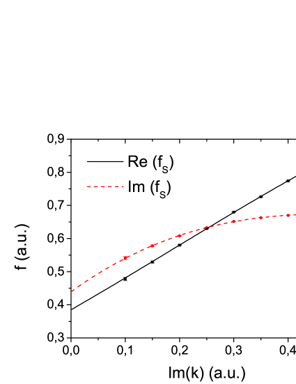
Figure 7: Electron scattering on hydrogen atom in its ground state at $Re(k)=1.103$ a.u. Scattering amplitude dependence on the imaginary part of the momenta. Calculated points by McDonald and Nuttall [121] are fitted using third order polynomial function.

Formally there is the liberty to choose the energy mapping $E^{\prime}_{c}(E_{c})$ between the incoming wave and scattered wave terms, as long as it allows one to perform extrapolation to the real energy axis. Obviously it should be a smooth function with the formal requirement that the real energies are not affected by the mapping, i.e. $E^{\prime}_{c}(Re(E_{c}))=Re(E_{c})$. Two natural choices exist for the mapping function, namely $E^{\prime}_{c}(E_{c})=E_{c}$ and $E^{\prime}_{c}(E_{c})=Re(E_{c})$. In the pioneering work of McDonald and Nuttall [121] the three-body Coulomb problem was considered; therefore the second relation has been chosen in order to avoid divergence of the inhomogeneous term in eq. (51). However the convergence of the inhomogeneous term may be also provided by exponentially-bound interactions. Based on our limited experience studying the 2-body system we have found that the extrapolation procedure is more stable using the $E^{\prime}_{c}(E_{c})=E_{c}$ mapping.

In Fig. 7 we present the behavior of the spin-singlet amplitude as a function of the imaginary part $Im(k)$ of the momentum for electron scattering on hydrogen atom in its ground state at $Re(k)=1.103$ a.u.. These calculations have been performed by McDonald and Nuttall in their pioneering works [121, 122] on the complex-energy method. At that time the numerical solution of the full three-body problem was beyond the technical means and the scattering amplitude was estimated to second order from the variational principle of Schlessinger  [123]. We may see a smooth amplitude dependence on the complex momentum, thus enabling easy extrapolation to real momentum value. In Fig. 7 a third order polynomial fit is used, providing an extrapolated value $f_{S}=0.365(14)+0.440(14)i$ in full agreement with the result of McDonald and Nuttall using rational fraction fitting procedure.

The developments of McDonald and Nuttall [121, 122] based on the complex energy method have not been pursued in configuration space. Nevertheless this method has been revived recently by developments in momentum space. The momentum space complex-energy method is presented in the next section.

6 Complex energy method in momentum space

As shown in previous sections, if one uses differential equations in coordinate space for the description of few-particle scattering processes, one is faced with nontrivial asymptotic boundary conditions when the channels with three or more clusters become energetically open. In the framework of momentum-space integral equations this gives rise to integral kernels with a very complicated structure of singularities. Furthermore, the complexity of the singularities increases with the number of particles (likewise the complexity of the wave function asymptotic form in configuration space). Formally, this difficulty can be avoided by applying the complex energy method of ref. [121, 122] described in a previous chapter to momentum space calculations [124]. The complex energy parameter used to damp outgoing waves in configuration space calculations serves to smoothen integral kernel singularities present in momentum space calculations. Using such a direct momentum-space approach the neutron-deuteron scattering with simple model potentials was calculated in refs. [124, 125].

Nevertheless, only for sufficiently large complex energy parameter the integral equation kernels become smooth enough to be integrated without special care. On the other hand, in the three-particle system the complex energy method seems to be unnecessary. Indeed, the most sophisticated momentum-space calculations of neutron-deuteron [126, 127, 3] and proton-deuteron [15, 16, 128] elastic scattering and breakup and of three-body nuclear reactions [71, 73] are done directly at real energies using real-axis integration methods; thus, the integral equation kernel singularities in the three-particle system are well under control. In contrast, the only existing momentum-space calculations for the scattering of four particles above four-particle breakup threshold are done using the complex energy method. First four-nucleon scattering calculations were presented in ref. [64]; however, they employed simple separable potentials. Only very recently fully realistic four-nucleon scattering calculations using modern nuclear interactions and including the proton-proton Coulomb force have been performed [65, 129, 66]. Important refinements of the complex energy method were developed to improve its accuracy and practical applicability, given the need to include a large number of partial waves in realistic calculations. In this section the complex energy method with emphasis on these special developments is summarized. The four-nucleon system is employed to illustrate the method.

Four-nucleon scattering process may be described exactly using the Alt, Grassberger, and Sandhas (AGS) equations [46] for the symmetrized four-particle transition operators $\mathcal{U}_{\beta\alpha}$ as derived in ref. [56], where the nucleons are treated as identical particles in the isospin formalism, i.e.,

$$\mathcal{U}_{11}={} \eta(G_{0}\,t\,G_{0})^{-1}P_{34}+\eta P_{34}U_{1}G_{0}\,t\,G_{0}\,\mathcal{U}_{11}+U_{2}G_{0}\,t\,G_{0}\,\mathcal{U}_{21},$$ (52a)

$$\mathcal{U}_{21}={} (G_{0}\,t\,G_{0})^{-1}(1+\eta P_{34})+(1+\eta P_{34})U_{1}G_{0}\,t\,G_{0}\,\mathcal{U}_{11},$$ (52b)

$$\mathcal{U}_{12}={} (G_{0}\,t\,G_{0})^{-1}+\eta P_{34}U_{1}G_{0}\,t\,G_{0}\,\mathcal{U}_{12}+U_{2}G_{0}\,t\,G_{0}\,\mathcal{U}_{22},$$ (52c)

$$\mathcal{U}_{22}={} (1+\eta P_{34})U_{1}G_{0}\,t\,G_{0}\,\mathcal{U}_{12}.$$ (52d)

Here, $\eta=-1$ (+1) for identical fermions (bosons), $\alpha=1$ corresponds to the $3+1$ partition (12,3)4 whereas $\alpha=2$ corresponds to the $2+2$ partition (12)(34); there are no other distinct two-cluster partitions in the system of four identical particles. The energy dependence of the operators arises from the free resolvent

$$G_{0}=(Z-H_{0})^{-1}$$ (53)

with the complex energy parameter $Z=E+i\varepsilon$ and the free Hamiltonian $H_{0}$, while

$$t=v+vG_{0}t$$ (54)

is the pair (12) transition matrix derived from the potential $v$, and

$$U_{\alpha}=P_{\alpha}G_{0}^{-1}+P_{\alpha}t\,G_{0}\,U_{\alpha}$$ (55)

are the symmetrized 3+1 or 2+2 subsystem transition operators. For the four-nucleon system the basis states are antisymmetric under exchange of two particles in the subsystem (12), and, in the $2+2$ partition, also in the subsystem (34). The full antisymmetry is ensured by the permutation operators $P_{ab}$ of particles $a$ and $b$ with $P_{1}=P_{12}\,P_{23}+P_{13}\,P_{23}$ and $P_{2}=P_{13}\,P_{24}$.

The scattering amplitudes for two-cluster reactions at available energy $E=\epsilon_{\alpha}+p_{\alpha}^{2}/2\mu_{\alpha}=\epsilon_{\beta}+p_{\beta}^{2}/2\mu_{\beta}$ are obtained from the on-shell matrix elements $\langle{\mathbf{p}}_{\beta}|T_{\beta\alpha}|{\mathbf{p}}_{\alpha}\rangle=S_{\beta\alpha}\langle\phi_{\beta}|\mathcal{U}_{\beta\alpha}|\phi_{\alpha}\rangle$ in the limit $\varepsilon\to+0$. Here $|\phi_{\alpha}\rangle$ is the Faddeev component of the asymptotic two-cluster state in the channel $\alpha$, characterized by the bound state energy $\epsilon_{\alpha}<0$, the relative momentum ${\mathbf{p}}_{\alpha}$, and the reduced mass $\mu_{\alpha}$. Thus, depending on the isospin, $\epsilon_{1}$ is the ground state energy of ${}^{3}\mathrm{He}$ or ${}^{3}\mathrm{H}$, and $\epsilon_{2}$ is twice the deuteron energy $\epsilon_{d}$. $S_{\beta\alpha}$ are the symmetrization factors [56], i.e., $S_{11}=3$, $S_{12}=2\sqrt{3}$, $S_{21}=\sqrt{3}$, and $S_{22}=2$. The amplitudes for breakup reactions are given by the integrals involving $\mathcal{U}_{\beta\alpha}|\phi_{\alpha}\rangle$ [130, 129], i.e.,

$$\langle\Phi_{3}|T_{3\alpha}|\Phi_{\alpha}\rangle={} S_{3\alpha}\langle\Phi_{3}|[(1+\eta P_{34})U_{1}G_{0}\,t\,G_{0}\,\mathcal{U}_{1\alpha}+U_{2}G_{0}\,t\,G_{0}\,\mathcal{U}_{2\alpha}]|\phi_{\alpha}\rangle,$$ (56a)

$$\langle\Phi_{4}|T_{4\alpha}|\Phi_{\alpha}\rangle={} S_{4\alpha}\langle\Phi_{4}|(1+P_{1})\{[1+\eta P_{34}(1+P_{1})]t\,G_{0}U_{1}G_{0}\,t\,G_{0}\,\mathcal{U}_{1\alpha}+(1+P_{2})t\,G_{0}U_{2}G_{0}\,t\,G_{0}\,\mathcal{U}_{2\alpha}\}|\phi_{\alpha}\rangle$$ (56b)

for three- and four-cluster breakup, respectively. The symmetrization factors are $S_{31}=\sqrt{3}$, $S_{32}=2$, $S_{41}=\sqrt{3}$, and $S_{42}=2$ where the asymptotic three- and four-cluster channel states $|\Phi_{3}\rangle$ and $|\Phi_{4}\rangle$ are antisymmetrized (symmetrized for bosons) with respect to the pair (12).

The AGS equations (52) are solved in the momentum-space partial-wave framework. Two different types of basis states $|k_{x}k_{y}k_{z}\nu\rangle_{\alpha}$ with $\alpha=1$ and 2 are employed. All discrete quantum numbers are abbreviated by $\nu$, while $k_{x}$, $k_{y}$, and $k_{z}$ denote magnitudes of the Jacobi momenta. For $\alpha=1$ the Jacobi momenta describe the relative motion in the 1+1, 2+1, and 3+1 subsystems and are expressed in terms of single particle momenta ${\mathbf{k}}_{a}$ as

$${\mathbf{k}}_{x}={} \frac{1}{2}({\mathbf{k}}_{2}-{\mathbf{k}}_{1}),$$ (57a)

$${\mathbf{k}}_{y}={} \frac{1}{3}[2{\mathbf{k}}_{3}-({\mathbf{k}}_{1}+{\mathbf{k}}_{2})],$$ (57b)

$${\mathbf{k}}_{z}={} \frac{1}{4}[3{\mathbf{k}}_{4}-({\mathbf{k}}_{1}+{\mathbf{k}}_{2}+{\mathbf{k}}_{3})],$$ (57c)

while for $\alpha=2$ they describe the relative motion in the 1+1, 1+1, and 2+2 subsystems, i.e.,

$${\mathbf{k}}_{x}={} \frac{1}{2}({\mathbf{k}}_{2}-{\mathbf{k}}_{1}),$$ (58a)

$${\mathbf{k}}_{y}={} \frac{1}{2}({\mathbf{k}}_{4}-{\mathbf{k}}_{3}),$$ (58b)

$${\mathbf{k}}_{z}={} \frac{1}{2}[({\mathbf{k}}_{4}+{\mathbf{k}}_{3})-({\mathbf{k}}_{1}+{\mathbf{k}}_{2})].$$ (58c)

The reduced masses associated with Jacobi momenta $k_{x}$ and $k_{y}$ in the partition $\alpha$ will be denoted by $\mu_{\alpha x}$ and $\mu_{\alpha y}$, respectively.

An explicit form of integral equations is obtained by inserting the respective completeness relations

$$1=\sum_{\nu}\int_{0}^{\infty}|k_{x}k_{y}k_{z}\nu\rangle_{\alpha}k_{x}^{2}dk_{x}\,k_{y}^{2}dk_{y}\,k_{z}^{2}dk_{z}\,{}_{\alpha}\langle k_{x}k_{y}k_{z}\nu|$$ (59)

between all operators in Eqs. (52). The integrals are discretized using Gaussian quadrature rules [131] turning Eqs. (52) into a system of linear equations as described in ref. [56]. However, in the limit $\varepsilon\to+0$ needed for the calculation of the observables the kernel of the AGS equations contains integrable singularities. At $E+i\varepsilon-\epsilon_{\alpha}-k_{z}^{2}/2\mu_{\alpha}\to 0$ the subsystem transition operator in the bound state channel has the pole

$$G_{0}U_{\alpha}G_{0}\to\frac{P_{\alpha}|\phi_{\alpha}\rangle S_{\alpha\alpha}\langle\phi_{\alpha}|P_{\alpha}}{E+i\varepsilon-\epsilon_{\alpha}-k_{z}^{2}/2\mu_{\alpha}}.$$ (60)

Furthermore, at $E+i\varepsilon-\epsilon_{d}-k_{y}^{2}/2\mu_{\alpha y}-k_{z}^{2}/2\mu_{\alpha}\to 0$ the two-nucleon transition matrix in the channel with the deuteron quantum numbers for the pair (12) has the pole

$$t\to\frac{v|\phi_{d}\rangle\langle\phi_{d}|v}{E+i\varepsilon-\epsilon_{d}-k_{y}^{2}/2\mu_{\alpha y}-k_{z}^{2}/2\mu_{\alpha}},$$ (61)

with $|\phi_{d}\rangle$ being the pair (12) deuteron wave function. Finally, the free resolvent (53) obviously becomes singular at $E+i\varepsilon-k_{x}^{2}/2\mu_{\alpha x}-k_{y}^{2}/2\mu_{\alpha y}-k_{z}^{2}/2\mu_{\alpha}\to 0$.

At energies below the three-cluster threshold only singularities of the type (60) are present. In previous momentum-space calculations [56] they were treated reliably by the subtraction technique. However, above the four-body breakup threshold all three kinds of singularities are present. Their interplay with permutation operators and basis transformations leads to a very complicated singularity structure of the AGS equations.

This difficulty can be formally avoided by following the ideas proposed in Refs. [123, 121, 122, 124], i.e., by performing calculations for a set of finite $\varepsilon>0$ values where the kernel contains no singularities and then extrapolating the results to the $\varepsilon\to+0$ limit. The extrapolation is usually done using the point method [123]: The scattering amplitudes $T(Z_{n})$ (for brevity the dependence on the momenta and channels is suppressed) are calculated for the set of complex energy values $\{Z_{n}\}$, $n=1,2,\ldots,N+1$, and then the amplitudes at a desired $Z$, i.e., $\varepsilon\to+0$, are obtained using analytic continuation via continued fraction

$$T_{N}(Z)=\frac{T(Z_{1})}{1+}\,\frac{a_{1}(Z-Z_{1})}{1+}\,\frac{a_{2}(Z-Z_{2})}{1+}\ldots\frac{a_{N}(Z-Z_{N})}{1}.$$ (62)

Demanding that $T_{N}(Z_{n+1})=T(Z_{n+1})$ the expansion coefficients $a_{n}$ are obtained recursively as

$$a_{n}=\frac{1}{Z_{n}-Z_{n+1}}\left[1+\frac{a_{n-1}(Z_{n+1}-Z_{n-1})}{1+}\,\frac{a_{n-2}(Z_{n+1}-Z_{n-2})}{1+}\ldots\frac{a_{1}(Z_{n+1}-Z_{1})}{1-T(Z_{1})/T(Z_{n+1})}\right]$$ (63)

starting with $a_{1}=[T(Z_{1})/T(Z_{2})-1]/(Z_{2}-Z_{1})$.

However, this extrapolation method as well as alternative choices are only precise for not too large $\varepsilon$ values. On the other hand, for small $\varepsilon$ the kernel of the AGS equations, although formally being nonsingular, may exhibit a quasi-singular behavior thereby requiring dense grids for the numerical integration. This is no problem in simple model calculations with rank-one separable potentials and very few channels [64] where one can use a large number of grid points. However, in practical calculations with realistic potentials and large number of partial waves necessary for the convergence one has to keep the number of integration grid points as small as possible and therefore a more sophisticated integration method is needed.

An important technical improvement when calculating $\mathcal{U}_{\beta\alpha}$ at finite $\varepsilon$ was introduced in ref. [65]. The method of special weights for numerical integrations involving any of the above-mentioned quasi-singularities is used, i.e.,

$$\int_{a}^{b}\frac{f(x)}{x_{0}^{n}+iy_{0}-x^{n}}dx\approx\sum_{j=1}^{N}f(x_{j})w_{j}(n,x_{0},y_{0},a,b).$$ (64)

The quasi-singular factor $(x_{0}^{n}+iy_{0}-x^{n})^{-1}$ is separated and absorbed into the special integration weights $w_{j}(n,x_{0},y_{0},a,b)$. The set of $N$ grid points $\{x_{j}\}$ where the remaining smooth function $f(x)$ has to be evaluated is chosen the same as for the standard Gaussian quadrature. However, while the standard weights are real [131], the special ones $w_{j}(n,x_{0},y_{0},a,b)$ are complex. They are chosen such that for a set of $N$ test functions $f_{j}(x)$ the result (64) is exact. A convenient and reliable choice of $\{f_{j}(x)\}$ are the $N$ spline functions $\{S_{j}(x)\}$ referring to the grid $\{x_{j}\}$; their construction and properties are described in Refs. [131, 132, 133]. The corresponding special weights are

$$w_{j}(n,x_{0},y_{0},a,b)=\int_{a}^{b}\frac{S_{j}(x)}{x_{0}^{n}+iy_{0}-x^{n}}dx,$$ (65)

where the integration can be performed either analytically or numerically using a sufficiently dense grid. This choice of special weights guarantees accurate results for quasi-singular integrals (64) with any $f(x)$ that can be accurately approximated by the spline functions $\{S_{j}(x)\}$.

In the integrals over the momentum variables one has $n=2$, $a=0$, and $b\to\infty$. For example, when solving the Lippmann-Schwinger equation (54) the integration variable in eq. (64) is the momentum $k_{x}$ with $x_{0}^{2}=2\mu_{\alpha x}(E-k_{y}^{2}/2\mu_{\alpha y}-k_{z}^{2}/2\mu_{\alpha})$ and $y_{0}=2\mu_{\alpha x}\varepsilon$. Alternatively, the quasi-singularity can be isolated in a narrower interval $0<a<b<\infty$ and treated by special weights only there.

Other numerical techniques for solving the four-nucleon AGS equations are taken over from ref. [56]. They include Padé summation [60] of Neumann series for the transition operators $U_{\alpha}$ and $\mathcal{U}_{\beta\alpha}$ using the algorithm of ref. [134] and the treatment of permutation operators (basis transformations) using the spline interpolation. The specific form of the permutation operators [56] leads to a second kind of quasi-singular integrals (64) with $n=1$, $a=-1$, $b=1$, where the integration variable $x=\hat{{\mathbf{k}}}^{\prime}_{y}\cdot\hat{{\mathbf{k}}}_{y}$ or $\hat{{\mathbf{k}}}^{\prime}_{z}\cdot\hat{{\mathbf{k}}}_{z}$ is the cosine of the angle between the respective initial and final momenta.

The above integration method is not sufficient in the vanishing $\varepsilon$ limit since for $n=1$ and $y_{0}=0$ the result of the integral (64) contains the contribution $f(x_{0})\ln[(x_{0}+1)/(x_{0}-1)]$ with logarithmic singularities at $x_{0}=\pm 1$. At finite small $\varepsilon$ the result of (64) may exhibit a quasi-singular behavior. However, since the logarithmic quasi-singularity is considerably weaker than the pole quasi-singularity, for not too small $\varepsilon$ it is sufficient to use the standard integration.

Below the three-cluster breakup threshold direct calculations at real energies using the subtraction technique [56] for the treatment of the bound state poles (60) are available. Comparison with these results proves the extreme accuracy of the complex energy method with special integration weights. On the other hand, in this regime the real energy method [56] is much more efficient as it does not require extrapolation and single $\varepsilon=0$ calculation suffice.

$[\varepsilon_{\mathrm{min}},\varepsilon_{\mathrm{max}}]$	$\delta({}^{1}S_{0})$	$\eta({}^{1}S_{0})$	$\delta({}^{3}S_{1})$	$\eta({}^{3}S_{1})$	$\delta({}^{3}D_{1})$	$\eta({}^{3}D_{1})$	$\delta({}^{3}P_{0})$	$\eta({}^{3}P_{0})$	$\delta({}^{3}P_{2})$	$\eta({}^{3}P_{2})$
$[1.0,2.0]$	62.63	0.990	72.87	0.983	3.39	0.933	43.03	0.959	65.27	0.950
$[1.2,2.0]$	62.60	0.991	72.88	0.982	3.40	0.933	43.04	0.959	65.29	0.951
$[1.4,2.0]$	62.67	0.991	72.93	0.983	3.39	0.933	43.03	0.958	65.27	0.950
$[1.2,1.8]$	62.65	0.992	72.97	0.983	3.39	0.933	43.03	0.959	65.28	0.950
1.4	73.37	0.916	83.93	0.978	3.80	0.929	44.77	0.840	67.38	0.933

Table 1: Elastic phase shifts (in degrees) and inelasticities in selected partial waves for $n$-${}^{3}\mathrm{H}$ scattering at 22.1 MeV neutron energy. Results for INOY04 potential obtained using different sets of $\varepsilon$ values ranging from $\varepsilon_{\mathrm{min}}$ to $\varepsilon_{\mathrm{max}}$ (in MeV) are compared. In the last line the predictions with $\varepsilon=1.4$ MeV without extrapolation are given.

However, above the three- and four-cluster breakup threshold the real-energy technique becomes extremely complicated and has not been implemented. Therefore the only existing momentum-space calculations are performed using the complex energy method whose numerical reliability at not too high energies is demonstrated in ref. [65]. The test uses realistic dynamics, namely, the high-precision inside-nonlocal outside-Yukawa (INOY04) two-nucleon potential by Doleschall [57, 50] and includes a large number of four-nucleon partial waves sufficient for the convergence. The chosen potential nearly reproduces experimental binding energies of ${}^{3}\mathrm{H}$ (8.48 MeV) and ${}^{3}\mathrm{He}$ (7.72 MeV) without an irreducible three-nucleon force. There are too many numerical parameters (numbers of points for various integration grids) to demonstrate the stability of the calculations with respect to each of them separately. It was found that 10 grid points are sufficient for all angular integrations but 30 to 40 grid points are needed for the discretization of Jacobi momenta. This is more than 20 to 25 grid points needed for the real or complex energy calculations below the three-cluster breakup threshold. The $\varepsilon\to+0$ extrapolation yields stable results only if sufficiently small $\varepsilon$ are considered and at each of them the respective calculations are numerically well converged. This is achieved as Table 1 demonstrates. It collects results for phase shifts $\delta$ and inelasticities $\eta$ for $n$-${}^{3}\mathrm{H}$ scattering at $E_{n}=22.1$ MeV neutron energy obtained via $\varepsilon\to+0$ extrapolation using different $\varepsilon$ sets ranging from $\varepsilon_{\mathrm{min}}$ to $\varepsilon_{\mathrm{max}}$ with a step of 0.2 MeV. One finds a very good agreement between the results obtained with $[\varepsilon_{\mathrm{min}},\varepsilon_{\mathrm{max}}]=$ [1.0,2.0], [1.2,2.0], [1.4,2.0], and [1.2,1.8] MeV, confirming the reliability of the calculations. In addition, we also list the predictions referring to $\varepsilon=1.4$ MeV without extrapolation that don’t have any physical meaning. The difference between $\varepsilon\to+0$ and $\varepsilon=1.4$ MeV results demonstrates the importance of the extrapolation. The stability of the results with respect to changes in $[\varepsilon_{\mathrm{min}},\varepsilon_{\mathrm{max}}]$ is very good. The variations are slightly larger in the $S$ waves where also the difference between the finite $\varepsilon$ and $\varepsilon\to+0$ results is most sizable.

Another example for the stability of the $\varepsilon\to+0$ extrapolation is presented Fig. 8 where the differential cross section $d\sigma/d\Omega$ and proton analyzing power $A_{y}$ for elastic $p$-${}^{3}\mathrm{He}$ scattering at $E_{p}=25$ MeV proton energy are shown. Again, the stability of the results with respect to changes in $[\varepsilon_{\mathrm{min}},\varepsilon_{\mathrm{max}}]$ is very good. One finds a very good agreement between the results obtained with $[\varepsilon_{\mathrm{min}},\varepsilon_{\mathrm{max}}]=$ [2.0,4.0], [2.4,4.0], [2.8,4.0], and [2.4,3.6] MeV, confirming the reliability of the employed method. From Table 1 and Fig. 8 one can conclude that with a proper $\varepsilon$ choice as few as four different $\varepsilon$ values are sufficient to obtain the physical $\varepsilon\to+0$ results with good accuracy.

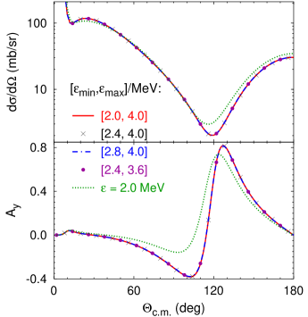
Figure 8: (Color online) Differential cross section and proton analyzing power for elastic $p$-${}^{3}\mathrm{He}$ scattering at 25 MeV proton energy as functions of c.m. scattering angle. Results obtained using different sets of $\varepsilon$ values ranging from $\varepsilon_{\mathrm{min}}$ to $\varepsilon_{\mathrm{max}}$ with the step of 0.4 MeV are compared; they are indistinguishable. The dotted curves refer to the $\varepsilon=2.0$ MeV calculations without extrapolation that have no physical meaning but demonstrate the importance of the extrapolation.

As pointed out in ref. [65], the calculations keeping the same grids but with standard integration weights fail completely at $\varepsilon$ values from Table 1, with the errors of the $\varepsilon\to+0$ extrapolation being up to 10 % for phase shifts and up to 25 % for inelasticity parameters. On the other hand, at large $\varepsilon>4$ MeV the two integration methods agree well but the $\varepsilon\to+0$ extrapolation has at least one order of magnitude larger inaccuracies than those presented in Table 1.

Figure 9: (Color online) Differential cross section for elastic $p\text{-}{}^{3}\mathrm{He}$ scattering at 8.52, 19.4, and 35.0 MeV proton energy as function of the c.m. scattering angle. Results obtained with INOY04 (solid curves), CD Bonn (dashed-dotted curves), and AV18 (dotted curves) potentials are compared with the experimental data from Refs. [135, 136].

An example for the physics results obtained with various realistic high-precision NN potentials, namely, the Argonne (AV18) potential [7], the charge-dependent Bonn potential (CD Bonn) [8], and the INOY04 potential, is presented in Fig. 9. The differential cross section $d\sigma/d\Omega$ for elastic $p\text{-}{}^{3}\mathrm{He}$ scattering at a number of proton energies ranging from $E_{p}=8.5$ to 35.0 MeV is shown. This observable decreases rapidly with the increasing energy and also changes the shape; the calculations describe the energy and angular dependence of the experimental data fairly well. Below $E_{p}=10$ MeV the experimental data are slightly underpredicted at forward angles as happens also at energies below the three-cluster breakup threshold [137, 58]. At the minimum the $d\sigma/d\Omega$ predictions scale with the ${}^{3}\mathrm{He}$ binding energy: the weaker the ${}^{3}\mathrm{He}$ binding the lower the dip of $d\sigma/d\Omega$ that is located between $\Theta_{\mathrm{c\!\>\!.m\!\>\!.}}=105^{\circ}$ and $\Theta_{\mathrm{c\!\>\!.m\!\>\!.}}=125^{\circ}$. The scaling is more pronounced at higher energies. For the INOY04 potential that fits the ${}^{3}\mathrm{He}$ binding energy, one gets excellent agreement in the whole angular region up to $E_{p}\simeq 20$ MeV but, as the energy increases, the calculated cross section starts underpredicting the data. This may be a sign for the need of a three-nucleon force. More detailed study of the elastic $p\text{-}{}^{3}\mathrm{He}$ scattering, including various spin observables like analyzing powers, spin-correlation and spin-transfer coefficients, can be found in ref. [66].

In summary, realistic and fully converged four-nucleon scattering calculations above the four-nucleon breakup threshold becomes feasible using the complex energy method with a special integration technique in the momentum-space framework. The only stumbling block at the present time for momentum-space four-nucleon calculations is adding a state of the art static three-nucleon force to the underlying realistic NN force. However, effective 3N and 4N forces have been included via explicit NN-N$\Delta$ coupling in the two-baryon potential, both below [61] and above [66] breakup threshold. Extension of the method to other reactions in the 4N system is in progress.

7 Momentum lattice technique

The momentum lattice technique developed in Refs. [138, 139, 140, 141] is based on the idea of discretization of all momentum variables using finite wave-packet basis of the so-called $L_{2}$ type. In this respect it has some similarity with the continuum discretized coupled channels (CDCC) method [142]. In contrast to free waves employed in the standard momentum-space scattering calculations, $L_{2}$ basis states are square-integrable functions much like the bound-state wave functions. Thus, in this approach the few-body scattering problem is formulated in a Hilbert space of few-body normalized states, and all involved operators are approximated by finite-dimensional matrices. In this respect it is similar to the bound-state problem. The method has been successfully applied to study neutron-deuteron elastic scattering and breakup using semirealistic as well as realistic interactions [140, 141, 143]. In this section these developments are summarized.

The description of three identical particles uses the standard Jacobi momenta ${\mathbf{p}}$ and ${\mathbf{q}}$ that coincide with ${\mathbf{k}}_{x}$ and ${\mathbf{k}}_{y}$ in eq. (57), respectively. The corresponding continuum partial-wave states are normalized to Dirac $\delta$-functions (note, however, a different convention as compared to previous section) $\langle p^{\prime}|p\rangle=\delta(p^{\prime}-p)$ and $\langle q^{\prime}|q\rangle=\delta(q^{\prime}-q)$ where the dependence on the angular momentum, spin, and isospin quantum numbers is suppressed for simplicity. The continuum part of the momenta $0\leq p\leq p_{\rm max}$ is divided into $M$ nonoverlapping bins $\mathfrak{D}_{i}\equiv[p_{i-1},p_{i}]$ with $i=1,\ldots,M$ whereas the high-momentum part of the spectrum above $p_{\rm max}$ is neglected. In the same manner the continuum part of momenta $0\leq q\leq q_{\rm max}$ is divided into $N$ nonoverlapping bins $\bar{\mathfrak{D}}_{j}\equiv[q_{j-1},q_{j}]$ and the high-momentum part above $q_{\rm max}$ is again neglected. The widths of the momentum bins are $d_{i}=p_{i}-p_{i-1}$ and $\bar{d}_{j}=q_{j}-q_{j-1}$, respectively. The partial-wave packet $L_{2}$ basis is constructed as

$$|\mathfrak{p}_{i}\rangle=\frac{1}{\sqrt{A_{i}}}\int_{\mathfrak{D}_{i}}dpf(p)|p\rangle,\quad i=1,\ldots,M,$$ (66)

$$|\mathfrak{q}_{j}\rangle=\frac{1}{\sqrt{B_{j}}}\int_{\bar{\mathfrak{D}}_{j}}dqw(q)|q\rangle,\quad j=1,\ldots,N.$$ (67)

Here $f(p)$ and $w(q)$ are freely chosen weight functions with the corresponding normalization factors

$$A_{i}=\int_{\mathfrak{D}_{i}}dp|f(p)|^{2},$$ (68)

$$B_{j}=\int_{\bar{\mathfrak{D}}_{j}}dq|w(q)|^{2}$$ (69)

ensuring the desired normalization $\langle\mathfrak{p}_{i^{\prime}}|\mathfrak{p}_{i}\rangle=\delta_{i^{\prime}i}$ and $\langle\mathfrak{q}_{j^{\prime}}|\mathfrak{q}_{j}\rangle=\delta_{j^{\prime}j}$ of the wave packet states. One of the simplest possible choices for the weight functions is $f(p)=1$ resulting in $A_{i}=d_{i}$. In this case the momentum representation of the wave packet

$$\langle p|\mathfrak{p}_{i}\rangle=\frac{\vartheta(p\in\mathfrak{D}_{i})}{\sqrt{d_{i}}},$$ (70)

takes a form of step-like function where $\vartheta(p\in\mathfrak{D}_{i})\equiv\vartheta(p-p_{i-1})\vartheta(p_{i}-p)$.

The three-body wave packet states are built as direct products of the above wave packets for the pair and spectator particle motion, i.e., $|\mathfrak{p}_{i}\rangle\otimes|\mathfrak{q}_{j}\rangle$. Since the basis functions are the products of both step-like functions in variables $p$ and $q$, the solution of the three-body scattering problem in such a basis corresponds to a formulation of the scattering problem on a two-dimensional momentum lattice, with lattice cells $\mathfrak{D}_{ij}=\mathfrak{D}_{i}\otimes\bar{\mathfrak{D}}_{j}$. Using such a lattice basis, in principle one could solve the three-body scattering problem by projecting all the scattering operators onto wave packet states. In this representation the free Hamiltonian $H_{0}$ as well as the free resolvent $G_{0}=(Z-H_{0})^{-1}$ remain diagonal; their matrix elements have explicit analytical forms [138]. Other operators, e.g., the three-body transition operator ${U}_{1}$ of eq. (55), must be transformed into lattice basis according to relations (66) and (67) thereby becoming finite-dimensional matrices

$$[{\mathbb{U}}_{1}]_{i^{\prime}j^{\prime},ij}=\frac{1}{\sqrt{A_{i^{\prime}}B_{j^{\prime}}A_{i}B_{j}}}\int_{\mathfrak{D}_{i^{\prime}j^{\prime}}}dp^{\prime}dq^{\prime}\int_{\mathfrak{D}_{ij}}dpdqf(p^{\prime})w(q^{\prime})\langle p^{\prime}q^{\prime}|U_{1}|pq\rangle f(p)w(q).$$ (71)

As an alternative to the free wave packets discussed so far, one may consider scattering wave packets for the correlated pair of particles constructed as

$$|\psi(\mathfrak{p}_{i})\rangle=\frac{1}{\sqrt{A_{i}}}\int_{\mathfrak{D}_{i}}dpf(p)|\psi(p)\rangle.$$ (72)

Here $|\psi(p)\rangle$ is the exact scattering wave function corresponding to the channel Hamiltonian $H_{1}=H_{0}+v_{1}$ with $v_{1}$ being the potential for the pair 1 consisting of particles 2 and 3 in the odd-man-out notation. Of course, the binning $\mathfrak{D}_{i}$, the weight function $f(p)$, and the respective normalization factors $A_{i}$ can be chosen differently as compared to eq. (66). If the Hamiltonian $H_{1}$ supports also a bound state, the set of scattering wave packets (72) has to be accomplished with this bound state wave function $|\psi_{0}\rangle$ to form an orthonormalized basis. In such basis the channel Hamiltonian $H_{1}$ and the respective channel resolvent $G_{1}=(Z-H_{1})^{-1}$ are diagonal [138]. This suggests an alternative form of three-body scattering equations instead of (55) for the transition operator $U_{1}$. Given the identity $tG_{0}=v_{1}G_{1}$ and that on-shell $(G_{0}^{-1}-v_{1})|\psi_{0}\rangle=0$, the three-body transition operator $\tilde{U}$ satisfying the integral equation

$$\tilde{U}=P_{1}v_{1}+P_{1}v_{1}G_{1}\tilde{U},$$ (73)

is equivalent to $U_{1}$ on- and half-shell and therefore describes the same scattering process. An essential advantage of this approach is that the singularities are integrated out when calculating the matrix elements of the operators in eq. (73) in the momentum-lattice basis such that the resulting matrix equations are nonsingular. Furthermore, explicit calculation of the two particle transition matrix $t$ and its interpolations are avoided.

In practical calculations the knowledge of the exact scattering wave packets (72) is not necessary since they are approximated by the pseudostates $|\tilde{\psi}(\mathfrak{p}_{i})\rangle$ obtained by the diagonalization of the channel Hamiltonian $H_{1}$ in the basis of free wave packets (66), i.e.,

$$|\tilde{\psi}(\mathfrak{p}_{k})\rangle=\sum_{i=1}^{M}O_{ki}|\mathfrak{p}_{i}\rangle,\quad k=1,\ldots,M,$$ (74)

with $O_{ki}$ being the elements of the respective transformation matrix. It has been demonstrated in ref. [138] that the properties of $|{\psi}(\mathfrak{p}_{i})\rangle$ and $|\tilde{\psi}(\mathfrak{p}_{i})\rangle$ are quite similar thereby justifying the above approximation. To solve the scattering equations in the pseudostate basis (74) the corresponding transformations for the matrices of all involved operators has to be done. Finally, since the basis states are step-like functions of momenta and/or energies, the energy-averaging procedure has to be applied to obtain the breakup amplitudes from the solutions of the finite-dimensional matrix equations for $\tilde{\mathbb{U}}$, as described in detail in ref. [141].

The above momentum lattice method has been first tested in a model study of neutron-deuteron elastic scattering and breakup with semirealistic interactions limited to $S$ waves [140, 141]. More recently the results for elastic neutron-deuteron scattering were obtained also with realistic interactions [143]. The method was able to reproduce reasonably well the results obtained in standard momentum-space calculations, but, in its presently available technical implementation [143] is still less efficient than the standard momentum-space methods of refs. [1, 3]. Thus, it remains yet unclear if the momentum lattice method could be extended beyond the A=3 case in realistic few-body scattering calculations. On the other hand, the momentum lattice method has additional advantages when performing calculations at several energies simultaneously, and in systems with charged particles where one could use Coulomb wave packets thereby avoiding screening and renormalization procedure. Due to the finite $L_{2}$ character of the wave packet basis which is rather similar to the harmonic oscillator basis one can use the Hamiltonian diagonalisation procedure to find the scattering states and the S-matrix, thereby avoiding the need for the solution of scattering equations at all [144]. Finally, the momentum lattice method is better suited for implementing the calculations on graphic processor units, leading to significant gains in speed [143].

We would like to mention the existence of other techniques to compute scattering observables which are also based on bound state solutions in a discretized space, although in a quite a different spirit of what has been presented above. They were developed by Luscher and collaborators [145] in a series of papers devoted to Lattice QCD [146]. These techniques are based on computing the volume dependence of the confined solutions and obtaining from them the corresponding low energy scattering parameters. First formulated in the framework of non relativistic quantum mechanics, they were aimed to extract the scattering observables from the solution of a Quantum Field theoretical problem obtained using the Feynman path integral formulation of the theory in an euclidean discretized space-time with periodic and/or anti-periodic boundary conditions. They overcome this way the no-go theorem of Maiani and Testa [147], damming the access to the scattering observables from any euclidean discretized version of a Quantum Field theory in a finite volume. The present applications of this technique are however limited to the scattering of simple two-body composite systems, far from the complexity of the asymptotic many-body multichannel wavefunctions, esspecially in presence of the breakup channels. The interested reader can take benefit in consulting the recent reviews on this topic in different fields of application [148, 149].

8 Summary and Outlook

The last two decades have witnessed a real revolution in the ab initio treatment of the nuclear bound state problem based on nonrelativistic Hamiltonians. Important steps have been taken in improving our understanding of the interaction between nucleons, including two- and three-nucleon forces [150, 151]. Moreover, ab initio bound state methods that allow a solution of the nuclear many-body problem without any uncontrolled approximation have been evolved to treat systems with dozens of nucleons [152, 69, 153, 68].

The ab initio treatment of nuclear collision problems has instead progressed at a modest pace. Nevertheless, key steps have been also undertaken in this direction. The first serious issue is related with the inclusion of the Coulomb interaction for the collision above the three-cluster breakup threshold. This problem has been overcome both by momentum space as well as coordinate space methods, using very different techniques [2, 15, 16, 41, 43]. The next important step was to demonstrate the possibility of exact solutions of multiparticle problems in $A>3$ systems above breakup threshold. This has been also achieved almost simultaneously by the developments in momentum and coordinate space frameworks [64, 65, 42].

The next important challenge is to push forward calculations of collision problems to the level achieved by the modern bound state methods, i.e. well beyond the $A=4$ system. This challenge is well understood by the leading developers of bound-state methods who started switching gears to the problem of nuclear collisions. Yet, up to this moment, most developments involve approximate prescriptions of the scattering problem [70, 154, 68]. The main difficulty of the collision problem is related to the complex asymptotic form of the wave function in coordinate space, which gives rise to a complex structure of singularities when describing multiparticle dynamics using integral equations in momentum space. Furthermore, the complexity of the wave function asymptotic form (integral kernel singularities) quickly rises once multiparticle breakup channels become open. Therefore the importance of exact methods enabling to the treatment of the multiparticle scattering problem by avoiding these formal as well as technical difficulties is well understood and turns out to be crucial for further developments.

The goal of this review is to demonstrate available tools to solve the scattering problem exactly. We have overviewed five different methods, namely: Lorentz Integral Transform, Continuum discretization, Complex Scaling, Complex energy, and Momentum lattice methods. All of these methods are able to handle multiparticle scattering problems rigorously, both below and above breakup threshold and provide full information about the respective integral as well as differential observables.

The Lorentz Integral Transform method remains limited to the breakup of bound systems by an external perturbation; however this method has been already implemented beyond the $A=4$ system and seems to be the most easy to incorporate in many-body calculations [67].

The Continuum discretization method formally requires no modifications in the existing bound state techniques to be implemented to treat the scattering problem. One should only be able to adjust the calculated positive energy eigenvalues to the energy of the collision. Difficulties in implementing this method may however appear for systems with multiple binary channels. One should find as many independent solutions as there are channels, which may turn out into a complex technical task.

The last difficulty is not present in the Complex Scaling or Complex Energy methods. Implementation of these method is also rather straightforward with any bound state method, once one extends the available codes to handle complex arithmetics. This may require not only simple modification of the arithmetical operations used in the computer codes but also adjustment of the linear algebra routines, which sometimes are only proper for real Hermitian matrices. Nevertheless, very efficient iterative linear algebra methods have been developed by the mathematicians and software developers during the last decade [155], that may handle algebraic problems for general complex matrices. An efficient implementation of the Complex Energy method requires, however, special numerical techniques beyond the standard bound state calculations.

Still one important step should be undertaken to handle these methods in conjunction with the most-advanced bound state codes. Solution of the scattering problem as well as calculation of the observables requires construction of the incoming wave function. This wave function is based on bound-state wave functions of inherent clusters, and thus formally should be available. Nevertheless composed cluster wave functions should be fully consistent with the full Hamiltonian. This last issue may in fact be an important handicap for some methods, since optimal variational parameters used to calculate the N-body system may differ from the ones applied in composed cluster calculations present in the incoming wave. Likewise some similarity transformations used to make strong the interaction easier to treat by bound state methods, like Lee-Suzuki transform [156], are particle number dependent and thus may not be appropriate for the scattering problem. Nevertheless the similarity renormalization group interactions which do not depend on the particle number are beeing actively developed and have become very popular in bound-state calculations.

We believe that the next decade will be crucial for further evolution in the many-body scattering problem. Moreover, experimental installations of the next generation, based on radioactive ion beams, are becoming available in the near future. These experiments require a quantitatively better understanding and interpretation of the nuclear collision process [157, 158, 159] given the unstable nature of the projectiles. The recent developments we present in this manuscript may provide the necessary tools to overcome serious difficulties in the solution of the multiparticle scattering problem.

Acknowledgments

The authors thank G. Orlandini, V. N. Pomerantsev and V. I. Kukulin for discussions and details of their calculations.

References

- [1] W. Glöckle, H. Witała, D. Hüber, H. Kamada, J. Golak, The three-nucleon continuum: Achievements, challenges and applications, Phys. Rep. 274 (1996) 107.
- [2] A. Kievsky, M. Viviani, S. Rosati, Phys. Rev. C 64 (2001) 024002.
- [3] A. Deltuva, K. Chmielewski, P. U. Sauer, Phys. Rev. C 67 (2003) 034001.
- [4] L. D. Faddeev, Zh. Eksp. Teor. Fiz. 39 (1960) 1459, [Sov. Phys. JETP 12, 1014 (1961)].
- [5] E. O. Alt, P. Grassberger, W. Sandhas, Nucl. Phys. B2 (1967) 167.
- [6] V. G. J. Stoks, R. A. M. Klomp, C. P. F. Terheggen, J. J. de Swart, Nijmegen, Phys. Rev. C 49 (1994) 2950.
- [7] R. B. Wiringa, V. G. J. Stoks, R. Schiavilla, Av18, Phys. Rev. C 51 (1995) 38.
- [8] R. Machleidt, High-precision, charge-dependent bonn nucleon-nucleon potential, Phys. Rev. C 63 (2001) 024001.
- [9] E. Epelbaum, W. Glöckle, U.-G. Meissner, Nucl. Phys. A671 (2000) 295.
- [10] D. R. Entem, R. Machleidt, Accurate charge-dependent nucleon-nucleon potential at fourth order of chiral perturbation theory, Phys. Rev. C 68 (2003) 041001(R).
- [11] R. Machleidt, D. R. Entem, Chiral effective field theory and nuclear forces, Phys. Rep. 503 (2011) 1.
- [12] H. Witała, T. Cornelius, W. Glöckle, Elastic scattering and break-up processes in the n-d system, Few-Body Systems 3 (1988) 123.
- [13] H. Witała, T. Cornelius, W. Glöckle, Faddeev calculations with meson exchange interactions for the break-up process, Few-Body Systems 5 (1988) 89.
- [14] J. L. Friar, B. F. Gibson, G. Berthold, W. Glöckle, T. Cornelius, H. Witala, J. Haidenbauer, Y. Koike, G. L. Payne, J. A. Tjon, W. M. Kloet, Benchmark solutions for a model three-nucleon scattering problem, Phys. Rev. C 42 (5) (1990) 1838–1840. doi:10.1103/PhysRevC.42.1838.
- [15] A. Deltuva, A. C. Fonseca, P. U. Sauer, Phys. Rev. C 71 (2005) 054005.
- [16] A. Deltuva, A. C. Fonseca, P. U. Sauer, Phys. Rev. C 72 (2005) 054004.
-
[17]
C. R. Chen, G. L. Payne, J. L. Friar, B. F. Gibson,
Low-energy
nucleon-deuteron scattering, Phys. Rev. C 39 (1989) 1261–1268.
doi:10.1103/PhysRevC.39.1261.
URL http://link.aps.org/doi/10.1103/PhysRevC.39.1261 - [18] J. L. Friar, G. L. Payne, W. Glöckle, D. Hüber, H. Witała, Benchmark solutions for n-d breakup amplitudes, Phys. Rev. C 51 (5) (1995) 2356–2359. doi:10.1103/PhysRevC.51.2356.
- [19] A. Kievsky, J. L. Friar, G. L. Payne, S. Rosati, M. Viviani, Phys. Rev. C 63 (2001) 064004.
- [20] A. Deltuva, A. C. Fonseca, A. Kievsky, S. Rosati, P. U. Sauer, M. Viviani, Phys. Rev. C 71 (2005) 064003.
-
[21]
E. P. Wigner, Resonance
reactions and anomalous scattering, Phys. Rev. 70 (1946) 15–33.
doi:10.1103/PhysRev.70.15.
URL http://link.aps.org/doi/10.1103/PhysRev.70.15 -
[22]
E. P. Wigner, Resonance
reactions, Phys. Rev. 70 (1946) 606–618.
doi:10.1103/PhysRev.70.606.
URL http://link.aps.org/doi/10.1103/PhysRev.70.606 -
[23]
E. P. Wigner, L. Eisenbud,
Higher angular momenta
and long range interaction in resonance reactions, Phys. Rev. 72 (1947)
29–41.
doi:10.1103/PhysRev.72.29.
URL http://link.aps.org/doi/10.1103/PhysRev.72.29 - [24] P. Descouvemont, D. Baye, The R-matrix theory, REPORTS ON PROGRESS IN PHYSICS 73 (3). doi:10.1088/0034-4885/73/3/036301.
- [25] P. Descouvemont, E. Tursunov, D. Baye, Three-body continuum states on a Lagrange mesh, NUCLEAR PHYSICS A 765 (3-4) (2006) 370–389. doi:10.1016/j.nuclphysa.2005.11.010.
- [26] K. Arai, S. Aoyama, Y. Suzuki, P. Descouvemont, D. Baye, Tensor Force Manifestations in Ab Initio Study of the H-2(d, gamma)He-4, H-2(d, p)H-3, and H-2(d, n)He-3 Reactions, PHYSICAL REVIEW LETTERS 107 (13). doi:10.1103/PhysRevLett.107.132502.
-
[27]
V. D. Efros, W. Leidemann, G. Orlandini,
Response
functions from integral transforms with a lorentz kernel, Physics Letters B
338 (23) (1994) 130 – 133.
doi:10.1016/0370-2693(94)91355-2.
URL http://www.sciencedirect.com/science/article/pii/0370269394913552 - [28] A. La Piana, W. Leidemann, Calculation of exclusive cross sections with the Lorentz integral transform method, NUCLEAR PHYSICS A 677 (2000) 423–441.
-
[29]
J. Golak, R. Skibiński, W. Glöckle, H. Kamada, A. Nogga, H. Witała,
V. Efros, W. Leidemann, G. Orlandini, E. Tomusiak,
Benchmark
calculation of the three-nucleon photodisintegration, Nuclear Physics A
707 (34) (2002) 365 – 378.
doi:10.1016/S0375-9474(02)00989-2.
URL http://www.sciencedirect.com/science/article/pii/S0375947402009892 -
[30]
S. Quaglioni, W. Leidemann, G. Orlandini, N. Barnea, V. D. Efros,