Singularity formation for Prandtl’s equations

Abstract

We consider Prandtl’s equations for the impulsively started disk and follow the process of the formation of the singularity in the complex plane using the singularity tracking method. We classify Van Dommelen and Shen’s singularity as a cubic root singularity.

We introduce a class of initial data which have a dipole singularity in the complex plane. These data are uniformly bounded in $H^{1}$ and lead to an earlier singularity formation. The presence of a small viscosity in the streamwise direction changes the behavior of the singularities.

1 Introduction

The aim of this paper is to perform a numerical study of the process of singularity formation for the solutions of Prandtl’s equations. The main reason that motivates this study is that the mathematical theory of Prandtl’s equations is still unclear, as no well posedness result, under general hypotheses on the data, is available. It would be an advance in the mathematical theory of fluid dynamics to prove that the solutions of Prandtl’s equations remain (for a short time) regular when the initial and boundary data have (for example) a Sobolev type of regularity; or to disprove this, constructing a class of data, bounded in a Sobolev space, for which a zero time blow-up of the solutions occurs.

The main result of this paper is a numerical evidence of the ill-posedness of Prandtl’s equations in $H^{1}$. Other results we shall obtain with our investigation are the following. First the blow-up of Prandtl’s solution for the impulsively started disk will be shown to be the consequence of a complex singularity, of cubic-root type, hitting the real $x$ axis; this result had already been found in [16], but in this paper we give further evidences also using more refined numerical schemes. Second we shall see that this structure of the singularity is robust with respect to perturbations (belonging to a class we shall specify later) of the initial datum as well of the matching datum. Third the blow-up time for the solution will be shown to be related to the $\sup$ of the derivative of the initial datum, at least when the complex singularity is relatively close to the real axis. Finally the presence of a small viscosity in the streamwise direction is able to prevent the formation of the singularity (a result already present in [16]), while the number of Fourier modes effectively excited tends to be linearly dependent on the streamwise viscosity.

In the rest of this Introduction we shall briefly recall what the Van Dommelen and Shen singularity is, and give a short account on the mathematical theory of Prandtl’s equations. For more details on these topics we shall refer the reader to the review papers available in the literature.

1.1 Separation and singularity in the boundary layer

Boundary layer separation is the most striking phenomenon that one encounters considering the interaction of a slightly viscous (or, said differently, with high Reynolds number) flow with a solid boundary. Unsteady separation has been puzzling the researchers for many decades. The importance of this phenomenon stays in the fact that separation is the mechanism through which the vorticity generated at the boundary is ejected into the outer flow and it is therefore considered as one of the responsible of the transition to turbulence in wall bounded fluids.

In this contest the case of the 2D flow past an impulsively started disk has attracted great interest because it served as a case study where (since the early stages of the investigations) the appearance of reverse flow, recirculation, separation, vorticity shedding were proposed as a possible universal route to the onset of turbulence. The seminal work of Van Dommelen and Shen [41, 42] (see also e.g. [40]) clarified how separation is linked to the appearance of a singularity in the solution of Prandtl’s equations. In their Lagrangian framework the singularity appeared as a fluid particle being squashed in the streamwise direction to zero thickness, therefore causing (in absence of normal pressure gradients, as it is the case for Prandtl’s equations) an eruption in the normal direction. Subsequent calculations by different authors both in Lagrangian coordinates as well using finite difference or spectral [24] methods in Eulerian coordinates confirmed the results of Van Dommelen and Shen, and the fact that Prandtl’s equations develop singularity became an accepted statement in the literature.

More problematic is the relationship between the process of separation for the high Reynolds number Navier-Stokes flow and the singularity of Prandtl’s solution. Although the qualitative picture of the Navier-Stokes solutions, with the appearance of high gradients in the streamwise velocity, resembles the structure of the singularity in Prandtl’s solution, a more careful quantitative study reveals that the interaction of the boundary layer flow with the outer flow sets in well before the singularity time for Prandtl’s equations (see [13]), at least for the Reynolds numbers that have been tested so far, which are about $10^{7}$.

It is almost impossible here to review the relevant literature regarding the development of the boundary layer theory after Van Dommelen and Shen’s breakthrough, and we refer the interested reader to [14].

1.2 The mathematical theory of Prandtl’s equations

The fact that the appearance of a singularity seems related to a physical phenomenon (separation) that experimentalists have observed for decades makes the mathematical theory of Prandtl’s equations relevant also from the applied point of view. Moreover the well- or the ill-posedness of Prandtl’s equations is related to a fundamental question of theoretical fluid dynamics, i.e. the convergence of the Navier–Stokes solutions to the solutions of the Euler equations away from boundaries. The first results on the existence and the uniqueness issue for the solutions of Prandtl’s equations were obtained by Oleinik and her coworkers (see e.g. [29]). Basically Oleinik’s theory (which is reviewed in great detail in [30]) deals with monotonous data, in the sense that e.g. $\partial_{y}u_{0}>0$, $u_{0}$ being the initial datum. In this case Oleinik and her coworkers were able to get short time existence of regular solutions (or long time existence for small domains). Recently, adding the hypothesis of a favorable pressure gradient (i.e. $\partial_{x}p\leq 0$), Xin and Zhang in [43] proved the long time existence of weak solutions. Other results, concern the case of analytic data. In [34] (see also [2]), the authors proved the short time existence and uniqueness when the data are analytic; this result was improved in [10, 26] where it is required analyticity in the streamwise direction while, using the regularizing effect of the viscosity, only $C^{2}$ regularity in the normal direction is found to be necessary. On the other side there is the result of E and Engquist [18] which for a flat boundary proved that, if the initial data is of the form $u_{0}=-xb_{0}(x,y)$, and if $\partial_{x}u_{0}(x=0,y)$ satisfies a technical assumption, then at $x=0$ the solution terminates in a blow up of the tangential derivative. For a review on the mathematical theory of Prandtl’s equations, see [9, 17] and also [5].

Regarding the related problem of the convergence of Navier–Stokes solutions in the zero viscosity limit, we mention the result in [35] where for analytic data the authors prove convergence to Euler and Prandtl’s solutions (away and close to the boundary respectively), and the criteria of Kato [25] and of Temam and Wang [38]. Assuming an a priori estimate on the solution close to the boundary, (on the energy dissipation in [25] or on the pressure gradient in [38]), one gets convergence to the Euler solution away from the boundary.

On the other hand Grenier, in [21], proved that there are initial profiles (those profiles for which Euler equations are linearly unstable) for which the exponential growth of modes of size $\mbox{Re}^{1/2}$ (i.e. a phenomenon linked to Rayleigh instability) does not allow the solution to have the form of a matched asymptotic expansion between a Prandtl solution and an Euler solution. The findings of Brinckman and Walker are probably somehow related to this result. In [7], using the full 3D Navier–Stokes equations, they studied the response of the boundary layer to an array of counter-rotating vortices placed in the outer flow. Their goal was to mimic the mechanism through which vorticity regenerates in the boundary layer. They found that the time at which the Rayleigh instability caused rapidly growing oscillations inside the boundary layer was shorter than the time at which Van Dommelen and Shen’s singularity developed which posed again the question whether (or up to what time) the Navier–Stokes solutions are correctly described by Prandtl’s equations. Although more recent (at higher resolution) calculations [28] seem to cast some doubt on the prediction of [7] of an early development of instabilities, Brinckman and Walker pose an important problem, see the discussion in [14] where the possibility of the Rayleigh instabilities winning the race with Van Dommelen and Shen’s singularity is suggested also for data with exponentially decaying spectra (i.e. analytic data).

1.3 Plan of the paper

In this paper we investigate, mostly in the case study of the $2D$ impulsively started disk, the process of the singularity formation for Prandtl’s equations using the singularity tracking technique. This methodology was initiated in [37], and is based on the idea that the blow-up of the solution (or of its derivative) of a PDE is preceded by the appearance, in the plane of the complexified spatial variable, of a complex singularity. The real blow-up is the consequence of the singularity hitting the real axis. The location of the complex variable can be determined studying the asymptotic behavior of the Fourier spectrum. Although the method was originally introduced to investigate the possibility of the finite time blow up of the $3D$ Euler solutions (see e.g. [8, 19, 27, 32]), it turned out to be a powerful tool to characterize the process of singularity formation for many PDEs, see for example [15, 20, 33, 36].

In Section 2 we describe all the various numerical method we used to solve Prandtl’s equations in the case of the 2D impulsively started disk. They are all spectral method in the streamwise direction while in the normal direction we have used both finite-differences and spectral methods (using Chebychev polynomials). For the discretization in time various methods have been used. All these numerical procedures lead to the same conclusions, and this gives some reliability to our results. In this Section we shall also describe the singularity tracking method, both in $1D$ and in $2D$.

In Section 3 we study the Van Dommelen and Shen singularity.

In Section 4 we propose to study Prandtl’s equations imposing a class of real analytic (with respect to the streamwise direction while it is $C^{2}$ w.r.t. the normal variable) initial data that have an algebraic singularity placed at some distance $\delta_{0}$ from the real axis. To be more precise we take Van Dommelen and Shen’s solution at time $t=1.5$ (when their singularity is quite far away from the real axis: we recall that the VDS singularity time is $t\approx 3$) and add a singularity placed at distance $\delta_{0}$ from the real axis. The spectrum of our data behaves like $|k|^{-5/3}$. This means that, however small $\delta_{0}$ is, all the data in this class have $H^{1}$ norm bounded by some constant. Moreover the singularity we are placing in the complex plane can be thought of as a couple of singularities of opposite sign infinitely close and infinitely strong. We call this singularity “dipole singularity”. In Section 4 we show that this singularity travels toward the real axis to lead to a blow up of the solution in a time shorter than the typical Van Dommelen and Shen’s singularity time.

In Section 5 we study how Burger’s equation develops singularity for the dipole singularity initial data. We see how, in the well understood case of Burger’s equation (in fact one knows the relationship between the singularity time and the $\sup$ norm of the derivative of the initial datum), one can make arbitrarily short the singularity time picking the $\delta_{0}$ sufficiently small.

In Section 6 we see that the situation seems to be the same for Prandtl’s equation.

In Section 7 we propose to study Prandtl’s equations with the presence of the regularizing viscosity in the streamwise direction. We will see that a small viscosity in $x$ is able to prevent the singularity formation. The singularity, still headed to the real axis, fails to reach it and stabilizes at a distance that depends on the amount of viscosity in $x$. In this section we also clarify how the class of initial data introduced in Section 4 has the physical meaning of a couple of counter–rotating vortices placed inside the boundary layer.

2 The equations and the numerical methods

In this section first we shall introduce Prandtl’s equations in the case of an impulsively started disk in a uniform background flow. Second we shall discuss the various numerical methods we have used to solve the equations. Finally we shall give a brief review of the ideas behind the singularity tracking method.

2.1 The equations

Prandtl’s equations describe the behavior of a fluid close to a physical boundary in the zero viscosity limit. These equations can be obtained as a formal asymptotic limit of the Navier–Stokes equations assuming that close to the boundary there is a rapid adjustment between the outer inviscid flow and the inner viscous flow. If in the Navier-Stokes equations one rescales the variable normal to the boundary as $Y=y/\sqrt{\nu}$, to the first order in $\sqrt{\nu}$ one gets the Prandtl equations. In the case of a disk impulsively started in a uniform background flow $U=\sin{(x)}$, Prandtl’s equations are:

$$\partial_{t}u+u\partial_{x}u+v\partial_{Y}u-U\partial_{x}U = \partial_{YY}u\qquad U=\sin{(x)}$$ (2.1)

$$\partial_{x}u+\partial_{Y}v = 0$$ (2.2)

$$u(x,0,t)=v(x,0,t) = 0$$ (2.3)

$$u(x,\infty,0) = U$$ (2.4)

$$u(x,y,0) = U\,.$$ (2.5)

The above equations have to be solved for $(x,Y)\in[0,2\pi]\times[0,\infty[$ for the variable $u$. In fact, the incompressibility condition (2.2) allows to recover the rescaled normal velocity $v$ through an integration in the normal variable. Equation (2.3) and Eq.(2.4) give the boundary condition and the matching condition with the outer flow, while (2.5) is the initial condition.

2.2 The numerical methods I: mixed spectral-finite difference

We solve the above equations in the computational domain $[0,2\pi]\times[0,\overline{Y}]$. One has to choose $\overline{Y}$ big enough so that the solution $u(x,\overline{Y},t)$ has matched exponentially the matching condition (2.4) (i.e. $u(x,\overline{Y},t)-U$ must be small). In our calculations we have chosen $\overline{Y}=20$, as in [22, 23] or [16], which is sufficient to ensure the matching between $u$ and $U$.

To solve the equations in [0,T] one can use a spectral method for the variable $x$ and finite differences for the variable $Y$. Namely, denoting with $\Delta Y=20/(M+1)$ and with $\Delta t=T/N$, we approximate the solution as:

$$u(x,j\Delta Y,n\Delta t)\approx\sum_{k=-K/2}^{K/2}u^{n}_{k,j}e^{ikx}$$

The diffusion term $\partial_{YY}u$ has been treated using the usual three points rule. We have now to specify the way we have discretized the time derivative $\partial_{t}u$, and the nonlinear terms $\partial_{x}F(u)$ and $\partial_{Y}G(u)$ where $F(u)\equiv u^{2}$ and $G(u)\equiv uv$. Regarding the nonlinear term involving the $x$ derivative we have always used the usual pseudo-spectral approximation involving multiplication in the physical space via an inverse FFT, and using the usual $3/2$–rule to handle aliasing effects [11]. As far as the other terms are concerned we have used several algorithms. A possibility is to use the one step Euler method for the time derivative, the Crank–Nicolson method for the diffusion term and to use a Lax-Wendroff approximation for the nonlinear term involving the $Y$ derivative in the form:

$$\begin{array}[]{rcl}[\partial_{Y}G(u)]^{n}_{k,j}&=&\lambda\left([G(u)]^{n}_{k,j-1/2}-[G(u)]^{n}_{k,j+1/2}\right)\qquad\lambda\equiv\Delta t/\Delta Y\,,\\ \left[G(u)\right]^{n}_{k,j+\frac{1}{2}}&=&\frac{1}{2}\left\{v^{n}_{j+\frac{1}{2}}*\left[u^{n}_{j}+u^{n}_{j+1}-\lambda v^{n}_{j+\frac{1}{2}}*\left(u^{n}_{j+1}-u^{n}_{j}\right)\right]\right\}_{k}\,,\\ v^{n}_{k,j+\frac{1}{2}}&=&\frac{1}{2}(v^{n}_{k,j}+v^{n}_{k,j+1})\,,\end{array}$$ (2.6)

where by $*$ we have denoted the (pseudo)-spectral multiplication. The scheme just described, which is the spectral (in $x$) version of the scheme used in [22, 23], has been used in [16] where the convergence properties are described. An improvement on the above scheme is obtained using the implicit–explicit midpoint method $(1,2,2)$ (see [3] for the details) based on the following pair of implicit (for the diffusion term) and explicit (for the nonlinear terms) Runge–Kutta schemes:

0 0 0

1/2 0 1/2

0 1

         

0 0 0

1/2 1/2 0

0 1

(2.7)

The convergence properties of this scheme at various times (well before the singularity time, just before the singularity time and at the singularity time) are given in Table 2.1. Similar results are obtained with the use of higher order IMEX schemes. Notice that in the convergence tables we are reporting the $L^{2}$ and $L^{1}$ errors have been computed up to the area of the computational domain, i.e. as:

$$\|f\|^{2}_{L^{2}}\equiv\sum_{k,j}|f_{k,j}|^{2}\qquad\|f\|_{L^{1}}\equiv\sum_{k,j}|f_{k,j}|\;.$$

To get the real $L^{2}$ and $L^{1}$ norms one should consider the factors $A^{1/2}$ and $A$ with $A\approx 125.6$.

Table 2.1: Convergence of the numerical scheme based on the Lax–Wendroff approximation of $\partial_{Y}G(u)$ and on the IMEX scheme (2.7). We have obtained similar results coupling the Lax–Wendroff approximation with the IMEX scheme (3,4,3) described in [3] pp.158–159.

Grid	$T=1.54$			$T=2.85$			$T=2.97$
($N\times K\times M$)	$L^{2}$	$L^{1}$	$L^{\infty}$	$L^{2}$	$L^{1}$	$L^{\infty}$	$L^{2}$	$L^{1}$	$L^{\infty}$
$10^{4}\times 32\times 127$	$2.5\cdot 10^{-4}$	$1.5\cdot 10^{-4}$	0.001	0.06	0.04	0.207	0.09	0.06	0.345
$2\cdot 10^{4}\times 64\times 255$	$6.3\cdot 10^{-5}$	$3.7\cdot 10^{-5}$	$2.5\cdot 10^{-4}$	0.029	0.018	0.158	0.057	0.039	0.347
$4\cdot 10^{4}\times 128\times 511$	$1.6\cdot 10^{-5}$	$9.5\cdot 10^{-6}$	$6.6\cdot 10^{-5}$	0.012	0.006	0.113	0.037	0.023	0.353

We have also used the Runge–Kutta scheme (3,4,3) given in [3] obtaining similar results. This scheme has the advantage of allowing to take a larger time step size, due to its stability properties.

All these methods give consistent results with each other. In Fig. 4 we report the solution of Prandtl’s equation with initial datum given by (2.5) computed with the IMEX scheme $(1,2,2)$ of (2.7), with $K=1024$ and $M=1023$. All the computations are in agreement with Van Dommelen and Shen’s (VDS) results [41].

2.3 The numerical methods II: fully spectral

We consider the same computational domain $[0,2\pi]\times[0,\overline{Y}]$ with $\overline{Y}=20$ but we use the Chebychev spectral approximation in the normal variable $Y$. To accomplish this, first we use the linear change of variable $Y\rightarrow w$ given by $Y=(w\overline{Y}+\overline{Y})/2$ so that the computational domain becomes $[0,2\pi]\times[-1,1]$. Second we use the fully spectral approximation:

$$u(x,w,t)\thickapprox\sum\limits_{k=-K/2}^{k=K/2}\sum\limits_{j=0}^{j=M}u_{kj}(t)e^{ikx}T_{j}(w)\;,$$ (2.8)

where $T_{j}$ are the Chebychev polynomials of the first kind. Finally, introducing the variable $\zeta$ defined as $w=\cos{(\zeta)}$, we write the above expression as:

$$u(x,\zeta,t)\thickapprox\sum\limits_{k=-K/2}^{k=K/2}\sum\limits_{j=0}^{j=M}u_{kj}(t)e^{ikx}\cos{(j\zeta)}\;,$$ (2.9)

which, inserted in Prandtl’s equation, through the usual $\tau$–method [6, 11], gives a fully spectral approximation scheme. The boundary condition are implemented through the equations:

$$\sum\limits_{j=0}^{M}(-1)^{j}u_{kj}=0,\qquad\sum\limits_{j=0}^{M}u_{kj}=U_{k},\qquad k=-K/2\dots K/2,$$ (2.10)

where $U_{k}$ are the Fourier components of the matching datum $U(x)$ defined in (2.1).

The non-linear terms $F(u)=u^{2}$ and $G(u)=uv$ are calculated by the usual pseudo-spectral approximation and the aliasing effects are handled by the $3/2$–rule.

Discretization in time is done treating explicitly the convective terms and treating diffusion by the Crank-Nicolson approximation. In particular we have used a semi-implicit Runge-Kutta scheme, the two stage RK2/CN, see [6]. We have also tried the three-stage semi-implicit Runge-Kutta scheme RK3/CN and the semi-implicit Adams-Bashforth schemes of second and third order but, as explained in [6], we have noticed that the second-order RK2/CN is more stable as it allows to take bigger time steps.

2.4 Singularity tracking

If an analytic function $u(z)$ has an algebraic singularity at the complex location $z^{*}=x^{*}+i\delta$, and if at the singularity the behavior is $u(z)\approx(z-z^{*})^{\alpha}$, then the Fourier spectrum of $u(z)$ has the following asymptotic behavior [12]:

$$u_{k}\sim|k|^{-(1+\alpha)}\exp{(-\delta|k|)}\exp{(ix^{*}k)}$$ (2.11)

Therefore if one estimates the rate $\delta$ of the exponential decay of the spectrum one gets the distance of the complex singularity from the real axis; the estimate of the period of the oscillations of the spectrum gives the real location $x^{*}$ of the singularity. Resolving the rate of algebraic decay $1+\alpha$, one can classify the singularity type. In particular, when one deals with a PDE with solution $u(t)$, one can detect, with a good degree of reliability, the time at which the singularity develops as given by the first $t_{c}$ at which $\delta(t_{c})=0$.

It is possible to extend the above technique to bi-variate functions, and we refer to [27, 32] for more details. Let $u(x_{1},x_{2})$ a function with Fourier expansion:

$$u(x_{1},x_{2})=\sum_{k_{1},k_{2}}u_{k_{1}k_{2}}e^{ik_{1}x_{1}}e^{ik_{2}x_{2}}\;.$$

If in the Fourier $\mathbf{k}$–space one considers those modes $(k_{1},k_{2})$ such that $k_{1}=k\cos{(\theta)}$, $k_{2}=k\sin{(\theta)}$ where $k=|(k_{1},k_{2})|$, then the Fourier coefficients, when $k\rightarrow\infty$, have the following asymptotic behavior:

$$u_{k_{1}k_{2}}\approx k^{-\left(\alpha(\theta)+1\right)}e^{-\delta(\theta)k}e^{ikx^{*}(\theta)}\qquad(k_{1},k_{2})=k(\cos{(\theta)},\sin{(\theta)})\;.$$ (2.12)

The width of the analyticity strip $\overline{\delta}$ is the minimum over all directions $\theta$, i.e. $\delta^{*}=\min_{\theta}\delta(\theta)$.

A second way to extend the singularity tracking method to bi-variate functions is to define the shell-summed Fourier amplitudes:

$$A_{K}\equiv\sum_{K\leq|(k_{1},k_{2})|<K+1}\left|u_{k_{1}k_{2}}\right|\;,$$

which is a kind of discrete angle average of the Fourier coefficients. The asymptotic behavior of these amplitudes is:

$$A_{K}\approx CK^{-\left(\alpha_{Sh}+1/2\right)}\exp{\left(-\delta_{Sh}K\right)}\qquad\mbox{when}\quad K\rightarrow\infty\;,$$

where $\delta_{Sh}$ gives the width of the analyticity strip while the algebraic prefactor $\alpha_{Sh}$ gives informations on the nature of the singularity.

As pointed out in [32], using a steepest descent argument, one can see that the two techniques are equivalent. In fact, if one denotes with $\theta^{*}$ the angle where $\delta(\theta)$ takes its minimum (i.e. $\delta^{*}=\delta(\theta^{*})$), one has that $\delta_{Sh}=\delta(\theta^{*})$ and that $\alpha_{Sh}=\alpha(\theta^{*})-1/2$.

An interesting situation is when the most singular direction coincides with one of the coordinate axes, e.g. $\theta^{*}=0$. In this case it is easy to see that, to evaluate the width of the strip of analyticity, one can consider the variable $x_{2}$ as a parameter and adopt the following procedure. First take the Fourier expansion relative to the variable $x_{1}$:

$$u(x_{1},x_{2})=\sum_{k_{1}}u_{k_{1}}(x_{2})e^{-ik_{1}x_{1}}\,;$$

second use that the spectrum has the asymptotic behavior:

$$u_{k_{1}}(x_{2})\approx k_{1}^{-(\alpha(x_{2})+1)}e^{-\tilde{\delta}(x_{2})k_{1}}\;$$

finally get the width of analyticity as the minimum of $\tilde{\delta}(x_{2})$, i.e.:

$$\delta_{Sh}=\min_{x_{2}}\tilde{\delta}(x_{2}),$$

and using again steepest descent argument, one can see that

$$\alpha_{Sh}=\min_{x_{2}}\tilde{\alpha}(x_{2}),$$

when $\theta^{*}=0$.

The above procedures needs high numerical precision and in fact, in the calculations we shall present, we have used a 32–digits precision (using the ARPREC package [4]). For more details on the method and on the various techniques introduced in the literature to fit the spectrum, see [8, 19, 20, 27, 31, 33, 36, 37].

3 Van Dommelen and Shen’s singularity

In this section we shall report the results of the singularity tracking method in the case of the impulsively started disk. As we have explained in the previous section, the method can be applied to functions which are analytic. Strictly speaking there is no result in the literature that ensures that Van Dommelen and Shen’s datum is analytic both in $x$ and in $Y$. In fact the result in [26] ensures that, if the initial datum is analytic in $x$ and $C^{2}$ in $Y$, then the solution will remain regular for a short time. However we conjecture that, under the above hypotheses, the viscosity in $Y$ makes the solution, after a short time, analytic in $Y$. In fact the solution of Prandtl’s equations can be put in the form

$$u(x,Y,t)=H(Y,t)*_{Y,t}\left[-u\partial_{x}u-v\partial_{Y}u+U\partial_{x}U\right]+IC+BC\;,$$ (3.13)

where $H$ is the heat kernel in $\mathbb{R}^{+}$, where with $*$ we have denoted the convolution and where $IC$ and $BC$ indicate terms which take into account the initial and boundary data (also these terms involve convolutions with the heat kernel). Being the terms inside the square bracket $C^{1}$ in $Y$, it should be a rather standard consequence of the properties of the heat kernel the fact that the solution is analytic in $Y$ after a short time. For the impulsively started disk a different problem is represented by the discontinuity of the initial datum at the boundary. However we believe that the regularizing properties of the heat kernel make the solution $C^{2}$ (and therefore analytic). To prove rigorously this statement is probably quite involved, as this would probably require an initial layer analysis. The ultimate justification in the application of the singularity tracking resides in the results (the spectra are exponentially decaying within very good accuracy) and in their consistency with the behavior of the solution in the physical space.

In Fig. 1 we show the shell-summed amplitudes, where it is evident the loss of exponential decay. Fitting these amplitudes we get the results shown in Fig. 2, where one can see that, at the critical time $t_{c}=3.0$, the solution loses analyticity as a cubic-root singularity hits the real axis. In Fig. 3(a) we show the angular dependence of $\delta$ and one can see that the most singular direction is $\theta=0$. This result allows to treat the normal variable as a parameter. At the bottom of the same figure we show the dependence of $\delta$ on $Y$, and one can see that $\delta(Y)$ attains its minimum at $Y\approx 7$.

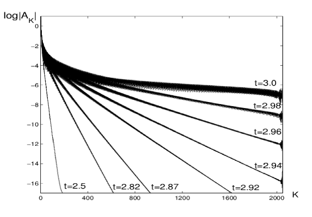
Figure 1: The behavior in time of the shell summed amplitude up to the singularity time.

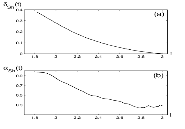
Figure 2: (a) The behavior in time of the width of the analyticity strip. The singularity time is $t_{c}\approx 3.0$. (b) The singularity is of cubic-root type.

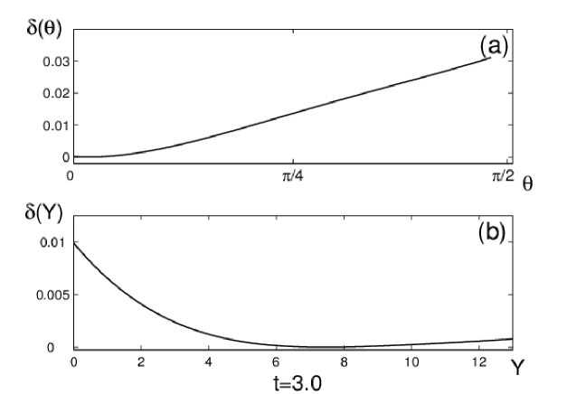
Figure 3: (a) The most singular direction is $\theta=0$. (b) If one estimates the $\delta$ in its dependence on the normal variable, one finds that the location of the singularity is at $Y\approx 7$.

In Fig. 4 we show the solution, at the singularity time, at the location $Y=7$ and in Fig. 5 it is show the behaviour in time of the spectrum at location $Y=7$. In Fig. 6 one can see the results of the singularity tracking method for the initial datum (2.5) at the location $Y=7$ obtained using the mixed spectral-finite difference numerical scheme.

All these results are consistent with those obtained with the fully spectral method. In Fig.6(c) one can see that the real tangential location of the singularity $x^{*}$, found with a study of the oscillatory behavior of the spectrum depurated by the exponential and algebraic decay, is consistent with the location of the shock shown in Fig. 5.

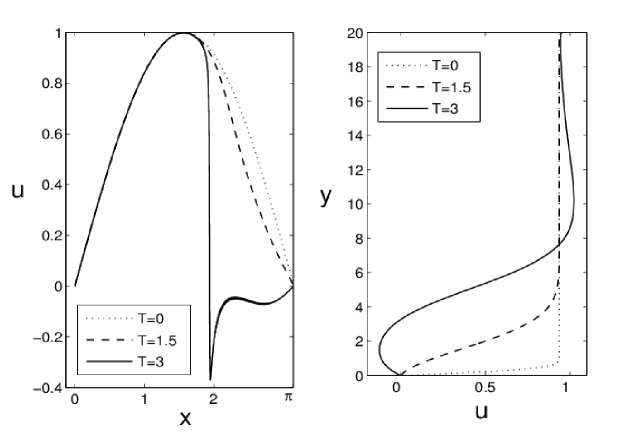
Figure 4: The solution of Prandtl’s equation at the location $Y=7$ for VanDommelen and Shen initial datum given by (2.5). To the left one can follow the formation of a shock at $x\approx 1.94$ at the location $Y=7$. The right figure shows the tangential velocity at the singularity location along the boundary layer.

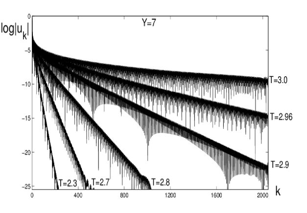
Figure 5: The spectrum of the solution of Prandtl’s equation at the location $Y=7$ with initial datum given by (2.5).

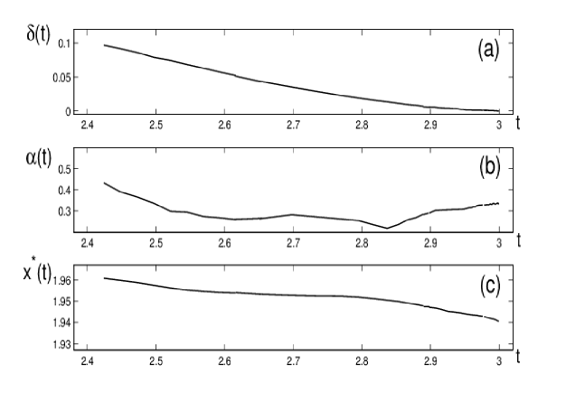
Figure 6: The results of the singularity tracking at $Y=7$. One can see that at $t\approx 3$ the strip of analyticity shrinks to zero as the result of a cubic–root singularity hitting the real axis. The location of the shock in Fig. 4 and the real coordinate of the singularity $x^{*}$ at the singularity time coincide.

4 Early singularity formation

In the rest os this paper we shall denote by $\mathcal{U}\equiv u^{VDS}(x,Y,t=1.5)$ the Van Dommelen and Shen solution (i.e. the solution of (2.1)–(2.4) with initial datum (2.5)) at the time $t=1.5$, well before the critical time. In this section we shall perturb this datum adding an analytic (in $x$) function that has a singularity at distance $\delta_{0}$ from the real axis. We shall show that the addition of this perturbation accelerates the formation of the singularity.

Let us introduce the family of real functions:

$$U_{\delta_{0}}(x)=\sum_{2\leq|k|\leq K/2}-i\frac{k}{|k|}\frac{e^{-\delta_{0}|k|}}{|k|^{5/3}}\cos{(x^{*}k)}e^{ikx},$$ (4.1)

The above functions are analytic in a strip of the complex plane of width $\delta_{0}$ and have a $2/3$–singularity at distance $\delta_{0}$ from the real axis. Moreover the fact that the spectrum oscillates as $\cos{(x^{*}k)}$ means that we are considering a dipole singularity, i.e. two $5/3$–singularities of opposite sign located at $x^{*}\pm\varepsilon+i\delta$ of strength $1/\varepsilon$ in the limit $\varepsilon\rightarrow 0$.

We now consider the following family of initial data for Prandtl’s equations (2.1)–(2.4).

$$u_{0}(x,Y)=\mathcal{U}+\sigma U_{\delta_{0}}f(Y)\;,$$ (4.2)

where $f(y)$ is a $C^{2}$ function of the form:

$$f(y)=\left\{\begin{array}[]{ll}y^{2}\exp{(-y)}&\mbox{for}\;0\leq y\leq 2\\ 4e^{-2}&\mbox{for}\;2\leq y\leq 3\\ 4e^{-2}\exp{\left[(-(y-3)/1.5)^{3}\right]}&\mbox{for}\;3\leq y\leq 20\end{array}\right.$$ (4.3)

This means that we are perturbing the VDS datum at $t=1.5$ placing a singularity at distance $\delta_{0}$ from the real axis. Moreover the role of the function $f(Y)$ is to make the strength of the singularity zero at the boundary and exponentially decaying far away from the the boundary. The maximum of the perturbation when $2\leq Y\leq 3$. The role of $\sigma$ is to tune the strength of the perturbation of the VDS datum. In all the calculations we shall present we have chosen $\sigma=6.6$. Moreover we have taken $x^{*}=2.17$ which is the real coordinate of the VDS singularity at $t=1.5$.

In Fig. 7 we compare the vorticity (defined as $-\partial_{Y}u$) of $\mathcal{U}$ (to the left) with the vorticity of the initial datum (4.2) with $\delta_{0}=0.025$ (to the right). From Fig. 7 it is evident that the effect of the perturbation $\sigma U_{\delta_{0}}f(Y)$ is to place a couple of counter rotating vortices in the boundary layer. One can see in Fig. 8 how these two vortices speed up the process of the vorticity stretching and the process of the singularity formation for Prandtl’s equations.

It is important to notice that the family of functions (B.10) when $\delta_{0}\geq 0$ is uniformly bounded in the norm $H^{1}$ (actually in $H^{s}$ when $s<7/6$).

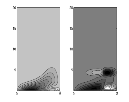
Figure 7: To the left the vorticity of the VDS solution at $t=1.5$. To the right the vorticity of the datum (4.2) with $\delta_{0}=0.025$.

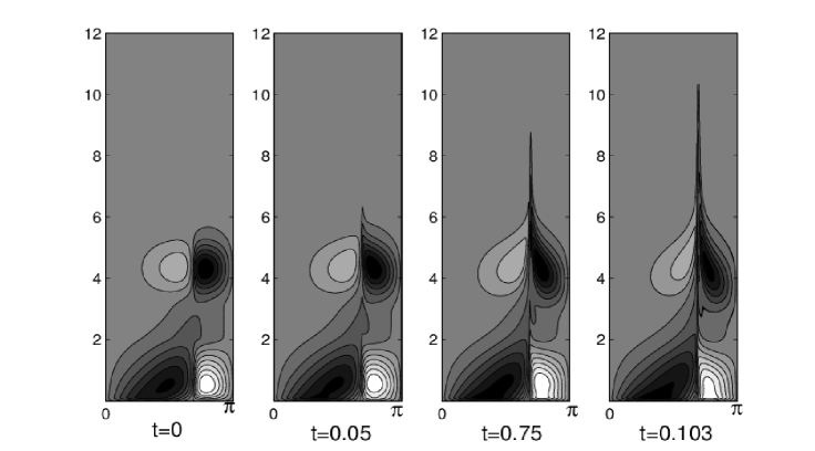
Figure 8: The vorticity $-\partial_{Y}u$ for Prandtl’s equations with initial datum (4.2) and $\delta_{0}=0.025$, at different times.

We now solve Prandtl’s equations (2.1)–(2.4) with initial datum given by (4.2) with $\delta_{0}=0.025$. The calculations we shall present here have been performed using a fully spectral method with resolution $2048^{2}$.

In Fig. 9 we show the shell-summed amplitudes, where it is evident the loss of exponential decay. Fitting these amplitudes we get the results shown in Fig. 10, where one can see that, at time $t\approx 0.103$, the solution loses analyticity as a cubic-root singularity hits the real axis. In Fig. 11(a) we show the angular dependence of $\delta$ and one can see that the most singular direction is $\theta=0$. This result allows to treat the normal variable as a parameter. At the bottom of the same figure we show the dependence of $\delta$ on $Y$, and one can see that $\delta(Y)$ attains its minimum at $Y\approx 5$.

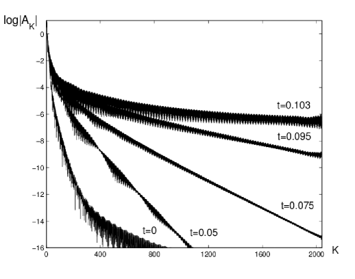
Figure 9: The behavior in time of the shell summed amplitude up to the singularity time.

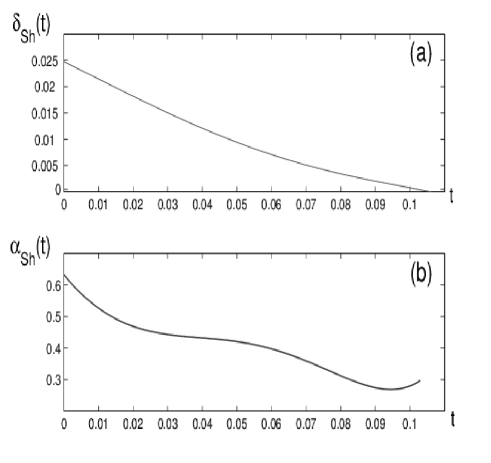
Figure 10: (a) The behavior in time of the width of the analyticity strip. The singularity time is $t_{c}\approx 0.103$. (b) The singularity is of cubic-root type.

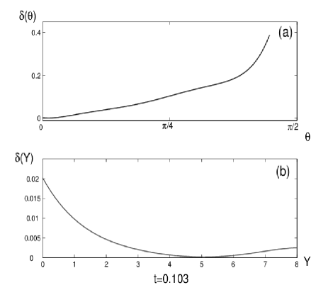
Figure 11: (a) As in the case of the Van Dommelen and Shen singularity, the most singular direction is $\theta=0$. (b) If one estimates the $\delta$ in its dependence on the normal variable, one finds that the location of the singularity is at $Y\approx 5$.

In Fig. 12 we show the solution, at the singularity time, at the location $Y=5$. In Fig.13 we show the results obtained using the mixed spectral-finite difference numerical scheme at the location $Y=5$. All these results are consistent with those obtained with the fully spectral method. In Fig.13(d) one can see that the real tangential location of the singularity $x^{*}$, found with a study of the oscillatory behavior of the spectrum depurated by the exponential and algebraic decay, is consistent with the location of the shock shown in Fig. 12(a).

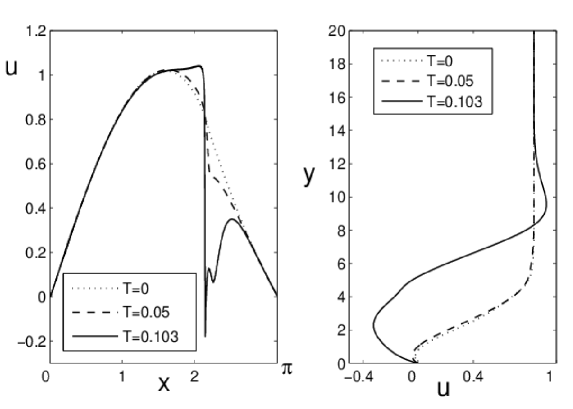
Figure 12: The solution of Prandtl’s equation at the location $Y=5$ with initial datum given by (4.2) with $\delta_{0}=0.025$. To the left one can follow the formation of a shock at $x\approx 2.14$ at the location $Y=5$. The right figure shows the tangential velocity at the singularity location along the boundary layer.

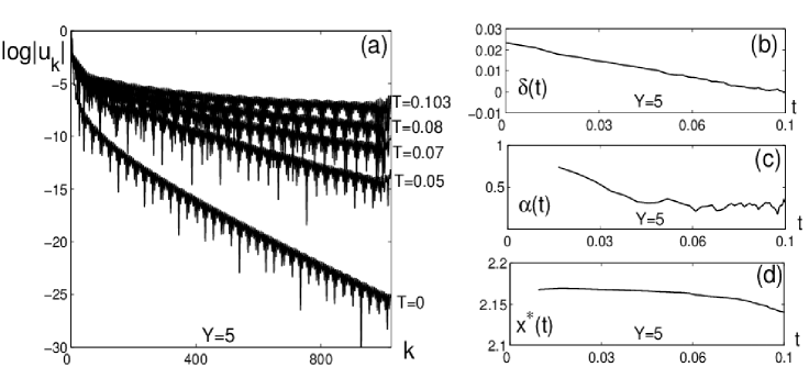
Figure 13: (a) The spectrum of the solution of Prandtl’s equation at the location $Y=5$ with initial datum given by (4.2) with $\delta_{0}=0.025$. (b) and (c) The results on the singularity time and on the type of the singularity, obtained fitting the spectrum at $Y=5$, are consistent with the results obtained using the shell-summed amplitudes. (d) The location of the shock in Fig.12 and the real coordinate $x^{*}$ of the singularity, at the blow-up time, coincide.

5 A case study: Burger’s equation

We now consider Burger’s equation:

$$\partial_{t}u+u\partial_{x}u=0\;,$$

with initial datum:

$$u(x,t=0)=\sin{(x)}+U_{\delta_{0}}\;,$$ (5.1)

with $U_{\delta_{0}}$ given by (B.10) where we have chosen $x^{*}=\pi$. At the top of Fig. 14 we show the behavior of the solution at various time for $\delta_{0}=0.1$. At the bottom one can see the behavior of the Fourier spectrum at various times. The loss of exponential decay of the spectrum is apparent. Moreover, the fact that the spectrum does not oscillate, clearly indicates that the real coordinate of the singularity remains $x^{*}(t)=\pi$.

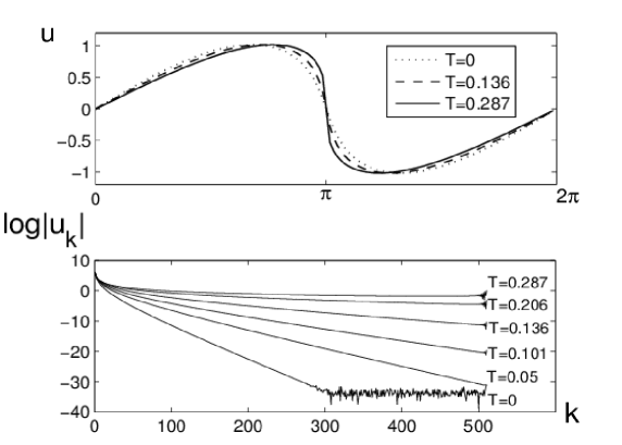
Figure 14: The behavior of the solution and the spectrum of Burger’s equation with initial datum (5.1) with $\delta_{0}=0.1$. A singularity in the form of a weak shock forms at $t\approx 0.287$.

At the top of Fig. 15 we are representing the shrinking in time of the analyticity strip for various $\delta_{0}$. At the bottom the evolution in time of the singularity type for different $\delta_{0}$. One can see that at the respective singularity times, the solutions form a square root singularity.

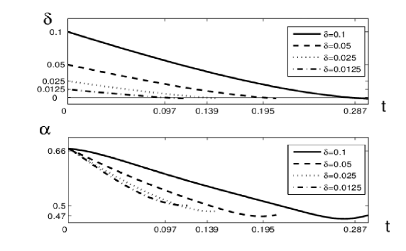
Figure 15: At the top the distances of the singularity from the real axis for different initial $\delta_{0}$s. At the bottom one can see that, at the singularity times, all the singularities have evolved in square–root singularities.

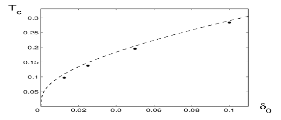
Figure 16: The singularity times for different $\delta_{0}$. The singularity time goes to zero when the $\delta_{0}$ goes to zero.

In Fig. 16 we compare the computed singularity times for different initial $\delta_{0}$ with the theoretical values of the critical times (the dashed line) In fact, for Burger’s equation, the singularity time is related to the inverse of $\sup_{x}|\partial_{x}u_{0}|$. For the initial data $u_{0}$ given by (5.1), one has:

$$\sup_{x}|\partial_{x}u_{0}|=1+\sum_{k>1}\frac{e^{-\delta_{0}k}}{k^{2/3}}.$$ (5.2)

Introducing the polylogarithm $Li_{s}(z)=\sum_{k\geq 1}\frac{z^{k}}{k^{s}}$ (see [1]), one can write the above formula as

$$\sup_{x}|\partial_{x}u_{0}|=1-e^{-\delta_{0}}+Li_{\frac{2}{3}}(e^{-\delta_{0}}).$$ (5.3)

The polylogarithm $Li_{s}(z)$ with $s=2/3$ is analytic for $|z|<1$ and divergent at $z=1$ This means that in the limit $\delta_{0}\rightarrow 0$, the derivative of the initial data $u_{0}$ becomes arbitrarily large and therefore the singularity time arbitrarily short. Therefore in the class of initial data (5.1) (which, as we previously noticed is uniformly bounded in $H^{1}$ when $\delta_{0}\geq 0$) the singularity time can be made arbitrarily short. The fact that the singularity evolves in a square-root singularity means that the solution, at the singularity time, it is not in $H^{1}$.

The situation is in fact different for the class of initial data:

$$u_{0}(x,y)=\sin{(x)}-\sum_{2\leq|k|\leq K/2}2i\frac{k}{|k|}\frac{e^{-\delta_{0}|k|}}{|k|^{5/2}}\cos{(x^{*}k)}e^{ikx},$$ (5.4)

These data, due to the different algebraic behavior of the spectrum (the complex singularities are in fact weaker), they are uniformly bounded in $H^{3/2}$ where the problem is well posed. This can be seen in Fig. 17 where one can see that these data still develop a square–root singularity, but the singularity time does not converge to zero when $\delta_{0}$ goes to zero.

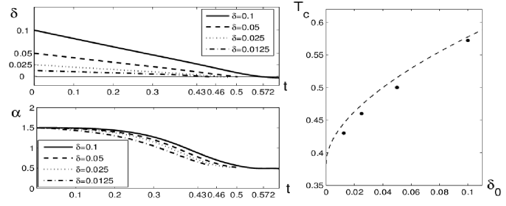
Figure 17: If one considers the class of initial data (5.4) one can see in the right figure that, however small the $\delta_{0}$ is taken, the time for which the solution becomes singular does not converge to zero. At the singularity time the solutions develop a square–root singularity (bottom left figure).

6 The singularity times for Prandtl’s equation

We now solve the Prandtl equations with the initial data (B.10) for different $\delta_{0}$. To give more reliability to our results we have tracked the singularities using also the sliding fitting technique. Instead of fitting the whole spectrum, one fits (using the asymptotic formula (2.11)) the spectrum starting from the mode $u_{k}$ up to the mode $u_{k+L}$. If the results (i.e. the $\delta$s and the $\alpha$s) are relatively insensitive to the $k$, this can be considered as an evidence of the genuineness of the results. In the calculations we show in Fig. 18 we have chosen $L=50$. Similar results have been obtained with different $L$. For other instances where the sliding fitting has been used, we refer to [8, 15, 16, 20, 33] and to reference therein.

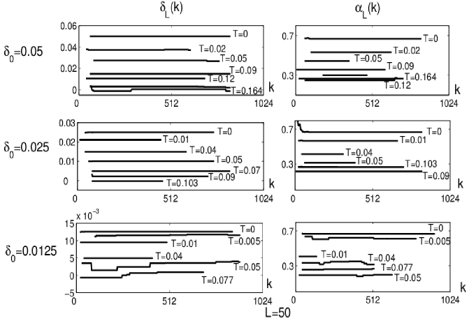
Figure 18: The results of the sliding fitting of the spectrum of the solution of Prandtl’s equation, at the location Y=5, with initial datum (4.2) and with different $\delta_{0}$. The left figures show the width of the analyticity strip as it goes to zero at the singularity times. To the right the algebraic classification of the singularities. At the singularity time they are all cubic–root singularities.

In Fig. 18 we use the sliding fitting technique to show the shrinking of the analyticity strip and the classification of the singularities at location $Y=5$ for various $\delta_{0}=0.05$, $0.025$, and $0.0125$. Note that, at the singularity times, are all cubic–root singularities, therefore stronger than the respective singularities for Burger’s equation. The results of the sliding fitting are in agreement with the results obtained fitting the whole spectrum represented (only the $\delta(t)$) at the top of Fig. 19.

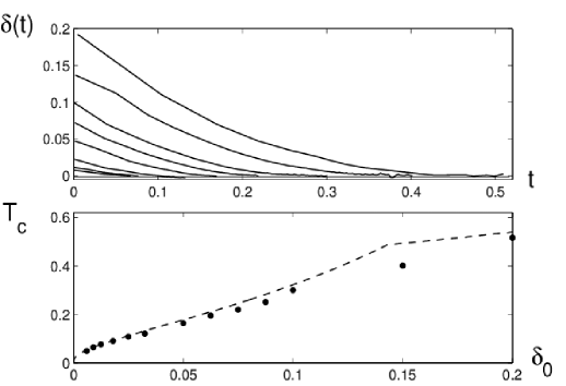
Figure 19: At the top the distances from the real axis of the singularity for Prandtl’s equation at the location $Y=5$ with initial datum given by (B.10), for different initial $\delta_{0}$s. At the bottom we compare the singularity times for different $\delta_{0}$ with the curve representing the $(\sup_{x,Y}|\partial_{x}u_{0}|)^{-1}$.

At the bottom of Fig 19 we plot (with a dashed line) the curve giving the dependence on $\delta_{0}$ of $1/\sup_{x,Y}|\partial_{x}u_{0}|$, where $u_{0}$ are the initial data expressed by (4.2). The computed singularity times seem to lay quite close to this curve. Therefore it seems to emerge a behavior of the singularity times similar to the behavior of Burger’s equation. Our findings reinforce the idea that the generation of the separation singularity for Prandtl’s equations is analogous to the wave steepening for compressible flow, and its connection to Burger’s equation (see [39]).

Moreover we found a class of initial data, uniformly bounded in norm $H^{1}$, for which our simulations seem to show that the singularity time can be made arbitrarily short. At the singularity time the solution has a strong discontinuity and it is not in $H^{1}$.

If one imposes an initial datum with a weaker singularity one gets a different behavior of the singularity times. In fact, we impose the initial data (4.2), where $U_{\delta_{0}}$ is now given by:

$$U_{\delta_{0}}(x)=\sum_{2\leq|k|\leq K/2}-i\frac{k}{|k|}\frac{e^{-\delta_{0}|k|}}{|k|^{5/2}}\cos{(x^{*}k)}e^{ikx}.$$ (6.1)

These initial data are uniformly bounded in $H^{3/2}$, for each initial $\delta_{0}\geq 0$; they develop a cube–root singularity within a finite time, as one can see in Fig. 20, where we report the case of $\delta_{0}=0.05$. In Fig. 21 one can see that, also in this case, the singularity times seem to be related to $1/\sup_{x,Y}|\partial_{x}u_{0}|$. This would mean that, in this class of initial data, the blow–up time of the derivative of the solution does not go to zero when $\delta_{0}\rightarrow 0$.

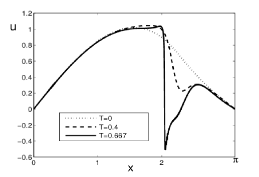
Figure 20: The solution of Prandtl’s equation at the location $Y=5$ with initial datum given by (6.1) with $\delta_{0}=0.05$. To the left one can follow the formation of a shock at $x\approx 2.14$ at the location $Y=5$. To the right the results of the singularity tracking. One can see that at $t\approx 0.667$ the solution develops a cubic–root singularity at the real coordinate $x^{\star}\approx 2.14$.

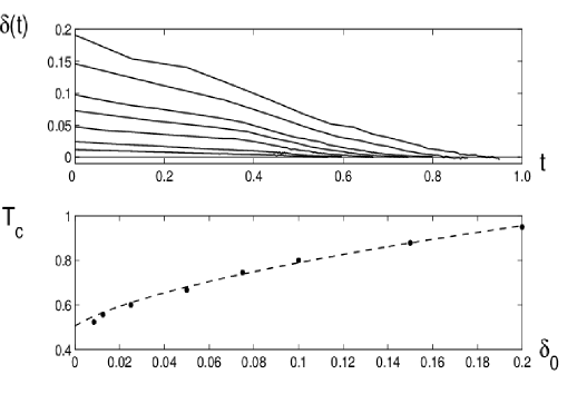
Figure 21: At the top the distances from the real axis of the singularity for Prandtl’s equation at the location $Y=5$ with initial datum given by (6.1), for different initial $\delta_{0}$s. At the bottom the singularity times for different $\delta_{0}$s. The singularity time seem to lay on the curve $(\sup_{x,Y}|\partial_{x}u_{0}|)^{-1}$. This would mean that the singularity time remains bounded away from zero when $\delta_{0}\rightarrow 0$.

7 The regularized Prandtl’s equation

We now consider the effects of a small viscosity in the streamwise direction on the process of the singularity formation. Namely we consider the equations:

$$\partial_{t}u+u\partial_{x}u+v\partial_{Y}u-U\partial_{x}U = \partial_{YY}u+\nu\partial_{xx}u\qquad U=\sin{(x)}$$ (7.1)

$$\partial_{x}u+\partial_{Y}v = 0$$ (7.2)

$$u(x,0,t)=v(x,0,t) = 0$$ (7.3)

$$u(x,\infty,0) = U$$ (7.4)

with initial datum:

$$u(x,y,0)=\sin{(x)}\,.$$ (7.5)

We solve the above equation with the methods we have used for the Prandtl’s equation (described in Section 2) plus the usual spectral discretization of the viscous term $(\partial_{xx}u)_{k}=-k^{2}u_{k}$ treated implicitly in time. The scheme has good convergence properties, at least below a certain resolution.

In fact, if we now follow the distance of the singularity from the real axis of the singularity, we get the results of Fig. 22, where the results for different values of the viscosity are represented. The resolution used for the computation of Fig. 22 is $K=1024$ in $x$ and $M=800$ in $Y$. For the computations we have used a $32$-digits precision.

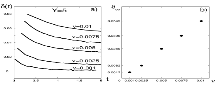
Figure 22: Imposing the impulsively started disk datum, one can see that the singularities do not hit the real axis (at least up to times $T=5$, well after the VDS singularity time $t=3$) but stabilize at a distance $\delta_{\infty}$ which depends on the amount of viscosity in the streamwise direction. To the right it seems to emerge a linear dependence of $\delta_{\infty}$ (which is related to the number of Fourier modes effectively excited) on the viscosity $\nu$.

One can therefore see that the regularized Prandtl’s equations, solved up to time $T=5$ well after the VDS singularity time, stay regular. Moreover the singularity seems to stabilize at a distance of the real axis that depends on the viscosity in $x$. Plotting the distances that the singularities reach asymptotically in time versus the viscosity it seems to emerge a linear dependence. This suggests that, if $d$ is the number of degrees of freedom necessary to describe the behavior of the regularized Prandtl’s equations, then $d\sim\nu^{-1}$. In Fig. 23 we plot the solution $u$ at the location $Y=5$ at different times. One can see how the solution steepens to form a regularized shock.

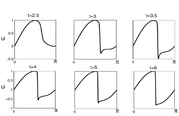
Figure 23: The solution of the regularized Prandtl’s equations starting from the initial datum $u_{0}=\sin{(x)}$. The effect of the viscosity $\nu=0.005$ in the streamwise direction is to regularize the solution. One can see the steepening of the solution at $Y=5$ and the formation of a regularized shock.

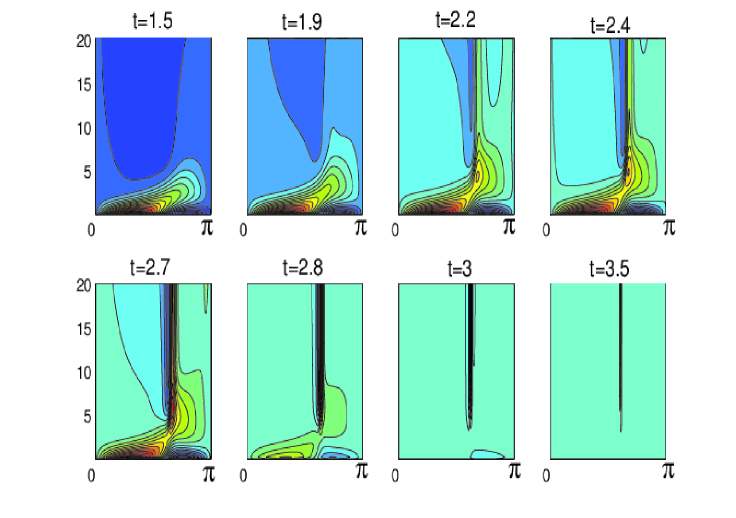
Figure 24: Vorticity contours for the regularized Prandtl’s equations with $\nu=0.005$ starting from the initial datum $u(x,Y,t=0)=\sin{(x)}$. The detachment of the vorticity from the boundary is evident and the formation of two strips of high vorticity of opposite sign is reminiscent of VDS singularity.

In Fig. 24 we have represented the contours of the vorticity $\omega=-\partial_{Y}u/\sqrt{\nu}+\sqrt{\nu}\partial_{x}v$ at various times. Vorticity detaches from the boundary and, asymptotically, two strips of vorticity of opposite sign are formed. These two strips are the result of the steepening of the solution throughout the boundary layer as shown in Fig. 23 at $Y=5$.

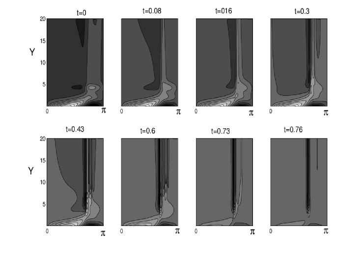
Figure 25: Instantaneous vorticity $\omega=-\partial_{Y}u/\sqrt{\nu}+\sqrt{\nu}\partial_{x}v$ contours of the solution of the regularized Prandtl’s equations for $\nu=0.005$ having imposed the initial datum (4.2) with $\delta_{0}=0.2$. Looking at $t=0$ it clarifies that the effect of the analytic perturbation $U_{\delta_{0}}$ is to place a pair of counter-rotating vortices inside the boundary layer. Notice how vorticity detaches from the boundary to feed one of the two vortices. Asymptotically it forms two strips of vorticity of opposite sign.

In Fig. 25 we see the vorticity contours starting from the initial datum (4.2) with $\delta_{0}=0.2$. Comparing the vorticity at $t=0$ in Fig. 25 with the vorticity at $t=1.5$ of Fig. 24 one realizes that the effect of the complex singularity we have added to the VDS datum at $t=1.5$ reveals as a couple of counter rotating vortices places in the boundary layer. These two vortices speed up the process of the vorticity detachment from the boundary and the process of the formation of the high vorticity strip, as it is apparent from a comparison between Fig. 24 and Fig. 25.

We finally notice that to resolve the regularized Prandtl’s equation it is necessary to use a number $K$ of modes in $x$ such that $K\gtrsim 1/\delta_{\infty}$. In fact if the singularity gets to a distance from the real axis smaller than the resolution in $x$, this would result in the formation of spurious oscillations and in the ultimate blow up of the computed solution.

8 Conclusions

The singularity tracking method has revealed an effective tool to investigate the dynamics of the boundary layer equations. The process leading to Van Dommelen and Shen’s singularity has revealed itself as the results of a complex cubic–root singularity (coming from infinity) hitting the real axis (of the complexified $x$ variable) at time $t\approx 3$. We have seen how this process can be accelerated perturbing the boundary layer solution with a datum containing a singularity (the dipole singularity) at distance $\delta_{0}$ from the real axis. Moreover we have seen that it seems possible to make the singularity time short at will picking the initial datum in a class uniformly bounded in the norm $H^{1}_{x}\times C^{2}_{Y}$. The critical time for Prandtl’s equations (in its dependence from $\delta_{0}$ as $\delta_{0}$ is taken smaller) seems to behave as it does the critical time of Burger’s equation for similar initial data, see Fig. 19 at the bottom. We stress that at the singularity time the solution is not in $H^{1}$, being the singularity of the cubic–root type, see Fig.s 18 at the right. The well posedness of the Prandtl’s equations has been proved for analytic (in $x$) initial data or for monotonous initial data. The question of the well posedness (or of the ill posedness) in Sobolev spaces is an important question that remains open. The findings of this paper (especially if supported by calculations at higher resolution which would allow to consider initial singularities increasingly closer to the real axis) suggest that the well posedness (if possible) needs regularity in $x$ higher than $H^{1}$.

The introduction in Prandtl’s equations of a small viscosity in the streamwise direction prevents the formation of the singularity (at least for the viscosities that we have been able to test). In fact the complex singularity instead of hitting the real axis, after a transient during which it gets closer to the real axis, it stabilizes at a distance $\delta_{\infty}$ which depends (linearly, it seems) on the amount of regularizing viscosity. Being $\delta_{\infty}$ related to the number of the Fourier modes effectively excited, this indicates a finite dimensional dynamics of the 2D regularized Prandtl’s equations. We believe it would be interesting to confirm (or disprove) this at smaller viscosity (which requires higher resolution) and/or in a 3D setting. We finally notice that the solution of the regularized Prandtl’s equations for relatively large times requires, due to the growth of the boundary layer, to consider a larger computational domain in the normal direction; or, alternatively, the coupling with the Euler or the Navier–Stokes equations at the outer boundary. This, and other topics, will be the subject of future work.

Appendix A Appendix: E and Engquist’s singularity

In this appendix we analize the singularity formation for Prandtl’s equation for an analytic initial datum given firstly by E and Engquist [18], and to determinate its complex characterization. We remember that the work of E and Engquist (EE) is the only analytic existing result about the blow–up for solutions of Prandtl’s equation at a finite time. We point out some differences between EE singularity and the separation singularity which accous in VanDommelen and Shen situation analized in section 3. We consider here a periodic version of the work of E and Engquist, which is simple to obtain.

We consider the periodic Prandtl’s equation in the domain $D=[-\pi,\pi]\times[0,\infty]$

$$\partial_{t}u+u\partial_{x}u+v\partial_{Y}u = \partial_{YY}u,$$ (A.1)

$$\partial_{x}u+\partial_{Y}v = 0,$$ (A.2)

$$u|_{Y=0}=v|_{Y=0} = 0,\qquad u\rightarrow 0\quad\mbox{when}\quad Y\rightarrow\infty\;$$ (A.3)

$$u|_{x=-\pi} = u|_{x=\pi},$$ (A.4)

$$u|_{t=0} = u_{0}=-\sin(x)b_{0}(x,Y),$$ (A.5)

where the outer Euler inviscid flow is imposed to be zero, and where $b_{0}\geq 0$ is a regular function of $x$ and $y$ in $D$, not necessarily periodic in $x$, which satisfies the following condition

$$E(a_{0})=\int_{0}^{\infty}\left(\frac{1}{2}(\partial_{Y}a_{0})^{2}-\frac{1}{4}a_{0}^{3}\right)dY<0;$$ (A.6)

with $a_{0}=b|_{x=0}\geq 0$. E and Engquist prove that there exists a finite time $T$ such that the $x$–derivative of the solution $u$ of Prandtl equations blow up. In particular, this means that we have $\lim_{t\rightarrow T}\sup_{Y>0}|\frac{u(x,Y,t)}{\sin x}|_{x=0}=+\infty$ or otherwise

$$\lim_{t\rightarrow T}\sup_{Y>0}|\partial_{x}u(0,Y,t)|=+\infty.$$ (A.7)

Like in section 3 for the VDS’s initial datum, we solve numerically Prandtl’s equation (A.1)–(A.4), with inital datum given by (A.5) and

$$b_{0}(x,Y)=a_{0}(Y)=\frac{1}{4}Y^{2}e^{-(Y-2)},$$ (A.8)

which satisfies condition (A.6). In figures (26) it is show the behavior in time of the solutions for Prandtl’s equation with initial datum given by (A.5) and (A.8). In this case the flows corresponds to flows impinging from the left and right at the line $x=0$, which is the rear stagnation point.

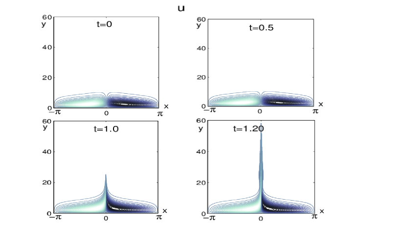
Figure 26: The streamwise velocity $u$ of Prandtl’s equation with initial datum given by (A.8). One can follow the formation of a shock at $t\approx 1.20$.

At time $t\approx 1.20$ Gibb’s phenomenons are visible for the velocity $u$, so we argue that Prandtl’s equation develops a singularity at this time. As the singularity forms, the singular structure seems to be convected to $Y=+\infty$, making the numerical computations difficult. We have considered the computational domain as $[-\pi,\pi]\times[0,Y_{\mbox{\tiny MAX}}]$, and we chose $Y_{\mbox{\tiny MAX}}=60$ where the velocity $u$ is of the order of $10^{-18}$ at time $t\approx 1.20$.

In the figure on the left of Fig.27 we show the behavior of $a(Y,t)=\partial_{x}u(0,Y,t)$, as one can see at time $t\approx 1.20$ the maximum grows around the location $Y\approx 20$. On the right of figure Fig.27 we show the profile at different times of $u$ at the location $Y=20$ where the maximum of $a$ seems to be reach.

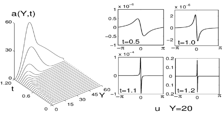
Figure 27: On the right figure the behavior of the function $a(Y,t)=\partial_{x}u(0,Y,t)$ for solution of Prandtl’s equation with initial datum (A.8). On the left the profiles of $u$ at the cut $Y=20$ and at different times.

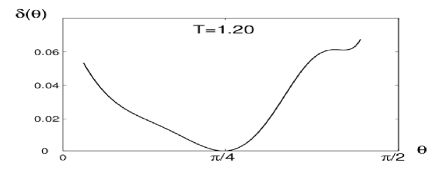
Figure 28: The profile of the distance $\delta$ at the singularity time w.r.t. the angle $\theta$ for the solution of Prandtl’s equation with initial datum (A.8), at the singularity time $t=1.20$. The distance $\delta$ seems to reach its minimum at $\approx\pi/4$.

In figure Fig.28 it is shown the behavior of the strip of analyticity $\delta$ with respect to the angle $\theta$ at the singularity time $t=1.20$. As one can see, this case is quite different from the VDS–singularity. In this case the distance $\delta$ seems to reach a minimum at $\approx\pi/4$, and this means that the influence for the complex singularity by the $Y$ variable is not neglecting for the EE singularity. In this case the technique of singularity tracking to detecting the location and the algebraic type of the complex singularity at different cuts of $Y$ does not work, then we analyze the behavior in time of the corresponding shell–summed Fourier amplitude [27] $A_{K}$ defined in the subsection 2.4. In Fig.29 we show the evolution of $A_{K}$ at different times. In Fig.30, one can see the distance $\delta$ which reach the real axis at the time $t=1.20$ and $\alpha$ is equal to $1/3$. This confirm the formation of a shock singularity in the $x$ derivative for the solution of Prandtl’s equation with an EE type initial datum given by (A.8).

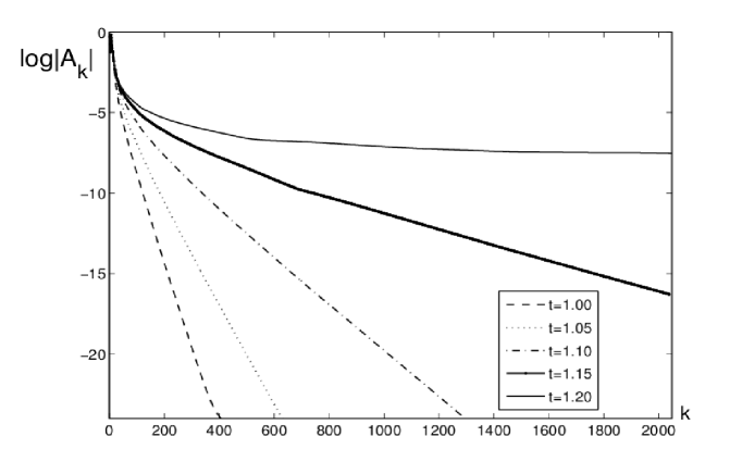
Figure 29: The time evolution of the shell–summed amplitude of the fourier spectrum for Prandtl’s equation with initial datum given by (A.8).

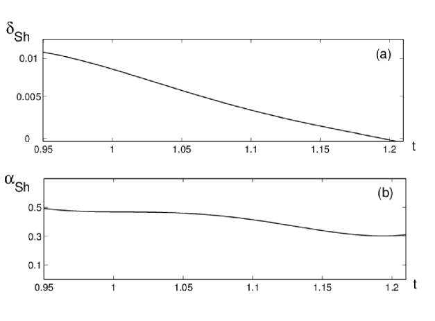
Figure 30: The singularity tracking results for the solution of Prandtl’s equation with initial datum given by (A.8). In $(a)$ and $(b)$ the respective evolutions in time of the distance $\delta$ and the algebraic factor $\alpha$.

Finally, we point out that if we choose another type of exponential decaying at infinity, the results are similar. As a conclusion we said that the EE singularity developed by the initial datum (A.8), analyzed in this section seems to be a shock–singularity in the $\partial_{x}u$, like in the classical VDS case. Moreover, the situation is different from the VDS case for some aspects. First of all, no recirculation region forms. The flow remains separated at the rear stagnation point where the singularity develops, different from the VDS case where the flow separates from the boundary at approximately $3\pi/4$ from the front stagnation point. As second step, the complex singularity in the EE case depends not only by the streamwise variable like in VDS, but also by the normal variable, as we point out in this appendix.

Appendix B Appendix: Perturbation at the Euler outer flow

In this appendix we shall investigate the response to perturbation at both the initial datum and Euler outer flow of the VDS case, adding an analytic function in $x$ that has a singularity at distance $\delta_{0}$ from the real axis, as doing in section 4. Also in this situation, the addition of a perturbation accelerates the formation of the singularity. Moreover, the algebraic structure of shock singularity remains stable, i.e. differents initial configurations devolops singularity at different times but all have the same shock type of singularity observed for the VDS case.

We consider the following family of initial data and the Euler outer flows $U$ for Prandtl’s equations (2.1)–(2.4), with

$$u_{0}(x,Y)=U(x)=U_{(\delta_{0},\alpha_{in},x^{*},\sigma)}\;,$$ (B.9)

where

$$U_{(\delta_{0},\alpha_{in},x^{*},\sigma)}(x)=\sin(x)+\sigma\sum_{2\leq|k|\leq K/2}-i\frac{k}{|k|}\frac{e^{-\delta_{0}|k|}}{|k|^{\alpha_{in}+1}}\cos{(x^{*}k)}e^{ikx}.$$ (B.10)

We now solve Prandtl’s equations (2.1)–(2.4) with initial datum and Euler outer flow given by (B.9) (B.10) with differentes $\delta_{0}$, $\alpha_{in}$, $\sigma$ and $x^{*}$. The calculations we shall present here have been performed using a fully spectral method with resolution $2048^{2}$.

We present in Fig. 31 and Fig. 32, the fitting of the shell–summed amplitude for differents initial configurations. As one can see, all the solutions lose analyticity at finite time and have the same cubic-root singularity.

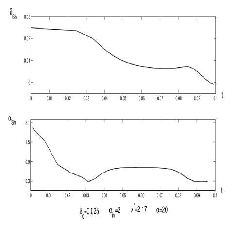
Figure 31: The behavior in time of the width of the analyticity strip for initial and Euler outer flow given by (B.9) with $\delta_{0}=0.025$, $\alpha_{in}=2$, $\sigma=20$ and $x^{*}=2.17$. The singularity time is $t_{c}\approx 0.098$, and the singularity is of cubic-root type.

Figure 32: The behavior in time of the width of the analyticity strip for initial and Euler outer flow given by (B.9) with differents initial configurations of $\alpha_{in}$ and $\sigma$, at the same $x^{*}=0$ and $\delta_{0}=0.1$. All the singularities are of cubic-root type.

We point out that for initial $x^{*}=0$, the $x$–location of the singularity is different from zero, as one can see in Fig. 33 were we show the shell-summed amplitudes with $\delta_{0}=0.1$, $\alpha_{in}=3/2$, $\sigma=20$ and $x^{*}=0$. It is evident the loss of exponential decay and the formation of oscillations at the singularity time.

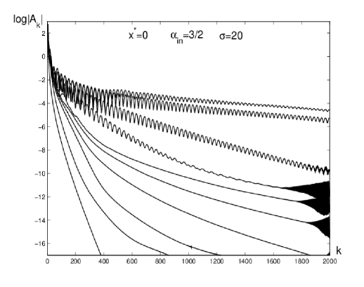
Figure 33: The behavior in time of the shell summed amplitude up to the singularity time, for initial and Euler outer flow given by (B.9) with $\delta_{0}=0.1$, $\alpha_{in}=3/2$, $\sigma=20$ and $x^{*}=0$.

References

- [1] M. Abramowitz and I. A. Stegun, Handbook of Mathematical Functions, Dover, New York, 1972.
- [2] K. Asano, Zero Viscosity Limit of the Incompressible Navier–Stokes Equations 1 and 2, preprint, (1988).
- [3] U. Ascher, S. Ruuth, and R. Spiteri, Implicit–explicit Runge–Kutta methods for time–dependent partial differential equations, Appl. Numer. Math., 25 (1997), pp. 151–167.
- [4] D. Bailey, H. Yozo, X. Li, and B. Thompson. ARPREC: An arbitrary precision computation package, (September 1, 2002). Lawrence Berkeley National Laboratory. Paper LBNL-53651.
- [5] C. Bardos and È. S. Titi, Euler equations for an ideal incompressible fluid, Uspekhi Mat. Nauk, 62 (2007), pp. 5–46.
- [6] J. P. Boyd, Chebyshev and Fourier spectral methods, Dover Publications Inc., Mineola, NY, second ed., 2001.
- [7] K. Brinckman and J. Walker, Instability in a viscous flow driven by streamwise vortices, J. Fluid. Mech., 432 (2001), pp. 127–166.
- [8] R. Caflisch, Singularity formation for complex solutions of the 3D incompressible euler equations, Phisica D, 67 (1993), pp. 1–18.
- [9] R. Caflisch and M. Sammartino, Existence and Singularity for the Prandtl Boundary Layer Equations, Z. Angew Math. Mech, 80 (2000), pp. 733–744.
- [10] M. Cannone, M. Lombardo, and M. Sammartino, Existence and Uniqueness for the Prandtl Equations, C.R. Acad. Sci. Paris Sér I Math, 332 (2001), pp. 277–282.
- [11] C. Canuto, M. Y. Hussaini, A. Quarteroni, and T. A. Zang, Spectral methods: Fundamentals in single domains, Scientific Computation, Springer-Verlag, Berlin, 2006.
- [12] G. Carrier, M. Krook, and C. Pearson, Functions of a Complex Variable: Theory and Technique, McGraw–Hill, New York, 1966.
- [13] K. Cassel, A comparison of Navier-Stokes solutions with the theoretical description of unsteady separation, R. Soc. Lond. Philos. Trans. Ser. A Math. Phys. Eng. Sci., 358 (2000), pp. 3207–3227.
- [14] S. Cowley, Laminar Boundary-Layer Theory: A 20th Century Paradox?, in Mechanics for a New Millennium, Proceedings of 20th ICTAM, H. Aref and J. Phillips, eds., New York, 2001, Springer, pp. 389–411.
- [15] S. Cowley, G. Baker, and S. Tanveer, On the formation of Moore curvature singularities in vortex sheets, J. Fluid. Mech., 378 (1999), pp. 233–267.
- [16] G. Della Rocca, M. C. Lombardo, M. Sammartino, and V. Sciacca, Singularity tracking for Camassa-Holm and Prandtl’s equations, Appl. Numer. Math., 56 (2006), pp. 1108–1122.
- [17] W. E, Boundary layer theory and the zero–viscosity limit of the Navier–Stokes equations, Acta Math. Sin., 16 (2000), pp. 207–218.
- [18] W. E and B. Engquist, Blowup of the Solutions to the Unsteady Prandtl’s Equations, Comm. Pure Appl. Math., 50 (1997), pp. 1287–1293.
- [19] U. Frisch, T. Matsumoto, and J. Bec, Singularities of Euler Flow? Not out of the Blue!, J. Stat. Phys., 113 (2003), pp. 761–781.
- [20] R. Goldstein, A. Pesci, and M. Shelley, Instabilities and singularities in Hele–Shaw flow, Physics of Fluids, 10 (1998), pp. 2701–2723.
- [21] E. Grenier, On the stability of boundary layers of incompressible euler equations, J. Differential Equations, 164 (2000), pp. 180–222.
- [22] L. Hong, A Numerical and Analytic Study of the Prandtl Equations, PhD dissertation, Univerity of California, Davis, Dept. of Mathematics, 2002.
- [23] L. Hong and J. Hunter, Singularity Formation and Instability in the Unsteady Inviscid and Viscous Prandtl Equations, Comm. Math. Sci., 1 (2003), pp. 293–316.
- [24] D. Ingham, Unsteady separation, J. Comp. Phys., 53 (1984), pp. 90–99.
- [25] T. Kato, Remarks on the zero viscosity limit for nonstationary navier-stokes flows with boundary, in Seminar on nonlinear partial differential equations, no. 2 in Math. Sci. Res. Inst. Publ., Springer, New York, 1984, pp. 85–98.
- [26] M. Lombardo, M. Cannone, and M. Sammartino, Well–Posedness of the Boundary Layer Equations, SIAM J. Math. Anal., 35 (2003), pp. 987–1004.
- [27] T. Matsumoto, J. Bec, and U. Frisch, The Analytic Structure of 2D Euler Flow at Short Times, Fluid Dyn. Res., 36 (2005), pp. 221–237.
- [28] A. Obabko and K. Cassel, On the ejection–induced instability in Navier–Stokes solutions of unsteady separation, Phyl. Trans. R. Soc. A, 363 (2005), pp. 1189–1198.
- [29] O. Oleinik, On the Mathematical Theory of Boundary Layer for an Unsteady flow of Incompressible Fluid, J. Appl. Math. Mech., 30 (1966), pp. 951–974.
- [30] O. Oleinik and V. Samokhin, Mathematical models in boundary layer theory, vol. 15 of Applied Mathematics and Mathematical Computation, Chapman & Hall/CRC, Boca Raton, FL, 1999.
- [31] W. Pauls and U. Frisch, A Borel transform method for locating singularities of Taylor and Fourier series, J. Stat. Phys., 127 (2007), pp. 1095–1119.
- [32] W. Pauls, T. Matsumoto, U. Frisch, and J. Bec, Nature of Complex Singularities for the 2D Euler Equation, Physica D, 219 (2006), pp. 40–59.
- [33] M. Pugh and M. Shelley, Singularity Formation in Thin Jets with Surface Tension, Comm. Pure Appl. Math., 51 (1998), pp. 733–795.
- [34] M. Sammartino and R. Caflisch, Zero Viscosity Limit for Analytic Solutions of the Navier–Stokes Equations on a Half–Space I: Existence for Euler and Prandtl Equations, Comm. Math. Phys., 192 (1998), pp. 433–461.
- [35] , Zero viscosity limit for analytic solutions of the Navier–Stokes equations on a half–space II: Construction of the Navier–Stokes solution, Comm. Math. Phys., 192 (1998), pp. 463–491.
- [36] M. Shelley, A study of singularity formation in vortex–sheet motion by a spectrally accurate vortex method, J. Fluid. Mech., 244 (1992), pp. 493–526.
- [37] C. Sulem, P.-L. Sulem, and H. Frisch, Tracing Complex Singularities with Spectral Methods, J. Comput. Phys., 50 (1983), p. 138 161.
- [38] R. Temam and X. Wang, The convergence of the solutions of the Navier-Stokes equations to that of the Euler equations, App. Math. Lett., 10 (1997), pp. 29–33.
- [39] L. Van Dommelen, Unsteady Boundary Layer Separation, PhD dissertation, Cornell University, 1981.
- [40] L. Van Dommelen and S. Cowley, On the Lagrangian description of unsteady boundary-layer separation. I. General theory, J. Fluid Mech., 210 (1990), pp. 593–626.
- [41] L. Van Dommelen and S. Shen, The Spontaneous Generation of the Singularity in a Separating Laminar Boundary Layer, J. Comp. Phys., 38 (1980), pp. 125–140.
- [42] , The Genesis of Separation, in Symposium on Numerical and Physical Aspects of Aerodynamic Flows, T. Cebeci, ed., Springer, 1982, pp. 293–311.
- [43] Z. Xin and L. Zhang, On the Global Existence of Solutions to the Prandtl’s System, Adv. Math., 181 (2004), pp. 88–133.