Goal oriented adaptivity in the IRGNM for parameter identification in PDEs II:
all-at once formulations
B. Kaltenbacher
A. Kirchner
B. Vexler
Abstract
In this paper we investigate adaptive discretization of the iteratively regularized Gauss-Newton method IRGNM. All-at-once formulations considering the PDE and the measurement equation simultaneously allow to avoid (approximate) solution of a potentially nonlinear PDE in each Newton step as compared to the reduced form [22]. We analyze a least squares and a generalized Gauss-Newton formulation and in both cases prove convergence and convergence rates with a posteriori choice of the regularization parameters in each Newton step and of the stopping index under certain accuracy requirements on four quantities of interest. Estimation of the error in these quantities by means of a weighted dual residual method is discussed, which leads to an algorithm for adaptive mesh refinement. Numerical experiments with an implementation of this algorithm show the numerical efficiency of this approach, which especially for strongly nonlinear PDEs outperforms the nonlinear Tikhonov regularization considered in [21].
1 Introduction
We consider the problem of identifying a parameter in a PDE
(1)
from measurements of the state
(2)
where , , , are Hilbert spaces and
with denoting the dual space of some Hilbert space and differential and observation operators, respectively.
Among many others, for example the classical model problem of identifying the diffusion coefficient in the linear elliptic PDE
from measurements of in can be cast in this form with , , , and the embedding of into .
The usual approach for tackling such inverse problems is to reduce them to an operator equation
(3)
where is the composition of the parameter-to-solution map for (1)
(4)
with the measurement operator .
The forward operator will then be a nonlinear operator between and with typically unbounded inverse, so that recovery of is an ill-posed problem.
Since the given data are noisy with some noise level
(5)
regularization is needed.
We will here as in [22] consider the paradigm of the Iteratively Regularized Gauss-Newton Method (IRGNM) cf., e.g.,
[3, 4, 7, 18, 20, 23] and its adaptive discetization.
However, instead of reducing to (3), we will simulteously consider the measurement equation and the PDE:
(6)
(7)
as a system of operator equations for , which we will abbreviate by
(8)
where
(9)
The noisy data for this all-at-once formulation is denoted by
This will allow us to avoid a major drawback of the method in [22], namely the necessity of solving the possibly nonlinear
PDE (to a certain precision) in each Newton step in order to evaluate .
Another key difference to the paper [22] is that here the part of the previous iterate will not be subject to new discretization in the current iteration but keep its (usually coarser, hence cheaper) discretization from the previous step.
Therewith, we will arrive at iterations of the form
(10)
with , .
For ,
this yields a least squares formulation, see Section 2.
In case and sufficiently large, by exactness of the norm with exponent one as a penalty, this leads to a Generalized Gauss-Newton type [8] form of the IRGNM
Although obviously depend on , i.e. ,
we omit the superscript for better readability.
All-at-once formulations have also been considered, e.g., in [1, 2, 9, 10],
however, our approach focuses on adaptive discretization using a posteriori error estimators. Additionally it differs from the previous ones
in the following sense: In [9, 10] a Levenberg-Marquardt approach is considered, whereas we work with
an iterative regularized Gauss-Newton approach which allows us to also prove convegergence rates (which is an involved task in a Levenberg-Marquardt
setting, that has been resolved only relatively recently, [16]). Moreover we use a different regularization parameter choice in each Newton
step than [9, 10]. The papers [1, 2] put more emphasis on computational aspects and
applications than we do here.
For both cases , in (10) we will investigate convergence and convergence rates in the continuous and adaptively discretized
setting with discrepancy type choice of (which in most of what follows will be replaced by ) and the overal stopping index . The discretization errors with respect to certain quantities of interest will serve as refinement criteria during the Gauss-Newton iteration, where at the
same time, we control the size of the regularization parameter. In order to estimate this discretization error we use goal-oriented error estimators (cf. [5, 6]).
For the least squares case we will (for the sake of completeness but not in the main steam of this paper) also provide a result on convergence with a priori
parameter choice in the continuous setting, see the appendix.
In Section 4, we will provide numerical results and in Section 5 some conclusions.
Throughout this paper, we will make the following assumptions:
Assumption 1.
There exists a solution to
(8), where is some initial guess and (not to be confused with the penalty parameter in (10))
is the radius of the neighborhood in which local convergence of the Newton type iterations under consideration will be shown.
Assumption 2.
The PDE (1) and especially also its linearization
at is uniquely and stably solvable.
Assumption 3.
The norms in , , as well as the operator and the semilinear form defined by the relation
(where denotes the duality pairing between and )
are assumed to be evaluated exactly.
2 A least squares formulation
Direct application of the IRGNM to (6), (7), i.e., to the all-at-once system (8)
yields the iteration
(14)
(17)
with regularization parameters , for the and part of the iterates, respectively.
We will first of all show that Assumption 2 allows us to set the regularization parameter for the part to zero.
For this purpose, we introduce the abbreviations
(18)
with Hilbert space adjoints and , i.e.,
(19)
where and denote the inner products in and .
In the same way we define the Hilbert space adjoint for , i.e.,
Motivated by Lemma 1, and setting we define a regularized iteration by
(29)
(32)
or equivalently as solution to the unconstrained minimization problem
(33)
with the abbreviations
(34)
where we have set the regularization parameter for the
component to zero, which is justified by (i) in Lemma 1.
The optimality conditions of first order for (33) read
We refer to the Appendix for a convergence and convergence rates results for (32) with a priori choice of the regularization parameters and in a continuous setting.
Here we are rather interested in a posteriori parameter choice rules and adaptive discretization.
So in each step we will replace the infinite dimensional spaces in (32) by finite dimensional ones
(35)
where is the previous iterate, which itself is discretized by the use of spaces .
The discretization may be different in each Newton step (typically it will get finer for increasing ), but we suppress dependence of on in our notation in most of what follows.
To still obtain convergence of these discretized iterates, it is essential to control the discretization error in certain quantities, which are defined, analogously to [22], via the functionals
where we insert the previous and current iterates , , respectively:
(36)
and quantities of interest
(37)
Their discrete analogs are correspondingly defined by
(38)
and
(39)
At the end of each iteration step we set
(40)
Remark 2.
Note that here neither nor are subject to new adaptive discretization in the current step, but
they are taken as fixed quantities from the previous step. This is different from [22],
where also depends on the current discretization.
For (37) and (39) we assume that the
norms in and are evaluated exactly cf. Assumption 3.
In our convergence proofs we will compare the quantities of interest with those that would be obtained with exact computation on the infinite dimensional spaces, starting from the same as the one underlying . Thus, in our analysis besides the actually computed sequence there appears an auxiliary sequence , see Figure 1.
Figure 1: Sequence of discretized iterates and auxiliary sequence of continuous iterates for the
all-at-once formulation of IRGNM
We assume the knowledge about bounds on the error in the quantities of interest due to discretization
(41)
(, which can, at least partly, be computed by goal oriented error estimators, see e.g., [5, 6, 14, 21]
and Section2.1)
and to refine adaptively according to these bounds. On the other hand, we will now impose conditions on such upper bounds for the discretization error that enable to prove convergence and convergence rates results, see Assumption 7 below.
Additionally, we will make some assumptions on the forward operator
Assumption 4.
Let the reduced forward operator be continuous and weakly sequentially closed, i.e.
for all sequences .
We also transfer the usual tangential cone condition to the all-at once setting from this section, which yields
Assumption 5.
Let
hold for all and some .
The choice of the regularization parameter will be done a posteriori according to an inexact Newton /discrepancy principle, which with the quantities introduced above reads as
(42)
A discrepancy type principle will also be used for the choice of the overall stopping index
(43)
The parameters used there have to satisfy the following assumption.
Assumption 6.
Let and be chosen sufficiently large and sufficiently small
(see (42),(43)), such that
(44)
Therewith, we can also formulate our conditions on precision in the quantities of interest:
Assumption 7.
Let for the discretization error with respect to the quantities of interest estimate (41) hold,
where , , , are selected such that
(45)
(46)
(47)
for some constants , and a sequence as (where the second condition in (47)
is possible due to the right inequality in (44)).
Exactly along the lines of the proofs of Theorems 1 and 2 in in [22], replacing there by according to (9), we therewith obtain convergence and convergence
rates results:
Theorem 1.
Let the Assumptions 1, 2, 3, 4 and 5
with sufficiently small be satisfied and let Assumption 6 hold.
For the quantities of interest (37) and (39),
let, further, the estimate (41) hold with satisfying Assumption 7.
Then with , fulfilling (42), selected according to (43), and
defined by (35) there holds
(i)
(48)
(ii)
is finite ;
(iii)
converges (weakly) subsequentially to a solution of (8) as
in the sense that it has a weakly convergent subsequence and each
weakly convergent subsequence converges strongly to a solution of (8).
If the solution to (8) is unique, then
converges strongly to as .
For proving rates, as usual (cf. e.g. [4, 11, 18, 23]) source conditions are assumed
Assumption 8.
Let
(cf. Assumption 1)
hold with some such that is strictly monotonically increasing on
,
defined by is convex and defined by
is strictly monotonically increasing on
.
Here, for some selfadjoint nonnegative operator , the operator function is defined via functional calculus based on the spectral theorem (cf. e.g. [11]).
Theorem 2.
Let the conditions of Theorem 1 and additionally
the source condition Assumption 8
be fulfiled.
Then there exists a and a constant independent of such that
for all
the convergence rates
(49)
are obtained.
Remark 3.
We compare the source conditions for the reduced formulation
(50)
with Assumption 8 for the
all-at-once formulation, e.g. in the case .
Namely, in that case
(50) reads: There exists such that
(51)
On the other hand,
Assumption 8 with the same reads: There exists
such that
which is equivalent to
and by elimination of and use of the identities and
we get
Theoretically the error estimators for this subsection can be computed similarly to those from
[22]. The fact that we consider an unconstrained optimization problem should make things
easier, but we get another problem in return: For estimating and we would have to estimate terms
like
for some operator , which would be quite an effort to do via goal oriented error estimators.
For this reason, the presented least squares formulation will not be implemented
and we will not go into more detail concerning the error estimators for this section.
3 A Generalized Gauss-Newton formulation
A drawback of the unconstrained formulation (33) is the necessity of computing the -norm
of the (linearized) residual and especially of computing error estimators for this quantity of interest.
Besides, a rescaling of the state equation (7) changes the solution of the optimization problem.
Moreover, depending on the given inverse problem and its application, in some cases, it does not make sense to only minimize
the residual of the linearized state equation, instead of setting it to zero.
A formulation that is much better tractable is obtained by defining as a solution to the PDE
constrained minimization problem
We will prove inductively that the iterates indeed remain in , see estimate (73) below. Thus, due to Lemma 2,
which remains valid in the discretized setting (62), we get uniform boundedness of the dual variables by some sufficiently large , namely
(60)
Hence we can use exactness of the norm with exponent one as a penalty (cf., e.g., Theorem 5.11 in [13]), which implies that a solution of (52), (53) coincides with the unique solution of the unconstrained minimization problem
(61)
for larger than the norm of the dual variable.
The formulation (61) of (52), (53) will be used in the convergence proofs only. For a practical implementation we will directly discretize (52), (53).
(cf. (37)),
where , are fixed from the previous step and , are coupled by the linearized state equation (53)
(or the third line of (LABEL:eq_IRGNM_KKT_sqp) respectively)
for and .
Consistently, the discrete counterparts to (64) and (65)
are
(66)
and
(67)
(cf. (39)), where are fixed from the previous step,
since (like in (40)) we set and
at the end of each iteration step.
Remark 4.
Here, as compared to (37), we have removed the -norms in the
definition of and .
The -norm still appears in , but only in connection
with the old iterative , such that the only source of error in is the evaluation
of the norm. That means that with respect to Section 2, we have replaced
the problematic expression
for arbitrary , where is a third order remainder term
(see e.g. [5, 6], Section 3.1).
Please note that due to the relation (71) no additional system of equations has to be solved
in order to obtain the additional variable .
Another way to deal with the discretization error in is the following: Tracking the upcoming
convergence proof (cf. Theorem 3) the reader should realize that the discretization
for does not have to be the same as for , , such that
could be evaluated on a very fine separate mesh, such that could be neglected. This alternative is
of course, more costly, but since everything else is still done on the adaptively refined (coarser) mesh,
the proposed method could still lead to an efficient algorithm.
The -norm also appears in , and unfortunately, in combination with the current and ,
which are subject to discretization, such that in principle we face the same situation as in the least squares formulation
from Section 2 (cf. Subsection 2.1). Since, however, only appears in connection with the very
weak assumption as (cf. (46)), as in [22], we save ourselves the computational
effort of computing an error estimator for .
Like in Section 2 we need the weak sequential closedness of , i.e. Assumption 4
and the following tangential cone condition (cf. Assumption 5).
By means of Lemma 2 and the Assumptions 4,
10
we can now formulate a convergence result like in Theorems 1 and 3 in [22] and Theorem 1 here
for (52). This can be done similarly to the proof of Theorem 3
in [22], replacing there by according to (9) and setting
(72)
there. For clarity of exposition we provide the full convergence proof (Theorem 3) without making use of the equivalence to (61) here.
Only for the convergence rates result Theorem 4 we refer to Theorem 4 in [22] with (72) and the equivalence to (61).
So in the proof of Theorem 3 we will not use minimality wrt (61) but only wrt the original formulation (52), (53) (actually we are using KKT points instead of minimizers, but this make no real difference due to convexity of the problem).
Theorem 3.
Let the Assumptions 1, 2, 3, 4 and 10
with sufficiently small be satisfied and let Assumption 6 hold.
For the quantities of interest (65) and (67),
let, further, the estimate (41) hold with satisfying Assumption 7.
Then with , fulfilling (42), selected according to (43), and
defined as the primal part of a KKT point of
(62), (63) there holds
(i)
(73)
(ii)
is finite ;
(iii)
converges (weakly) subsequentially to a solution of (8) as
in the sense that it has a weakly convergent subsequence and each
weakly convergent subsequence converges strongly to a solution of (8).
If the solution to (8) is unique, then
converges strongly to as .
We mention in passing that this is a new result also in the continuous case .
Proof.
(i):
We will prove (73) by induction. The base case is trivial.
To carry out the induction step, we assume that
(74)
holds. We consider a continuous step emerging from discrete ,
(cf. Figure 1),
i.e. let be a solution to (52) for
.
Then the KKT conditions
(cf. (54)-(56)) imply
for all and , where we have used the same abbreviations as in (34) and
(59), as well as defined by (58).
Setting , , this yields
where we have used the fact that satisfies the linearized state equation (53),
i.e.
Hence by Cauchy-Schwarz and the fact that for all
which dividing by 2 and applying Lemma 2 with (60),
and (74) leads to
(75)
for all .
The rest of the proof basically follows the lines of the proof of Theorem 3
in [22]
with the choice (72), but for convenience of the reader we will follow through the proof
anyway.
Using the fact that for all and Assumption 10 from
(75) we get
for all .
This together with (42) and
the fact that
yields
By the triangle inequality as well as (42),
Assumption 10 and the fact that satisfies the linearized state equation (53),
we have
which implies
From this, using (41) and (47) we can deduce exactly as in the proof of Theorem 3 (ii) in [22] that
(76)
with
(77)
So since the right hand side of (76) tends to zero as , and therewith (cf. (47)) eventually has to fall below for some finite index .
(iii):
With (5), (41), (46) and the definition of , we have
(78)
as . Thus, due to (ii) (73)
has a weakly convergent subsequence
and with Assumption 4 and (78) the limit of every weakly
convergent subsequence is a solution to (8).
Strong convergence of any weakly convergent subsequence again follows by a
standard argument like in [22] using (73).
∎
Corollary 1.
The sequence is bounded, i.e.
Proof.
The assertion follows directly from Theorem 3 (i) and Lemma 2.
∎
The convergences rates from Theorem 4 in [22] also hold for the all-at-once formulation (8), due to equivalence with (61) which we
formulate in the following theorem.
Instead of source conditions we use variational source conditions (cf., e.g., [12, 19, 20, 26]) due to the nonquadratic penalty term in (61).
Assumption 11.
Let
(80)
with sufficiently large (cf. (60)) and independent from ,
hold with some such that is strictly monotonically increasing on
,
defined by is convex and defined by
is strictly monotonically increasing on
.
Theorem 4.
Let the conditions of Theorem 3 and additionally
the variational inequality Assumption 11 be fulfilled.
Then there exists a and a constant independent of such that
for all ß
the convergence rates
(81)
with ,
are obtained.
Proof.
With (72) the rate follows directly from Theorem 4 in [22]
due to Theorem 3
(especially (73))
and (78).
∎
Remark 5.
In fact, no regularization of the part would be needed for proving just stability of the single Gauss-Newton steps,
since by Assumption 2 the terms
and in (61) as regularization term together ensure weak compactness of the level sets of the Tikhonov functional (cf. Item 6 in Assumption 2 in [22]). However, we require even uniform boundedness of in order to uniformly bound the dual variable and come up with a penalty parameter that is independent of , cf. the discrete version of Lemma 2.
Using
the equality constraint (53) (for )
together with the tangential cone condition Assumption 10 for
would only enable to bound :
such that
However, without error estimators on the difference between
and its discretized version, this does not give a recursion
(from which, by uniform boundedness of and Assumption 9 we could conclude uniform boundedness of ).
Thus, in order to obtain uniform boundedness of we introduce the term here for theoretical purposes.
For our practical computations we will assume that the error by discretization between
and is small enough so that the mentioned gap in this argument for uniform boundedness of can be neglected and the part of the regularization term is omitted.
3.1 Computation of the error estimators
Since – different to [22] – ist not subject to new discretization in the th step here, the computation of the error estimators is easier and can be done exactly as in
[14] and [21]. Thus we omit the arguments and in the quantities of
interest in this subsection and we also omit the iteration
index and the explicit dependence on .
Error estimator for :
We consider
and the Lagrange functional
(82)
with and defined as
and
There holds a similar result to Proposition 1 in [22](see also [14]), which
allows to estimate the difference by computing a discrete stationary point
of . This is done by solving the equations
Please note that the equations (83)-(85) are solved anyway in the process of solving the optimization problem (52), (53).
Error estimator for :
The computation of the error estimator for can be done similarly to the computation of
in [22] (or in [14]) by means of
the Lagrange functional . We consider
and compute a discrete stationary point of the auxiliary
Lagrange functional
by solving the equations
(87)
(with ). Then we compute the error estimator for by
Remark 7.
To avoid the computation of second order information in (87) we would like to refer to [6], where
(87) is replaced by an approximate equation of first order.
Error estimator for :
In Remark 4, we already mentioned that the norm in can be evaluated on a
separate very fine mesh, so that we will neglect the difference between and
. This implies that we do not need to compute the error estimator
, since , so that (47), and the first part of (46)
is trivially fullfilled.
Error estimator for :
We also mentioned in Remark 4 that we will not compute , as the error
needs to be controlled only through the very weak assumption
as (cf. (46)), which in practice we will simply make sure by altogether decreasing the mesh size in the course of the iteration.
3.1.1 Algorithm
Since we only know about the existence of an upper bound of (cf.
Corollary 1), but not its value, we choose (cf. (60)) heuristically, i.e. in each iteration step
we set for the discrete counterpart of .
Remark 8.
Theoretically one should use on a very fine discretization in order to get a better approximation to . However, since we only need the correct order of magnitude and not the exact value, we just
use the current mesh .
In view of Remark 5 we omit the part of the regularization term.
Also, as motivated in Section 3.1, we assume for all , such that
we neither compute nor .
For simplicity, we evaluate on the current mesh instead of a very fine mesh as explained in Remark 4.
For computing , fulfilling (42), we can resort to the Algorithm from [14], which also contains refinement with respect to the quantity of interest and repeated solution of
(90)
for .
The presented Generalized Gauss-Newton formulation can be implemented according to the following
Algorithm 1.
Algorithm 1.
Generalized Gauss-Newton Method
1: Choose , , , , such that and
Assumption 6 holds.
and ,
and choose , and , such that the second part of
(47) is fulfilled.
2: Choose a discretization and starting value
(not necessarily coinciding with in the regularization term)
and set .
3: Choose starting value (e.g. by solving the PDE
)
and set .
4: Compute the adjoint state
(see (55)),
evaluate , set .
and evaluate (cf. (39)).
11: With , fixed,
apply the Algorithm from [14] (with quantity of interest and noise level )
starting with the current mesh to obtain a regularization parameter and a possibly different discretization
such that (42) holds; Therwith, also the corresponding
, according to (90) are computed.
16: Refine grid with respect to such that we obtain a finer discretization
.
17: Solve the the optimization problem (90)
and evaluate .
18: Set .
19: Set , .
20: Compute the adjoint state
(see (55)), evaluate
, set .
and evaluate .
21: Set (i.e. use the current mesh as a starting mesh for the next iteration).
22: Set .
Remark 9.
In practice, we replace the “while”-loop on lines 15-19 of Algorithm 1 and in the Algorithm from [14]
which only serve as refinement loops by an “if”-condition in order to prevent over-refinement.
Since we want to either refine or make a Gauss Newton step, lines 15-19 are replaced by
2: Refine grid with respect to such that we obtain a finer discretization
3:.
4:else
5: Set , .
The structure of the loops is the same as in Algorithm 1 from [22], but here, we only have to solve linear PDEs (i.e. Step 6 in Algorithm 4 in [22]
is replaced by
“Solve linear PDE”), which justifies the drawback of one additional loop in comparison to
[21] (see also Algorithm 5 in [22].
This motivates the implementation and assumes
the gain of computation time for strongly nonlinear problems, which will be considered in terms of
numerical tests in Section 4.
4 Numerical Results
For illustrating the performance of the proposed method according to Algorithm 1,
we apply it to the example PDE
where we aim to identify the parameter from noisy measurements
of the state
in , where is a given constant. As for the measurements we consider two cases:
(i)
via point functionals in uniformly distributed points , and
perturbed by uniformly distributed random noise of some percentage . Then the observation space is chosen as and
the observation operator is defined by for .
(ii)
via -projection. Then , , and
where denotes some uniformly distributed random noise and the percentage of perturbation. The exact state
is simulated on a very fine mesh with nodes and equally sized quadratic cells, and we denote the corresponding finite element space by .
In order to evaluate on coarser meshes and the
corresponding finite element spaces with during the optimization algorithm, has to
be transferred from to the current grid . As usual in the finite element context, this is done by the -projection
as the restriction operator.
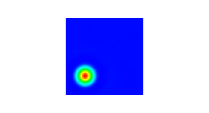
We consider configurations with three different exact sources :
(a)
A Gaussian distribution
with , , , and .
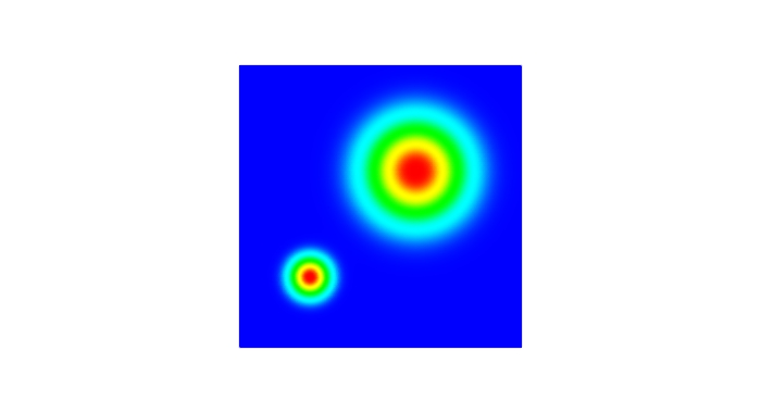
(b)
Two Gaussian distributions added up to one distribution
where
with , , , , , and .
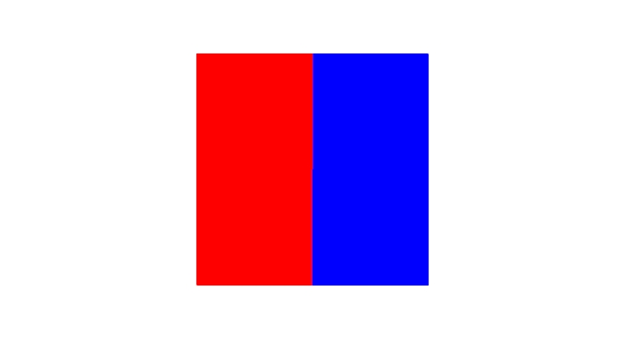
(c)
The step function
The concrete choice of the parameters for the numerical tests is as follows:
, , , , ,
, (, ). The coarsest (starting mesh) consists
of 25 nodes and 16 equally sized squares, the inital values for the control and the state
are and and we start with a regularization parameter .
Considering the numerical tests, we are mainly interested in saving computation time compared to the Algorithm from [21], where the inexact Newton
method for the determination of the regularization parameter is applied directly to the nonlinear problem, instead
of the linearized subproblems (90). That is why besides the numerical results for the Generalized Gauss-Newton (GGN)
method presented in section 3, we also present the results from the “Nonlinear Tikhonov” (NT) Algorithm from [21].
The choice of the parameters for (NT) is the following: , ,
, , , , . This setting implies that both algorithms (NT) and (GGN) are
stopped, if the concerning quantities of interest fall below the same bound ( for (NT) and
for (GGN)).
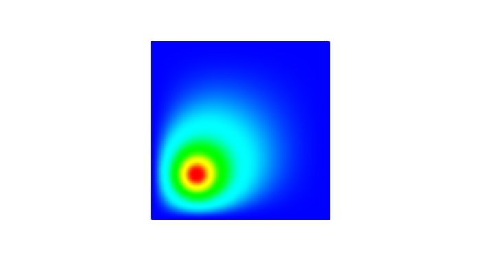
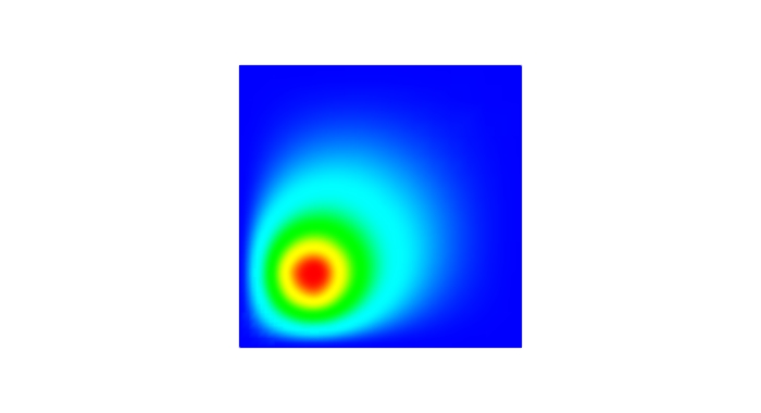
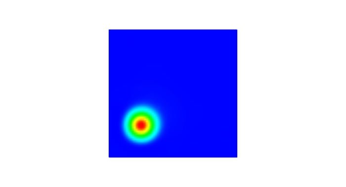
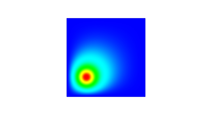
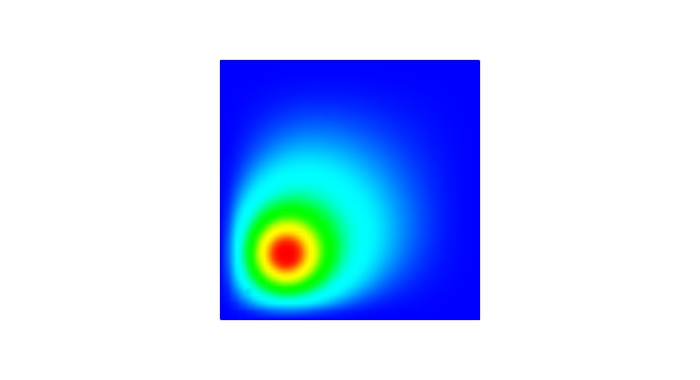
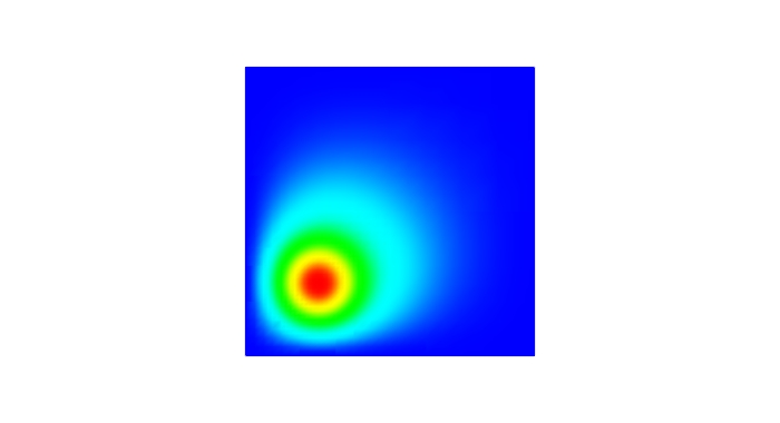
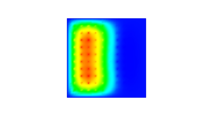
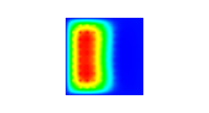
Figure 2: FLTR: exact control , reconstructed control by NT, reconstructed control by GGN
for example (a) (i) with , noise
Figure 3: FLTR: exact state , reconstructed state by NT, reconstructed state by GGN
for example (a) (i) with , noise
Figure 4: FLTR: adaptively refined mesh by NT , adaptively refined mesh by GGN
for example (a) (i) with , noise
The figures 2 and 3 show the exact source distribution and the corresponding simulated state
, as well as the reconstructions of the control and the state obtained by Algorithm 1 (GGN),
as well as the ones obtained by the algorithm from [21] (NT) for the example (a)(i) with and noise. In Figure 4 we see the very fine mesh for simulating the data,
the adaptively refined mesh obtained by (NT), and the adaptively refined mesh obtained by (GGN).
In table 1 we present the respective results for different choices of (first column). In the second and fifth column one can see the relative
control error , in the third and sixth column is the number of nodes in the adaptively refined mesh,
and in the forth and seventh column one can see the regularization parameter obtained by (GGN) and (NT) respectively. The eigthth column shows the
gain of computation time using (GGN) instead of (NT). The higher the factor is, the more computation time we save with (GGN). This is probably due
to the higher number of iterations needed for “more nonlinear” problems. Already for the choice replacing the nonlinear PDEs by linear ones
(getting an additional loop in return cf. subsection 3.1.1) seems to pay off. In that case (GGN) refines more than (NT)
(see Figure 4), but it is still faster (see table 1). For higher and (GGN)
is even much faster than (NT), because in addition to the cheaper linear PDEs, it also refines less. At the same time, the relative control error
is about the same as with (NT).
Table 1: Algorithm 1 (GGN) versus the algorithm from [21] (NT)
for Example (a)(i) for different choices of with noise. CTR: Computation time reduction using (GGN) in comparison to (NT)
NT
GGN
CTR
error
# nodes
error
# nodes
1
0.418
2985
2499
0.412
4600
3873
-65%
10
0.417
3194
2473
0.411
4918
3965
-59%
100
0.408
5014
6653
0.417
6773
9813
39%
500
0.418
9421
11851
0.404
13756
821
97%
1000
0.439
11486
44391
0.426
16355
793
99%
In table 2 the reader can see the results for the same example with for different noise levels using (GGN).
The numerical results confirm what we would expect: the larger the noise, the larger the error, the stronger the
regularization, the coarser the discretization.
Table 2: Example (a)(i) for different noise levels with
noise
error
# nodes
0.5%
0.385
12260
9867
1%
0.417
6773
9813
2%
0.553
1687
413
4%
0.700
599
137
8%
0.937
42
137
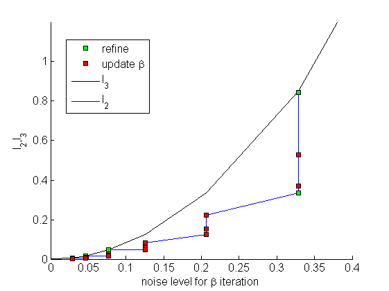
Figure 5: Behavior of (GGN) for example (a)(i) with and noise
Taking a look at Figure 5 the reader can track the behavior of Algorithm 1 (GGN)
for the considered example (a)(i) with and noise. The algorithm goes from right to left
in Figure 5, where the quantities of interest and (or rather their discrete counterparts
and ) are rather large. The noise level for the inner iteration is about in the beginning.
For this noise
level the stopping criterion for the -algorithm (step 10,11 in Algorithm 1)
is already fulfilled, such that only one Gauss-Newton step is made without refining or updating .
This decreases the noise level to about . Then the -algorithm comes into play,
with one refinement step, two -steps and again one refinement step, which in total reduces
from to , with which the -algorithm terminates. The subsequent run of the -algorithm
consists only of three -enlargement steps and finally after Gauss-Newton iterations, both quantites
of interest and fulfill the required smallness conditions such that the whole Gauss-Newton Algorithm terminates.
Due to the observation above concerning the nonlinearity of the PDE,
we restrict our considerations to the case for the rest of this section.
The figures 6, 7, and 8
again show the results for example (a) with noise, but for the case (ii), i.e. via -projection.
Figure 6: FLTR: exact control , reconstructed control by NT, reconstructed control by GGN
for example (a) (ii) with , noise
Figure 7: FLTR: exact state , reconstructed state by NT, reconstructed state by GGN
for example (a) (ii) with , noise
Figure 8: FLTR: adaptively refined mesh by NT , adaptively refined mesh by GGN
for example (a) (ii) with , noise
(GGN) yields a regularization parameter , a discretization with nodes and a relative control error of .
(NT) leads to a much larger error of , a finer discretization with nodes and a much larger regularization parameter .
Although (GGN) refines only a little less than (NT), (GGN) is much faster than (NT), namely .
Compared to the point measurement evaluation, the -projection causes smoother solutions, which seem to reconstruct the exact data better,
but at the same time this is probably the less realistic case with respect to real applications.
In the figures 9 and 10, we can see the results using (GGN) and (NT)
for a different source, namely example (b) with point measurements (i) and again and noise. Since we are interested in idenfying the parameter
, we take a pass on presenting the reconstructed states and only show the reconstructed controls, as well as the adaptively refined meshes.
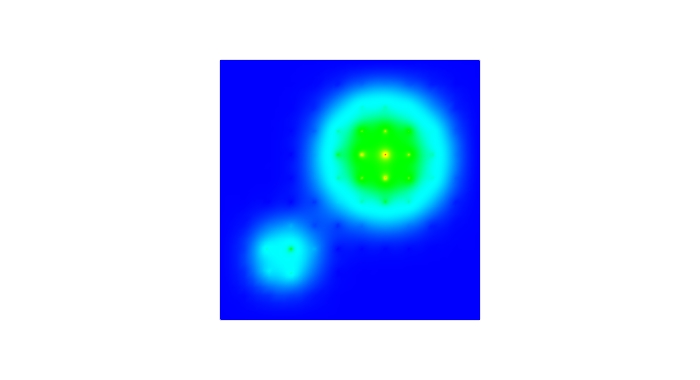
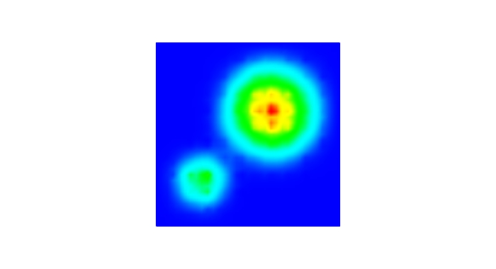
Figure 9: FLTR: exact control , reconstructed control by NT, reconstructed control by GGN
for example (b) (i) with , noise
Figure 10: FLTR: exact (very fine) mesh, adaptively refined mesh by NT , adaptively refined mesh by GGN
for example (b) (i) with , noise
(GGN) stops with a regularization parameter , a mesh with nodes, and a reconstruction yielding a relative error of ,
whereas (NT) terminates with , nodes and a larger error of .
Due to the much coarser discretization obtained by (GGN), it is not surprising, that we save about of computation time in this case.
The corresponding results for the source (c) are shown in Figure 11 and Figure 12.
Figure 11: FLTR: exact control , reconstructed control by NT, reconstructed control by GGN
for example (c) (i) with , noise
Figure 12: FLTR: exact (very fine) mesh, adaptively refined mesh by NT , adaptively refined mesh by GGN
for example (c) (i) with , noise
Using (GGN) we obtain a regularization parameter , a discretization with nodes and a relative control error of , while
(NT) yields , nodes and an error of . Also for this configuration (GGN) is faster than (NT), if only .
To put this in perspective, we would like to mention that the step function (c) is a very challenging example, since
the intial guess and the source have different values on the boundary.
Moreover, for piecewise constant functions total variation regularization is known to yield much better results than regularization.
5 Conclusions and Remarks
In this paper we consider all-at-once formulations of the iteratively regularized
Gauss-Newton method and their adaptive discretizations using a posteriori error estimators.
This allows us to consider only the linearized PDE (instead of the full potentially nonlinear one)
as a constraint in each Newton step, which safes computational effort. Alternatively, in a least squares approach,
the measurement equation and the PDE are treated simultaneously via unconstrained minimization of the squared
residual. In both cases we show convergence and convergence rates which we carry over to the discretized setting
by controlling precision only in four real valued quantities per Newton step. The choices of the regularization
parameters in each Newton step and of the overall stopping index are done a posteriori, via a discrepancy type
principle. From the numerical tests we have seen, that the presented method yields reasonable reconstructions and
can even lead to a large reduction of computation time compared to similar non-iterative methods.
6 Acknowledgments
The authors would like to thank the Federal Ministry of Education and Research (BMBF) for financial
support within the grant 05M2013 “ExtremSimOpt: Modeling, Simulation and Optimization of Fluids in Extreme Conditions”,
as well as the German Science Foundation (DFG) for their support within the grant KA 1778/5-1 and VE 368/2-1 “Adaptive Discretization
Methods for the Regularization of Inverse Problems”.
References
[1]U. Ascher and E. Haber,
A multigrid method for distributed parameter estimation problems,
ETNA 15, (2003), 1–12.
[2]G. Biros and O. Ghattas,
Parallel Lagrange-Newton-Krylov-Schur Methods for PDE-Constrained Optimization. Part I: The Krylov-Schur Solver,
SIAM Journal on Scientific Computing, 27 (2005) 687–713
[3]A. B. Bakushinskii,
The problem of the convergence of the iteratively regularized Gauss-Newton method,
Comput. Math. Math. Phys. 32 (1992), 1353–1359.
[4]A.B. Bakushinsky and M. Kokurin:
Iterative Methods for
Approximate solution of Inverse Problems. Kluwer Academic
Publishers, Dordrecht, 2004.
[5]R. Becker, R. Rannacher,
An Optimal Control Approach to a-Posteriori Error Estimation
Acta Numerica 2011 ed. A Iseries, (Cambridge University Press), 1–102.
[6]R. Becker, B. Vexler,
A posteriori error estimation for finite element discretizations of parameter identification problems
Numer. Math. 96 (2004), 435–59
[7]B. Blaschke(-Kaltenbacher), A. Neubauer, O. Scherzer,
On convergence rates for the iteratively regularized Gauß–Newton
method,
IMA J. Numer. Anal. 17 (1997), 421–436.
[8]H.-G. Bock,
Randwertproblemmethoden zur Parameteridentifizierung in Systemen nichtlinearer Differentialgleichungen,
Bonner Mathematische Schriften 183, Bonn, 1987.
[9]M. Burger and W. Mühlhuber:
Iterative regularization of parameter identification problems by sequential quadratic programming methods,
Inverse Problems 18 (2002) 943–969.
[10]M. Burger and W. Mühlhuber:
Numerical approximation of an SQP-type method for parameter identification,
SIAM J. Numer. Anal. 40 (2002), 1775–1797.
[11]H.W. Engl, M. Hanke, A. Neubauer,
Regularization of Inverse Problems, Kluwer, Dordrecht, 1996.
[12]J. Flemming:
Theory and examples of variational regularisation with non-metric fitting functionals,
Journal of Inverse and Ill-Posed Problems, 18(6), 2010.
[13]C. Geiger, C. Kanzow,
Theorie und Numerik restringierter Optimierungsaufgaben,
Springer, New York, 2002.
[14] A. Griesbaum, B. Kaltenbacher, B. Vexler:
Efficient computation of the Tikhonov regularization parameter by goal-oriented adaptive discretization,
Inverse Problems 24 (2008),
[15]M. Hanke,
A regularization Levenberg-Marquardt scheme, with applications to inverse groundwater filtration problems,
Inverse Problems 13 (1997), 79–95.
[16]M. Hanke,
The regularizing Levenberg-Marquardt scheme is of optimal order,
Journal of Integral Equations and Applications 22(2), (2010).
[17],
M. Hanke and A. Neubauer and O. Scherzer:
A convergence analysis of the Landweber iteration for nonlinear ill-posed problems,
Numer. Math.72 (1995), p. 21-37.
[18]T. Hohage,
Iterative Methods in Inverse Obstacle Scattering: Regularization Theory of Linear and Nonlinear Exponentially Ill-Posed Problems,
PhD thesis, University of Linz, 1999.
[19]T. Hohage and F. Werner:
Iteratively regularized Newton methods
with general data misfit functionals and
applications to Poisson data,
Numerische Mathematik 123 (2013), 745-779.
[20]B. Kaltenbacher, B. Hofmann:
Convergence rates for the Iteratively Regularized Gauss-Newton method in Banach spaces,
Inverse Problems 26 (2010) 035007.
[21]B. Kaltenbacher, A. Kirchner, B. Vexler:
Adaptive discretizations for the choice of a Tikhonov regularization parameter in nonlinear inverse problems,
Inverse Problems 27 (2011) 125008.
[22]B. Kaltenbacher, A. Kirchner, S. Veljović:
Goal oriented adaptivity in the IRGNM for parameter identifcation in PDEs I:
reduced formulation, submitted.
[23]B. Kaltenbacher, A. Neubauer, O. Scherzer:
Iterative Regularization Methods for Nonlinear Ill-Posed Problems. Walter de Gruyter, Berlin – New York, 2008.
[24]B. Kaltenbacher, F. Schöpfer, and T. Schuster:
Convergence of some iterative methods for the regularization of nonlinear
ill-posed problems in Banach spaces.
Inverse Problems25
(2009), 065003 (19pp). DOI:10.1088/0266-5611/25/6/065003.
[25]M.T. Nair and E. Schock and U. Tautenhahn:
Morozov’s discrepancy principle under general source conditions.
Anal. Anw.22 (2003), p. 199-214.
[26]C. Pöschl.
Tikhonov Regularization with General Residual Term.
PhD thesis, Universität Innsbruck, October 2008.
[27]A. Rieder,
On the regularization of nonlinear ill-posed problems via inexact Newton iterations,
Inverse Problems 15 (1999), 309–327.
[28]O. Scherzer:
Convergence criteria of iterative methods based on Landweber iteration for nonlinear problems,
J. Math. Anal. Appl.194 (1995), p. 911-933.
Appendix
For proving convergence rates of the iterates according to (32), we consider source conditions of the form
(91)
with or as in the following Lemma. The case with corresponds to the pure convergence case without rates.
Using the interpolation inequality and Lemma 3.13 in [18] we immediately get the
following result, that is crucial for convergence and convergence rates.
Lemma 3.
Under Assumption 2 we have for ,
as well as any and any
(92)
(93)
where
, , .
Therewith, the following convergence and convergence rates result
with a priori chosen sequence and stopping index follow directly along the lines
of the proofs of Theorem 2.4 in [7] and Theorem 4.7 in [18], see also
Theorem 4.12 in [23]:
Theorem 5.
Let be a positive sequence decreasing monotonically to zero and satisfying