Topological instabilities in families of semilinear parabolic problems subject to nonlinear perturbations

Abstract.

In this article it is proved that the dynamical properties of a broad class of semilinear parabolic problems are sensitive to arbitrarily small but smooth perturbations of the nonlinear term, when the spatial dimension is either equal to one or two. This topological instability is shown to result from a local deformation of the global bifurcation diagram associated with the corresponding elliptic problems. Such a deformation is shown to systematically occur via the creation of either a multiple-point or a new fold-point on this diagram when an appropriate small perturbation is applied to the nonlinear term.

More precisely, it is shown that for a broad class of nonlinear elliptic problems, one can always find an arbitrary small perturbation of the nonlinear term, that generates (for instance) a local S on the bifurcation diagram whereas the latter is e.g. monotone when no perturbation is applied; substituting thus a single solution by several ones. Such an increase in the local multiplicity of the solutions to the elliptic problem results then into a topological instability for the corresponding parabolic problem.

The rigorous proof of the latter instability result requires though to revisit the classical concept of topological equivalence to encompass important cases for the applications such as semi-linear parabolic problems for which the semigroup may exhibit non-global dissipative properties, allowing for the coexistence of blow-up regions and local attractors in the phase space; cases that arise e.g. in combustion theory.

A revised framework of topological robustness is thus introduced in that respect within which the main topological instability result is then proved for continuous, locally Lipschitz but not necessarily $C^{1}$ nonlinear terms, that prevent in particular the use of linearization techniques, and for which the family of semigroups may exhibit non-dissipative properties.

1. Introduction

The bifurcations occurring in semilinear or elliptic parabolic problems have been thoroughly investigated since the pioneering works of [Ama76, Rab73, CR73, MM76, Hen81, Sat73, Sat80], among others. A large portion of the subsequent works has been devoted to the study of qualitative changes occurring within a fixed family of such problems when a bifurcation parameter is varied; see e.g. [MW05, MW14, HI11, Kie12] and references therein.

Complementarily, perturbed bifurcation problems arising in families of semilinear elliptic equations, have been considered. These problems, in their general formulation, are concerned with the dependence of the global bifurcation diagram to perturbations of the nonlinear term [KK73]. Such a dependence problem is of fundamental importance to understand, for instance, how the multiplicity of solutions of such equations varies as the nonlinearity is subject to small disturbances, or is modified due to model imperfections [BF82, GS79, KK73].

However, this problem has been mainly addressed in the context of two-parameter families of elliptic problems; see e.g. [BCT88a, BCT88b, BRR80, BF82, DPF90, CHMP75, Du00, DL01, KK73, KL99, Lio82, MS80, She80, SW82]. In comparison, the dependence of the global bifurcation diagram with respect to variations in other degrees of freedom such as the “shape” of the nonlinearity remains largely unexplored; see however [Dan88, Dan08, Hen05, NS94] for a study of effects related to the domain’s variation.

As we will see, the study of perturbed bifurcation problems of semilinear elliptic equations can be naturally related to the study of a notion of topological robustness of dynamical properties associated with the corresponding families of semilinear parabolic equations, once the appropriate framework has been set up. The issue is here not only to translate the deformations of the global bifurcation diagram of the elliptic problems into a dynamical language for the parabolic problems, but also to take into consideration the possible discrepancies of regularity that may arise between the weak solutions of the former and the semigroup equilibria of the latter.

It is the purpose of this article to introduce such a framework that allows us in particular, to analyze from a topological viewpoint, the perturbation effects of the nonlinear term on the parameterized families of semigroups associated with semilinear parabolic problems of the form

(1.1) $$\partial_{t}u-\Delta u =\lambda g(u),\;\mbox{ in }\Omega,$$

$$u =0,\quad\quad\mbox{ on }\partial\Omega,\;$$

given on a bounded and sufficiently smooth domain $\Omega\subset\mathbb{R}^{d}$. Our approach allows us to include both dissipative as well non-dissipative cases with finitely many local attractors; the latter cases being commonly encountered when $g$ is superlinear such as in gas combustion theory [BE89, F-K69, Gel63, QS07] or in plasma physics [BB80, Cha57, Tem75], see also [Fil05].

Within this framework, it is then proved that the dynamical properties of a broad class of semilinear parabolic problems turns out to be sensitive to arbitrarily small perturbations of the nonlinear term, when the spatial dimension $d$ is either equal to one or two.

This is essentially the content of Theorem 3.2 proved below and which constitutes the main result of this article. The proof of this theorem is articulated around a combination of techniques relative to (i) the generation of discontinuities in the minimal branch obtained from the perturbative approach of [CEP02]; (ii) the growth property of the branch of minimal solutions (see Proposition 3.1 below); and (iii) a general continuation result from the Leray-Schauder degree theory, formulated as Theorem A.1 below. The latter theorem provides conditions of existence of an unbounded continuum of steady states for the corresponding family of semilinear elliptic problems.

The proof of Theorem 3.2 provides furthermore the mechanism at the origin of the aforementioned topological instability of the parameterized family of “phase portraits” associated with (1.1). More precisely, it is shown that such a topological instability comes from a local deformation of the $\lambda$-bifurcation diagram associated with the corresponding elliptic problems.

This deformation is the consequence of the creation of either a multiple-point or a new fold-point on this diagram when an appropriate small perturbation is applied to the nonlinear term. This topological signature is proved for locally Lipschitz but not necessarily $C^{1}$ nonlinear terms, that prevent in particular the use of linearization techniques. Furthermore, as will be explained, the results apply to family of semigroups associated with (1.1) that may exhibit non-global dissipative properties with coexistence of blow-up regions and finitely many local attractors.

Throughout this article, we have tried to make the expository as much self-contained as possible. In that respect, a very brief introduction to the standard notion of structural stability for dissipative semilinear parabolic equations is provided in Section 2.2, preceded by a short presentation of the perturbed Gelfand problem in Section 2.1 to motivate, in part, the type of problems considered hereafter. The core of this article is then articulated around Section 2.3 and Section 3.

Section 2.3 introduces an abstract framework for the description of topological equivalence between families of semilinear parabolic equations which may exhibit for instance a mixture of trajectories that blow up or are attracted by equilibria, depending on the “energy” contained in the initial data. In particular, this framework allows us to take into account the possible discrepancies of regularity that may arise between the weak solutions of the corresponding elliptic problems and the semigroup equilibria. Section 3 presents then the main abstract result of this article (Theorem 3.2) that is applied on the perturbed Gelfand problem of Section 2.1 as an illustration (Corollary 3.1). Numerical results are then provided in Section 4. Finally, Appendix A provides a proof of the continuation result (Theorem A.1) used in the proof of Theorem 3.2.

2. A revised framework for the topological robustness of families of semilinear parabolic equations

In Section 2.1 that follows, the perturbed Gelfand problem serves as an illustration of perturbed bifurcation problems arising in families of semilinear elliptic equations. These problems are concerned with the dependence of the global bifurcation diagram to perturbations of the nonlinear term [KK73]. As mentioned in Introduction, such a dependence problem is of fundamental importance to understand, for instance, how the multiplicity of solutions of such equations varies as the nonlinearity is subject to small disturbances, or is modified due to model imperfections [BF82, GS79, KK73].

We will illustrate in Section 2.3 below, how perturbed bifurcation problems can be naturally related to the study of a certain notion of topological robustness of the corresponding families of semilinear parabolic equations. Although related to the more standard notion of structural stability encountered for dissipative semilinear parabolic problems [HMO02] (see Section 2.2 below), our notion of topological robustness is more flexible. As discussed hereafter, our approach, based on the notion of topological equivalence between parameterized families of semigroups such as introduced in  Definition 2.2 below (see Section 2.3), adopts indeed a more global viewpoint and allows us to deal with semigroups not necessarily restricted to an invariant set and associated with parabolic problems in which a mixed behavior can occur. Furthermore, our approach allows us to take into account the possible discrepancies of regularity that may arise between the (weak) solutions of elliptic problems, on the one hand, and the semigroup equilibria of the corresponding parabolic problems, on the other.

2.1. The perturbed Gelfand problem as a motivation

Given a smooth bounded domain $\Omega\subset\mathbb{R}^{d}$, the perturbed Gelfand problem, consists of solving the following nonlinear eigenvalue problem

(2.1) $$\left\{\begin{array}[]{l}\displaystyle-\Delta u=\lambda\exp\Big{(}\frac{u}{1+\varepsilon u}\Big{)},\;\textrm{ in }\Omega,\\ \hskip 18.00005ptu=0,\qquad\qquad\qquad\quad\textrm{ on }\partial\Omega,\end{array}\right.$$

of unknowns $\lambda\geq 0$ and $u$ in some functional space. We refer to [BE89, Cha57, F-K69, Gel63, JL73, Tai95, Tai98, QS07] for more details regarding the physical contexts where such a problem arises.

We first recall some general features regarding the structure of the $\lambda$-parameterized solution set of (2.1). These features can be derived by application of topological degree arguments (see Theorem A.1) and the theory of semilinear elliptic equations [Caz06]. In the same time, we point out some open questions related to the exact shape of this solution set when the nonlinearity is varied by changing $\varepsilon$.

The goal is here to illustrate on this example the difficulty of characterizing the qualitative changes occurring in the $\lambda$-bifurcation diagram, when a perturbation, monitored here by $\varepsilon$, is applied to the nonlinearity. As shown in Section 3 below, Theorem 3.2 allows for a clarification of such qualitative changes for a broad class of nonlinearities subject to arbitrarily small perturbations with compact support.

Let $\alpha\in(0,1)$ and let us consider the Hölder spaces $V=C^{2,\alpha}(\overline{\Omega})$ and $E=C^{0,\alpha}(\overline{\Omega}).$ It is well known (see e.g.  [GT98, Chapter 6]) that given $f\in E$ and $\lambda\geq 0$, there exists a unique $u\in V$ of the following Poisson problem,

(2.2) $$\left\{\begin{array}[]{l}\displaystyle-\Delta u=\lambda\exp\Big{(}\frac{f}{1+\varepsilon f}\Big{)},\textrm{ in }\Omega,\\ \hskip 18.00005ptu=0,\qquad\qquad\qquad\quad\textrm{ on }\partial\Omega.\end{array}\right.$$

One can thus define a solution map $S:E\rightarrow V$ given by $S(f)=u,$ where $u\in V$ is the unique solution to (2.2). By composing $S$ with the compact embedding $i:V\rightarrow E$ [GT98] we obtain then a map $\widetilde{S}:=i\circ S:E\rightarrow E$ which is completely continuous.

Define now $G:\mathbb{R}^{+}\times E\rightarrow E$ by $G(\lambda,u)=\lambda\widetilde{S}(u),$ and consider the equation,

(2.3) $$\mathcal{G}(\lambda,u):=u-G(\lambda,u)=0_{E}.$$

The mapping $\mathcal{G}$ is a completely continuous perturbation of the identity and solutions of the equation $\mathcal{G}(\lambda,u)=0$ correspond to solutions of $\eqref{Eq_Gelfand-perturb}.$ For any neighborhood $\mathcal{U}\subset X$ of $0_{E}$, the function $u=0$ is the unique solution to (2.3) with $\lambda=0$. Moreover,

$$\deg(\mathcal{G}(0,\cdot),\mathcal{U},0_{E})=\deg(I,\mathcal{U},0_{E})=1,$$

and therefore from Theorem A.1 (see Appendix A), there exists a global curve of nontrivial solutions which emanates from $(0,0_{E}).$ Here $\deg(\mathcal{G}(0,\cdot),\mathcal{U},0_{E})$ stands for the classical Leray-Schauder degree of $\mathcal{G}(0,\cdot)$ with respect to $\mathcal{U}$ and $0_{E}$; see e.g. [Dei85, Nir01]. From the maximum principle these solutions are positive in $\Omega$. Since $u=0$ is the unique solution for $\lambda=0$ (up to a multiplicative constant), the corresponding continuum of solutions is unbounded in $(0,\infty)\times E$ according to Theorem A.1.

From e.g. [Lio82, Theorem 2.3], it is known that there exists a minimal positive solution of (2.1) for all $\lambda>0$; cf.  also Proposition 3.1 below. Furthermore, there exists $\lambda^{\sharp}$ such that for every $\lambda\geq\lambda^{\sharp}$, only one positive solution, $u_{\lambda}$, of (2.1), exists (cf.  [CS84]). The branch $\lambda\mapsto u_{\lambda}$ is furthermore increasing on $[\lambda^{\sharp},\infty)$; see [Ama76] and see Proposition 3.1 below.

For $\lambda$ small enough, i.e. when $0<\lambda\leq\lambda_{\sharp}$ for some $\lambda_{\sharp}>0$, the same conclusions about the uniqueness of positive solutions as well as about the monotony of the corresponding branch, are satisfied. The problem is then to know what happens for $\lambda\in(\lambda_{\sharp},\lambda^{\sharp})$. The aforementioned topological degree arguments may give some clues in that respect. For instance, since Theorem A.1 ensures that the solution set forms a continuum, then necessarily this continuum is $S$-like shaped in case of existence of three solutions for some $\lambda_{\mathfrak{s}}\in(\lambda_{\sharp},\lambda^{\sharp})$.

The determination of the exact shape of this continuum, for general domains, is however a challenging problem. For instance it is known that for $\varepsilon\geq 1/4$, the problem (2.1) has in any dimension a unique positive solution for every $\lambda>0$ forming a monotone branch of solutions as a function of $\lambda$; see e.g.  [BIS81, CS84]. However, if $d=2$ and $\Omega$ is the unit open ball of $\mathbb{R}^{2}$, then there exists $\varepsilon^{*}>0$ such that for $0<\varepsilon<\varepsilon^{*}$ the continuum of solutions is exactly $S$-shaped with exactly two turning points[DL01]. This continuum may become nevertheless more complicated than $S$-shaped when $\Omega$ is the unit ball in higher dimension; see [Du00] for $3\leq d\leq 9$.

In the one-dimensional case, a lower bound of the critical value $\varepsilon^{*}>0$, for which the continuum of solutions is exactly S-shaped, has been derived in [KL99]. It ensures in particular that $\varepsilon^{*}>\varepsilon_{0}$ with $\varepsilon_{0}\approx 4.35$ when $\Omega=(-1,1)$ ([KL99, Lem. 3.1]), which gives a rather sharp bound of $\varepsilon^{*}$ in that case, since $\varepsilon^{*}\leq\frac{1}{4}$ from the general results of [BIS81, CS84]. Numerical methods with guaranteed accuracy to enclose a double turning point strongly suggest that this theoretical lower bound can be further improved [Min04].

Based on such numerical and theoretical results, it can be reasonably conjectured that for $\Omega=(-1,1)$, the $\lambda$-bifurcation diagram does not present any turning point (monotone branch) when $\varepsilon>1/4$, whereas once $\varepsilon<1/4$, an $S$-shaped bifurcation takes place. We observe thus on this example, that a continuous change in the parameter $\varepsilon$ may lead to a qualitative change of its $\lambda$-bifurcation diagram on its whole: from a monotone curve to an $S$-shaped curve as $\varepsilon$ crosses 1/4 from above.

It should be kept in mind however that the critical value of $\varepsilon$ at which the $\lambda$-bifurcation diagram experiences a qualitative change, depends on the dimension and the shape of the domain. The numerical results of [Min04] indicate for instance that $\varepsilon^{*}\in(0.238,0.2396]$ when $\Omega$ is the unit open ball of $\mathbb{R}^{3}$. In a similar fashion, the $\lambda$-bifurcation diagram does not become necessarily $S$-shaped as an $\varepsilon$-critical value is crossed, depending on the shape of the domain and its dimension. The number of positive solutions of (2.1) may be indeed greater than three for some values of $\lambda$ in dimension two, when $\Omega$ is the union of several touching balls; see [Du00, Dan88]. In other words, the critical perturbation that lead to a qualitative change of the bifurcation diagram depends on the dimension; dimension-dependence that will appear also to play a key role under the more general setting of Theorem 3.2; see also Sect.  5.

2.2. Classical structural stability for dissipative semilinear parabolic problems

The qualitative change discussed above of the global $\lambda$-bifurcation diagram is reminiscent, for $\Omega=(-1,1)$, with the so-called cusp bifurcation observed in two-parameter families of autonomous ordinary differential equations (ODEs) [Kuz04].

Recall that the normal form of a cusp-bifurcation is given by $\dot{x}=\beta_{1}+\beta_{2}x-x^{3}$, where $x\in{\mathbb{R}},$ and $\beta=(\beta_{1},\beta_{2})\in{\mathbb{R}}^{2}.$ Two bifurcations curves, $\gamma_{+}$ and $\gamma_{-}$, are naturally associated with this normal form. Each point of these curves, corresponds to a collision and disappearance of two equilibria, namely a saddle-node bifurcation; see [Kuz04].

These two curves divide the parameter plane into two regions: inside the “dead-end” formed by $\gamma_{+}$ and $\gamma_{-}$, there are three steady states, two stable and one unstable, and outside this corner, there is a single steady state, which is stable. A crossing of the cusp point, $\beta=(0,0)$, from outside the “dead-end,” leads to an unfolding of singularities [Arn81, Arn83, CT97, GS85] which consists more exactly to an unfolding of three steady states from a single stable equilibrium; see also [Kuz04].

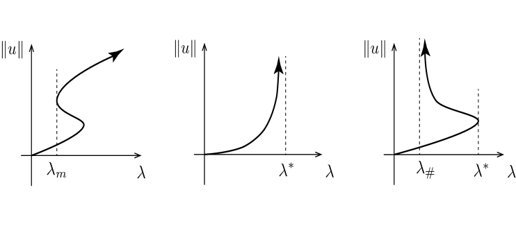
Figure 1. Schematic of some typical situations dealt with Theorem 3.2. The left panel corresponds to case (i), the right panel corresponds to case (ii), and the middle panel corresponds to case (iii). In each case, either a multiple-point or a new fold-point can be created (locally) by arbitrary small perturbations of the nonlinearity $g$ in (3.1), as described in Theorem 3.2. The appearance of such singular points implies a topological instability —  in the sense of Definition 2.5 —  of the one-parameter family of semigroups associated with the corresponding family of parabolic problems.

The qualitative changes described at the end of the previous section may be therefore interpreted in that terms; see also [MN07, Fig.  1]. Singularity theory is a natural framework to study the effects on the bifurcation diagram of small perturbations or imperfections to a given static model [GS79, GS85]. In that spirit, geometric connections between a double turning point and a cusp point have been discussed for certain nonlinear elliptic problems in e.g. [BCT88a, BF82, MS80, SW82]. However, a general understanding of the effects of arbitrary perturbations on bifurcation diagrams remains a challenging problem, especially when the perturbations are not necessarily smooth; see however [Dan08, Hen05] for related issues.

Complementarily, it is tempting to describe the aforementioned qualitative changes in terms of structural instability such as encountered in classical dynamical systems theory [AM87, Arn83, Sma67]. Nevertheless, as will be explained in Section 2.3, such topological ideas have to be recast into a formalism which takes into account the functional setting in which the parabolic and corresponding elliptic problems are considered; see Definitions 2.1, 2.2 and 2.5 below.

This formalism will turn out to be particularly suitable for problems such as arising in combustion theory or chemical kinetics [F-K69] for which the associated semigroups are not necessarily dissipative while still exhibiting finitely many local attractors which attract the trajectories that remain bounded. To better appreciate this distinction with the standard theory, we recall briefly below the notion of structural stability such as encountered for dissipative infinite-dimensional systems.

Originally formulated for finite-dimensional dynamical systems [AP37], the notion of structural stability has been extended to infinite-dimensional dynamical systems, mainly dissipative. As a rule of thumb for such dynamical systems, one investigates structural stability of the semiflow restricted to a compact invariant set, usually the global attractor, rather than the flow in the original state space [HMO02, Definition 1.0.1]; an exception can be found in e.g.  [Lu94] where the author considered the semiflow in a neighborhood of the global attractor.

In the context of reaction-diffusion problems, the problem of structural stability is concerned with,

(2.4) $$\left\{\begin{array}[]{l}\partial_{t}u-\Delta u=g(u),\;\textrm{ in }\Omega,\;\;g\in C^{1}(\mathbb{R},\mathbb{R}),\\ \hskip 18.50008ptu|_{\partial{\Omega}}=0,\end{array}\right.$$

that is assumed to generate a semigroup $\{S(t)\}_{t\geq 0}$ for which a global attractor $\mathcal{A}_{g}$, in some Banach space $X$, exists [BP97, FR99, HMO02, Lu94].

Within this context, the structural stability problem may be formulated as the existence problem of an homeomorphism $H:\mathcal{A}_{g}\rightarrow\mathcal{A}_{\widehat{g}}$ for arbitrarily small perturbations $\widehat{g}$ of $g$ in some topology $\mathcal{T}$ on $C^{1}(\mathbb{R},\mathbb{R})$, that aims to satisfy the following properties

(2.5a) $$\mathcal{A}_{\widehat{g}}\mbox{ is a global attractor in }X\mbox{ of }\{\widehat{S}(t)\}_{t\in\mathbb{R}^{+}},\mbox{ and }$$

(2.5b) $$\forall\;t\in\mathbb{R},\;\forall\;\phi\in\mathcal{A}_{g},\;H(S(t)\phi)=\widehat{S}(t)H(\phi),$$

where $\{\widehat{S}(t)\}_{t\in\geq 0}$ denotes the semigroup generated by

$$u_{t}-\Delta u=\widehat{g}(u),\;u|_{\partial\Omega}=0.$$

The topology $\mathcal{T}$ may be chosen to be for instance the compact-open topology or the finer topology of Whitney. Note that in (2.5b), the restriction of the dynamics to the global attractor, allows for backward trajectories onto the global attractor giving rise to genuine flows onto the global attractor; see e.g. [FR99, Rob01].

Once a parabolic equation generates a semigroup, a necessary condition to exhibit a global attractor (in some Banach $X$) is to satisfy a dissipation property, i.e. to verify the existence of an absorbing ball in $X$ for this semigroup; see e.g. [MWZ02, Theorem 3.8].

However, such a working assumption may be viewed as too restrictive. As mentioned above, in many applications although blow-up in finite or infinite time may occur for certain trajectories, many other trajectories are typically attracted by local attractors depending on the “energy” of their initial data; see [BE89, Ben10, CH98, F-K69, Fil05, QS07].

Furthermore given a parameterized family of elliptic problems subject to perturbations, if one wants to translate a qualitative change of its bifurcation diagram into dynamical terms for the corresponding parabolic problems, one has to take into account the possible discrepancies of regularity between the (weak) steady state solutions and the semigroup equilibria. The next section introduces a framework to deal with these issues.

2.3. Topological robustness for general families of semilinear parabolic problems

To deal with the problem of topological equivalence between families of semigroups which may exhibit non-global dissipative properties, we start by introducing several intermediate concepts allowing for taking into account the possible discrepancies between the functional settings in which the parabolic and corresponding elliptic problems are well-posed; see Definitions 2.1, 2.2 and 2.5 below. Throughout this section we illustrate these concepts on some standard semilinear parabolic and elliptic problems.

Let us first consider a parameterized family $\mathfrak{F}_{f}:=\{f_{\lambda}\}_{\lambda\in\Lambda}$ of functions $I\rightarrow\mathbb{R}$, where $\Lambda$ is a metric space, and $I$ is an unbounded interval of $\mathbb{R}$. We are concerned with the associated parameterized family of semilinear parabolic problems,

($$\mathcal{P}_{f_{\lambda}} \left\{\begin{array}[]{l}\partial_{t}u-\Delta u=f_{\lambda}(u),\quad\mbox{ in }\;\Omega,\\ \;\;\;\;\;\;u=0,\quad\quad\qquad\mbox{ on }\;\partial\Omega,\end{array}\right.$$)

where $\Omega$ is an open bounded subset of $\mathbb{R}^{d}$, with additional regularity assumptions on its boundary and $f_{\lambda}$ when needed.

In general, these problems may generate a family of semigroups acting on a functional space $X$ that does not necessarily agree with the functional space $Y$ on which the (weak) solutions of

(2.6) $$\left\{\begin{array}[]{l}-\Delta u=f_{\lambda}(u),\qquad\mbox{ in }\;\Omega,\\ \;\;\;\;\;\;u=0,\quad\quad\qquad\mbox{ on }\;\partial\Omega,\end{array}\right.$$

exist. As shown in Example 2.1 below, such situations arise when weak solutions to (2.6) do not necessarily correspond to equilibria of the semigroup associated with ($\mathcal{P}_{f_{\lambda}}$). These considerations lead us naturally to introduce the following definition that makes precise the class of problems ($\mathcal{P}_{f_{\lambda}}$) we consider hereafter.

Definition 2.1.

Let $\Lambda$ be a metric space. Let $Y$ be a Banach space and $\Omega$ be an open bounded subset of $\mathbb{R}^{d}$, such that (2.6) makes sense in $Y$.

Given a Banach space $X$, a family of functions, $\mathfrak{F}_{f}:=\{f_{\lambda}\}_{\lambda\in\Lambda^{*}}$, is be said to be $(X;Y)$-compatible relatively to $\Lambda^{*}\subset\Lambda$ and $\Omega$, if there exists a subset $\Lambda^{*}\subset\Lambda$, such that for all $\lambda\in\Lambda^{*}$ the following properties are satisfied:

• There exists a nonempty subset $D(f_{\lambda})\subset X$ such that ($\mathcal{P}_{f_{\lambda}}$) generates a semigroup $\{S_{\lambda}(t)\}_{t\geq 0}$ on $D(f_{\lambda})$.

• The set $\mathcal{V}_{f_{\lambda}}:=\{u\in Y\;:\;-\Delta u=f_{\lambda}(u),\;u|_{\partial\Omega}=0\}$ is non-empty.

• The set $\mathcal{E}_{f_{\lambda}}$ of equilibria of $\{S_{\lambda}(t)\}_{t\geq 0}$, satisfies

  $$\mathcal{E}_{f_{\lambda}}:=\{\phi\in D(f_{\lambda})\;:\;S_{\lambda}(t)\phi=\phi,\;\forall\;t\geq 0\}=\mathcal{V}_{f_{\lambda}}.$$

If instead of (iii),

(2.7) $$\overline{\mathcal{E}_{f_{\lambda}}}^{X}=\mathcal{V}_{f_{\lambda}},\mbox{ with }\mathcal{E}_{f_{\lambda}}\varsubsetneq\ \mathcal{V}_{f_{\lambda}},$$

then $\mathfrak{F}_{f}$ is be said to be weakly $(X;Y)$-compatible relatively to $\Lambda^{*}\subset\Lambda$ and $\Omega$.

Remark 2.1.

When the domain $\Omega$ is clear from the context, we simply say that a family of functions is $(X;Y)$-compatible without referring to $\Omega$. We will also often say that the family of elliptic problems (2.6) is $(X;Y)$-compatible, when the corresponding family of function $\{f_{\lambda}\}$ is $(X;Y)$-compatible.

We first provide an example of a family of superlinear elliptic problems that is not $(C^{1}(\overline{\Omega});H_{0}^{1}(\Omega))$-compatible, but only weakly $(C^{1}(\overline{\Omega});H_{0}^{1}(\Omega))$-compatible.

Example 2.1.

It may happen that $\mathcal{E}_{f_{\lambda}}\neq\mathcal{V}_{f_{\lambda}}$ for some $\lambda\in\Lambda^{*}$. The Gelfand problem [Gel63, Fuj69],

(2.8) $$-\Delta u=\lambda e^{u},\;u|_{\partial B_{1}(0)}=0,$$

where $B_{1}(0)$ is a unit ball of $\mathbb{R}^{d}$ with $3\leq d\leq 9$, is an illustrative example of such a distinction that may arise between the set of equilibrium points and the set of steady states, depending on the functional setting adopted.

In that respect, let us first recall that for $Y=H^{1}_{0}(B_{1}(0))$ there exists $\lambda^{*}>0$ such that for $\lambda>\lambda^{*}$ there is no solution to (2.8), even in a very weak sense [BCMR96], whereas for $\lambda\in[0,\lambda^{*}]$ there exists at least a solution (in $Y$) so that $\mathcal{V}_{f}\neq\emptyset$; see [BV97] and Proposition 3.1 below.

In what follows we denote by $A_{p}$ the (closed) Laplace operator considered as an unbounded operator on $L^{p}(B_{1}(0))$ under Dirichlet conditons, with domain

$$D(A_{p})=W^{2,p}(B_{1}(0))\cap W_{0}^{1,p}(B_{1}(0));$$

see [Paz83, Sect. 7.3].

Let us now take $\Lambda^{*}$ to be $[0,\lambda^{*}]$ and let us choose $X$ to be the following subspace constituted by radial functions

(2.9) $$X:=\{\varphi(r)\;:\;\varphi\in D(A_{p}^{\beta})\},$$

where $D(A_{p}^{\beta})$ denotes the domain of $A_{p}^{\beta}$, the fractional power of $A_{p}$, where $0<\beta\leq 1$; see e.g.  [Paz83, Sect. 2.6] and [Hen81, Sect. 1.4].

For $p>d$ and $1>\beta>(d+p)/(2p)$, it is known that $D(A_{p}^{\beta})$ is compactly embedded in $C^{1}(\overline{B_{1}(0)})$ [Hen81, Thm. 1.6.1], and thus $X\hookrightarrow C^{1}(\overline{B_{1}(0)})$. Then for any $\lambda\in[0,\lambda^{*}]$ and for such a choice of $p$ and $\beta$, the parabolic problem $\eqref{Eq_family-parab}$ is well posed in $X$ with $f_{\lambda}(x)=\lambda\exp(x)$, see [CH98, SY02, Lun95].

As a consequence, by introducing

(2.10) $$D(f_{\lambda}):=\{u_{0}\in X\;:\;u_{\lambda}(t;u_{0})\mbox{ exists for all }t>0,\mbox{ and }\underset{t>0}{\sup}\;\|A_{p}^{\beta}u_{\lambda}(t;u_{0})\|_{p}<\infty\},$$

a nonlinear semigroup $\{S_{\lambda}(t)\}_{t\geq 0}$ on $D(f_{\lambda})$ can be defined as follows

(2.11) $$S_{\lambda}(t)u_{0}:=u_{\lambda}(t;u_{0}),\;t\geq 0,\;u_{0}\in D(f_{\lambda}),$$

where $u_{\lambda}(t;u_{0})$ denotes the solution of ($\mathcal{P}_{f_{\lambda}}$) emanating from $u_{0}$ at $t=0$.

However the property (iii) of Definition 2.1 is not verified here. Indeed, for $\lambda=\lambda^{\sharp}=2(d-2)\in(0,\lambda^{*})$ there exists in $H_{0}^{1}(B_{1}(0))$ an unbounded solution of the Gelfand problem (2.8) —  in the weak sense of [BCMR96] —  given by

$$u_{\lambda^{\sharp}}(x):=-2\log\|x\|,$$

see [BV97].

This solution does not belong to $D(f_{\lambda})\subset X\subset C^{1}(\overline{B_{1}(0)})$ and in particular to $\mathcal{E}_{f_{\lambda^{\sharp}}}$, the set of equilibria of $S_{\lambda}(t)$ in $D(f_{\lambda})$ given by (2.10).

Therefore the family

(2.12) $$\mathfrak{F}_{\mbox{exp}}=\{x\mapsto\lambda e^{x},x\geq 0,\;\lambda\in[0,\lambda^{*}]\},$$

is not $(C^{1}(\overline{B_{1}(0)});H_{0}^{1}(B_{1}(0)))$-compatible relatively to $[0,\lambda^{*}]$ where $B_{1}(0)$ is the unit open ball of $\mathbb{R}^{d}$, for $3\leq d\leq 9$.

Nevertheless this family is weakly $(C^{1}(\overline{B_{1}(0)});H_{0}^{1}(B_{1}(0)))$-compatible relatively to $[0,\lambda^{*}]$, in the sense of Definition 2.1. This property results from the fact that the singular steady state $u_{\lambda^{\sharp}}$ can be approximated by a sequence of equilibria in $X$ for the relevant topology [BV97, JL73], so that in particular condition (2.7) is verified.

The following proposition identifies a broad class of families of sublinear elliptic problems which are $(C_{0}^{0,2\alpha}([0,1]);C^{2}([0,1]))$-compatible for $\alpha\in(\frac{1}{2},1)$.

Proposition 2.1.

Let us consider a function $f:[0,\infty)\rightarrow(0,\infty)$ that satisfies the following conditions:

• $f$ is locally Lipschitz, and such that for all $\sigma>0$, the following properties hold:

  • $f\in C^{\theta}([0,\sigma])$, for some $\theta\in(0,1)$ (independent of $\sigma$), and

  • $\exists\;\omega(\sigma)>0$ such that

    $$f(y)-f(x)>-\omega(\sigma)(y-x),\;0\leq x<y\leq\sigma.$$

• $x\mapsto f(x)/x$ is strictly decreasing on $(0,\infty)$.

• $\underset{x\rightarrow\infty}{\lim}(f(x)/x)=b,$ with $b\geq 0$.

Let us define $a=\underset{x\rightarrow 0}{\lim}(f(x)/x)$, and $\Lambda^{*}:=(\frac{\lambda_{1}}{a},\frac{\lambda_{1}}{b}).$

If $a<\infty$, then $\mathfrak{F}_{f}=\{\lambda f\}_{\lambda\in\Lambda^{*}}$ is $(C_{0}^{0,2\alpha}([0,1]);C^{2}([0,1]))$-compatible relatively to $\Lambda^{*}$, for $\alpha\in(\frac{1}{2},1)$.

Proof.

This proposition is a direct consequence of the theory of analytic semigroups [Lun95, Paz83, SY02, Tai95] and the theory of sublinear elliptic equations [BO86].

Consider $\Lambda=[0,\infty)$, and $f_{\lambda}=\lambda f$, for $\lambda\in[0,\infty)$. Then from [Tai98, Theorem 5] which generalizes the “classical” result of [BO86, Theorem 1], we have that

$$-\partial_{xx}^{2}u=\lambda f(u),\;u(0)=u(1)=0,$$

has a unique solution $u\in C^{2}([0,1)])$ if and only if

(2.13) $$\frac{\lambda_{1}}{a}<\lambda<\frac{\lambda_{1}}{b},$$

where $\lambda_{1}$ is the first eigenvalue of $-\partial_{xx}^{2}$ with Dirichlet condition.

Let us consider $\Lambda^{*}:=(\frac{\lambda_{1}}{a},\frac{\lambda_{1}}{b}).$ The realization of the Laplace operator $A=-\partial_{xx}^{2}$ in $X=C([0,1])$ with domain,

(2.14) $$D(A)=C^{0,2\alpha}_{0}([0,1]):=\{u\in C^{0,2\alpha}([0,1])\;:\;u(0)=u(1)=0\},$$

is sectorial for $\alpha\in(\frac{1}{2},1)$, and therefore generates an analytic semigroup on $X$; see [Lun95].

The theory of analytic semigroups shows that under the aforementioned assumptions on $f$, for every $u_{0}\in C_{0}^{0,2\alpha}([0,1])$, there exists a unique solution $u_{\lambda}\in C^{1}((0,\tau_{\lambda}(u_{0}));C^{2}([0,1]))$ of ($\mathcal{P}_{f_{\lambda}}$) defined on a maximal interval $[0,\tau_{\lambda}(u_{0})),$ with $\tau_{\lambda}(u_{0})>0$ (and $f_{\lambda}=\lambda f$); see e.g. [LLMP05, Proposition 6.3.8]. Since our assumptions on $f$ imply that there exists $C>0$ such that $0\leq f(x)\leq C(1+x)$ for all $x\geq 0$, from e.g. [LLMP05, Proposition 6.3.5] we can deduce that $\tau_{\lambda}(u_{0})=\infty.$

Let us introduce now,

(2.15) $$D(f_{\lambda}):=\{u_{0}\in C_{0}^{0,2\alpha}([0,1])\;:\;\underset{t>0}{\sup}\;\|u_{\lambda}(t;u_{0})\|_{C^{2}([0,1])}<\infty\},$$

then $S_{\lambda}(t):D(f_{\lambda})\rightarrow D(f_{\lambda})$, defined by $S_{\lambda}(t)u_{0}=u_{\lambda}(t;u_{0})$ is well defined for all $t\geq 0$, and for all $u_{0}\in D(f_{\lambda})$. From the existence and uniqueness properties of the solutions, we deduce that $\{S_{\lambda}(t)\}_{t\geq 0}$ is a (nonlinear) semigroup on $D(f_{\lambda}),$ in the sense that $S_{\lambda}(t)\in C(D(f_{\lambda}),D(f_{\lambda})),$

(2.16) $$S_{\lambda}(t+s)=S_{\lambda}(t)\circ S_{\lambda}(s),\;\;\forall\,t,s\geq 0,$$

and that each trajectory $t\mapsto S_{\lambda}(t)u_{0}$ is continuous in $D(f_{\lambda})$.

It is now easy to verify from what precedes that (ii) and (iii) of Definition 2.1 are satisfied. We have thus proved that $\mathfrak{F}_{f}=\{\lambda f\}_{\lambda\in\Lambda^{*}}$ is $(C_{0}^{0,2\alpha}([0,1]);C^{2}([0,1]))$-compatible relatively to $\Lambda^{*}$, for $\alpha\in(\frac{1}{2},1)$. ∎

Remark 2.2.

Let us remark that if we assume furthermore that $\lambda b>\lambda_{1}^{-1}$, it can be then proved that there exists at least one solution $u$ to $\eqref{Eq_family-parab}$ emanating from some $u_{0}\in C_{0}^{0,2\alpha}([0,1])$ for which $u$ does not remain in any bounded set for all time [Ben10, Lemma 10.1, Remark 10.2]. Such a trajectory becomes unbounded in infinite time. It is the possible occurrence of such a phenomenon that motivated to include a boundedness requirement in the definition of $D(f_{\lambda})$ in (2.15).

Example 2.2.

Let $g_{\varepsilon}(x)=\exp(x/(1+\varepsilon x))$. A simple calculation shows that for $x\neq 0$,

$$\Big{(}\frac{g_{\varepsilon}(x)}{x}\Big{)}^{\prime}=-\frac{\exp(\frac{x}{1+\varepsilon x})}{x^{2}(1+\varepsilon x)^{2}}(\varepsilon^{2}x^{2}+(2\varepsilon-1)x+1),$$

which implies in particular that $g_{\varepsilon}(x)/x$ is strictly decreasing for all $x>0$ if $\varepsilon>1/4$. Note also that Condition (G₁) of Proposition 2.1 is satisfied, and that $b=0$ and $a=\infty$ in this case.

A semigroup can still be defined (for each $\lambda\in(0,\infty)$) on the subset $D(\lambda g_{\varepsilon})$ such as given in (2.15) with $f_{\lambda}=\lambda g_{\varepsilon}.$ From the proof of Proposition 2.1, it is then easy to deduce that the family $\{\lambda g_{\varepsilon}\}_{\lambda\in(0,\infty)}$ is in fact $(C_{0}^{0,2\alpha}([0,1]);C^{2}([0,1]))$-compatible relatively to $(0,\infty)$, for $\alpha\in(\frac{1}{2},1)$ and $\varepsilon>1/4.$

Hereafter, $X$ and $Y$ are two Banach spaces with respective norms denoted by $\|\cdot\|_{X}$ and $\|\cdot\|_{Y}$; and $\Omega$ denotes an open bounded subset of $\mathbb{R}^{d}$, such that the following elliptic problem

(2.17) $$-\Delta u =f_{\lambda}(u),\;\mbox{ in }\Omega,$$

$$u =0,\qquad\mbox{ on }\partial\Omega,$$

makes sense in $Y$. We introduce below a concept of topological equivalence between families of semilinear parabolic problems for $(X;Y)$-compatible families of nonlinearities.

Definition 2.2.

Let $\Lambda$ be a metric space and $I$ be an unbounded interval of $\mathbb{R}$. Let $\mathcal{N}(I,\mathbb{R})$ be a set of functions from $I$ to $\mathbb{R}$. Consider two families $\{f_{\lambda}\}_{\lambda\in\Lambda^{*}}$ and $\{\widehat{f}_{\lambda}\}_{\lambda\in\widehat{\Lambda}^{*}}$ of $\mathcal{N}(I,\mathbb{R})$, which are both $(X;Y)$-compatible relatively to $\Lambda^{*}$ and $\widehat{\Lambda}^{*}$ respectively.

For each $\lambda\in\Lambda^{*}$ and $\lambda\in\widehat{\Lambda}^{*}$, one denotes by $\{S_{\lambda}(t)\}_{t\geq 0}$ and $\{\widehat{S}_{\lambda}(t)\}_{t\geq 0}$, the semigroups acting on $D(f_{\lambda})$ and $D(\widehat{f}_{\lambda})$, and associated with ($\mathcal{P}_{f_{\lambda}}$) and (${\color[rgb]{0,0,1}\mathcal{P}_{\widehat{f}_{\lambda}}}$), respectively. One denotes finally by $\mathfrak{S}_{f}$ and by $\mathfrak{S}_{\widehat{f}}$, the respective family of such semigroups.

Then $\mathfrak{S}_{f}$ and $\mathfrak{S}_{\widehat{f}}$ are called topologically equivalent if there exists an homeomorphism

$$H:\Lambda\times\underset{\lambda\in\Lambda^{*}}{\bigcup}D(f_{\lambda})\rightarrow\Lambda\times\underset{\lambda\in\widehat{\Lambda}^{*}}{\bigcup}D(\widehat{f}_{\lambda}),$$

such that $H(\lambda,u)=(p(\lambda),H_{\lambda}(u))$ where $p$ and $H_{\lambda}$ satisfy the following two conditions:

• $p$ is an homeomorphism from $\Lambda^{*}$ to $\widehat{\Lambda}^{*}$,

• for all $\lambda\in\Lambda^{*}$, $H_{\lambda}$ is an homeomorphism from $D(f_{\lambda})$ to $D(\widehat{f}_{p(\lambda)})$, such that,

  (2.18) $$\forall\;\lambda\in\Lambda^{*},\;\forall\;u_{0}\;\in D(f_{\lambda}),\;\forall\;t>0,\;H_{\lambda}(S_{\lambda}(t)u_{0})=\widehat{S}_{p(\lambda)}(t)H_{\lambda}(u_{0}).$$

In case of such an equivalence, the families of problems $\{\eqref{Eq_family-parab}\}_{\lambda\in\Lambda^{*}}$ and $\{({\color[rgb]{0,0,1}\mathcal{P}_{\widehat{f}_{\lambda}}})\}_{\lambda\in\widehat{\Lambda}^{*}}$ is also referred to as topologically equivalent.

Remark 2.3.

Note that the relation of topological equivalence given by (2.18) may be relaxed as follows,

(2.19) $$\forall\;\lambda\in\Lambda,\;\forall\;u_{0}\;\in D(f_{\lambda}),\;H_{\lambda}(S_{\lambda}(t)u_{0})=\widehat{S}_{p(\lambda)}(\gamma(t,u_{0}))H_{\lambda}(u_{0}),$$

where $\gamma:[0,\infty)\times D(f_{\lambda})\rightarrow[0,\infty)$ is an increasing and continuous function of the first variable.

The equivalence relation (2.19) is known as the topological orbital equivalence. It allows, in particular, for systems presenting periodic orbits of different periods, to be equivalent.

In contrast, the topological equivalence relation (2.18) excludes this possibility, which might be viewed as too restrictive for general semigroups, at a first glance. However, for semigroups generated by semilinear parabolic equations over bounded domain, due to their gradient structure [CH98, Sect. 9.4], this problem of modulii does not occur since the $\omega$-limit set of each semigroup is typically included into the set of its equilibria [CH98, Thm. 9.2.7].

Definition 2.3.

Let $\mathfrak{S}_{f}$ be a family of semigroups as defined in Definition 2.2. Let $\mathcal{E}_{f}$ be the corresponding family of equilibria, in the sense that,

(2.20) $$\mathcal{E}_{f}:=\{(\lambda,\phi_{\lambda})\in\Lambda\times D(f_{\lambda})\;:\;S_{\lambda}(t)\phi_{\lambda}=\phi_{\lambda},\;\forall\;t\in(0,\infty)\}.$$

Assume that $\Lambda$ is an unbounded interval of $\mathbb{R}$. A fold-point on $\mathcal{E}_{f}$ is a point $(\lambda^{*},u^{*})\in\mathcal{E}_{f}$, such that there exists a local continuous map

$$\mu:s\in(-\varepsilon,\varepsilon)\mapsto(\lambda(s),u(s))\mbox{ for some }\varepsilon>0,$$

verifying the following properties:

• For all $s\in(-\varepsilon,\varepsilon)$, one has $(\lambda(s),u(s))\in\mathcal{E}_{f}$, with $(\lambda(0),u(0))=(\lambda^{*},u^{*})$.

• The map $s\mapsto\lambda(s)$ has a unique extremum on $(-\varepsilon,\varepsilon)$ attained at $s=0$.

• There exists $r^{*}>0$ such that for all $0<r<r^{*},$ the set

  $$\partial\mathfrak{B}((\lambda^{*},u^{*});r)\bigcap\{\mu(s),\;s\in(-\varepsilon,\varepsilon)\},$$

  has cardinal two; where

  (2.21) $$\mathfrak{B}((\lambda^{*},u^{*});r):=\{(\lambda,u)\in\mathbb{R}\times D(f_{\lambda}),\;:\;|\lambda-\lambda^{*}|+{\color[rgb]{0,0,0}\|u-u^{*}\|_{X}}<r\}.$$

Definition 2.4.

Let $\mathfrak{S}_{f}$ be a family of semigroups as defined in Definition 2.2. Let $\mathcal{E}_{f}$ be the corresponding family of equilibria given by (2.20). Assume that $\Lambda$ is an unbounded interval of $\mathbb{R}$. Let $n$ be an integer such that $n\geq 3$. A multiple-point with $n$ branches on $\mathcal{E}_{f}$ is a point $(\lambda^{*},u^{*})\in\mathcal{E}_{f}$, such that there exists at most $n$ local continuous map

$$\mu_{i}:s\in(-\varepsilon_{i},\varepsilon_{i})\mapsto(\lambda_{i}(s),u_{i}(s))\mbox{ for some }\varepsilon_{i}>0,\;i\in\{1,...,n\},$$

verifying the following properties:

• $\mu_{i}\neq\mu_{j}$ for all $i\neq j$.

• For all $i\in\{1,...,n\}$, and for all $s\in(-\varepsilon_{i},\varepsilon_{i})$, one has $(\lambda_{i}(s),u_{i}(s))\in\mathcal{E}_{f}$, with $(\lambda_{i}(0),u_{i}(0))=(\lambda^{*},u^{*})$.

• There exists $r^{*}>0$ such that for all $0<r<r^{*},$ the set

  $$\partial\mathfrak{B}((\lambda^{*},u^{*});r)\bigcap\underset{i\in\{1,...,n\}}{\bigcup}\{\mu_{i}(s),\;s\in(-\varepsilon_{i},\varepsilon_{i})\},$$

  has cardinal $n$, where $\mathfrak{B}((\lambda^{*},u^{*});r)$ is as given in (2.21).

Remark 2.4.

The terminologies of Definitions 2.3 and 2.4 regarding the singular points of $\mathcal{E}_{f}$ will be also adopted, when they apply, for the singular points of the solution set associated with the family of elliptic problems (2.6).

Based on these definitions, simple criteria of non-topological equivalence between two families of semigroups can be then formulated. The proposition below whose proof is left to the reader’s discretion, summarizes these criteria.

Proposition 2.2.

Assume $\Lambda$ is an unbounded interval of $\mathbb{R}$. Let $\mathfrak{S}_{f}$ and $\mathfrak{S}_{\widehat{f}}$ be two families of semigroups as defined in Definition 2.2. Let $\mathcal{E}_{f}$ and $\mathcal{E}_{\widehat{f}}$ be the corresponding families of equilibria. Then $\mathfrak{S}_{f}$ and $\mathfrak{S}_{\widehat{f}}$ are not topologically equivalent if one of the following conditions are fulfilled.

• $\mathcal{E}_{f}$ is constituted by a single unbounded continuum in $\Lambda\times X$, and $\mathcal{E}_{\widehat{f}}$ is the union of at least two disjoint unbounded continua in $\Lambda\times X$.

• $\mathcal{E}_{f}$ and $\mathcal{E}_{\widehat{f}}$ are each constituted by a single continuum, and the set of fold-points of $\mathcal{E}_{f}$ and $\mathcal{E}_{\widehat{f}}$ are not in one-to-one correspondence.

• $\mathcal{E}_{f}$ and $\mathcal{E}_{\widehat{f}}$ are each constituted by a single continuum, and there exists an integer $n\geq 3$ such that the set of multiple-points with $n$ branches of $\mathcal{E}_{f}$ and $\mathcal{E}_{\widehat{f}}$ are not in one-to-one correspondence.

We are now in position to formulate our notion of topological robustness to small perturbations for family of semigroups which may exhibit a non-global dissipative behavior. In that respect, a first requirement that is needed in practice concerns the stability of the $(X;Y)$-compatibility of the underlying family of nonlinearities, in order to stay, loosely speaking, within the same functional setting when a perturbation is applied. This is formulated in the following definition.

Definition 2.5.

Let $\Lambda$ be a metric space and $I$ be an unbounded interval of $\mathbb{R}$. Let $\mathcal{N}(I,\mathbb{R})$ be a set of functions from the interval $I$ to $\mathbb{R}$ endowed with a topology $\mathcal{T}$. Consider a family $\mathfrak{F}_{f}=\{f_{\lambda}\}_{\lambda\in\Lambda^{*}}$ of $\mathcal{N}(I,\mathbb{R})$ which is $(X;Y)$-compatible relatively to $\Lambda^{*}\subset\Lambda$.

Let $\mathcal{P}$ be an open subset of $\mathcal{N}(I,\mathbb{R})$ for the $\mathcal{T}$-topology. The family $\mathfrak{F}_{f}$ is said to be $\mathcal{T}$-stable with respect to perturbations in $\mathcal{P}$, if there exist an interval $\Lambda^{\prime}\supseteq\Lambda^{\ast}$ and a neighborhood $\mathcal{U}^{\prime}_{\lambda}$ of $f_{\lambda}$ in the $\mathcal{T}$-topology such that for any neighborhood $\mathcal{U}_{\lambda}\subset\mathcal{U}^{\prime}_{\lambda}$, we have

$$\Big{(}\;\widehat{f}_{\lambda}\in\mathcal{U}_{\lambda}\mbox{ and }\widehat{f}_{\lambda}-f_{\lambda}\in\mathcal{P},\,\lambda\in\Lambda^{\prime}\Big{)}\Rightarrow\Big{(}\{\widehat{f}_{\lambda}\}_{\lambda\in\Lambda^{\prime}}\mbox{ is }(X;Y)\mbox{-compatible relatively to }\Lambda^{\prime}\Big{)}.$$

Example 2.3.

Let us consider $\mathcal{N}((0,\infty),\mathbb{R})$ endowed with the $C^{0}$-topology $\mathcal{T}$ of uniform convergence over compact sets. Let us consider $f_{\lambda}=\lambda g_{\varepsilon}$, with $g_{\varepsilon}(x)=\exp(x/(1+\varepsilon x))$, and $\lambda\in\Lambda=\Lambda^{\ast}=(0,\infty)$.

We saw in Example 2.2 that the corresponding family, $\mathfrak{F}=\{f_{\lambda}\}_{\lambda\in\Lambda}$, is $(C_{0}^{0,2\alpha}([0,1]);C^{2}([0,1]))$-compatible relatively to $\Lambda$ for $\alpha\in(\frac{1}{2},1)$ and $\varepsilon>1/4$.

Let $\mathcal{P}$ be the set of functions $\varphi$ with compact support such that $\widehat{g}:=g_{\varepsilon}+\varphi$ is locally Liptchitz and satisfies the rest of assumptions of Proposition 2.1. This set is non empty. Indeed, if we consider $0<m<M$, $r=\displaystyle\lambda\frac{g_{\varepsilon}(M)-g_{\varepsilon}(m)}{M-m}$, and $\varphi$ given by

(2.22) $$\varphi(x) =r(x-m)+\lambda(g_{\varepsilon}(m)-g_{\varepsilon}(x)),\mbox{ for }x\in(m,M),$$

$$\varphi(x) =0,\mbox{ otherwise},$$

then the function $g_{\varepsilon}+\varphi$ satisfies the desired assumptions. Furthermore this perturbation can be made as close as desired to $g_{\varepsilon}$ (in the aforementioned $C^{0}$-topology $\mathcal{T}$) by reducing the size of the interval $(m,M)$, accordingly.

Now since the assumptions of Proposition 2.1 are satisfied for any $g_{\varepsilon}+\varphi$ with $\varphi\in\mathcal{P}$, we conclude that $\mathfrak{F}^{\prime}=\{\lambda(g_{\varepsilon}+\varphi)\}_{\lambda\in\Lambda}$ is $(C_{0}^{0,2\alpha}([0,1]);C^{2}([0,1]))$-compatible relatively to $\Lambda^{\prime}=(0,\infty)$ for $\alpha\in(\frac{1}{2},1)$. In other words, $\mathfrak{F}$ is $\mathcal{T}$-stable with respect to perturbations in $\mathcal{P}$, for $\varepsilon>1/4$.

Note that in the proof of Corollary 3.1 below, the family $\mathfrak{F}$ is shown to be $\mathcal{T}$-stable for another class of perturbations than considered here, emphasizing thus that a given family can be $\mathcal{T}$-stable with respect to different type of perturbations.

The desired notion of topological robustness to small perturbations and the related notion of topological instability can be then formulated as follows.

Definition 2.6.

Let us consider the setting of Definition 2.5. For each $\lambda$, one denotes by $\{S_{\lambda}(t)\}_{t\geq 0}$ (resp. $\{\widehat{S}_{\lambda}(t)\}_{t\geq 0}$) the semigroup acting on $D(f_{\lambda})$ (resp. $D(\widehat{f}_{\lambda})$), given a function $f_{\lambda}$ (resp. $\widehat{f}_{\lambda}$). One denotes also by $\mathfrak{S}_{f}$ and $\widehat{\mathfrak{S}}_{f}$ the corresponding family of semigroups generated respectively by ($\mathcal{P}_{f_{\lambda}}$) and (${\color[rgb]{0,0,1}\mathcal{P}_{\widehat{f}_{\lambda}}}$).

In case where $\mathfrak{F}_{f}$ is $\mathcal{T}$-stable, we say furthermore that $\mathfrak{S}_{f}$ is $\mathcal{T}$-topologically robust in $X$ with respect to perturbations in $\mathcal{P}$ for the $\mathcal{T}$-topology, if there exists a neighborhood $\mathcal{U}^{\prime}_{\lambda}$ of $f_{\lambda}$ such that for any neighborhood $\mathcal{U}_{\lambda}\subset\mathcal{U}^{\prime}_{\lambda}$, we have over some interval $\Lambda^{\prime}\supseteq\Lambda^{\ast}$,

(2.23) $$\Big{(}\widehat{f}_{\lambda}\in\mathcal{U}_{\lambda}\mbox{ and }\widehat{f}_{\lambda}-f_{\lambda}\in\mathcal{P}\Big{)}\Rightarrow\Big{(}\mathfrak{S}_{\widehat{f}}\sim\mathfrak{S}_{f}\Big{)},$$

where $\mathfrak{S}_{\widehat{f}}\sim\mathfrak{S}_{f}$ means that $\mathfrak{S}_{\widehat{f}}$ and $\mathfrak{S}_{\widehat{f}}$ are topologically equivalent in the sense of Definition 2.2.

Given a $\mathcal{T}$-stable family $\mathfrak{F}_{f}$, in case of violation of (2.23), then $\mathfrak{S}_{f}$ is said to be topologically unstable with respect to small perturbations in $\mathcal{P}$ for the $\mathcal{T}$-topology.

3. Topologically unstable families of semilinear parabolic problems: Main result

We are now in position to formulate the main result of this article, Theorem 3.2, regarding the topological instability of a broad class of semilinear parabolic problems. As the proof will show, the abstract framework introduced in the previous section allows us to relate these instabilities to local deformations—of the $\lambda$-bifurcation diagram of the corresponding elliptic problems—which occur when appropriate small perturbations are applied to the nonlinear term.

Figure 1 below depicts some typical bifurcation diagrams for which Theorem 3.2 predicts the apparition of either a multiple-point or a new fold-point on it when the nonlinearity is appropriately perturbed. It is worth mentioning that the parabolic problems corresponding to such bifurcation diagrams allow for a possible mixed dynamical behavior composed by finitely many local attractors and unbounded trajectories, justifying the revision of the standard notion of structural stability such as proposed in Section 2.3.

To prepare the proof of Theorem 3.2, one first recall some standard results regarding the solution set of,

(3.1) $$\left\{\begin{array}[]{l}-\Delta u=\lambda g(u),\;\textrm{ in }\Omega,\;\lambda\geq 0,\\ \hskip 10.00002ptu|_{\partial\Omega}=0,\end{array}\right.$$

summarized into the Proposition 3.1 below. The proof of this proposition, based on the use of sub- and super-solutions methods, can be found in [Caz06, Theorem 3.4.1].

Proposition 3.1.

Consider a locally Lipschitz function $g:[0,\infty)\rightarrow(0,\infty).$ Let $\Omega$ be a bounded, connected and open subset of $\mathbb{R}^{d}$. Then there exists $0<\lambda^{*}\leq\infty$ with the following properties.

• For every $\lambda\in[0,\lambda^{*})$, there exists a unique minimal solution $\underline{u}_{\lambda}\geq 0,$ $\underline{u}_{\lambda}\in H_{0}^{1}(\Omega)\cap L^{\infty}(\Omega)$ of (3.1). The solution $\underline{u}_{\lambda}$ is minimal in the sense that any supersolution $v\geq 0$ of (3.1) satisfies $v\geq\underline{u}_{\lambda}$.

• The map $\lambda\mapsto\underline{u}_{\lambda}$ is increasing from $(0,\infty)$ to $H_{0}^{1}(\Omega)\cap L^{\infty}(\Omega)$.

• If $\lambda^{*}<\infty$ and $\lambda>\lambda^{*}$, then there is no solution of (3.1) in $H_{0}^{1}(\Omega)\cap L^{\infty}(\Omega)$.

If $\Omega$ is furthermore connected, then $\lambda^{*}=\infty$ if $\frac{g(u)}{u}\underset{u\rightarrow\infty}{\longrightarrow}0$, and $\lambda^{*}<\infty$ if $\underset{u\rightarrow\infty}{\lim}\inf\frac{g(u)}{u}>0.$

Remark 3.1.

[Caz06, Theorem 3.4.1] is in fact proved for functions $g$ which are $C^{1}$ but it is not difficult to adapt the arguments to the case of locally Lipschitz functions.

We are now in position to prove our main theorem.

Theorem 3.2.

Consider a locally Lipschitz, and increasing function $g:[0,\infty)\rightarrow(0,\infty).$ Let $\Omega$ be a bounded, connected and open subset of $\mathbb{R}^{d}$, with either $d=1$ or $d=2$. Let $\Lambda=[0,\infty)$ and let $\Lambda^{*}=[0,\lambda^{*})$ with $\lambda^{*}$ be as defined by Proposition 3.1. Assume that the solution set

(3.2) $$\mathcal{V}_{g}:=\{(\lambda,\phi)\in[0,\lambda^{*})\times C^{2,\alpha}(\overline{\Omega})\;:\;-\Delta\phi=\lambda g(\phi),\;\phi|_{\partial\Omega}=0,\;\phi>0\mbox{ in }\Omega\},$$

is well defined for some $\alpha\in(0,1)$ and is constituted by a continuum without multiple-points on it.

Assume furthermore that the set of fold-points of $\mathcal{V}_{g}$ given by

(3.3) $$\mathcal{F}:=\{(\lambda,u_{\lambda})\;:\;(\lambda,u_{\lambda})\mbox{ is a fold-point of }\mathcal{V}_{g}\},$$

satisfies one of the following conditions

• $\mathcal{F}\neq\emptyset$, $0<\lambda_{\mathfrak{m}}:=\min\{\lambda\in(0,\lambda^{*}):\mathcal{F}_{\lambda}\neq\emptyset\}<\lambda^{*}$, and

  $$\mathcal{V}_{g}\cap\Gamma^{-}_{\lambda_{\mathfrak{m}}}=\mbox{minimal branch of }\mathcal{V}_{g},$$

  where

  (3.4) $$\Gamma_{\lambda_{\mathfrak{m}}}^{-}=\{(\lambda,\phi)\in(0,\infty)\times C^{2,\alpha}(\overline{\Omega})\;:\;\lambda<\lambda_{\mathfrak{m}},\;\|\phi\|_{\infty}<\|\underline{u}_{\lambda_{\mathfrak{m}}}\|_{\infty}\}.$$

• $\mathcal{F}\neq\emptyset$ and there exits $\lambda_{\sharp}\in(0,\lambda^{*})$ for which there exists $\{(\lambda,u_{\lambda})\}_{\lambda\in(\lambda_{\sharp},\lambda^{*})}\subset\mathcal{V}_{g}$ such that

  $$\underset{\lambda\downarrow\lambda_{\sharp}}{\lim}\|u_{\lambda}\|_{\infty}=\infty,$$

  with $\mathcal{V}_{g}\cap\Gamma^{-}_{\lambda_{\sharp}}$=minimal branch of $\mathcal{V}_{g}.$

• $\mathcal{F}=\emptyset$ and $\mathcal{V}_{g}$ is constituted only by its minimal branch.

One consider now $\lambda_{\mathfrak{s}}$ in $(0,\lambda^{*}),$ and given $\varepsilon>0$, let $\mathcal{P}_{\varepsilon}$ be the set of $C^{1}$-functions $\varphi:[0,\infty)\rightarrow(0,\infty)$ such that

(3.5) $$\|\varphi\|_{\infty}<\varepsilon,$$

(3.6) $$\mbox{supp}(\varphi)\subset(\|\underline{u}_{\lambda_{\mathfrak{s}}}\|_{\infty},\|\underline{u}_{\lambda_{\mathfrak{s}}}\|_{\infty}+\varepsilon),$$

Let $\mathcal{P}=\cup_{\varepsilon>0}\mathcal{P}_{\varepsilon}$ and $\mathcal{T}$ be the $C^{0}$-topology of uniform convergence on compact sets.

Finally, assume that the family of functions $\mathfrak{F}_{g}:=\{\lambda g\}_{\lambda\in[0,\lambda^{*})}$ is $(X;C^{2,\alpha}(\overline{\Omega}))$-compatible relatively to $[0,\lambda^{*})$ for some Banach space $X$, and that this family is $\mathcal{T}$-stable with respect to perturbations in $\mathcal{P}$.

Let $\mathfrak{S}_{g}$ be the corresponding family of semigroups $\{S_{\lambda}(t)\}_{\lambda\in[0,\lambda^{*})}$ associated with

(3.7) $$\partial_{t}u-\Delta u =\lambda g(u),\;\mbox{ in }\Omega,$$

$$u =0,\quad\quad\mbox{ on }\partial\Omega.\;$$

Then $\mathfrak{S}_{g}$ is topologically unstable with respect to small perturbations in $\mathcal{P}$ for the $\mathcal{T}$-topology.

Furthermore, the perturbation $\varphi\in\mathcal{P}$ can be chosen such that $\widehat{g}=g+\varphi$ is increasing, for which $\mathcal{V}_{\widehat{g}}$ contains a multiple-point or a new fold-point compared with $\mathcal{V}_{g}$, for either $\lambda\in(0,\lambda_{\mathfrak{m}})$, or $\lambda\in(0,\lambda_{\sharp})$, or $\lambda\in(0,\lambda^{*})$, depending on whether case (i), case (ii), or case (iii), is respectively concerned.

Proof.

Let $\mathcal{V}_{g}$ be the solution set in $[0,\lambda^{*})\times C^{2,\alpha}(\overline{\Omega})$ of (3.1), i.e.,

$$\mathcal{V}_{g}=\{(\lambda,u_{\lambda})\in[0,\lambda^{*})\times C^{2,\alpha}(\overline{\Omega})\;:\;\;-\Delta u_{\lambda}=\lambda g(u_{\lambda}),u_{\lambda}>0\mbox{ in }\Omega,\;u_{\lambda}|_{\partial\Omega}=0,\}.$$

First, note that by assumptions on $\mathfrak{F}_{g}$, we have for each $\lambda\in[0,\lambda^{*})$ the existence of $D(\lambda g)\subset X$ such that Eq.  (3.7) generates a semigroup acting on $D(\lambda g)$; see Definition 2.1. By introducing $\widetilde{D}(\lambda g)=D(\lambda g)\cap\{\phi>0\mbox{ in }\Omega\}$, we can still define a semigroup $\{S_{\lambda}(t)\}_{t\geq 0}$ acting on $\widetilde{D}(\lambda g),$ due to the maximum principle.

Let us recall now the implications of [CEP02, Theorem 1.2]. The latter theorem takes place in dimension one or two. It ensures the existence of a locally Lipschitz, positive and increasing function $\widehat{g}$ that can be chosen arbitrarily close to $g$ in the $C^{0}$-topology of uniform convergence on compact sets, and for which the branch of minimal positive solutions, $\lambda\mapsto\underline{\widehat{u}}_{\lambda}$, of

(3.8) $$\left\{\begin{array}[]{l}-\Delta u=\lambda\widehat{g}(u),\;\;\;u>0\;\mbox{ in }\Omega,\\ \hskip 10.00002ptu|_{\partial\Omega}=0,\end{array}\right.$$

undergoes a discontinuity of first kind, as a map from $(0,\widehat{\lambda}^{*})$ to $C^{2,\alpha}(\overline{\Omega})$.

More precisely, let $\lambda_{\mathfrak{s}}$ be chosen in $(0,\lambda^{*}).$ Given $\varepsilon>0$, [CEP02, Theorem 1.2] ensures the existence of an increasing locally Lipschitz positive function $\widehat{g}$, such that the following conditions hold:

(H₁) $$\|g-\widehat{g}\|_{\infty}\leq\varepsilon,$$

(H₂) $$\mbox{supp}(g-\widehat{g})\subset(\|\underline{u}_{\lambda_{\mathfrak{s}}}\|_{\infty},\|\underline{u}_{\lambda_{\mathfrak{s}}}\|_{\infty}+\varepsilon),$$

for which the following set

$$\mathcal{M}=\{\underline{\widehat{u}}_{\lambda},\;\lambda\in\widehat{\Lambda}^{*}\},$$

is constituted by minimal solutions of (3.8) over an interval $\widehat{\Lambda}^{*}:=(0,\widehat{\lambda}^{*})$ such that

(H₃) $$\widehat{\lambda}^{*}>\lambda_{\mathfrak{s}},\;\underline{\widehat{u}}_{\lambda}=\underline{u}_{\lambda}\mbox{ for }\lambda\in(0,\lambda_{\mathfrak{s}}),\mbox{ and }\lambda\mapsto\underline{\widehat{u}}_{\lambda}\mbox{ is discontinuous on }(\lambda_{\mathfrak{s}},\lambda_{\mathfrak{s}}+\varepsilon).$$

Conditions (H₁)-(H₂) indicate that the perturbation $\widehat{g}(x)$ of $g(x)$ is localized for the $x$-values located near $\|\underline{u}_{\lambda_{\mathfrak{s}}}\|_{\infty}$ for some $\lambda_{\mathfrak{s}}$, and Condition (H₃) expresses that such a perturbation generates a discontinuity near $\lambda_{\mathfrak{s}}$ on the minimal branch associated with (3.8).

Case (i). We consider

$$\mathcal{F}=\{(\lambda,u_{\lambda})\;:\;(\lambda,u_{\lambda})\mbox{ is a fold-point of }\mathcal{V}_{g}\},$$

and assume first that $\mathcal{F}\neq\emptyset$ and that the condition (i) such as formulated in the statement of the theorem, is satisfied.

Let us choose $\varepsilon>0$ and $\lambda_{\mathfrak{s}}$ such that,

(3.9) $$0<{\color[rgb]{0,0,0}\lambda_{\mathfrak{s}}+2\varepsilon}\leq\lambda_{\mathfrak{m}}:=\min\{\lambda\;:\;(\lambda,u_{\lambda})\in\mathcal{F}\}$$

and such that

(3.10) $$\|\underline{u}_{\lambda_{\mathfrak{s}}}\|_{\infty}+\varepsilon<\|\underline{u}_{\lambda_{\mathfrak{m}}}\|_{\infty}.$$

The latter is possible by monotony of the minimal branch; see Proposition 3.1.

For this choice of $\lambda_{\mathfrak{s}}$ and $\varepsilon$, and for the corresponding perturbation $\widehat{g}$ of $g$ verifying Conditions (H₁)-(H₃), similar topological degree arguments (Theorem A.1) to those provided for the Gelfand problem (2.1) in Section 2.1, ensure the existence of unbounded continuum in $\widehat{\Lambda}^{*}\times V$, with here $V=C^{2,\alpha}(\overline{\Omega})$.

Let $\lambda_{\mathfrak{c}}\in(\lambda_{\mathfrak{s}},\lambda_{\mathfrak{s}}+\varepsilon)$ be the critical parameter value at which the discontinuity of the minimal branch, $\lambda\mapsto\underline{\widehat{u}}_{\lambda}$, takes place. Let $\widehat{\mathcal{C}}$ be the unbounded continuum of $\mathcal{V}_{\widehat{g}}$ which contains $(0,0_{V})$. By construction of $\widehat{g}$ and assumption on $\mathcal{V}_{g}$, we deduce that

(3.11) $$\widehat{\mathcal{C}}\cap\Gamma_{\lambda_{\mathfrak{s}}}^{-}=\{(\lambda,\underline{u}_{\lambda})\}_{\lambda<\lambda_{\mathfrak{s}}},$$

where $\Gamma_{\lambda_{\mathfrak{s}}}^{-}$ is defined as in Eq. (3.4), by replacing $\lambda_{\mathfrak{m}}$ with $\lambda_{\mathfrak{s}}$. Hereafter, we define similarly the set $\Gamma_{\lambda_{\mathfrak{c}}}^{-}$.

Assume first that,

$$\{(\lambda,\underline{\widehat{u}}_{\lambda})\}_{\lambda<\lambda_{\mathfrak{c}}}\varsubsetneq\widehat{\mathcal{C}}\cap\Gamma_{\lambda_{\mathfrak{c}}}^{-}.$$

Then because of (3.11) and the definition of $\Gamma_{\lambda_{\mathfrak{c}}}^{-}$, the solution set $\widehat{\mathcal{C}}$ contains solutions $\phi_{\lambda}$ of Eq. (3.8) such that $\|\phi\|_{\infty}<\|\underline{\widehat{u}}_{\lambda}\|_{\infty}$ for $\lambda_{\mathfrak{s}}\leq\lambda<\lambda_{\mathfrak{c}}$. Given the continuum property of $\widehat{\mathcal{C}}$, such a subset of solutions form a branch that necessarily intercepts the set

$$\{(\lambda,\underline{\widehat{u}}_{\lambda})\}_{\lambda_{\mathfrak{s}}\leq\lambda<\lambda_{\mathfrak{c}}},$$

at some point $(\lambda,\underline{\widehat{u}}_{\lambda})$ for $\lambda\in[\lambda_{\mathfrak{s}},\lambda_{\mathfrak{c}})$, leading to the existence of a multiple-point of $\mathcal{V}_{\widehat{g}}$ which turns out to be a signature of topological instability of $\mathfrak{S}_{g}$ according to Proposition 2.2-(iii) and to the assumption made on $\mathcal{V}_{g}$.

Consider now the case where

(3.12) $$\{(\lambda,\underline{\widehat{u}}_{\lambda})\}_{\lambda<\lambda_{\mathfrak{c}}}=\widehat{\mathcal{C}}\cap\Gamma_{\lambda_{\mathfrak{c}}}^{-}.$$

A more careful analysis is here required to conclude to the topological instability of $\mathfrak{S}_{g}$.

First, let us note that standard compactness arguments allow us to conclude to the existence of a sequence $\{\lambda_{k}\}$, such that

$$v_{\lambda_{\mathfrak{c}}}:=\underset{\lambda_{k}\uparrow\lambda_{\mathfrak{c}}}{\lim}\underline{\widehat{u}}_{\lambda_{k}}\mbox{ exists},$$

and such that this limit is a solution of (3.8) for $\lambda=\lambda_{\mathfrak{c}}$.

This solution has to be the minimal solution at $\lambda_{\mathfrak{c}}$ since from the construction of [CEP02], we deduce

(3.13) $$\underset{\lambda\uparrow\lambda_{\mathfrak{c}}}{\lim}\;\|\underline{\widehat{u}}_{\lambda}\|_{\infty}<\underset{\lambda\downarrow\lambda_{\mathfrak{c}}}{\lim}\;\|\underline{\widehat{u}}_{\lambda}\|_{\infty}.$$

Therefore,

(3.14) $$v_{\lambda_{\mathfrak{c}}}=\underline{\widehat{u}}_{\lambda_{\mathfrak{c}}}\mbox{ and }(\lambda_{\mathfrak{c}},\underline{\widehat{u}}_{\lambda_{\mathfrak{c}}})\in\widehat{\mathcal{C}}.$$

Denote by $A_{\lambda_{\mathfrak{c}}}^{+}$ the point $(\lambda_{\mathfrak{c}},\underset{\lambda\downarrow\lambda_{\mathfrak{c}}}{\lim}\;\underline{\widehat{u}}_{\lambda})$ which exists from same arguments of compactness. Similarly, we get that $A_{\lambda_{\mathfrak{c}}}^{+}=(\lambda_{\mathfrak{c}},\widehat{u}_{\lambda_{\mathfrak{c}}}^{+})$ for some $\widehat{u}_{\lambda_{\mathfrak{c}}}^{+}\in\mathcal{V}_{\widehat{g}}$.

Since $\widehat{u}_{\lambda_{\mathfrak{c}}}^{+}=\underset{\lambda\downarrow\lambda_{\mathfrak{c}}}{\lim}\;\underline{\widehat{u}}_{\lambda}$, and $\lambda_{\mathfrak{c}}<\lambda_{\mathfrak{m}}$ by construction, and since the map $\lambda\mapsto\underline{\widehat{u}}_{\lambda}$ is increasing from Proposition 3.1-(ii), we infer that necessarily,

(3.15) $$\|\widehat{u}_{\lambda_{\mathfrak{c}}}^{+}\|_{\infty}<\|\underline{u}_{\lambda_{\mathfrak{m}}}\|_{\infty}.$$

ln other words, the right-hand limit at the critical parameter value $\lambda_{\mathfrak{c}}$ of the minimal solutions to the perturbed problem (3.8), comes with less energy than the energy of the first fold-point associated with the unperturbed problem (3.1).

Since $\widehat{\mathcal{C}}$ is unbounded in $\Lambda\times V,$ either $(\lambda_{\mathfrak{c}},\underline{\widehat{u}}_{\lambda_{\mathfrak{c}}})$ is a fold-point of $\widehat{\mathcal{C}}$ that lives thus according to (3.15) in $\Gamma_{\lambda_{\mathfrak{m}}}^{-}$, or $(\lambda_{\mathfrak{c}},\underline{\widehat{u}}_{\lambda_{\mathfrak{c}}})$ is not a fold-point of $\widehat{\mathcal{C}}$ and $\widehat{\mathcal{C}}\cap\Gamma_{\lambda_{\mathfrak{c}},\gamma}^{+}\neq\emptyset$ for all $\gamma>0$, where

$$\Gamma_{\lambda_{\mathfrak{c}},\gamma}^{+}:=\{(\lambda,v)\in\Lambda\times V\;:\;\lambda>\lambda_{\mathfrak{c}},\;\|v-\underline{\widehat{u}}_{\lambda_{\mathfrak{c}}}\|_{V}<\gamma\}.$$

Let us show that the second option of this alternative does not hold. By contradiction, assume that $\widehat{\mathcal{C}}\cap\Gamma_{\lambda_{\mathfrak{c}}}^{+}\neq\emptyset$ for all $\gamma>0$ and that $(\lambda_{\mathfrak{c}},\underline{\widehat{u}}_{\lambda_{\mathfrak{c}}})$ is not a fold-point of $\widehat{\mathcal{C}}$, then condition (F₂) of Definition 2.3 is violated and therefore any local continuous map given for some $\theta>0$ as,

$$\mu:s\in(-\theta,\theta)\mapsto(\lambda(s),v(s)),$$

and such that for all $s\in(-\theta,\theta)$, $(\lambda(s),v(s))\in\widehat{C}$ with $(\lambda(0),v(0))=(\lambda_{\mathfrak{c}},\underline{\widehat{u}}_{\lambda_{\mathfrak{c}}})$, comes with its underlying map

$$s\mapsto\lambda(s),$$

that does not attain its maximum at $s=0$.

Recall from Eq. (3.13) that

(3.16) $$\|\widehat{u}_{\lambda_{\mathfrak{c}}}\|_{\infty}<\|\widehat{u}_{\lambda_{\mathfrak{c}}}^{+}\|_{\infty}.$$

Then by continuity of the map $\mu$ there exists $0<\beta\leq\theta$ such that $s\mapsto\lambda(s)$ is strictly increasing on $(0,\beta)$ and such that

(3.17) $$\|v(s)\|_{\infty}<\|\widehat{u}_{\lambda_{\mathfrak{c}}}^{+}\|_{\infty},\;\forall\,s\in(0,\beta).$$

This last inequality is in contradiction with the minimality property of the branch $\lambda\mapsto\underline{\widehat{u}}_{\lambda}$ and the fact that, by construction of $\widehat{u}_{\lambda_{\mathfrak{c}}}^{+}$, $\|\underline{\widehat{u}}_{\lambda}\|_{\infty}\geq\|\widehat{u}_{\lambda_{\mathfrak{c}}}^{+}\|_{\infty}$ for any $\lambda>\lambda_{\mathfrak{c}}$ such that $\lambda-\lambda_{\mathfrak{c}}$ is small enough.

Thus, the second part of the aforementioned alternative does not hold which implies that $(\lambda_{\mathfrak{c}},\underline{\widehat{u}}_{\lambda_{\mathfrak{c}}})$ is a fold-point of $\widehat{\mathcal{C}}$ that lives according to (3.15) in $\Gamma_{\lambda_{\mathfrak{m}}}^{-}$. By definition of $\lambda_{\mathfrak{m}}$ in (3.9), no fold-point exists in $\Gamma_{\lambda_{\mathfrak{m}}}^{-}$ for $\mathcal{V}_{g}$. On the other hand, recall that by construction of $\widehat{g}$ satisfying (H₁)-(H₃) for $\varepsilon$ and $\lambda_{\mathfrak{s}}$ satisfying (3.9)-(3.10), one has that $g(x)=\widehat{g}(x)$ for $x>\|\underline{u}_{\lambda_{\mathfrak{m}}}\|_{\infty}$ and hence

(3.18) $$\mathcal{V}_{\widehat{g}}\cap\Gamma_{\lambda_{\mathfrak{m}}}^{+}=\mathcal{V}_{g}\cap\Gamma_{\lambda_{\mathfrak{m}}}^{+},$$

where

(3.19) $$\Gamma_{\lambda_{\mathfrak{m}}}^{+}:=\{(\lambda,\phi)\in(0,\infty)\times C^{2,\alpha}(\overline{\Omega})\;:\;\lambda>\lambda_{\mathfrak{m}},\;\|\phi\|_{\infty}>\|\underline{u}_{\lambda_{\mathfrak{m}}}\|_{\infty}\}.$$

As a consequence, the set of fold-points in $\Gamma_{\lambda_{\mathfrak{m}}}^{+}$ of $\mathcal{V}_{\widehat{g}}$ and $\mathcal{V}_{g}$ are identical. We have just proved the existence of a fold-point of $\mathcal{V}_{\widehat{g}}$ in $(0,\lambda_{\mathfrak{m}})\times X$ which no longer exists —  in an homeomorphic sense —  on $\mathcal{V}_{g}$ by definition of $\lambda_{\mathfrak{m}}$. From Proposition 2.2-(i), we conclude that $\mathfrak{S}_{g}$ and $\mathfrak{S}_{\widehat{g}}$ are thus not topologically equivalent.

Case (ii). The proof follows the same lines than above by working with $(0,\lambda_{\sharp})$ instead of $(0,\lambda_{\mathfrak{m}})$, and by localizing the perturbation on $\widehat{\mathcal{C}}\cap\Gamma^{-}_{\lambda_{\sharp}}$.

Case (iii). If $\mathcal{F}=\emptyset$, $\lambda_{\mathfrak{s}}$ may be chosen arbitrary in $(0,\lambda^{*})$, and we can proceed as above to create a fold-point of $\mathcal{V}_{\widehat{g}}$ whereas $\mathcal{V}_{g}$ does not possess any fold-point ($\mathcal{F}=\emptyset$).

In all the cases, we are thus able to exhibit for any $\varepsilon>0$, a perturbation $\widehat{g}$ for which $\|g-\widehat{g}\|_{\infty}\leq\varepsilon$ while $\mathfrak{S}_{g}$ and $\mathfrak{S}_{\widehat{g}}$ are not topologically equivalent. We have thus proved that $\mathfrak{S}_{g}$ is topologically unstable in the sense of Definition 2.5. The proof is complete. ∎

Remark 3.2.

If one assumes $g$ to be $C^{1}$ instead of locally Liptchitz, and assumes also $(\lambda_{\mathfrak{c}},\underline{\widehat{u}}_{\lambda_{\mathfrak{c}}})$ used in the proof above, to be degenerate in the sense that

$$\lambda_{1}(-\Delta-\lambda_{\mathfrak{c}}g^{\prime}(\underline{\widehat{u}}_{\lambda_{\mathfrak{c}}})I)=0,$$

and the linearized equation has a nontrivial solution, then under further assumptions on $g$ and appropriate a priori bounds, the existence of a fold-point at $(\lambda_{\mathfrak{c}},\underline{\widehat{u}}_{\lambda_{\mathfrak{c}}})$ can be guaranteed by using e.g.  [CR75, Theorem 1.1]; see also [CR73, OS99].

The regularity assumption on $g$ in Theorem 3.2 prevents the use of such linearization techniques. Note that parabolic problems with locally Lipschitz nonlinearities are commonly encountered in energy balance models [RCCS14] and in some population dynamics models [CPT16, RC07].

Theorem A.1 serves here as a substitutive ingredient to cope with the lack of regularity caused by our assumptions on $g$. It is however unclear how to weaken further these assumptions, since the proof of Theorem 3.2 provided above has made a substantial use of the growth property of the minimal branch such as recalled in Proposition 3.1 above; see also Remark 3.1.

We conclude this section by an application to the parabolic version of the perturbed Gelfand problem (2.1) discussed in Section 2.

Corollary 3.1.

Let $\lambda>0$ and $\varepsilon>1/4$.

Let $\mathfrak{S}_{g}$ be the family of semigroups $\{S_{\lambda}(t)\}_{\lambda>0}$ defined on $D(f_{\lambda})$ given by (2.15), associated with

(3.20) $$\left\{\begin{array}[]{l}\displaystyle\partial_{t}u-\partial_{xx}^{2}u=\lambda\exp\Big{(}\frac{u}{1+\varepsilon u}\Big{)},\;\textrm{ in }I=(-1,1),\\ \hskip 18.00005ptu(-1)=u(1)=0,\end{array}\right.$$

Let $\mathcal{T}$ and $\mathcal{P}$ be as in Theorem 3.2.

Then $\mathfrak{S}_{g}$ is topologically unstable with respect to small perturbations in $\mathcal{P}$ for the $\mathcal{T}$-topology.

Proof.

Let us consider $f_{\lambda}=\lambda g$, with $g(x)=\exp(x/(1+\varepsilon x))$, and $\lambda\in\Lambda=(0,\infty)$. From Proposition 3.1, $\lambda^{\ast}=\infty$ and therefore $\Lambda^{\ast}=(0,\infty).$

From Example 2.2, we know that $\mathfrak{F}=\{f_{\lambda}\}_{\lambda\in\Lambda}$ is $(C_{0}^{0,2\alpha}(I);C^{2}(I))$-compatible relatively to $\Lambda$ for $\alpha\in(\frac{1}{2},1)$ and $\varepsilon>1/4$.

Let $\alpha$ be fixed in $(\frac{1}{2},1)$ and $\varepsilon>1/4.$ By application of Proposition 2.1, we know also that case (iii) of Theorem 3.2 holds here. It remains to check that $\mathfrak{F}$ is $\mathcal{T}$-stable with respect to perturbations in $\mathcal{P}$, namely that the family $\{\lambda(g+\varphi)\}_{\lambda\in\Lambda^{\prime}}$ is $(C_{0}^{0,2\alpha}(I);C^{2}(I))$-compatible relatively to $\Lambda^{\prime}=(0,\infty)$, for $\varphi\in\mathcal{P}$ sufficiently small.

Since $\varphi$ is C¹ and with compact support, there exists $C>0$ such that $g(x)+\varphi(x)\leq C(1+x)$, for all $x\geq 0$. The theory of analytic semigroups guarantees then the existence of a semigroup $\widehat{S}_{\lambda}(t)$ defined, for each $\lambda>0$, on

(3.21) $$D(\lambda(g+\varphi)):=\{u_{0}\in C_{0}^{0,2\alpha}(I)\;:\;\underset{t>0}{\sup}\;\|\widehat{u}_{\lambda}(t;u_{0})\|_{C^{2}(I)}<\infty\},$$

where $\widehat{u}_{\lambda}(t;u_{0})$ denotes the unique solution of $\partial_{t}u-\partial_{xx}^{2}u=\lambda(g(u)+\varphi(u))$, with $u(-1)=u(1)=0$, and emanating from $u_{0}\in C_{0}^{0,2\alpha}(I)$; see e.g. [LLMP05, Props.  6.3.5. and 6.3.8]. Thus, Condition (i) of Definition 2.1 is satisfied for $g+\varphi$.

From the assumptions on $\varphi$, the method of super- and subsolutions (see e.g. [Caz06, Chap. 3]) allows us to show that Condition (ii) of Definition 2.1 is satisfied for $g+\varphi$. Indeed, since $\varphi\geq 0$, any solution of $-\partial_{xx}^{2}u=\lambda g(u)$ (under Dirichlet conditions) produces a subsolution $\underline{v}$ (in $C^{2}(I)$) of (3.8) with $\widehat{g}=g+\varphi$. Recall now that the minimal branch of (2.1) is an increasing function of $\lambda$ (see Proposition 3.1 (ii)) that coincides with the the solution set of (2.1) for $\varepsilon>1/4$. As a consequence, given $\lambda>0$, any solution of $-\partial_{xx}^{2}u=(\lambda+\gamma)g(u)$ for $\gamma$ sufficiently large provides a supersolution $\overline{v}$ of (3.8) for which $\overline{v}\geq\underline{v}$. The existence of a solution to (3.8) with $\widehat{g}=g+\varphi$ follows then from a classical iteration method.

Finally, any solution in $C^{2}(I)$ of $-\partial_{xx}^{2}u=\lambda(g+\varphi)(u)$, under Dirichlet conditions, is clearly an equilibrium of $\widehat{S}_{\lambda}$. The perturbation $\varphi$ being allowed to be arbitrarily small in $\mathcal{T}$, we have thus proved that $\mathfrak{F}$ is $\mathcal{T}$-stable with respect to perturbations in $\mathcal{P}$. The application of Theorem 3.2 concludes the proof.

∎

4. Numerical results

In this section we complete the theoretical results of Section 3 by numerical simulations. We consider the following Gelfand problem

(4.1) $$\left\{\begin{array}[]{l}\displaystyle\partial_{t}u-\nu\partial_{xx}^{2}u=\lambda\exp\Big{(}\frac{u}{1+\varepsilon u}\Big{)}=\lambda g(u),\;\textrm{ in }I=(0,1),\\ \hskip 18.00005ptu(0)=u(1)=0,\end{array}\right.$$

with $\nu=0.01$ and $\varepsilon=0.4$.

The nonlinearity $g$ is subject to the following small Gaussian perturbations of the form

(4.2) $$\varphi(y)=\varepsilon_{1}\exp\Big{(}-\frac{\beta}{\varepsilon_{1}}\big{(}y-\|u_{\lambda_{\mathfrak{s}}}\|_{\infty}\big{)}^{2}\Big{)},$$

with $\varepsilon_{1}=0.75$ and $\beta=20$, and where $u_{\lambda_{s}}$ denotes the (unique) stationary solution of (4.1) for $\lambda=\lambda_{s}=0.11$. Note that $\|\varphi\|_{\infty}\leq\varepsilon_{1}.$

The goal is to numerically illustrate that the perturbed problem

(4.3) $$\left\{\begin{array}[]{l}\displaystyle\partial_{t}u-\nu\partial_{xx}^{2}u=\lambda(g(u)+\varphi(u))=\lambda\widehat{g}(u),\;\textrm{ in }I=(0,1),\\ \hskip 18.00005ptu(0)=u(1)=0,\end{array}\right.$$

is topologically non-equivalent to (4.1). Since the perturbation $\varphi$ given by (4.2) does not fall within the set of perturbations $\mathcal{P}$ considered in Theorem 3.2, the numerical results shown hereafter strongly suggest that the topological instability of problems such as (4.1) is not limited to perturbations in $\mathcal{P}$.

The (locally) stable stationary solutions of either (4.1) or (4.3) are approximated from a standard explicit finite differentiation with a number of grid points sets to $N_{x}=100$, and a time increment sets to $\delta t=10^{-3}$. A total of $10^{5}$ iterations has been used. For either (4.1) or (4.3), the computation of the minimal branch is obtained by integration from the following square wave function

(4.4) $$u_{0}(x)=\left\{\begin{array}[]{l}0.5,\mbox{ if }x\in[\frac{1}{4},\frac{3}{4}],\\ 0,\mbox{ else. }\end{array}\right.$$

In both cases, $\lambda$ runs from $\lambda_{1}=0.01$ to $\lambda_{2}=0.2$ with increment $\delta\lambda=5.10^{-5}$. For each $\lambda$, the upper branch of stationary solutions of the perturbed branch (red curve on Fig. 2) is obtained by integration of (4.3) from

(4.5) $$u_{0}(x)=\left\{\begin{array}[]{l}\|u_{\lambda}\|_{\infty}+0.1,\mbox{ if }x\in[0.2,0.8],\\ 0,\mbox{ else, }\end{array}\right.$$

where $u_{\lambda}$ denotes the stationary solution of (4.1). A standard method of continuation has been used for computing the unstable branch.

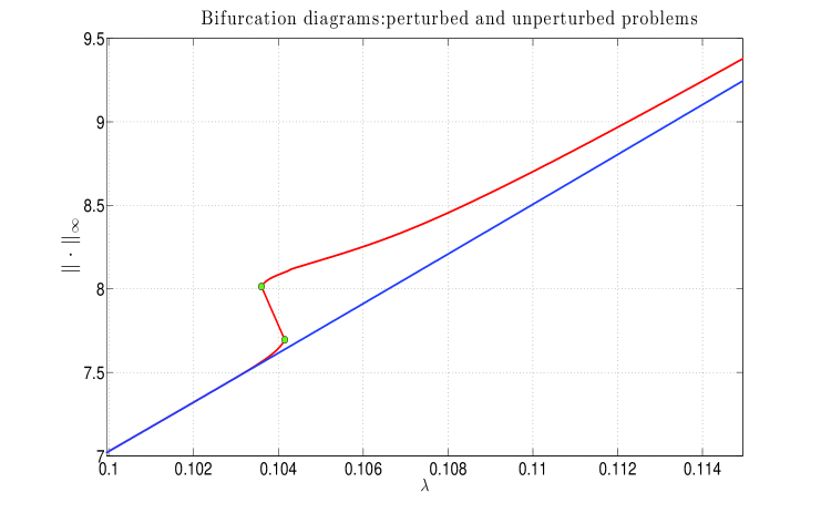
Figure 2. Bifurcation diagrams for the perturbed problem (red curve) and the unperturbed one (blue curve). The fold-points are indicated by the green dots.

The results are shown in Fig. 2. Compared to the set of stationary solutions associated with (4.1) (blue curve), the set of stationary solutions associated with (4.3) (red curve) exhibits two fold-points (green dots). Figure 2 represents actually a magnification of the discrepancies between these two solution sets. It has indeed been observed that the distance between the red and blue curves decays to zero (not shown) as $\lambda$ gets larger from its critical value $\lambda_{\mathfrak{c}}$ at which a discontinuity of the minimal branch occurs.

It is interesting to remark that $\lambda_{\mathfrak{c}}$ is here slightly bigger than $\lambda=0.104$ but smaller than $\lambda_{\mathfrak{s}}=0.11$, contrarily to Property (H₃) satisfied for a perturbation in $\mathcal{P}$ from Theorem 3.2. Here $\lambda_{\mathfrak{s}}$ corresponds to the parameter value from which the Gaussian perturbation $\varphi$ has been centered via $\|u_{\lambda_{\mathfrak{s}}}\|_{\infty}$, whereas for a perturbation in $\mathcal{P}$, $\|u_{\lambda_{\mathfrak{s}}}\|_{\infty}$ corresponds to a lower bound of the support of the perturbation.

It has been finally observed numerically that the emergence of fold-points such as reported on Fig. 2, persists when the perturbation $\varphi$ from (4.2) is still employed while $\varepsilon_{1}>0$ is further reduced. The rigorous justification of this observation boils down again essentially to an understanding of the mechanism at the origin of a discontinuity in the minimal branch, when this time a perturbation such as given in (4.2) is applied. We leave this issue for a future research, pointing out in the concluding remarks below a key element for the creation of such a discontinuity from the perturbation techniques of [CEP02].

5. Concluding remarks

The creation of a discontinuity in the minimal branch by arbitrarily small perturbations of the nonlinearity, has played a crucial role in the proof of Theorem 3.2. This is made possible when the spatial dimension is equal to one or two, due to the following observation regarding a specific Poisson equation used in the perturbation techniques of [CEP02].

Given $r>0$, one denote by $B_{r}$ the open ball of $\mathbb{R}^{d}$ of radius $r$, centered at the origin. For $0<\rho<R$, the solution $\Psi_{\rho}$ of the following Poisson equation

(5.1) $$\left\{\begin{array}[]{l}-\Delta\Psi_{\rho}=1_{B_{\rho}},\textrm{ in }B_{R},\\ \;\Psi_{\rho}|_{\partial B_{R}}=0,\end{array}\right.$$

satisfies for $\rho<R/2$,

(5.2) $$\underset{B_{2\rho}}{\inf}\Psi_{\rho}=\rho^{2}K(\rho),$$

where the behavior of $K(\rho)$ as $\rho\rightarrow 0$ is of the form

(5.3) $$K(\rho)\approx\left\{\begin{array}[]{l}R/\rho,\hskip 33.5001pt\textrm{ if }d=1,\\ |\log\rho|/2,\hskip 15.00002pt\textrm{ if }d=2.\end{array}\right.$$

This asymptotic behavior of $K(\rho)$ near $0$ can be proved by simply writing down the analytic expression of the solution to (5.1); see [CEP02, Lemma 3.1].

When $d\geq 3$, $K(\rho)$ converges to a constant (depending on $d$) as $\rho\rightarrow 0.$ This removal of the singularity at $0$ for $K$ in dimension $d\geq 3$, implies that the perturbation constructed from the techniques of [CEP02] needs to be sufficiently large to generate a discontinuity in the minimal branch. Whether this point is purely technical or more substantial, is still an open problem.

Appendix A Unbounded continuum of solutions to parametrized fixed point problems, in Banach spaces

We communicate in this appendix on a general result concerning the existence of an unbounded continuum of fixed points associated with one-parameter families of completely continuous perturbations of the identity map in a Banach space. This theorem is rooted in the seminal work of [LS34] that initiated what is known today as the Leray-Schauder continuation theorem. Extensions of such a continuation result can be found in [FMP86, MP84] for the multi-parameter case. Theorem A.1 below, formulates such a result in the one-parameter case. Its proof is provided here to make the expository as much self-contained as possible. Under a nonzero condition on the Leray-Schauder degree to hold at some parameter value, Theorem A.1 ensures in particular the existence of an unbounded continuum of solutions to nonlinear eigenvalue problems for which the nonlinearity is not necessarily Fréchet differentiable.

Results similar to Theorem A.1 that deal with the existence of an unbounded continuum of solutions to nonlinear eigenvalue problems, have been obtained in the literature, see e.g.  [Rab71, Theorem 3.2],  [Rab74, Corollary 1.34], [BB80, Theorem 3] or [Ama76, Theorem 17.1]. Similar to these works, the ingredients for proving Theorem A.1 rely also on the Leray-Schauder degree properties and connectivity arguments from point set topology. However, by following the approach of [FMP86, MP84], Theorem A.1 ensures the existence of an unbounded continuum of solutions to parameterized fixed point problems under more general conditions on the nonlinear term than required in [Rab71, Rab74, BB80, Ama76].

Hereafter, given a real Banach space $E$ and a map $\Psi:E\rightarrow E$, $\deg(\Psi,\mathcal{O},y)$ stands for the Leray-Schauder degree of $\Psi$ with respect to an open bounded subset $\mathcal{O}$ of $E$, and $y\in E.$ This degree is well defined for completely continuous perturbations $\Psi$ of the identity map and if $y\not\in\Psi(\partial\mathcal{O})$; see e.g.  [Dei85, Chap. 2,Thm. 8.1]. In what follows the $\lambda$-section of a nonempty subset $\mathcal{A}$ of $\mathbb{R}_{+}\times E$, is defined as:

(A.1) $$\mathcal{A}_{\lambda}:=\{u\in E\;:\;(\lambda,u)\in\mathcal{A}\}.$$

Theorem A.1.

Let $\mathcal{U}$ be an open bounded subset of a real Banach space $E$ and assume that $G:\mathbb{R}_{+}\times E\rightarrow E$ is completely continuous (i.e.  compact and continuous). We assume that there exists $\lambda_{0}\geq 0$, such that the equation,

(A.2) $$u-G(\lambda_{0},u)=0$$

has a unique solution $u_{0}$, and,

(A.3) $$\deg(I-G(\lambda_{0},\cdot),\mathcal{U},0)\neq 0.$$

Let us introduce

(A.4) $$\mathcal{S}^{+}=\{(\lambda,u)\in[\lambda_{0},\infty)\times E:u=G(\lambda,u)\}.$$

Then there exists a continuum $\mathcal{C}^{+}\subseteq\mathcal{S}^{+}$ (i.e. a closed and connected subset of $\mathcal{S}^{+}$) such that the following properties hold:

• $\mathcal{C}_{\lambda_{0}}^{+}\cap\mathcal{U}=\{u_{0}\}$,

• Either $\mathcal{C}^{+}$ is unbounded or $\mathcal{C}_{\lambda_{0}}^{+}\cap(E\setminus\overline{\mathcal{U}}))\neq\emptyset.$

To prove this theorem, we need an extension of the standard homotopy property of the Leray-Schauder degree [Dei85, p. 56] to homotopy cylinders that exhibit variable $\lambda$-sections. This is the purpose of the following Lemma.

Lemma A.1.

Let $\mathcal{O}$ be a bounded open subset of $[\lambda_{1},\lambda_{2}]\times E$, and let $G:\overline{\mathcal{O}}\rightarrow E$ be a completely continuous mapping. Assume that $u\neq G(\lambda,u)$ on $\partial\mathcal{O},$ then for all $\lambda\in[\lambda_{1},\lambda_{2}]$,

$$\deg(I-G(\lambda,\cdot),\mathcal{O}_{\lambda},0_{E})\mbox{ is independent of }\lambda,$$

where $\mathcal{O}_{\lambda}=\{u\in E\;:\;(\lambda,u)\in\mathcal{O}\}$ is the $\lambda$-section of $\mathcal{O}$.

Proof.

We may assume, without loss of generality, that $\mathcal{O}\neq\emptyset$ and that $\lambda_{1}=\inf\{\lambda:\mathcal{O}_{\lambda}\neq\emptyset\}$ and $\lambda_{2}=\sup\{\lambda:\mathcal{O}_{\lambda}\neq\emptyset\}.$ Consider $\varepsilon>0$ and the following superset of $\mathcal{O}$ in $\mathbb{R}\times E,$

(A.5) $$\mathcal{O}^{\varepsilon}:=\mathcal{O}\bigcup\Big{(}(\lambda_{1}-\varepsilon,\lambda_{1})\times\mathcal{O}_{\lambda_{1}}\cup(\lambda_{2},\lambda_{2}+\varepsilon)\times\mathcal{O}_{\lambda_{2}}\Big{)}.$$

Then $\mathcal{O}^{\varepsilon}$ is an open bounded subset of $\mathbb{R}\times E.$ Since $\overline{\mathcal{O}}$ is closed by definition and $G$ is continuous, then according to the Dugundgi extension theorem on metric spaces [Dug66, Thm. 6.1 p. 188] (cf. Lemma B.2 below), $G$ can be extended to $\mathbb{R}\times E$ as a continuous function that we denote by $\widetilde{G}$.

Now consider,

$$\forall\;(\lambda,u)\in\mathbb{R}\times E,\;H(\lambda,u):=(\lambda-\lambda^{\ast};u-\widetilde{G}(\lambda,u)),$$

with some arbitrary fixed $\lambda^{\ast}\in[\lambda_{1},\lambda_{2}]$. Then $H$ is a completely continuous perturbation of the identity in $\mathbb{R}\times E$. In what follows, one denotes by $\widetilde{E}$ the set $\mathbb{R}\times E$.

Since $H(\lambda,u)=0_{\widetilde{E}}$ if and only if $\lambda=\lambda^{\ast}$ and $u=\widetilde{G}(\lambda,u),$ and since $\lambda^{\ast}\in[\lambda_{1},\lambda_{2}]$ and $G(\lambda,u)\neq u$ on $\partial\mathcal{O}$ by assumptions, we deduce that,

(A.6) $$\forall\;(\lambda,u)\in\partial\mathcal{O}^{\varepsilon},\;H(\lambda,u)\neq 0_{\widetilde{E}}.$$

Therefore $\deg(H,\mathcal{O}^{\varepsilon},0_{\widetilde{E}})$ is well defined and constant.

Let us consider the following one-parameter family $\{H_{t}\}_{t\in[0,1]}$ of perturbations of $H$ defined by,

$$\forall\;(\lambda,u)\in\mathbb{R}\times E,\;H_{t}(\lambda,u):=(\lambda-\lambda^{\ast};u-t\widetilde{G}(\lambda,u)-(1-t)\widetilde{G}(\lambda^{*},u)).$$

Then

(A.7) $$\Big{(}H_{t}(\lambda,u)=0\Big{)}\Leftrightarrow\Big{(}\lambda=\lambda^{\ast}\mbox{ and }u=\widetilde{G}(\lambda^{*},u)\Big{)},$$

and from our assumptions, we conclude again that $H_{t}(\lambda,u)\neq 0_{\widetilde{E}}$ for all $(\lambda,u)\in\partial\mathcal{O}^{\varepsilon}$ and all $t\in[0,1]$.

By applying now the standard homotopy invariance principle to the family $\{H_{t}\}_{t\in[0,1]}$ we have

(A.8) $$\deg(H_{1},\mathcal{O}^{\varepsilon},0_{\widetilde{E}})=\deg(H,\mathcal{O}^{\varepsilon},0_{\widetilde{E}})=\deg(H_{0},\mathcal{O}^{\varepsilon},0_{\widetilde{E}}).$$

Let $K$ be the closed subset of $\overline{\mathcal{O}^{\varepsilon}}$ such that $\mathcal{O}^{\varepsilon}\backslash K=(\lambda_{1}-\varepsilon,\lambda_{2}+\varepsilon)\times\mathcal{O}_{\lambda^{\ast}}.$ Then $0_{\widetilde{E}}$ does not belong to $H(\partial\mathcal{O}^{\varepsilon}\cup K)$ since the cancelation of $H$ is possible only on the $\lambda^{\ast}$-cross section, while $K$ does not intercept this section by construction and $0_{\widetilde{E}}\not\in H(\partial\mathcal{O}^{\varepsilon})$ from (A.6). By applying now the excision property of the Leray-Schauder degree [Dei85, Nir01] with such a $K$, we obtain,

(A.9) $$\deg(H_{0},\mathcal{O}^{\varepsilon},0_{\widetilde{E}})=\deg(H_{0},(\lambda_{1}-\varepsilon,\lambda_{2}+\varepsilon)\times\mathcal{O}_{\lambda^{\ast}},0_{\widetilde{E}}).$$

The interest of (A.9) relies on the fact that the degree is by this way expressed on a cartesian product which allows us to apply the cartesian product formula (see Lemma B.1) and gives in our case

(A.10) $$\deg(H_{0},(\lambda_{1}-\varepsilon,\lambda_{2}+\varepsilon)\times\mathcal{O}_{\lambda^{\ast}},0_{\widetilde{E}})=\deg(I-G(\lambda^{\ast},\cdot),\mathcal{O}_{\lambda^{\ast}},0_{E}),$$

since $\deg(f,(\lambda_{1}-\varepsilon,\lambda_{2}+\varepsilon),0_{\mathbb{R}})=1$ with $f(\lambda)=\lambda-\lambda^{*},$ and $\lambda^{*}\in[\lambda_{1},\lambda_{2}]$.

By applying now (A.10), (A.9) and (A.8) and by recalling that $\deg(H,\mathcal{O}^{\varepsilon},0_{\widetilde{E}})$ is independent of $\lambda^{*}$, we have thus proved that for arbitrary $\lambda^{*}\in[\lambda_{1},\lambda_{2}],$ $\deg(I-G(\lambda^{\ast},\cdot),\mathcal{O}_{\lambda^{\ast}},0_{E})$ is also independent of $\lambda^{*}.$ The proof is complete. ∎

Remark A.1.

The introduction of $\mathcal{O}^{\varepsilon}$ such as defined in (A.5) above was used in order to work within an open bounded subset of a Banach space, here $\mathbb{R}\times E$, and thus to work within the framework of the Leray-Schauder degree. The Dugundgi theorem is used to appropriately extend the mapping $G$ to $\mathcal{O}^{\varepsilon}$ in order to apply the Leray-Schauder degree techniques.

The last ingredient to prove Theorem A.1, is the following separation lemma from point set topology (Lemma A.2 below). A separation of a topological space $X$ is a pair of nonempty open subsets $U$ and $V$, such that $U\cap V=\emptyset$ and $U\cup V=X$. A space is connected if it does not admit a separation. Two subsets $A$ and $B$ are connected in $X$ if the exists a connected set $Y\subset X,$ such that $A\cap Y\neq\emptyset$ and $B\cap Y\neq\emptyset$. Two nonempty subsets $A$ and $B$ of $X$ are separated if there exists a separation $U,V$ of $X$ such that $A\subseteq U$ and $B\subseteq V.$ There exists a relationship between these concepts in the case where $X$ compact, this is summarized in the following separation lemma.

Lemma A.2.

(Separation lemma) If $X$ is compact and $A$ and $B$ are not separated, then $A$ and $B$ are connected in $X$.

The proof of this lemma may be found in [Dei85, Lemma 29.1]; see also [Kur68].

As a result if two subsets of a compact set are not connected, they are separated. We are now in position to prove Theorem A.1.

Proof of Theorem A.1.

Proof.

Let $\mathcal{C}^{+}$ be the maximal connected subset of $\mathcal{S}^{+}$ such that (i) holds, which is trivial by assumptions. We proceed by contradiction. Assume that $\mathcal{C}^{+}_{\lambda_{0}}\cap(E\setminus\overline{\mathcal{U}})=\emptyset$ and that $\mathcal{C}^{+}$ is bounded in $[\lambda_{0},\infty)\times E$. Then there exists a constant $R>0$ such that for each $(\lambda,u)\in\mathcal{C}^{+}$ we have $\|u\|+|\lambda|<R$. Introduce,

$$\mathcal{S}^{+}_{2R}:=\{(\lambda,u)\in\mathcal{S}^{+}\;:\;\|u\|+|\lambda|\leq 2R\}.$$

From the complete continuity of $G$ it follows that any set of the form $\mathcal{H}:=\{(\lambda,u)\in\Lambda\times E\;:\;u=G(\lambda,u)\},$ with $\Lambda$ a closed and bounded subset of $[\lambda_{0},\infty),$ is a compact subset of $[\lambda_{0},\infty)\times E$. As a result, $\mathcal{S}^{+}_{2R}$ is a compact subset of $[\lambda_{0},\infty)\times E$.

There are two possibilities. Either (a) $\mathcal{S}^{+}_{2R}=\mathcal{C}^{+}$ or, (b) there exists $(\lambda^{*},u^{*})\in\mathcal{S}^{+}_{2R}$ such that $(\lambda^{*},u^{*})$ does not belong to $\mathcal{C}^{+}$.

Let $\mathcal{U}$ be as defined in Theorem A.1. Consider case (b) first. We want to apply Lemma A.2 with $X=\mathcal{S}^{+}_{2R},$ $A=\mathcal{C}^{+},$ and $B=\{\lambda^{*}\}\times\mathcal{S}_{2R}^{+}$. Obviously, $A$ and $B$ are not connected in $\mathcal{S}^{+}_{2R}$ since $(\lambda^{*},u^{*})\not\in\mathcal{C}^{+}$ and $\mathcal{C}^{+}$ is the maximal connected subset of $\mathcal{S}^{+}$. We may therefore apply Lemma A.2 in such a case and build an open subset $\mathcal{O}$ of $[\lambda_{0},\infty)\times E$, such that the following properties hold,

• $\mathcal{O}_{\lambda_{0}}=\mathcal{U}$ (since $\mathcal{C}^{+}_{\lambda_{0}}\cap(E\setminus\overline{\mathcal{U}})=\emptyset$),

• $\mathcal{C}^{+}\subset\mathcal{O}$,

• $\mathcal{S}^{+}_{2R}\cap\partial\mathcal{O}=\emptyset$ and,

• $\mathcal{O}_{\lambda^{*}}$ contains no solutions of $u=G(\lambda^{*},u)$.

The last property comes from the fact that $A$ and $B$, as defined above, are separated.

From (c₃), we get by applying Lemma A.1, that,

(A.11) $$\forall\;\lambda\in\Lambda_{R},\;\deg(I-G(\lambda,\cdot),\mathcal{O}_{\lambda},0)=\deg(I-G(\lambda_{0},\cdot),\mathcal{O}_{\lambda_{0}},0),$$

where $\Lambda_{R}$ denotes the projection of $\mathcal{S}^{+}_{2R}$ onto $[\lambda_{0},\infty)$.

Now $\deg(I-G(\lambda_{0},\cdot),\mathcal{O}_{\lambda_{0}},0)\neq 0$ by (c₁) and the assumptions of Theorem A.1. We obtain therefore a contradiction from (c₄) when (A.11) is applied for $\lambda=\lambda^{*}$ .

The case $\mathcal{C}^{+}=\mathcal{S}^{+}_{2R},$ may be treated along the same lines and is left to the reader. The proof is complete. ∎

Remark A.2.

Theorem A.1 shows in particular that if for all $\mathcal{U}$ there is a unique solution $(\lambda_{0},u_{0})$ in $\mathcal{U}$, of $u=G(\lambda_{0},u)$, then there exists an unbounded continuum of solutions of $u=G(\lambda,u),$ provided that there exists an open set $\mathcal{V}$ in $E$ such that $\deg(I-G(\lambda_{0},\cdot),\mathcal{V},0)\neq 0$.

Remark A.3.

It is not essential that $u_{0}$ be the only solution of (A.2) in $\mathcal{U}$. If one only assumes (A.3), one obtains the existence of finitely many continua satisfying the alternative formulated in (ii) of Theorem A.1.

Appendix B Product formula for the Leray-Schauder degree, and the Dugundji extension theorem

This appendix contains auxiliaries lemmas used in the previous Appendix. We first start with the cartesian product formula for the Leray-Schauder degree.

Lemma B.1.

Assume that $\mathcal{U}=\mathcal{U}_{1}\times\mathcal{U}_{2}$ is a bounded open subset of $E_{1}\times E_{2}$, where $E_{1}$ and $E_{2}$ are two real Banach spaces with $\mathcal{U}_{1}$ and $\mathcal{U}_{2}$ open subsets of $E_{1}$ and $E_{2}$ respectively. Suppose that for all $x=(x_{1},x_{2})\in E$, $f(x)=(f_{1}(x_{1}),f_{2}(x_{2})),$ where $f_{1}:\overline{\mathcal{U}_{1}}\rightarrow E_{1}$ and $f_{2}:\overline{\mathcal{U}_{2}}\rightarrow E_{2}$ are continuous and suppose that $y=(y_{1},y_{2})\in E$ is such that $y_{1}$ (resp. $y_{2}$) does not belong to $f_{1}(\partial\mathcal{U}_{1})$ (resp. $f_{2}(\partial\mathcal{U}_{2})$). Then,

$$\deg(f,\mathcal{U},y)=\deg(f_{1},\mathcal{U}_{1},y_{1})\deg(f_{2},\mathcal{U}_{2},y_{2}).$$

We recall below the Dugundgi extension theorem [Dug66, Thm. 6.1 p. 188].

Lemma B.2.

(Dugundgi) Let $E$ and $X$ be Banach spaces and let $f:\mathfrak{C}\rightarrow E$ a continuous mapping, where $\mathfrak{C}$ is a closed subset of $E$. Then there exists a continuous mapping $\widetilde{f}:E\rightarrow K$ such that $\widetilde{f}(u)=f(u)$ for all $u\in\mathfrak{C}$.

Proof.

(Sketch) For each $u\in E\backslash\mathfrak{C},$ let $r_{u}=\frac{1}{3}\mbox{dist}(u,\mathfrak{C}),$ and $B_{u}:=\{v\in E\;:\;\|v-u\|<r_{u}\}$. Then $\mbox{diam}(B_{u})\leq\mbox{dist}(B_{u},\mathfrak{C}),$ and $\{B_{u}\}_{u\in E\backslash\mathfrak{C}}$ is a open cover of $E\backslash\mathfrak{C}$ which admits a local refinement $\{\mathcal{O}_{\lambda}\}_{\lambda\in\Lambda}$: i.e. $\underset{\lambda\in\Lambda}{\bigcup}\mathcal{O}_{\lambda}\supset E\backslash\mathfrak{C}$, for each $\lambda\in\Lambda$ there exists $B_{u}$ such that $B_{u}\supset\mathcal{O}_{\lambda}$, and every $u\in E\backslash\mathfrak{C}$ has a neighborhood $U$ such that  $U$ intersects at most finitely many elements of $\{\mathcal{O}_{\lambda}\}_{\lambda\in\Lambda}$ (locally finite family).

Introduce now $\gamma:E\backslash\mathfrak{C}\rightarrow\mathbb{R}^{+}_{*}$, defined by $\gamma(u)=\underset{\lambda\in\Lambda}{\sum}\mbox{dist}(u,\overline{\mathcal{O}_{\lambda}})$ and introduce

$$\forall\lambda\in\Lambda,\;\forall u\in E\backslash\mathfrak{C},\;\;\gamma_{\lambda}(u)=\frac{\mbox{dist}(u,\overline{\mathcal{O}_{\lambda}})}{\gamma(u)}.$$

By construction, the above sum over $\Lambda$ contains only finitely many terms and thus $\gamma$ is continuous.

Now define $\widetilde{f}$ by,

(B.1) $$\widetilde{f}=\left\{\begin{array}[]{l}f(u),\mbox{ if }u\in\mathfrak{C},\\ \sum_{\lambda\in\Lambda}\gamma_{\lambda}(u)f(u_{\lambda}),\;u\not\in\mathfrak{C}.\end{array}\right.$$

Then it can be shown that $\widetilde{f}$ is continuous.

∎

References

- [AM87] R. Abraham and J.E. Marsden, Foundations of mechanics, Addison-Wesley Publishing Company, Inc., 1987.
- [Ama76] H. Amann, Fixed point equations and nonlinear eigenvalue problems in ordered Banach spaces, SIAM Review, 18 (1976), 620-709.
- [AP37] A.A. Andronov, and L.S. Pontryagin, Systèmes grossiers, Dokl. Akad. Nauk. SSSR, 14 (5), 1937, 247-250.
- [Arn81] V. I. Arnol’d, Singularity theory, vol. 53, Cambridge University Press, 1981.
- [Arn83] V. I. Arnol’d, Geometrical Methods in the Theory of Ordinary Differential Equations, Grundlehren der Mathematischen Wissenschaften, vol. 250, Springer-Verlag, New York, 1983, Translated from the Russian by Joseph Szücs, Translation edited by Mark Levi.
- [BE89] J. Bebernes, and D. Eberly, Mathematical Problems From Combustion Theory, Springer-Verlag, 1989.
- [Ben10] N. Ben-Gal, Grow-Up Solutions and Heteroclinics to Infinity for Scalar Parabolic PDEs, Ph.D. Thesis, Division of Applied Mathematics, Brown University, 2010.
- [BCT88a] M. Berger, P. Church, and J. Timourian, Folds and cusps in Banach spaces, with applications to nonlinear partial differential equations. I, Indiana Univ. Math. J. 34 (1985) (1), 1 19.
- [BCT88b] by same author, Folds and cusps in Banach spaces, with applications to nonlinear partial differential equations. II, Trans. Amer. Math. Soc. 307 (1988), 225–244.
- [BB80] H. Brezis and H. Berestycki, On a free boundary problem arising in plasma physics, Nonlinear Analysis 4 (1980), 415–436.
- [BO86] H. Brezis and L. Oswald, Remarks on sublinear elliptic equations, Nonlinear Analysis: Theory, Methods and Applications, 10 (1), 55–64, 1986.
- [BCMR96] H. Brezis, T. Cazenave, Y. Martel, and A. Ramiandrisoa, Blow up for revisited, Adv. Differential Equations 1 (1996), 73-90.
- [BV97] H. Brezis, and J. L. Vázquez, Blow-up solutions of some nonlinear elliptic problems. Rev. Mat. Univ. Compl. Madrid, 10, 1997, 443-469.
- [BF82] F. Brezzi and H. Fujii, Numerical imperfections and perturbations in the approximation of nonlinear problems, 1982.
- [BRR80] F. Brezzi, J. Rappaz, and P.A. Raviart, Finite dimensional approximation of nonlinear problems, Numerische Mathematik 36 (1980), no. 1, 1–25.
- [BIS81] K. J. Brown, M. M. A. Ibrahim, and R. Shivaji, S-shaped bifurcation curves, Nonlinear Anal.: Theory, Methods, and Applications, 5 (1981), 475–486.
- [BP97] P. Brunovský and P. Poláik, The Morse-Smale structure of a generic reaction-diffusion equation in higher space dimension, Journal of Differential Equation, 135 (1997), 129–181.
- [CS84] A. Castro and R. Shivaji, Uniqueness of positive solutions for a class of elliptic boundary value problems, Proc. Royal Soc. Edinburgh Sect. A 98 (1984), 267–269.
- [Caz06] T. Cazenave, An Introduction to Semilinear Elliptic Equations, Editora do Instituto de Matemática, Universidade Federal do Rio de Janeiro, 2006.
- [CEP02] T. Cazenave, M. Escobedo, and A. Pozio. Some stability properties for minimal solutions of , Portugaliae Mathematica, 59 (2002), 373–391.
- [CH98] T. Cazenave and A. Haraux, An Introduction to Semilinear Evolution Equations, Oxford Lecture Series in Mathematics and its Applications, vol. 13, The Clarendon Press Oxford University Press, New York, 1998, Translated from the 1990 French original by Yvan Martel and revised by the authors.
- [Cha57] S. C. Chandrasekhar, An Introduction to the Study of Stellar Structure, Dover Publ., N. Y., 1957.
- [CGVR06] M. D. Chekroun, M. Ghil, J. Roux and F. Varadi, Averaging of time-periodic systems without a small parameter, Disc. and Cont. Dyn. Syst. A, 14 (2006), 753–782.
- [CR13] M. D. Chekroun, and J. Roux, Homeomorphism groups of normed vector space: The conjugacy problem and the Koopman operator, Disc. and Cont. Dyn. Syst. A, 33 (9) (2013), 3957–3980.
- [CPT16] M. D. Chekroun, E. Park, and R.Temam, The Stampacchia maximum principle for stochastic partial differential equations and applications, Journal of Differential Equations, 260 (3) (2016), 2926–2972.
- [CKL17] M. D. Chekroun, A. Kroener, and H. Liu, Galerkin approximations of nonlinear optimal control problems in Hilbert spaces, Electron. J. Differential Equations, 2017 (189) (2017), 1–40.
- [CHMP75] S.-N. Chow, J. K. Hale and J. Mallet-Paret, Applications of generic bifurcation, I, Arch. Rat. Mech. Anal. 59 (1975), 159–188.
- [CH82] S.-N. Chow, and J. K. Hale, Methods of Bifurcation Theory, Grundlehren der Mathematischen Wissenschaften, vol. 251, Springer-Verlag, New York/Berlin, 1982.
- [CT97] P. T. Church and J. G. Timourian, Global structure for nonlinear operators in differential and integral equations. I. Folds; II. Cusps: Topological nonlinear analysis, in “Progr. Nonlinear Differential Equations Appl.,” 27, pp. 109–160, 161–245, Birkhauser, Boston, 1997.
- [CR73] M. G. Crandall, and P.H. Rabinowitz, Bifurcation, perturbation of simple eigenvalues and linearized stability, Arch. Rational Mech. Anal., 52 (1973), 161-180.
- [CR75] M. G. Crandall, and P. H. Rabinowitz, Some continuation and variational methods for positive solutions of nonlinear elliptic eigenvalue problems, Arch. Rational Mech. Anal. 58 (1975), 207–218.
- [DPF90] N. Damil, and M. Potier-Ferry, A new method to compute perturbed bifurcations: application to the buckling of imperfect elastic structures, International Journal of Engineering Science 28 (1990), no. 9, 943–957.
- [Dan88] E. N. Dancer, The effect of domain shape on the number of positive solutions of certain nonlinear equations, J. Diff. Eqns, 74 (1988), 120–156.
- [Dan08] E. N. Dancer, Domain perturbation for linear and semi-linear boundary value problems, Handbook of Differential Equations: Stationary Partial Differential Equations, Vol 6, (M. Chipot, Editor), Elsevier, 2008.
- [Dei85] K. Deimling, Nonlinear Functional Analysis, Springer, Berlin, 1985.
- [Du00] Y. Du, Exact multiplicity and S-shaped bifurcation curve for some semilinear elliptic problems from combustion theory, SIAM J. Math. Analysis, 32 (2000), 707–733.
- [DL01] Y. Du, and Y. Lou, Proof of a conjecture for the perturbed Gelfand equation from combustion theory, J. Differential Equations, 173 (2001), 213–230.
- [Dug66] J. Dugundji, Topology, Allyn and Bacon, Boston, 1966.
- [FR99] B. Fiedler, and C. Rocha, Orbit equivalence of global attractors of semilinear parabolic differential equations, Transactions of the American Mathematical Society, 352 (1) (1999), 257–284.
- [FP99] M. Fila, and P. Poláčik, Global solutions of a semilinear parabolic equation, Advances in Differential Equations 4 (2) (1999), 163–196.
- [Fil05] M. Fila, Blow-up of solutions of supercritical parabolic equations, 105-158, in Handbook of Differential Equations: Evolutionary Equations, Vol. 2, Amsterdam: Elsevier, 2005.
- [FMP86] P. M. Fitzpatrick, I. Massabo and J. Pejsachowicz, On the covering dimension of the set of solutions of some nonlinear equations, Trans. Amer. Math. Soc. 296 (1986), 777-798.
- [F-K69] D. A. Frank-Kamenetskii, Diffusion and Heat Transfert in Chemical Kinematics, –edition, Plenum Press, 1969.
- [Fuj69] H. Fujita, On the nonlinear equations and , Bull. Amer. Math. Soc. 75 (1969), 132-135.
- [Gel63] I.M. Gel’fand, Some problems in the theory of quasilinear equations, Amer. Math. Soc. Transl. 29 (1963), 295-381.
- [GT98] D. Gilbarg and N.S. Trudinger, Elliptic Partial Differential Equations of Second Order, Springer, reprint of the 2nd ed. Berlin-Heidelberg-New York (1983), Corr. 3rd printing, 1998.
- [GS79] M. Golubitsky and D Schaeffer, A theory for imperfect bifurcation via singularity theory, Communications on Pure and Applied Mathematics 32 (1979), no. 1, 21–98.
- [GS85] by same author, Singularities and Groups in Bifurcation Theory, Vol. I, Applied Mathematical Sciences vol. 51, Springer, 1985.
- [Hal88] J.K. Hale, Asymptotic Behaviour of Dissipative systems, Amer. Math. Soc., Providence, RI, 1988.
- [HMO02] J.K. Hale, L.T. Magalhães and W.M. Oliva, Dynamics in Infinite Dimensions, 2nd Ed. Springer-Verlag, 2002.
- [HI11] M. Haragus and G. Iooss, Local Bifurcations, Center Manifolds, and Normal Forms in Infinite-Dimensional Dynamical Systems, Universitext, Springer-Verlag, London, 2011.
- [Hen81] D. Henry, Geometric Theory of Semilinear Parabolic Equations, Lecture Notes in Mathematics, vol. 840, Springer-Verlag, Berlin, 1981.
- [Hen05] D. Henry, Perturbation of the Boundary in Boundary-value Problems of Partial Differential Equations, London Mathematical Society Lecture Note Series, vol. 318, Cambridge University Press, Cambridge, 2005.
- [Hir76] M.W. Hirsch, Differential Topology, Graduate Texts in Mathematics, 33, Springer–Verlag, 1976.
- [JL73] D.D. Joseph, T.S. Lundgren, Quasilinear Dirichlet problems driven by positive sources, Arch. Rational Mech. Anal. 49 (1973), 241–269.
- [KH97] A. Katok and B. Hasselblatt, Introduction to the Modern Theory of Dynamical Systems, With a supplement by Anatole Katok and Leonardo Mendoza, Encyclopedia of Mathematics and Its Applications 54, Cambridge University Press, 1997.
- [KK73] J.P. Keener and H.B. Keller, Perturbed bifurcation theory, Archive for rational mechanics and analysis 50 (1973), no. 3, 159–175.
- [Kie12] H. Kielhöfer, Bifurcation Theory: An Introduction with Applications to Partial Differential Equations, 156, Springer, 2012.
- [KL99] Korman, P. and Li, Y. On the exactness of an S-shaped bifurcation curve, Proc. Amer. Math. Soc., 127 (1999) 1011 1020.
- [Kur68] K. Kuratowski, Topology, vol. 2, Academic Press, New York, 1968.
- [Kuz04] Yu.A. Kuznetsov, Elements of Applied Bifurcation Theory, Springer, 3rd edition, 2004.
- [LS34] J. Leray, and J. Schauder, Topologie et équations fonctionnelles, Ann. Sci. École Norm. Sup. 51 (3) (1934), 45–78; Russian transl. in Uspekhi Mat. Nauk 1 (1946), No. 3 4, 71-95.
- [Lio82] P.L. Lions, On the existence of positive solutions of semilinear elliptic equations, SIAM. Rev, 24 (1982), 441–467.
- [Lu94] K. Lu, Structural stability for scalar parabolic equations, Journal of Differential Equations, 114 (1994), 253–271.
- [LLMP05] L. Lorenzi, A. Lunardi, G. Metafune, and D. Pallara, Analytic Semigroups and Reaction-Diffusion Problems, 8th International Internet Seminar on Evolution Equations, (2005).
- [Lun95] A. Lunardi, Analytic Semigroups and Optimal Regularity in Parabolic Problems, Birkhäuser, Basel, 1995.
- [MWZ02] Q. Ma, S. Wang, and C. Zhong, Necessary and sufficient conditions for the existence of global attractors for semigroups and applications, Indiana Univ. Math. J., 51 (6) (2002), 1541–1559.
- [MW05] T. Ma and S. Wang, Bifurcation Theory and Applications, World Scientific Series on Nonlinear Science. Series A: Monographs and Treatises, vol. 53, World Scientific Publishing Co. Pte. Ltd., Hackensack, NJ, 2005.
- [MW14] by same author, Phase Transition Dynamics, Springer-Verlag, 2014.
- [MP84] I. Massabo and J. Pejsachowicz, On the connectivity properties of the solution set of parametrized families of compact vector fields, J. Funct. Anal. 59 (1984), 151 166.
- [MM76] J.E. Marsden and M. McCracken, The Hopf Bifurcation and Its Applications, vol. 19, Springer-Verlag, 1976.
- [Mat82] H. Matano, Nonincrease of the lap-number of a solution for a one-dimensional semilinear parabolic equation, Journal of the Faculty of Science: University of Tokyo: Section IA, 29, 401–441, 1982.
- [Min04] T. Minamoto, Numerical method with guaranteed accuracy of a double turning point for a radially symmetric solution of the perturbed Gelfand equation, J. of Comput. and App. Math., 169 (2004) 151–160.
- [MN07] T. Minamoto and M.T. Nakao, Numerical method for verifying the existence and local uniqueness of a double turning point for a radially symmetric solution of the perturbed gelfand equation, Journal of computational and applied mathematics 202 (2007), no. 2, 177–185.
- [MS80] G. Moore and A. Spence, The calculation of turning points of nonlinear equations, SIAM Journal on Numerical Analysis 17 (1980), no. 4, 567–576.
- [NS94] K. Nagasaki, and T. Suzuki, Spectral and related properties about the Emden-Fowler equation on circular domains, Math. Ann. 299 (1994), 1–15.
- [New11] S. E. Newhouse, Lectures on Dynamical Systems, Springer, 2011.
- [Nir01] L. Nirenberg, Topics in Nonlinear Functional Analysis, Courant Lecture Notes, AMS/CLN 6, 2001.
- [OS99] T. Ouyang, and J. Shi, Exact multiplicity of positive solutions for a class of semilinear problem, II, J. Differential Equations 158 (1999), 94-151.
- [Paz83] A. Pazy, Semigroups of Linear Operators and Applications to Partial Differential Equations, Springer-Verlag, New York, 1983.
- [QS07] P. Quittner, and P. Souplet, Superlinear Parabolic Problems: Blow-up, Global existence and Steady states, Springer, 2007.
- [Rab71] P. H. Rabinowitz, Some global results for nonlinear eigenvalue problems, J. Funct. Anal., 7, (1971), 487–513.
- [Rab73] P. H. Rabinowitz, Some aspects of nonlinear eigenvalue problems, Rocky Mountain J. Math., 3 (2) (1973), 161-202.
- [Rab74] P. H. Rabinowitz, Pairs of positive solutions of nonlinear elliptic partial differential equations, Indiana Univ. Math. J. 23 (1974), 173–186.
- [Rob01] J. Robinson, Infinite-Dimensional Dynamical Dystems, Cambridge Texts in Applied Mathematics, Cambridge University Press, Cambridge, 2001.
- [RCCS14] L. Roques, M.D. Chekroun, M. Cristofol, S. Soubeyrand, and M. Ghil, Parameter estimation for energy balance models with memory, Proc. Roy. Soc. A 470 (2014), 20140349. (doi:10.1098/rspa.2014.0349)
- [RC07] L. Roques, and M.D. Chekroun, On population resilience to external perturbations, SIAM Journal on Applied Mathematics, 68 (1) (2007), 133–153.
- [Sat73] D. H. Sattinger, Topics in Stability and Bifurcation Theory, Springer, 1973.
- [Sat80] D. H. Sattinger, Bifurcation and symmetry breaking in applied mathematics, Bulletin of the American Mathematical Society 3 (1980), no. 2, 779–819.
- [SY02] G. Sell, and Y. You, Dynamics of Evolutionary Equations, Springer-Verlag, New York, 2002.
- [She80] M. Shearer, One-parameter perturbations of bifurcation from a simple eigenvalue, Math. Proc. Cambridge Philos. Soc. 88 (1980) (1), 111 123.
- [SW82] A. Spence, and B. Werner, Non-simple turning points and cusps, IMA Journal of Numerical analysis, 2 (1982), no. 4, 413–427.
- [Sma67] S. Smale, Differentiable dynamical systems, Bull. Amer. Math. Soc., 73 (1967), 747–817.
- [Tai95] K. Taira, Analytic Semigroups and Semilinear Initial Boundary Value Problems, London Mathematical Society Lecture Note Series, Cambridge University Press, 223, 1995.
- [Tai98] K. Taira, Bifurcation theory for semilinear elliptic boundary value problems, Hiroshima Math. J., 28 (1998), 261–308.
- [Tem75] R. Temam, A nonlinear eigenvalue problem: the shape of equilibrium of a confined plasma, Arch. Rational Mech. Anal. 60, 51–73 (1975).
- [Tem97] R. Temam, Infinite-Dimensional Dynamical Systems in Mechanics and Physics, 2nd ed., Applied Mathematical Sciences, vol. 68, Springer-Verlag, New York, 1997.
- [ZWS07] Y. Zhao, Y. Wang and J. Shi, Exact multiplicity of solutions and S-shaped bifurcation curve for a class of semi-linear elliptic equations from a chemical reaction model, J. Math. Anal. Appl., 331 (2007), 263–278.