ABSTRACT

Radiative emission of neutrino pair (RENP) from atomic states is a new tool to experimentally investigate undetermined neutrino parameters such as the smallest neutrino mass, the nature of neutrino masses (Majorana vs Dirac), and their CP properties. We study effects of neutrino pair emission either from nucleus or from inner core electrons in which the zero-th component of quark or electron vector current gives rise to large coupling. Both the overall rate and the spectral shape of photon energy are given for a few cases of interesting target atoms. Calculated rates exceed those of previously considered target atoms by many orders of magnitudes.

Key words

Neutrino mass, Majorana particles, Macro-coherence

I Introduction

Recent developments of neutrino oscillation experiments have achieved remarkable success: many elements of the fundamental neutrino mass matrix have been determined, including all three mixing angles and two mass squared differences [1]. They however left undetermined the absolute scale of neutrino masses (or equivalently the smallest neutrino mass), the nature of masses (Dirac or Majorana type), and their CP properties. Conventional targets in ongoing experiments of exploring these undetermined neutrino properties and parameters have been nuclei. Direct measurement of the end point spectrum of beta decay such as tritium [2] and (neutrino-less) double beta decay [3] are two main methods to resolve these outstanding problems.

Some time ago we proposed to use atomic transitions for improved exploration of undetermined neutrino properties [4], [5]. The idea is to exploit the fact that atomic level spacings are much closer to expected neutrino masses and many experimental methods are available to manipulate atomic transitions. The process we use is atomic de-excitation; $|e\rangle\rightarrow|g\rangle+\gamma+\nu_{i}\nu_{j}$ where $\nu_{i},i=1,2,3$ are neutrino mass eigen states. By measuring the photon energy spectral shape and determining locations of six thresholds at $\omega_{ij}\equiv\epsilon_{eg}/2-(m_{i}+m_{j})^{2}/(2\epsilon_{eg})$ ($\epsilon_{eg}$ is the atomic level spacing) associated with the pair emission $\nu_{i}\nu_{j}$, one can determine all neutrino masses with precision, if the macro-coherence we proposed [6] works as expected. The Majorana vs Dirac distinction is made possible due to the interference effect of identical Majorana fermions [4].

The key idea to enhance otherwise small weak rates for atomic electrons is the use of coherence, which may change rates $\propto N$(the number of target atoms) to rates $\propto N^{2}$. A prerequisite for experimental success is thus a development of macro-coherence, which is triggered by two laser fields accompanying target polarization [6]. Macro-coherent radiative emission of neutrino pair has been called RENP for brevity. In our preceding works neutrino pair emission from valence electrons has been considered, the emission vertex being M1 (magnetic dipole) type (actually the spin current). The interaction of electron with neutrino contains both charged W and neutral Z exchange diagrams, and the axial vector part of electron current contributed to this form.

In the present work we examine new types of neutrino pair emission, emission from core electrons and nucleus, both arising from zero-th component of vector current of mono-pole nature. The relevant mono-pole current counts the number of constituents, hence one may expect a large contribution from heavy atoms. A similar enhancement due to the nuclear mono-pole current has been used in experiments that have established atomic parity violation, [7], [8] [9], [10]. The nuclear mono-pole interaction that gives rise to largest rates is not sensitive to Majorana CP phases (but sensitive to Majorana vs Dirac distinction), while smaller rates of pair emission from valence electrons has a sensitivity to CP phases. It seems that for complete determination of the neutrino mass matrix one needs a variety of targets, presumably with different technological strategies.

We shall give the photon energy spectrum of RENP for Cs and Xe. Alkali atoms are chosen as the simplest atom to show our fundamental ideas, and Xe is interesting to leave a room for a possibility of performing RENP experiments in gas target. Different targets have special features of different merits and demerits. Further detailed study is necessary to select the best candidate atoms.

The present work is organized as follows. In Section II the important idea of Coulomb assisted RENP which gives rise to enhancement by a high power of Z is explained and formulated. In Section III RENP spectral rate that gives a largest rete is given and some numerical example of the spectral shape is illustrated. Finally, we summarize in Section IV. In two appendices, Section V and VI, we give rudimentary account of Thomas-Fermi model used for the estimate of Coulomb integral in heavy atoms and calculate the phase space integration over neutrino momenta.

II Coulomb assisted neutrino pair emission from nucleus and core electrons

The four-Fermi interaction of neutrinos with atomic electrons and quarks in nucleus is given by

$$H_{w}=\langle n|\int dx^{3}({\cal H}_{2\nu}^{e}(x)+{\cal H}_{2\nu}^{q}(x))|n^{\prime}\rangle\,,$$ (1)

$${\cal H}_{2\nu}^{e}=\frac{G_{F}}{\sqrt{2}}\left(\bar{\nu}_{e}\gamma^{\alpha}(1-\gamma_{5})\nu_{e}\bar{e}\gamma_{\alpha}(1-\gamma_{5})e-\frac{1}{2}\sum_{i}\bar{\nu}_{i}\gamma^{\alpha}(1-\gamma_{5})\nu_{i}\bar{e}\gamma_{\alpha}(1-4\sin^{2}\theta_{W}-\gamma_{5})e\right)\,,$$ (2)

$${\cal H}_{2\nu}^{q}=\frac{G_{F}}{\sqrt{2}}\sum_{i}\bar{\nu_{i}}\gamma_{\alpha}(1-\gamma_{5})\nu_{i}J_{q}^{\alpha}\,,$$ (3)

$$J_{q}^{\alpha}=\frac{1}{2}\left(\bar{u}\gamma^{\alpha}(1-\gamma_{5})u-\bar{d}\gamma^{\alpha}(1-\gamma_{5})d\right)-2\sin^{2}\theta_{W}(\frac{2}{3}\bar{u}\gamma^{\alpha}u-\frac{1}{3}\bar{d}\gamma^{\alpha}d)\,.$$ (4)

As usual, the electron neutrino $\nu_{e}$ is a mixture of three mass eigen-states, $\nu_{i}$; $\nu_{e}=\sum_{i}U_{ei}\nu_{i}$. The neutrino interaction with quarks for RENP is mediated only by Z-exchange interaction alone.

We shall first consider neutrino interaction with atomic electrons, arising from the term ${\cal H}_{2\nu}^{e}$. Atomic electrons may be treated non-relativistic and this gives two main contributions; the spin vector $e^{\dagger}\vec{\sigma}e$ from the 4-axial vector current and the mono-pole $e^{\dagger}e$ from the 4-vector current. For transitions in heavy atoms the mono-pole contribution from all electrons within the closed shell is expected to be large, since there are of order Z electrons unlike a single or a few valence electrons. Contribution of the vector term $\propto\vec{\sigma}$ cancels among many core electrons. We shall therefore consider in what follows the mono-pole weak interaction of the form written in terms of two component spinor fields,

$${\cal H}_{2\nu}^{e}=\frac{G_{F}}{\sqrt{2}}e^{\dagger}e\sum_{ij}b_{ij}\nu_{j}^{\dagger}(1-\gamma_{5})\nu_{i}+O(\frac{1}{m_{e}})\,,$$ (5)

$$b_{ij}=U_{ei}U_{ej}^{*}-\frac{1}{2}\delta_{ij}(1-4\sin^{2}\theta_{W})\,,\hskip 14.22636pt1-4\sin^{2}\theta_{W}\sim 0.044\,.$$ (6)

We shall consider the neutrino pair emission from one of core electrons in a state $|c\rangle$ and dipole (E1) photon emission from an excited state $|v^{\prime}\rangle$, first without Coulomb interaction. In the non-relativistic perturbation theory there are two ways in time sequence in which mono-pole core emission of vertex $b_{ij}\langle c|c\rangle=b_{ij}$ and E1 vertex $\langle v|\vec{d}\cdot\vec{E}|v^{\prime}\rangle$ are arranged. When contributions from these two diagrams are added, they give amplitudes of the form,

$$b_{ij}\langle v|\vec{d}\cdot\vec{E}|v^{\prime}\rangle\left(\frac{1}{\epsilon_{v^{\prime}}-\epsilon_{v}-\omega}+\frac{1}{-E_{2\nu}}\right)\,,$$ (7)

with $E_{2\nu}$ the total energy of two neutrinos. Two terms in the bracket are the usual energy denominator factor in the second order perturbation theory. The energy conservation for the process $|v^{\prime}\rangle\rightarrow|v\rangle+\gamma+\nu_{i}\nu_{j}$ gives $E_{2\nu}=\epsilon_{v^{\prime}}-\epsilon_{v}-\omega$, hence these two contributions exactly cancel.

Radiative neutrino pair emission from core electrons thus becomes effective, only when it is accompanied by Coulomb interaction between core electrons and valence electron which emits a photon. We shall thus consider the third order perturbation of Coulomb assisted neutrino pair emission, which has matrix elements between two anti-symmetrized wave functions of valence and core electrons (E1 vertex omitted for the moment);

$$\sum_{c}\langle c|{\cal H}_{2\nu}^{e}|c\rangle\langle n,c|\frac{\alpha}{r_{12}}|n^{\prime},c\rangle\,,\hskip 14.22636pt\sum_{c}\langle n,c|\frac{\alpha}{r_{12}}|n^{\prime},c\rangle\langle c|{\cal H}_{2\nu}^{e}|c\rangle\,,$$ (8)

where $r_{12}$ is the distance between two electrons. Quantum number of a single electron wave function, $c$, refers to one of core electrons, while $n,n^{\prime}$ (which may or may not be the same) refers to valence electron.

In performing spatial integration of neutrino emission vertex ${\cal H}_{2\nu}^{e}$, one essentially obtains the integrated electron number density of the core, since the wave vectors of plane neutrino wave functions hardly changes within a single atom due to much larger wavelength of emitted neutrinos. Hence, $\langle c|{\cal H}_{2\nu}^{e}|c\rangle=$ the weak coupling constants $\times$ two plane wave functions of neutrino pair at a target site. The remaining part is Coulomb integral and its exchange integral between valence and core electrons:

$$\langle n,c|\frac{\alpha}{r_{12}}|n^{\prime},c\rangle=\int d^{3}r_{1}d^{3}r_{2}\psi^{*}_{n}(\vec{r}_{1})\psi^{*}_{c}(\vec{r}_{2})\frac{\alpha}{|\vec{r}_{1}-\vec{r}_{2}|}\psi_{n^{\prime}}(\vec{r}_{1})\psi_{c}(\vec{r}_{2})+({\rm exchange\;Coulomb\;integral})\,.$$ (9)

Exchange Coulomb integral turns out numerically much smaller, hence is neglected. We shall use Thomas-Fermi model [11] for estimate of this quantity in heavy atoms. In Appendix we give a basic explanation of Thomas-Fermi model and how to compute the Coulomb integral in the model. The result for Coulomb integral is summarized as

$$J_{c}\equiv\sum_{c}\langle n,c|\frac{\alpha}{r_{12}}|n^{\prime},c\rangle=\frac{2^{10/3}}{(3\pi)^{2/3}}Z^{4/3}\frac{1}{2}\alpha^{2}m_{e}{\cal J}_{c}\,,\hskip 14.22636pt{\cal J}_{c}\sim 0.23\,,$$ (10)

$$J_{c}^{2}\sim 50Z^{8/3}{\rm eV}^{2}\,.$$ (11)

In the Thomas-Fermi model dependence on the valence principal quantum numbers, $n,n^{\prime}$, is weak and we shall ignore it.

We next consider Coulomb assisted neutrino pair emission from nucleus, which turns out larger than that from core electrons. (The cancellation without Coulomb interaction works in this case, too, in much the same way as in eq.(7). ) The relevant Z-exchange interaction arises from zero-th components of the quark current (4), which is conveniently written in terms of proton and neutron number densities;

$${\cal H}_{2\nu}^{q}\sim\frac{G_{F}}{\sqrt{2}}\sum_{i}\nu_{i}^{\dagger}(1-\gamma_{5})\nu_{i}j_{q}^{0}\,,$$ (12)

$$j_{q}^{0}=-\frac{1}{2}j^{0}_{n}+\frac{1}{2}(1-4\sin^{2}\theta_{W})j^{0}_{p}\,,$$ (13)

where $j^{0}_{n},j^{0}_{p}$ are neutron and proton number densities. Coulomb assisted pair emission for valence electron transition, $|n\rangle\rightarrow|n^{\prime}\rangle$, contains

$$Q_{w}\sum_{i}\nu_{i}^{\dagger}\nu_{i}\langle n^{\prime}|\frac{Z\alpha}{r}|n\rangle\,,\hskip 14.22636ptQ_{w}=N-0.044Z\,,$$ (14)

where $N,Z$ is the neutron and the proton number of nucleus. The nucleus is assumed to be a point charge.

Thomas-Fermi model gives an estimate of Coulomb integral of this type. Its Z-dependence is given by

$$J_{N}\equiv\langle n^{\prime}|\frac{Z\alpha}{r}|n\rangle\sim\frac{2^{7/3}}{(3\pi)^{2/3}}Z^{4/3}\alpha^{2}m_{e}{\cal J}_{N}\,,\hskip 14.22636pt{\cal J}_{N}=\int_{0}^{\infty}dx\frac{\chi(x)^{3/2}}{x^{1/2}}\,.$$ (15)

Numerically, we find that

$${\cal J}_{N}\sim 1.6\,,\hskip 14.22636pt(Q_{w}J_{N})^{2}\sim 2.5\times 10^{3}Q_{w}^{2}Z^{8/3}{\rm eV}^{2}\,.$$ (16)

The ratio of two Coulomb integrals, the one from nucleus to the one from core electrons, is of order, $50Q_{w}^{2}$, thus the pair emission from nucleus dominating the process. RENP of some atomic processes however has no contribution of pair emission from nucleus, and the pair emission from core electrons may become dominant. The enhancement factor of rates from nuclear mono-pole pair emission is roughly $(Q_{w}J_{N})^{2}$ divided by squared energy spacing of atomic process.

Thomas-Fermi model overestimates these Coulomb integrals compared with more precise calculation, since electrons are distributed more towards the center. We improved the model following [12] such that the potential is given by a sum of inner core part of total charge $(Z-1)e$ provided by Thomas-Fermi model and the shielded nuclear Coulomb potential of $-\alpha/r$. The non-relativistic Schroedinger equation was then solved with this potential for a valence electron. This method gives a value for Ce $J_{N}$ smaller by a factor $\sim 2.5$ than the Thomas-Fermi result. Nevertheless, we shall use in the rest of this work Thomas-Fermi estimate for Coulomb integrals for simplicity.

The nuclear mono-pole contribution is insensitive to the elements of neutrino mixing matrix $U_{ei}$, since its contribution does not involve W-exchange interaction.

III Spectrum rate of RENP

The Coulomb assisted neutrino pair emission from nucleus or core electrons may be combined with E1 (electric dipole) transition from valence electron. This is expected to give the largest RENP rate. We shall illustrate calculation of Coulomb assisted radiative emission of neutrino pair from nucleus, taking alkali atoms of one valence electron.

With the Coulomb assistance, there are six types of diagrams equally contributing in absolute magnitudes, as shown in Fig(1) $\sim$ Fig(3). There is a partial cancellation of six contributions: contributions from diagrams of Fig(1)R (right diagram) and two of Fig(3) give a sum of the form,

$$Q_{w}\langle n^{\prime}s|\vec{d}\cdot\vec{E}|np\rangle\langle n^{\prime}s|V_{C}|ns\rangle\left(-\frac{1}{(\epsilon_{n^{\prime}s}-\epsilon_{np}+\omega)(\epsilon_{np}-\epsilon_{ns}-\omega)}+\frac{1}{(\epsilon_{n^{\prime}s}-\epsilon_{ns})(\epsilon_{np}-\epsilon_{ns}-\omega)}\right.$$

$$\hskip 85.35826pt\left.+\frac{1}{(\epsilon_{n^{\prime}s}-\epsilon_{ns})(\epsilon_{n^{\prime}s}-\epsilon_{np}+\omega)}\right)\,,$$ (17)

which vanishes exactly. The contributions of the rest is $\propto Q_{w}\langle ns|\vec{d}\cdot\vec{E}|n^{\prime}p\rangle\langle n^{\prime}p|V_{C}|np\rangle$, as given below in $F(\omega)$ of eq.(19).

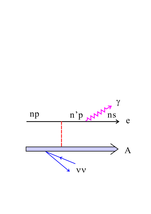
Figure 1: RENP diagrams 1 for alkali atoms. Red dashed line is for Coulomb interaction between valence electron and nucleus.

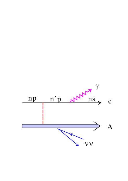
Figure 2: RENP diagrams 2 for alkali atoms.

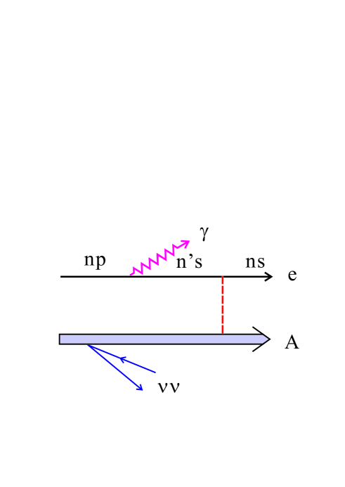
Figure 3: RENP diagrams 3 for alkali atoms.

RENP spectrum formula for alkali atomic transition $|n^{\prime}p\rangle\rightarrow|ns\rangle+\gamma+\nu\nu\,,n^{\prime}=n+1$ is given by

$$\Gamma_{\gamma 2\nu}(\omega;\,t)=\Gamma_{0}F^{2}(\omega)I(\omega)\eta_{\omega}(t)\,,\hskip 14.22636pt\Gamma_{0}=\frac{3}{4}G_{F}^{2}n^{3}V\epsilon_{eg}\,,$$ (18)

$$F(\omega)=\frac{Q_{w}J_{N}(\epsilon(n^{\prime}p)-\epsilon(ns))}{\epsilon(n^{\prime}p)-\epsilon(np)}\frac{1}{\sqrt{3\pi}}\frac{d_{n^{\prime}pns}}{(\epsilon(n^{\prime}p)-\epsilon(np)+\omega)(\epsilon(np)-\epsilon(ns)-\omega)}\,,\hskip 14.22636ptd_{ab}=\sqrt{3\pi\frac{\gamma_{ab}}{(\epsilon_{a}-\epsilon_{b})^{3}}}\,,$$ (19)

$$I(\omega)=\sum_{i}\Delta_{i}(\omega)I_{i}(\omega)\theta(\omega_{ii}-\omega)\,,\hskip 14.22636pt\omega_{ii}=\frac{\epsilon_{eg}}{2}-\frac{2m_{i}^{2}}{\epsilon_{eg}}\,,$$ (20)

$$I_{i}(\omega)=\frac{\omega^{2}}{3}+\frac{2m_{i}^{2}\omega^{2}}{3\epsilon_{eg}(\epsilon_{eg}-2\omega)}+m_{i}^{2}(1+\delta_{M})\,,\hskip 14.22636pt\Delta_{i}(\omega)=\left(1-\frac{4m_{i}^{2}}{\epsilon_{eg}(\epsilon_{eg}-2\omega)}\right)^{1/2}\,,$$ (21)

with $\delta_{M}=1$ for the Majorana case and zero for the Dirac case. The relation between transition dipole $d_{ab}$ and transition rate $\gamma_{ab}$ (A-coefficient) has been used.

The photon energy spectrum from RENP is continuous below a threshold slightly below the half of the energy difference of initial and final states, $\epsilon_{eg}/2-2m_{0}^{2}/\epsilon_{eg}$ with $m_{0}$ the smallest neutrino mass, hence is separated from the familiar D1 line of alkali atoms at $\epsilon_{eg}$. The spontaneous (and not macro-coherent) emission spectrum of two-photon decay $|e\rangle\rightarrow|g\rangle+\gamma+\gamma$ is continuous starting from $\epsilon_{eg}/2$, but has negligible rates.

The overall rate scale is given by $\Gamma_{0}$, which has the dimension of mass, or $s^{-1}$, in our natural unit of $\hbar=c=1$. Numerically, this value is

$$\Gamma_{0}\sim 54{\rm mHz}\frac{\epsilon_{eg}}{{\rm eV}}(\frac{n}{10^{21}{\rm cm}^{-3}})^{3}\frac{V}{10^{2}{\rm cm}^{3}}(\frac{100{\rm MHz}}{{\rm eV}^{3}})^{-1}\,.$$ (22)

As a reference parameter set, we took a target number density $n=10^{21}$cm^-3, a target volume $V=10^{2}$cm³, A-coefficients, $\gamma_{ab}$’s, in 100 MHz unit, and an available energy $\epsilon_{eg}=1$eV, along with all energies in the eV unit. The rate dependence on these parameters is as explicitly indicated in this equation.

The spectral shape given by this formula is substantially different from the case of valence RENP in the preceding works of the spin current [5], in particular in the low energy limit $\omega\rightarrow 0$. The reason for this is in the nuclear mono-pole current in the neutrino emission vertex, different from the spin current in the valence RENP. Calculation leading to the spectral rate $I(\omega)$ is sketched in Appendix.

The factor $\eta_{\omega}(t)$ is the extractable fraction of field intensity $\epsilon_{eg}n$ stored in the initial upper level $|e\rangle$. The storage and development of target polarization is induced by two trigger laser irradiation of $\omega+\omega^{\prime}=\epsilon(n^{\prime}p)-\epsilon(ns),\omega<\omega^{\prime}$. The storage is due to a second order QED process, for instance M1$\times$E1 type of two-photon paired super-radiance (PSR) via virtual intermediate state $n^{\prime}p_{1/2}\rightarrow n^{\prime}p_{3/2}\rightarrow ns_{1/2}$ in alkali atoms. The calculation of $\eta_{\omega}(t)$ requires numerical solution of the master equation for developing fields and target polarization given in [6], [5]. Usually, $\eta_{\omega}(t)$ is much less than unity, and depends on experimental conditions. In the present work we use a conservative value of $\eta_{\omega}(t)$ in the range $10^{-6}$ [13]. The macro-coherent development of field at frequency $\omega$ and macroscopic polarization between $n^{\prime}p$ and $ns$ up to several to 10 nano-second time range is a prerequisite for experimental success of RENP. The macro-coherence is expected to decay after the phase relaxation time $T_{2}$.

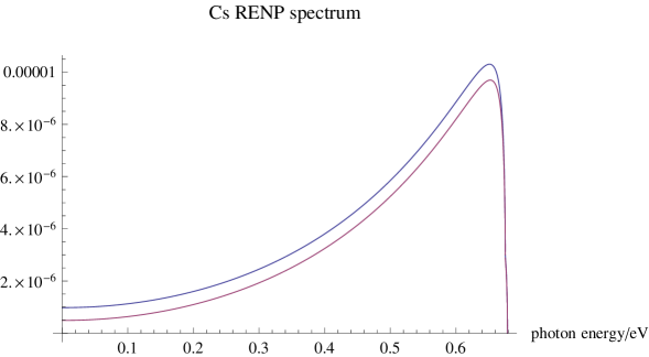
Figure 4: Cs RENP spectrum from de-excitation of energy level at $6P_{1/2}(1.3859{\rm eV})$, assuming the smallest neutrino mass of 0.1 eV in the normal hierarchical (NH) mass pattern, the Majorana case in blue and the Dirac case in magenda, taking other masses and mixing angles consistent with neutrino oscillation experiments. The actual Cs RENP rate is obtained by multiplying $1.5\times 10^{5}(n/10^{21}{\rm cm}^{-3})^{3}(V/10^{2}{\rm cm}^{3})(\eta_{\omega}(t)/10^{-6})$Hz

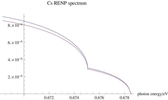
Figure 5: Threshold region corresponding to Fig(4)

In Fig(4) and Fig(5) we plot the spectral shape for ¹³³Cs. Cs data used are states $|e\rangle=6P_{1/2}(1.3859{\rm eV})\,,|g\rangle=6S_{1/2}(0)$ and A-coefficient $7.93\times 10^{5}$s^-1 for $7P_{1/2}(2.6986)\rightarrow 6S_{1/2}$, taken from NIST [15]. For the smallest neutrino mass as large as 0.1 eV as in this example the Majorana vs Dirac distinction is possible by Cs RENP, but for smaller mass values it becomes difficult requiring a large statistic data of RENP. The situation for MD distinction is improved for smaller atomic spacings [14].

For another example we take Xe atomic de-excitation from 6s³P₁ transition. This is an electron-hole system consisting of a valence electron of 6s, 7s,6p and a hole of 5p, much like two valence electron system. We shall use a different scheme from that considered in [5], to utilize the nuclear mono-pole contribution. Data used are energy levels of 6s³P₁(8.437 eV) for initial state, and 7s³P₁(10.593 eV), and its A-coefficient, $\gamma_{7s5p}=8.51\times 10^{7}$s^-1. ¹³¹Xe RENP rate from nuclear pair emission is given by

$$\Gamma_{\gamma 2\nu}(\omega;\,t)=\Gamma_{0}F_{X}^{2}(\omega)I(\omega)\eta_{\omega}(t)\,,\hskip 14.22636ptF_{X}(\omega)=\frac{Q_{w}J_{N}(\epsilon_{7s}-\epsilon_{6s})}{\epsilon_{7s}-\epsilon_{5p}}\frac{1}{\sqrt{3\pi}}\frac{d_{7s5p}}{(\epsilon_{7s}-\epsilon_{6s}+\omega)(\epsilon_{6s}-\epsilon_{5p}-\omega)}\,.$$ (23)

Abbreviated notations are used, paying attention to single electron transitions: for instance $7s$ here means the atomic state $5p^{5}7s$ and $5p$ is an orbital in the closed shell $5p^{6}$ with $\epsilon_{5p}=0$ by definition of the energy origin.

Its spectral shape is given in Fig(6), which shows that neutrino mass differences of this size and different hierarchical mass patterns can be differentiated. MD distinction is impossible with assumed neutrino masses. Although the RENP rate is much smaller due to the assumed atom density appropriate for gas target, the gas target has a number of merits compared with solid targets such as a larger phase relaxation time $T_{2}$.

Figure 6: Xe spectral shape for Dirac and Majorana RENP. Actual rate should be multiplied by $\sim 4\times 10^{3}$Hz for Xe gas density of $7\times 10^{19}$cm^-3, volume $10^{2}$cm³, and $\eta_{\omega}=10^{-6}$. Assumed smallest neutrino masses are 50, 100 meV for the normal (NH) and inverted hierarchical (IH) patterns. NH 50 meV is depicted in blue, IH 50 meV in magenda, NH 100 meV in brown, and IH 100 meV in green. Majorana and Dirac cases are degenerate with this resolution.

VI Summary

We have presented a new enhancement mechanism of RENP due to the mono-pole vertex of neutrino pair emission from inner core electrons and nucleus in heavy atoms. The enhancement factor for RENP rates is very large, depending on the atomic number $\propto Z^{8/3}$ for pair emission from core electrons and $\propto Q_{w}Z^{8/3}$ for pair emission from nucleus where $Q_{w}\sim N-0.044Z$ is the electroweak neutral charge of nucleus. Both rates and spectral shapes of emitted photon energy have been calculated and examples of Cs and Xe RENP have been provided. The new mechanism of mono-pole current opens a variety of possibilities in selection of ideal RENP targets.

VII Appendix: Coulomb integral in Thomas-Fermi model

In the Thomas-Fermi model [11] one assumes the degenerate Fermi gas of electrons at each local point of atom, and relates the Fermi momentum to the number density. The kinetic energy at the Fermi momentum is balanced to the potential energy exerted to electron. In another word, the pressure gradient of degenerate gas is balanced against the electrostatic potential. This gives a relation of the electron number density $n_{e}(r)$ to the potential $\varphi(r)$:

$$\frac{(3\pi^{2}n_{e}(r))^{2/3}}{2m_{e}}-e\varphi(r)=0\,.$$ (24)

The spherical symmetry is assumed.

The second important equation is the Poisson equation, relating the electron number density to the potential. Combined with the density-potential relation above, one arrives at a self-consistent equation for the potential

$$\frac{1}{r}\frac{d^{2}}{dr^{2}}(r\varphi)=\frac{e}{3\pi^{2}}(2m_{e}e\varphi)^{3/2}\,.$$ (25)

It is convenient to introduce dimensionless units of

$$\chi=\frac{4\pi}{Ze}r\varphi\,,\hskip 14.22636ptr=bx$$ (26)

$$b=\frac{(3\pi)^{2/3}}{2^{7/3}}\frac{Z^{-1/3}}{\alpha m_{e}}\sim 0.8853Z^{-1/3}a_{B}\,.$$ (27)

The Thomas-Fermi equation is written for $\chi(x)$;

$$x^{1/2}\frac{d^{2}\chi}{d^{2}x}=\chi^{3/2}\,.$$ (28)

The asymptotic behavior with $x\rightarrow\infty$ is worked out, to give $\chi(x)\rightarrow 144/x^{3}$. The boundary condition at the origin is set from the physical setup, the nuclear charge, which dictates $\chi(x)\rightarrow 1$ as $x\rightarrow 0$, along with $\chi^{\prime}(0)=0$. The problem thus becomes an eigen-value problem. The eigen-function satisfies $\chi(x)=1-c_{1}x+\cdots,c_{1}\sim 1.588$ as $x\rightarrow 0$ [11]. The electron number density is given by

$$n_{e}=\frac{32}{9\pi^{3}}Z^{2}(\alpha m_{e})^{3}(\frac{\chi}{x})^{3/2}\,.$$ (29)

The Coulomb interaction between a valence electron and all core electrons in the closed shell is given by

$$\int d^{3}r_{1}d^{3}r_{2}|\psi_{n}(\vec{r}_{1})|^{2}n_{e}(\vec{r}_{2})\frac{\alpha}{|\vec{r}_{1}-\vec{r}_{2}|}\equiv J_{C}\,.$$ (30)

We may assume that dependence of this quantity on the quantum number of valence electron $n$ is weak and define the Coulomb integral as $\alpha J$. This quantity is given in dimensionless units,

$$J_{C}=\frac{(4\pi)^{2}}{(6\pi^{4})^{2/3}}Z^{4/3}\frac{1}{2}\alpha^{2}m_{e}{\cal J}\sim 31{\rm eV}Z^{4/3}{\cal J}\,,$$ (31)

$${\cal J}=\int_{0}^{\infty}dx_{1}x_{1}^{-1/2}\left(\chi(x_{1})\right)^{3/2}\int_{0}^{x_{1}}dx_{2}x_{2}^{1/2}\left(\chi(x_{2})\right)^{3/2}\,.$$ (32)

Value of ${\cal J}\sim 0.23$ is obtained by numerically solving Thomas-Fermi equation and by integrating results, to give

$$(J_{C})^{2}\sim 50Z^{8/3}{\rm eV}^{2}\,.$$ (33)

Another important integral used in the text is the Coulomb integral between valence electron and nucleus, which is

$$Z\alpha\int d^{3}r_{1}d^{3}r_{2}\frac{|\psi_{N}(\vec{r}_{2})|^{2}n_{e}(\vec{r}_{1})}{|\vec{r}_{1}-\vec{r}_{2}|}\sim\alpha\int d^{3}r\frac{n_{e}(r)}{r}\,,$$ (34)

in the small nucleus limit. Estimate of this quantity in the Thomas-Fermi model is

$$\frac{2^{7/3}}{(3\pi)^{2/3}}Z^{4/3}\alpha^{2}m_{e}\int_{0}^{\infty}dx\frac{\chi(x)^{3/2}}{x^{1/2}}\sim 31{\rm eV}Z^{4/3}\,.$$ (35)

VIII Appendix: Phase space integral over neutrino momenta

We start from two neutrino emission vertex (5), its square to be multiplied by E1 photon emission factor $(\vec{e}\cdot\vec{E})^{2}$ from valence electron and by the Coulomb factor $F$ of eq.(LABEL:coulomb_factor) for rates. Here we concentrate on summation over helicities and momenta of two emitted neutrinos.

Using the helicity summation formula of [4],

$$\sum_{h_{i}}|j_{\nu}\cdot j^{e,q}A|^{2}=\frac{1}{2}(1+\frac{\vec{p}_{1}\cdot\vec{p}_{2}}{E_{1}E_{2}}+\delta_{M}\frac{m_{1}m_{2}}{E_{1}E_{2}})j_{0}^{e,q}(j_{0}^{e,q})^{\dagger}|A|^{2}+\cdots\,,$$ (36)

where $j_{0}^{e,q}$ is the zero-th component electron current, either of electron or of quark, and $(E_{i},\vec{p}_{i})$ are neutrino 4-momenta. The function $A$ refers to all the rest of amplitudes including QED vertex, energy denominators, and all coupling constants. In previous works on valence RENP, the 3-vector part $\propto\vec{j}_{e}$ of electron current (spin-current),

$$\sum_{h_{i}}|j_{\nu}\cdot j^{e}A|^{2}=\frac{1}{2}(1-\frac{\vec{p}_{1}\cdot\vec{p}_{2}}{E_{1}E_{2}}-\delta_{M}\frac{m_{1}m_{2}}{E_{1}E_{2}})\vec{j}_{e}\cdot\vec{j}_{e}^{\dagger}|A|^{2}+\frac{\vec{p}_{1}\cdot\vec{j}^{e}\vec{p}_{2}\cdot\vec{j}^{e}|A|^{2}}{E_{1}E_{2}}+\cdots\,,$$ (37)

has been relevant. Difference of the sign $\pm\frac{\vec{p}_{1}\cdot\vec{p}_{2}}{E_{1}E_{2}}$ appears in the suppressed region of the spectrum: for the mono-pole current (36) the low energy limit $\omega\sim 0$ neutrino momenta are nearly balanced, $\vec{p}_{1}\sim-\vec{p}_{2}$, and there is a more suppression in the low energy limit for the mono-pole case. In eqs.(36) and .(37) we neglected possibly time reversal odd terms.

In the phase space integral of neutrino momenta,

$$\int\frac{d^{3}p_{1}d^{3}p_{2}}{(2\pi)^{2}}\delta(E_{1}+E_{2}+\omega-\epsilon_{eg})\delta(\vec{p}_{1}+\vec{p}_{2}+\vec{k})(\cdots)$$ (38)

one of the momentum integration is used to eliminate the delta function of the momentum conservation. The resulting energy-conservation is used to fix the relative angle factor $\cos\theta$ between the photon and the remaining neutrino momenta, $\vec{p}_{1}\cdot\vec{k}=p_{1}\omega\cos\theta$. Noting the Jacobian factor $E_{2}/p\omega$ from the variable change to the cosine angle, one obtains one dimensional integral over the neutrino energy $E_{1}$:

$$I_{ij}(\omega)\frac{\Delta_{ij}(\omega)}{2\pi}\equiv\frac{1}{2\pi\omega}\int_{E_{-}}^{E_{+}}dE_{1}E_{1}E_{2}\frac{1}{2}(1+\frac{\vec{p}_{1}\cdot\vec{p}_{2}}{E_{1}E_{2}}+\delta_{M}\frac{m_{1}m_{2}}{E_{1}E_{2}})\,,\hskip 14.22636ptE_{2}=\epsilon_{eg}-\omega-E_{1}\,.$$ (39)

The angle factor constraint $|\cos\theta|\leq 1$ places a constraint on the range of neutrino energy integration,

$$E_{\pm}=\frac{1}{2}\left((\epsilon_{eg}-\omega)(1+\frac{m_{i}^{2}-m_{j}^{2}}{\epsilon_{eg}(\epsilon_{eg}-2\omega)})\pm\omega\Delta_{ij}(\omega)\right)\,,$$ (40)

$$\Delta_{ij}(\omega)=\left\{\left(1-\frac{(m_{i}+m_{j})^{2}}{\epsilon_{eg}(\epsilon_{eg}-2\omega)}\right)\left(1-\frac{(m_{i}-m_{j})^{2}}{\epsilon_{eg}(\epsilon_{eg}-2\omega)}\right)\right\}^{1/2}\,.$$ (41)

The integrand is a quadratic function of neutrino energy [14], and it is easily integrated to give

$$I_{ij}(\omega)=\frac{\omega^{2}}{3}+\frac{1}{2}(m_{i}^{2}+m_{j}^{2})+\frac{1}{3}\frac{\omega^{2}(m_{i}^{2}+m_{j}^{2})}{\epsilon_{eg}(\epsilon_{eg}-2\omega)}-\frac{3}{4}\frac{(\epsilon_{eg}-\omega)^{2}}{\epsilon_{eg}^{2}(\epsilon_{eg}-2\omega)^{2}}(m_{i}^{2}-m_{j}^{2})^{2}+\delta_{M}m_{i}m_{j}\,.$$ (42)

The result, eq.(21) and in other places of the text, $I_{i}(\omega)=I_{ii}(\omega)$ is needed.

Acknowledgements    We appreciate M. Tanaka for a discussion. This research was partially supported by Grant-in-Aid for Scientific Research on Innovative Areas ”Extreme quantum world opened up by atoms” (21104002) from the Ministry of Education, Culture, Sports, Science, and Technology.

References

[1]
G. L. Fogli, E. Lisi, A. Marrone, D. Montanino, A. Palazzo, and A. M. Rotunno,
Phys. Rev.D 86, 013012 (2012).
M. C. Gonzalez-Garcia, Michele Maltoni, Jordi Salvado, Thomas Schwetz,
Journal of High Energy PhysicsDecember 2012, 123.
D. V. Forero, M. Toacutertola, and J. W. F. Valle,
Phys. Rev.D 86, 073012 (2012).
[2]
G. Drexlin, V. Hannen, S. Mertens, and C. Weinheimer, Current Direct
Neutrino Mass Experiments,
Advances in High Energy Physics Volume 2013 (2013)Article ID 293986.
[3]
A. Gando et al,
Phys. Rev. Lett.110, 062502 (2013), and
arXiv:1201.4664v2[hep-ex] (2012).
M.Auger et al,
Phys. Rev. Lett.109, 032505 (2012).
[4]
M. Yoshimura, Phys. Rev.D75.
113007 (2007).
[5]
A. Fukumi et al.,
Progr. Theor. Exp. Phys.2012, 04D002;
arXiv1211.4904v1[hep-ph](2012), and
and references cited therein.
[6]
M. Yoshimura, N. Sasao, and M. Tanaka,
Phys. RevA86,013812(2012),
and
Dynamics of paired superradiance,
arXiv:1203.5394[quan-ph] (2012).
[7]
M.A. Bouchiat and C. Bouchiat,
J. Phys. (Paris)35, 899 (1974).
[8]
M.A. Bouchiat et al,
Phys. Lett.134B, 463(1984),
and references therein.
[9]
P.S. Drell and E.D. Commins,
Phys. Rev.A 32, 2196(1985),
and references therein.
[10]
M.C. Noecker, B.P. Materson, and C.E. Wieman,
Phys. Rev. Lett.61, 310 (1988),
and references therein.
[11]
B.H. Bransden and C.J. Joachain,
Physics of Atoms and Molecules,
Chapter 8.3, 2nd edition, Prentice Hall(2003).
[12]
D. Neuffer and E.D. Commins,
Phys. Rev. A16,844(1977).
[13]
In [5] a result for
numerical simulation of
is presented for pH2 molecule target
(strong source of paired super-radiance (PSR)
of E1 E1 transition, and see
Fig 14 of this reference for time dependence).
Its time dependence is complicated:
a fast rise in ns), then a plateau region
of magnitude of duration of
several nano-seconds, finally gradual decrease
ending around at 12 ns (end time of calculation).
For RENP rate calculations,
numerical simulations based on the master
equation given in [5] should be
performed for weaker PSR process of
specific targets considered,
which is expected to give different time
profile and larger values of .
[14]
D.N. Dinh, S. Petcov, N. Sasao, M. Tanaka,
and M. Yoshimura,
Phys. Lett.B719,154(2012), and
arXiv1209.4808v1[hep-ph].
[15]
National Institute of Standards and Technology (NIST) Atomic Spectra
Database: see http://www.nist.gov