Minkowski structure for purity and entanglement of Gaussian bipartite states

Abstract

The relation between the symplectic and Lorentz groups is explored to investigate entanglement features in a two-mode bipartite Gaussian state. We verify that the correlation matrix of arbitrary Gaussian states can be associated to a hyperbolic space with a Minkowski metric, which is divided in two regions - separablelike, and entangledlike, in equivalence to timelike and spacelike in special relativity. This correspondence naturally allows the definition of two insightful invariant squared distances measures - one related to the purity and another related to amount of entanglement. The second distance allows us to define a measure for entanglement in terms of the invariant interval between the given state and its closest separable state, given in a natural manner without the requirement of a minimization procedure.

Introduction. The symplectic group is isomorphic to the structure of the Lorentz and de Sitter groups, as was firstly pointed out by Dirac himself in his famous 3 + 2 de Sitter group article Dirac . In fact, all Gaussian light field states embody the symplectic structure kim , as has been explored in the implementation of several features such as quadrature squeezing and quantum entanglement. A particularly important separability criterion, based on the symplectic structure of Gaussian states (GS), was given by Simon simon , as an extension for continuous variables of the Peres-Horodecki positivity under partial transposition (PPT) criterion peres ; horodecki . It is remarkable that positive maps can actually be associated to a hyperbolic geometry displaying formal similarity with the spacetime manifold of special relativity. This connection was reported earlier hss1 ; hss2 for two-qubit systems where the concept of hyperbolic squared distance was introduced as a measure of entanglement, within a compact support in contrast with the space-time manyfold. The relation of the invariants of the Lorentz group, namely space-time squared intervals, with transformations and entanglement properties of GS seems to us quite advantageous to be seen from a geometric perspective.

In this paper we give a geometrical picture of the separability bound for two-mode bipartite GS in terms of a hyperbolic geometry having a Minkowski metric, and explore the formal similarities between purity and entanglement properties with some familiar concepts in theory of relativity. The advantage of such an approach is made clear for the definition of distances related to entanglement and purity measures in terms of invariant intervals, which do not rely on some optimization procedure as usual paulina2 ; vedral . We exemplify by comparing the distance based measure of entanglement to other well known measures of entanglement for symmetric and non-symmetric Gaussian states produced by sending a two-mode thermal state through lossy optical fibers.

Gaussian states. Gaussians continuous variables states are standard in quantum mechanics, whose information is stored in two simple quantities: the Mean Value Vector and the Covariance Matrix (CM) englert2 . Mean values can be displaced by local operations to the null vector, without affecting entanglement, being usually neglected. For a bipartite system described by bosonic operators, $(a_{1},a_{2})$, the $4\times 4$ CM reads, after suitable local operations, as simon

$${\bf V}=\left(\begin{array}[]{cc}{\bf V}_{1}&\bf C\\ {\bf C}^{\dagger}&{\bf V}_{2}\end{array}\right),\,\,{\bf V}_{i}=n_{i}\mathbf{I},\,\,{\bf C}=\left(\begin{array}[]{cc}m_{s}&m_{c}\\ m_{c}&m_{s}\end{array}\right),$$ (1)

$n_{i},m_{c},m_{s}\in\mathbb{R}$, being hermitian and positive semidefinite, $\textbf{V}^{\dagger}=\textbf{V}\geq 0$. Additionally, the non-commutativity of the creation/annihilation operators, imposes a constraint on V:

$${\bf V}+\frac{1}{2}{\bf E}\geq 0,$$ (2)

where ${\bf E}=\text{diag}(\mathbf{Z},\mathbf{Z})$, ${\bm{Z}}=\text{diag}(1,-1)$. Separable Gaussian bipartite states must also obey simon

$${\bf\widetilde{V}}+\frac{1}{2}{\bf E}\geq 0,$$ (3)

where ${\bf\widetilde{V}}={\bf TVT}$ is achieved by a partial phase space mirror reflection, ${\bf T}=\text{diag}({\bf I},{\bf X})$, and ${\bf X}=\text{adiag}(1,1)$. It is known that a necessary and sufficient condition for the positivity semi-definiteness of a matrix is that its upper left block be positive definite and the block’s Schur complement be positive semidefinite. Thus the physical positivity criterion (2) applies if and only if mcol1

$${{\bf V}_{1}}+\tfrac{1}{2}{\bf Z}>0\,\,\,\,\,\,\text{and}\,\,\,\,\,\,\mathcal{S}({\bf V}+\tfrac{1}{2}{\bf E})\geq 0,$$ (4)

and the separability condition (3) holds only if mcol1

$${{\bf V}_{1}}+\tfrac{1}{2}{\bf Z}>0\,\,\,\,\,\,\text{and}\,\,\,\,\,\,\mathcal{S}({\widetilde{\bf V}}+\tfrac{1}{2}{\bf E})\geq 0.$$ (5)

Geometry. In order to explore the geometric features of the GS we first write the inequalities in (4) and (5) in terms of the matrices entries in (1). We verify that the inequalities in (4) reduce to the quadratic form

$$\delta s^{2}=\delta t^{2}-\delta x^{2}-\delta y^{2}\geq 0,$$ (6)

having a Minkowski metric, where

$$\delta{t}^{2} = (I_{1}-\tfrac{1}{4})^{-1}\left(I_{1}-\tfrac{1}{4}-\tfrac{1}{2}I_{4}/I_{2}\right)^{2}I_{2},$$

$$\delta{x}^{2} = (I_{1}-\tfrac{1}{4})^{-1}\left(\tfrac{1}{4}I_{4}^{2}/I_{2}-I_{1}I_{3}^{2}\right),$$

$$\delta{y}^{2} = \tfrac{1}{4}(I_{1}-\tfrac{1}{4})^{-1}\left(I_{1}-\tfrac{1}{4}+I_{3}\right)^{2},$$ (7)

with the local invariants simon being $I_{1}=\det\mathbf{V}_{1}$, $I_{2}=\det\mathbf{V}_{2}$, $I_{3}=\det\mathbf{C}$, and $I_{4}=\text{tr}(\mathbf{V}_{1}\mathbf{Z}\mathbf{C}\mathbf{Z}\mathbf{V}_{2}\mathbf{Z}\mathbf{C^{\dagger}}\mathbf{Z})$. In this $1+2$ dimensional space, a separatrix is defined by $\delta s^{2}=0$ setting the boundary for discerning physical from nonphysical states. States lying at the boundary are pure bipartite GS, corresponding to equality in (4). By computing all the terms in (6) we get

$$\delta s^{2}=\det{\bf V}-\tfrac{1}{4}\sigma_{{\bf V}}+\tfrac{1}{16},$$ (8)

where $\det{\bf V}=I_{1}I_{2}+I_{3}^{2}-I_{4}$ and $\sigma_{{\bf V}}=I_{1}+I_{2}+2I_{3}$ serafini . An arbitrary pure global state is characterized by $\det{\bf V}=1/16$ and $\sigma_{{\bf V}}=1/2$, and so $\delta s^{2}=0$ and is located at the external conic boundary, defining an isosurface for states with unit purity $\mathcal{P}=\rm{Tr}(\rho^{2})=1$ (See Fig. 1). Conic isosurfaces inside the volume define states with same purity, $\mathcal{P}=1/(4\sqrt{\det{\bf V}})$. Therefore, analogously to intervals in the space-time, defined as the distance between two points (events) in the light-cone, an interval here connects a given state with a certain purity $\mathcal{P}<1$ to its closest pure state situated at the external surface of the physical cone of existence $\mathcal{P}=1$. Since both purity $\mathcal{P}$ and $\sigma_{{\bf V}}$ (the seralian) are preserved by unitary operations, all states lying in a $\mathcal{P}$ isosurface are connected by unitary operations. So the Lorentz invariance of $\delta s^{2}$ is associated to invariance of $\mathcal{P}$ under an arbitrary unitary operation, where ${\bf V^{\prime}}={\bf S}^{\dagger}{\bf V}{\bf S}$ is the CM under a symplectic transform ${\bf S}$ over ${\bf V}$, related to the arbitrary unitary operation $U$ by $U{\bf v}U^{-1}={\bf S}{\bf v}$: ${\bf v}=(a_{1}^{\dagger},a_{1},a_{2}^{\dagger},a_{2})^{\dagger}$.

In relativity the causal structure allows that at any event another light-cone be defined, therefore restricting all world lines. For the GS depicted in a hyperbolic space (Minkowski picture), the $\mathcal{P}=1$ cone defines all states that can be generated from the vacuum (as all GS can be generated by convenient Gaussian operations over the vacuum). Trace preserving operations may preserve purity (if unitary) or decrease it (if not unitary). Being at a certain state of the cone of existence, a new set of Gaussian operations lead to any new state inside the cone if non-unitary trace preserving operations are allowed. While local unitary operations must connect states in a specific conic isosurface, arbitrary (trace preserving) non-unitary operations, can move states from the surface to any state inside the cone volume, which in that case preserves (or decreases) the amount of entanglement depending on the nature of the operation. Here, similarly to the limiting velocity of light in relativity, the purity $\mathcal{P}=1$ is the limiting quantity.

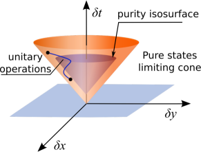
Figure 1: (Color Online) Universe cone for any two-mode bipartite GS. Unitary operations connect any two-states with same purity lying in a conic isosurface of purity.

The squared distance for entanglement. Global operations can certainly change the amount of entanglement of a given state, transforming from one state to another with a different amount of entanglement. However local (non-stochastic) operations cannot change it, while they certainly change the state. So local operations form a special class of causal operations connecting states with the same amount of entanglement. Let us discuss this point with an appropriate picture, rewriting the inequalities in (5) as

$$\delta\tilde{s}^{2}=\delta{t}^{2}-\delta{x}^{2}-\delta\tilde{y}^{2}\geq 0$$ (9)

with

$$\delta\tilde{y}^{2} = \tfrac{1}{4}\left(I_{1}-\tfrac{1}{4}\right)^{-1}\left(I_{1}-\tfrac{1}{4}-I_{3}\right)^{2}.$$ (10)

An entangled GS necessarily implies $I_{3}<0$ simon . Therefore Eq. (9) turns out to be the Simon simon separability criteria for GS. So the Minkowski structure emerges with a separatrix given by $\delta\tilde{s}^{2}=0$, dividing the space into separable-like and entangled-like regions. $\delta\tilde{s}^{2}\geq 0$ includes all separable states, while $\delta\tilde{s}^{2}<0$ corresponds to all entangled GS.

We must understand the meaning of such a relation between both regions, and for that we address to Fig. 2. The Minkowski space deals with intervals (between events), while the symplectic deals with states. Again we match these two features by identifying the meaning of the invariant squared distance interval in (9).

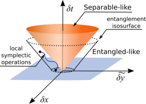
Figure 2: (Color Online) Separation between the separable-like and entangled-like regions after partial transposition of a two-mode bipartite state. Any two states lying at a conic entanglement isosurface can be connected through local ${\rm Sp}(2,\mathbb{R})\otimes{\rm Sp}(2,\mathbb{R})$ operations, and therefore have the same amount of entanglement.

The interval defined in the hyperbolic space is actually a distance between the given state and the closest separable state lying at the separatrix. Since entanglement does not change due to local unitary operations, the two regions are disconnected by any ${\rm Sp}(2,\mathbb{R})\otimes{\rm Sp}(2,\mathbb{R})$ unitary operation. In fact only points in the Minkowski space which have the same entanglement can be connected by those operations. Therefore any two states with the same amount of entanglement belong to the same conic isosurface. The Lorentz invariance of $\delta\tilde{s}^{2}$ is associated to the invariance of entanglement of two-mode bipartite GS under arbitrary local symplectic unitary operations, i.e., for ${\bf V^{\prime}}={\bf S_{L}}^{\dagger}{\bf V}{\bf S_{L}}$, where ${\bf S_{L}}$ must be

$$U_{L}{\bf v}U^{-1}_{L}={\bf S_{L}}{\bf v},\;\;\;{\bf S_{L}}=\text{diag}({\bf S_{1}},{\bf S_{2}}),$$ (11)

with the condition ${\bf S_{L}}^{\!\!\!-1}={\bf ES_{L}}^{\!\!\dagger}{\bf E}$. In a simplified scenario, any state living on the $(y,t)$ plane is linked to other states with constant $\delta{t}$ by a rotation in the $(x,y)$ plane. At that plane, violating inequality (9) means that the state lies on a line parallel to the cone’s surface: $\delta{\tilde{t}}^{2}-\delta{\tilde{y}}^{2}=-\delta\tilde{s}^{2}$. Since all states with the same $\delta\tilde{s}^{2}$ are equidistant to the separatrix they are connected through operations in (11) lying in a straight line parallel to the separability boundary, $\delta{\tilde{t}}^{2}=\delta{\tilde{y}}^{2}$, as in Fig. 2.

Entanglement properties and quantification. Now, we investigate the quality of $|\delta\tilde{s}^{2}|$ as a good measure of entanglement, which requires it to satisfy some specific properties zyczkowski in the context of GS and Gaussian operations GiedkeCirac ; fiurasec . It will be useful for us rewrite eq. (9) as

$$\delta\tilde{s}^{2}=\det\left({\bf\widetilde{V}}+\tfrac{1}{2}{\bf E}\right)=(\tilde{n}_{+}^{2}-1/4)(\tilde{n}_{-}^{2}-1/4),$$ (12)

where $\tilde{n}_{\pm}$ are the symplectic eigenvalues of $\tilde{\bf V}$, explicitly given by serafini

$$\tilde{n}_{\pm}^{2}=\tfrac{I_{1}+I_{2}}{2}-I_{3}\pm\sqrt{\left(\tfrac{I_{1}-I_{2}}{2}\right)^{2}-(I_{1}+I_{2})I_{3}+I_{4}}.$$ (13)

Furthermore, $\tilde{\bf V}$ is positive semidefinite and $\tilde{n}_{+}\geq\tilde{n}_{-}\geq 1/2$ for a separable state, while for an entangled state $0<\tilde{n}_{-}<1/2$ fulfilling $\delta\tilde{s}^{2}<0$ (in analogy to the space-like condition in relativity). Eqs. (12) and (13) link the squared distance $\delta\tilde{s}^{2}$ (when $\delta\tilde{s}^{2}\leq 0$) with the Simon separability criteria for bipartite GS simon expressed as a function of the symplectic eigenvalues. In fact, measuring entanglement by distances in a Hilbert space (see for instance paulina3 ; mcol2 for the Bures metric) requires a hard minimization procedure over a set of separable states. Here instead, $\delta\tilde{s}^{2}$ does not require any minimization procedure since it is given due to the Minkowski structure as a straight line between the two parallel conic surfaces, one containing the given state and the second its closest separable state. Therefore $\delta\tilde{s}^{2}$ satisfy the computability requirement.

The discriminance requirement states that $\delta\tilde{s}^{2}=0$ if and only if $\hat{\rho}$ is separable, and this is true for all bipartite GS, since there is no bipartite GS with bound entanglement werner . Two states living closer inside the existence cone have partial transpositions also close to each other since by construction the difference between the original state and the partially transposed is a sign in $I_{3}$, see eq.(10): this defines the asymptotic continuity for the measure.

Given a convex decomposition of a quantum state, the entanglement of this state cannot be less than the convex sum of the entanglement of each part of the decomposition. Given two arbitrary two-mode bipartite GS, $\hat{\rho}$ and $\hat{\rho}^{\prime}$ with corresponding entanglement $\delta\tilde{s}^{2}$ and $\delta\tilde{s}^{\prime 2}$ then

$$\hat{\rho}=\int\!d^{2}\!\alpha\,d^{2}\!\beta\,\,P(\alpha,\beta)\,\,{\hat{D}}_{\alpha\beta}\,\hat{\rho}^{\prime}{\hat{D}}^{\dagger}_{\alpha\beta}\rightarrow|\delta\tilde{s}^{2}|\leq|\delta\tilde{s}^{\prime 2}|,$$ (14)

where $P$ is a normalized Gaussian probability function with CM $\mathbf{P}$, and ${\hat{D}}_{\alpha\beta}$ is the displacement operator . To prove the necessary condition of convexity, given the CMs of the above relation ${\bf V}={\bf P}+{\bf V^{\prime}}$ we derive that

$$\left|\det\left({\bf\widetilde{V}}+\tfrac{1}{2}{\bf E}\right)\right|\geq\left|\det\left({\bf\widetilde{V}^{\prime}}+\tfrac{1}{2}{\bf E}\right)\right|.$$ (15)

GS entanglement cannot be distilled by LOCC Gaussian operationsfiurasec ; GiedkeCirac . Therefore any good entanglement measure cannot decrease under these operations - a property called monotonicity. To prove the monotonicity for $\delta\tilde{s}^{2}$, first let us note that all stochastic Gaussian LOCC, represented by a $8\times 8$ CM $\Gamma$ acting on a input GS with CM $\bf V$, can be reproduced by means of a deterministic Gaussian LOCC fiurasec , furthermore $\Gamma$ is separable with respect to the input (with CM $\bf V$) and output states (with CM $\bf V^{\prime}$). Under these conditions $\bf V^{\prime}\leq\bf V$ implying necessarily that ${\bf\widetilde{V}^{\prime}}\leq{\bf\widetilde{V}}$ GiedkeCirac . Is is direct to see that $\left|\det\left({\bf\widetilde{V}^{\prime}}+\tfrac{1}{2}{\bf E}\right)\right|\leq\left|\det\left({\bf\widetilde{V}}+\tfrac{1}{2}{\bf E}\right)\right|$. All those properties guarantee that $|\delta\tilde{s}^{2}|$ (when $\delta\tilde{s}^{2}\leq 0$) is an entanglement monotone zyczkowski .

It is interesting to compare the Minkowski interval $\delta\tilde{s}^{2}$ with other available measures of entanglement. For that we define

$${\rm E}(\rho_{12})=f\left(2\sqrt{\frac{\delta\tilde{s}^{2}}{(\tilde{n}_{+}^{2}-1/4)}+\frac{1}{4}}\right),$$ (16)

being $f(x)$ a monotonically decreasing function over the interval $x\in(0,1]$ . In that form Eq. (16) can be connected to two distinct entanglement measures - the Logarithmic Negativity (LN) serafini and the Entanglement of Formation EoF for symmetric GS Gie03 . The LN measure is given by taking $f(x)=-{\rm ln}(x)$ in Eq. (16) For symmetric GS ($I_{1}=I_{2}$), the EoF can be computed analytically Gie03 , and is given by taking $f(x)=c_{+}(x)\log_{2}(c_{+}(x))-c_{-}(x)\log_{2}(c_{-}(x))$ with $c_{\pm}(x)=(x^{-1/2}\pm x^{1/2})^{2}/4$ in Eq. (16). Both the LN and the EoF are monotonically decreasing function of $\tilde{n}_{-}$: the closer $\tilde{n}_{-}$ is to zero, the state is more entangled. There is no closed analytical expression for the EoF for non-symmetrical GS paulina2 , whose computation relies on a minimization procedure wolf . We employ this same formula to calculate a lower bound for the EoF for non-symmetric GS rigolin .

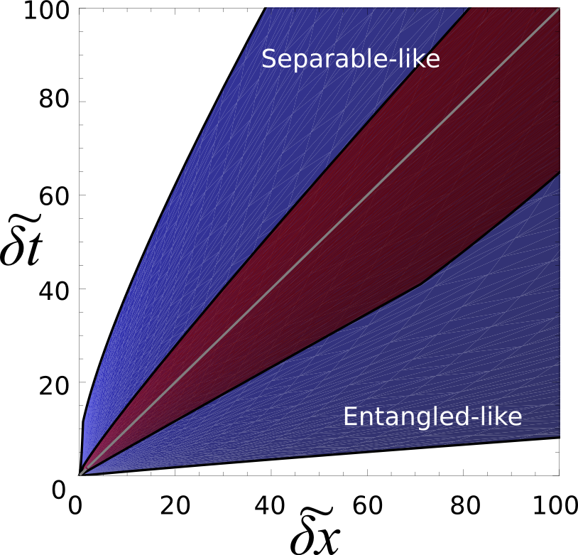
Figure 3: (Color Online) Blue Region: Set of all TMTSS with a fixed dissipative parameter of $d=2.5$ and varying thermal photon number $\bar{n}$ from $0$ to $1.5$, and squeezing rate $r$ from $0$ to $3.0$. The color map in the (blue) limited region indicates from light to darker the increasing feature of $r$. Red Region: Set of all TMTSS above after asymmetric action of a lossy fiber with $\ell=0.5$. The effect of the asymmetry is to constrain the available states to a smaller area around the separatrix.

We now concentrate on the kind of GS actually generated experimentally — the two-mode thermal squeezed state (TMTSS) daffer — produced in a nonlinear crystal with internal noise. These states are characterized by the following values for the parameters: $n\equiv n_{1}=n_{2}=(h_{1}+h_{2})/4$, $m_{s}=0$, and $m_{c}=(h_{1}-h_{2})/4$, with $h_{i}=\left\{e^{-p_{i}}+d\,(2\bar{n}+1)\left[{(1-e^{-p_{i}})}/{p_{i}}\right]\right\}$ and $p_{1}=d+2r$ and $p_{2}=d-2r$. $d$ is a dissipative parameter, and $r$ is the squeezing parameter. $\bar{n}$ is the mean number of thermal photons introduced by the quantum noise. Therefore $\delta{t}^{2}=n^{2}\left(n^{2}-\tfrac{1}{4}-{m_{c}^{2}}\right)^{2}/(n^{2}-\tfrac{1}{4})$, $\delta\tilde{y}^{2}=\tfrac{1}{4}\left(n^{2}-\tfrac{1}{4}+m_{c}^{2}\right)^{2}/(n^{2}-\tfrac{1}{4})$ and $\delta{x}^{2}=0$. The measure (16) turns out to be simply ${\rm E}(\rho_{12})=f\left[2(n-|m_{c}|)\right]$. It vanishes at the separability boundary $m_{c}=\pm(n-1/2)$. Since any ${\rm Sp}(2,\mathbb{R})\otimes{\rm Sp}(2,\mathbb{R})$ unitary operation does not change the amount of entanglement, necessarily all states connected through it are located on lines parallel to the separatrix (see Fig. 3). For a fixed $d=2.5$ as $r$ is increased the state gets more entangled, while by increasing $\bar{n}$ it tends to lie on the separable-like region. Asymmetry effects can be introduced by assuming that the TMTSS is distributed by lossy optical fibers wolf . The fibers output field state will have a CM of the form (1) with $n^{\prime}_{i}\equiv(n_{i}-1/2)T_{i}^{2}+1/2$, for $i=1,2$ and $m^{\prime}_{c}\equiv m_{c}T_{1}T_{2}$. The transmission coefficients in the asymmetric configuration are $T_{1}=1$, $T_{2}=\exp(-\ell)$ , where $\ell$ is a dimensionless length related to the fiber’s absorption. Now $\delta{t}^{2}={n^{\prime}_{2}}^{2}\left({n^{\prime}_{1}}^{2}-\tfrac{1}{4}-\tfrac{n^{\prime}_{1}}{n^{\prime}_{2}}{m^{\prime}_{c}}^{2}\right)^{2}/(n_{1}^{\prime}-\tfrac{1}{4})$, $\delta\tilde{y}^{2}=\tfrac{1}{4}\left({n^{\prime}_{1}}^{2}-1/4+{m^{\prime}_{c}}^{2}\right)^{2}/(n_{1}^{\prime}-\tfrac{1}{4})$, $\delta{x}^{2}=0$ and the separatrix will be at $(n^{\prime}_{1}\pm{1}/{2})(n^{\prime}_{2}\pm{1}/{2})={m^{\prime}_{c}}^{2}$. In Fig. 3, we see that due to the additional noise introduced by the fiber, the states are confined to a region around the separatrix.

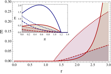
Figure 4: (Color Online) Measuring entanglement of (asymmetric) GS living in the red region of Fig.3 using the Minkowski Distance $|\delta s^{2}|/2000$ (continuous lines), the EoF bound (dashed lines) and the LN (dotted line) as a function of $r$ with fixed $d=2.5$, $\bar{n}=0.5$ and $\ell=0.5$. In the inset we show the same quantities for a symmetric GS ($\ell=0$) living in the blue region of fig.3 and for the asymmetric GS (shadowed curves) with $\ell=0.5$ living in the red region of fig.3 as a function of the mean thermal number $\bar{n}$ with $r=3$ and $d=2.5$.

To compare the different measures, we plot $|\delta\tilde{s}^{2}|$ in Fig. 4 and the two cases for (16): the EoF bound and the LN when $r$ and $\bar{n}$ increase. The measures given by (16) have qualitatively the same behavior (with the LN being always greater than the EoF bound) for symmetric and asymmetric states. On the other side, $|\delta\tilde{s}^{2}|$ is always greater then both (note that this function is rescaled in Fig.4). As $r$ increases from zero to $r_{0}\approx 1.25$, the noise and dissipation of the crystal are responsible for the separability of the TMTSS. After this threshold the state becomes entangled as can be seen for the three plotted functions. The behavior with $\bar{n}$ variation is shown in the inset and now the measures differ qualitatively: as the functions (16) always decrease, the distance reaches a maximum value and then decreases to zero.

Discussion. We have explored the symplectic and Lorentz groups relation to investigate some formal analogies with special relativity, related to quantum mechanical features of GS as purity and entanglement. Particularly, we have observed that a monotone distance based entanglement measure can be analytically given, being the optimization, usually required for this kind of measure, directly given by the Minkowski structure. We remark that the present description can be generalized to include non-Gaussian states as well. In that situation there are states, which are entangled although satisfying $\delta\tilde{s}^{2}\geq 0$, thus lying within the cone. Those states are not detected by the PPT criterion, and are known as bound entangled states. So, what is mostly interesting in the Minkowski diagram in Fig. 2 is that it then splits the space into a region containing only entanglement that can be distilled (by non-Gaussian operations), and a region containing separable states and entangled states that cannot be distilled by any kind of local operations. Finally we suggest that beyond the clear importance of this picture for entanglement quantification, given high degree of control in the experimental generation Gaussian quantum light fields, one could think of this system as a general analog simulator for relativistic phenomena.

- (1) P.A.M. Dirac, J. Math. Phys. 4, 901 (1963).
- (2) Y.S. Kim and M.E. Noz, Am. J. Phys. 51, 368 (1983).
- (3) R. Simon, Phys. Rev. Lett. 84, 2726 (2000).
- (4) A. Peres, Phys. Rev. Lett. 77, 1413 (1996).
- (5) P. Horodecki, Phys. Lett. A 232, 333 (1997).
- (6) I. Bengtsson, K. Zyczkowski, Geometry Of Quantum States: An Introduction To Quantum Entanglement (Cambridge University Press, UK, 2008).
- (7) H. Braga, S. Souza, and S.S. Mizrahi, Phys. Rev. A 81, 042310 (2010).
- (8) H. Braga, S. Souza, and S.S. Mizrahi, Phys. Rev. A 84, 052324 (2011) .
- (9) V. Vedral and M. B. Plenio, Phys. Rev. A 57, 1619 (1998)
- (10) P. Marian and T. A. Marian, Phys. Rev. Lett. 101, 220403 (2008).
- (11) B.-G. Englert and K. Wódkiewicz, Int. J. Quant. Inf. 1, 153 (2003); J. Eisert and M.B. Plenio, Int. J. Quant. Inf. 1, 479 (2003).
- (12) M.C. de Oliveira, Phys. Rev. A 70, 034303 (2004).
- (13) A. Serafini, F. Illuminati, S. De Siena, J. Phys. B: At. Mol. Opt. Phys. 37, L21 (2004); G. Adesso, A. Serafini, F. Illuminati, Open Sys. Information Dyn. 12, 187 (2005).
- (14) P. Marian, T. A. Marian and H. Scutaru, Phys. Rev. A 68, 062309 (2003).
- (15) M. C. de Oliveira, Phys. Rev. A 72, 012317 (2005).
- (16) G. Giedke, M.M. Wolf, O. Kruger, R.F. Werner, J.I. Cirac, Phys. Rev. Lett. 91, 107901 (2003).
- (17) M.M. Wolf, G. Giedke, O. Kruger, R.F. Werner, J.I. Cirac, Phys. Rev. A 69, 052320 (2004).
- (18) G. Rigolin and C. O.Escobar, Phys. Rev. A 69, 012307 (2004).
- (19) S. Daffer, K. Wódkiewicz, and J.K. McIver, Phys. Rev. A 68, 012104 (2003).
- (20) G. Giedke, J.I. Cirac, Phys. Rev. A 66, 032316 (2002).
- (21) J. Fiurášek, Phys. Rev. Lett. 89, 137904 (2002).
- (22) R.F. Werner and M.M. Wolf, Phys. Rev. Lett. 86, 3658 (2001).