Dynamic Length Scales in Glass-Forming Liquids: A Inhomogeneous Molecular Dynamics Simulation Approach

Abstract

In this work we numerically investigate a new method for the characterization of growing length scales associated with spatially heterogeneous dynamics of glass-forming liquids. This approach, motivated by the formulation of the inhomogeneous mode-coupling theory (IMCT) [Biroli G. et al. Phys. Rev. Lett. 2006 97, 195701], utilizes inhomogeneous molecular dynamics simulations in which the system is perturbed by a spatially modulated external potential. We show that the response of the two-point correlation function to the external field allows one to probe dynamic correlations. We examine the critical properties shown by this function, in particular the associated dynamic correlation length, that is found to be comparable to the one extracted from standardly-employed four-point correlation functions. Our numerical results are in qualitative agreement with IMCT predictions but suggest that one has to take into account fluctuations not included in this mean-field approach in order to reach quantitative agreement. Advantages of our approach over the more conventional one based on four-point correlation functions are discussed.

Current address: Department of Physics, Niigata University, Niigata 950-2181, Japan Institute for Molecular Science] Institute for Molecular Science, Okazaki, Aichi 444-8585, Japan [The Graduate University for Advanced Studies] School of Physical Sciences, The Graduate University for Advanced Studies, Okazaki, Aichi 444-8585, Japan Institute for Molecular Science] Institute for Molecular Science, Okazaki, Aichi 444-8585, Japan [The Graduate University for Advanced Studies] School of Physical Sciences, The Graduate University for Advanced Studies, Okazaki, Aichi 444-8585, Japan Current address: Department of Physics, Nagoya University, Nagoya, Aichi 464-8501, Japan University of Tsukuba] Institute of Physics, University of Tsukuba, Tsukuba 305-8571, Japan CEA Saclay] Institut Physique Théorique, CEA Saclay, 91191 Gif Sur Yvette, France and CNRS URA 2306 Columbia University] Department of Chemistry, Columbia University, New York, NY 10027, USA

1 Introduction

In a glass-forming liquid, with decreasing temperature, the viscosity and the structural relaxation time grows rapidly, and thus the system exhibits a transition to an amorphous solid ¹. The understanding of the underlying mechanism behind this drastic slowing down is still an open problem in condensed matter physics even though various theories, experiments, and computer simulations have been put forth ^{2, 3, 4, 5, 6}. The huge increase in relaxation times occurs without any obvious structural change ^{2, 3, 4, 5, 6}. There is instead a clear change in the dynamics which becomes increasingly heterogeneous as shown by experimental and computational studies ^{7, 8, 9, 10, 11}. In particular, correlated motion in space and time increases upon lowering temperatures, resulting in dramatic effects such as violations of the Stokes-Einstein relationship ⁶. The increasingly large correlations in the dynamics of supercooled liquids lead to a rather natural definition of growing dynamical length scales and susceptibilities. Indeed, if one borrows the standard relationship between order parameter fluctuations and susceptibilities from the theory of critical phenomena and generalizes the definition of the average order parameter to be the time-dependent correlation function, e.g. the intermediate scattering factor, then one is led naturally to the non-linear, four-point susceptibility $\chi_{4}(t)$ as the fluctuation of the order parameter. Additionally, the associated length scale $\xi_{4}$ is quantified from the wave number dependence of the four-point correlation function $S_{4}(q,t)$ ^{12, 13, 14, 15, 16, 17, 18, 19, 20, 21, 22, 23, 24, 25, 26, 27, 28, 29, 30, 31, 32, 33, 34, 35, 36, 37}.

Given that $\chi_{4}(t)$ measures the spatial correlations in the equilibrium relaxation process, it is natural to ask whether one can define a related response function, again trying to follow the usual route set up in critical phenomena. Intuitively, a local static perturbation should affect the dynamics far away if the system is indeed dynamically correlated. It was indeed shown that within mode-coupling theory this is the case: the dynamical response function of a supercooled liquid to a spatially modulated external field yields interesting information pertaining to the length scales of dynamical heterogeneity ³⁸. Unlike the case of standard critical phenomena, there is no direct fluctuation-dissipation relation between the equilibrium fluctuations of the dynamical order parameter, $\chi_{4}(t)$, and the susceptibility calculated from the dynamical response of the system to an external field that couples to the fluid density ^{22, 23}. The latter quantity formally is related to a three-point, as opposed to four-point, correlation function. This object, distinct from the standard $\chi_{4}(t)$ of traditional studies, can be given the physical interpretation as a measure of the “compressibility” of dynamical trajectories perturbed by an external field modulated at a fixed length scale.

Because inhomogeneous molecular dynamics simulations are considerably more difficult to perform reliably than homogeneous ones, one may ask whether there is any benefit in calculating dynamic heterogeneity length scales from the dynamical response functions alluded to above. In fact there are several compelling reasons to undertake the study of such quantities. First, it has been argued on rather general grounds that the correlation functions and susceptibilities evaluated from the response to an external field are less ambiguous with respect to ensemble dependence ^{22, 23}. Indeed, the ensemble dependence of quantities associated with $\chi_{4}(t)$ has be the root cause of some degree of confusion related to the interpretation of dynamical heterogeneity length scales ^{24, 25, 26, 27, 28}. Specifically, the behavior of $\chi_{4}(t)$ obtained as the $q\rightarrow 0$ limit of $S_{4}(q,t)$ is quite intricate because it is expected to be given by two terms: one term is the $\chi_{4}(t)$ determined in the specific ensemble and the other term includes the correlations of fluctuations which are suppressed in the chosen ensemble. Second, an untested prediction put forward on rather general grounds is that the length scales associated with the two distinct formulations discussed above are identical ^{22, 23}. This prediction deserves scrutiny. Third, the formulation of approximate microscopic theories of dynamical heterogeneity such as the “inhomogeneous mode-coupling theory” (IMCT) of Biroli et al. provides quantitative predictions on the dynamical response to spatially modulated external fields ^{38, 39}. A simulation of such function in model supercooled liquids would provide the first direct test of the predictions of IMCT. A final reason for undertaking a study of dynamical heterogeneity from consideration of the response to an external field is that—if indeed it turns out that this approach may reliably yield information associated with dynamical heterogeneity—such an avenue may be a fruitful means for extracting dynamical length scales in experiments, in particular in colloidal systems. The use of laser tweezer technology would allow for a facile route of dynamical heterogeneity length scales in systems for which $\chi_{4}(t)$ may be difficult or impossible to estimate ⁴⁰.

The aim of this work is to establish by numerical simulations that the dynamical response function introduced in the context of IMCT is indeed able to probe dynamical correlations. We shall analyze its critical properties, in particular the dynamic correlation length that can be extracted from it, and compare them to their counterparts obtained by usual four point functions. Finally, we will also contrast our numerical findings to the prediction of IMCT thus performing the first test of this theory.

This paper is organized as follows. In Sec. 2, we discuss how we obtain the relevant three-point correlation functions from inhomogeneous molecular dynamics (IMD) simulations. In Sec. 3 we recall the main predictions of IMCT that we will test later. In Sec. 4, we introduce our model of supercooled liquids and the techniques used in our MD simulations and summarize several time scales characterized from conventional intermediate scattering correlation functions that are important for later discussion. Section 5 describes the numerical behavior of multi-point correlation functions from our MD simulations. In Sec. 5.1, we first summarize the results of the four-point correlation functions calculated from standard equilibrium MD simulations. In Sec. 5.2, we present the numerical results for the three-point correlation functions calculated from the IMD simulations. In each subsection, the dynamic length scales are quantified and their temperature and time-scale dependencies are examined. Comparisons with the predictions of IMCT are also made. In Sec. 6, we summarize our numerical results regarding the dynamical heterogeneity length scale.

2 general development

Following the setup of IMCT, let us consider an $N$-particle system in the presence of an external field ³⁸. The total Hamiltonian is described by

$$H=H_{0}+U,$$ (1)

where $H_{0}$ is the unperturbed Hamiltonian and $U$ is the external potential. Here we consider an inhomogeneous external field, which is coupled with the spontaneous density field,

$$U=h\rho_{\bm{q}}(t)=h\sum_{i=1}^{N}\exp[-i\bm{q}\cdot\bm{r}_{i}(t)],$$ (2)

with the wave vector $\bm{q}=2\pi(n_{x},0,0)/L$. Here $L$ is the linear dimension of the system and $n_{x}$ is an arbitrary nonzero integer.

To provide the information regarding dynamical correlations, the quantity of interest is the response of the two-point correlation function,

$$F(\bm{k},\bm{q},t)=\frac{1}{N}\langle\rho_{\bm{k}}(t)\rho_{-\bm{k}-\bm{q}}(0)\rangle_{U},$$ (3)

where $\langle\cdots\rangle_{U}$ denotes the equilibrium ensemble average for the system subject to the weak external potential $U$. The deviation of the two-point correlation $F(\bm{k},\bm{q},t)$ due to the inhomogeneous external potential $U$ yields the IMCT susceptibility, which is defined as

$$\chi_{U}(\bm{k},\bm{q},t)=-\frac{\mathrm{d}F(\bm{k},\bm{q},t)}{\mathrm{d}h}.$$ (4)

This can be shown to be related to a three-point correlation function:

$$\chi_{U}(\bm{k},\bm{q},t) =\frac{1}{N}\langle\rho_{\bm{q}}(t)\rho_{\bm{k}}(t)\rho_{-\bm{k}-\bm{q}}(0)\rangle_{\rm eq}$$

$$-\int_{0}^{t}\mathrm{d}t^{\prime}\frac{k_{B}T}{N}\langle\rho_{\bm{k}}(t)\{\rho_{\bm{q}}(t^{\prime}),\rho_{-\bm{k}-\bm{q}}(0)\}\rangle_{\rm eq}.$$ (5)

Note that $\{,\}$ is the Poisson bracket and $\langle\cdots\rangle_{\rm eq}$ expresses the equilibrium ensemble average in the unperturbed system. However, the second term in Eq. (5) is numerically demanding because the Poisson bracket should be evaluated by the time evolution of the classical stability matrix.

To avoid this hindrance, we explicitly calculate the response function, $\chi_{U}=-\mathrm{d}F/\mathrm{d}h$, via the IMD simulations, in which the external field is applied to the system. In the course of IMD simulations, the $i$-th particle is subjected to an external force,

$$\bm{F}_{i}^{\rm ext}=-\frac{\partial[2h\cos(\bm{q}\cdot\bm{r}_{i})]}{\partial\bm{r}_{i}},$$ (6)

which has been turned on at $t=-\infty$. Note that the strength of the potential $h$ should be chosen in the linear response regime. After reaching steady state at some simulation time, the numerical data should be recorded for the calculations of $F(\bm{k},\bm{q},t)$. In practice, Eq. (4) is numerically evaluated using

$$\chi_{U}(\bm{k},\bm{q},t)=-[F(\bm{k},\bm{q},t)_{h}-F(\bm{k},\bm{q},t)_{h=0}]/h,$$ (7)

where the first term is calculated from the IMD simulations in which the external field is applied, whereas the second term is obtained from the unperturbed equilibrium MD (EQMD) simulations. This procedure is the well-known subtraction technique ⁴¹. A schematic of the numerical calculation is illustrated in Fig. 1. Here we note that the term $F(\bm{q},\bm{k},t)_{h=0}$ in Eq. (7) should be exactly zero at any wave numbers $k$ because of the momentum conservation.

3 IMCT predictions

In the following we recall the main predictions of IMCT concerning the function $\chi_{U}$ when temperature approaches the MCT transition (taking place at $T=T_{MCT}$).

In the $\beta$ regime one obtains:

$$\chi_{U}(\bm{k},\bm{q},t)=\frac{1}{\sqrt{\varepsilon}+\Gamma q^{2}}S(k)h(k)\,g_{\beta}\left(q\xi,\frac{t}{\tau_{\beta}}\right)$$ (8)

where $h(k)$ is the critical amplitude, $S(k)$ the structure factor, $\tau_{\beta}=\epsilon^{-1/2a}$ (we use the standard MCT notation) and $g_{\beta}$ a scaling function. The length-scale $\xi$ diverges as $\epsilon^{-1/4}$ with $\epsilon=(T-T_{MCT})/T_{MCT}$. The behavior of $\chi_{U}(\bm{k},\bm{q},t)$ for $q\xi\gg 1$ (but with $q$ still much less than the wave-vectors corresponding to the microscopic structure) is a power law as in standard critical phenomena:

$$\chi_{U}(\bm{k},\bm{q},\tau_{\beta})\propto q^{-2}.$$ (9)

In consequence, using the same notation of second order phase transitions, the critical exponents for the $\beta$ regime are $\nu=0.25$, $\eta_{\beta}=0$, $z_{\beta}=2/a$ ³⁸.

For the $\alpha$ regime IMCT predicts:

$$\chi_{U}(\bm{k},\bm{q},t)=\frac{\Xi(q\xi)}{\sqrt{\epsilon}(\sqrt{\epsilon}+\Gamma q^{2})}\,g_{\alpha,k}\left(\frac{t}{\tau_{\alpha}}\right),$$ (10)

with $\Xi$ a certain regular function with $\Xi(0)\neq 0$ and $\Xi(v\gg 1)\sim 1/v^{2}$ such that for $q\xi\gg 1$ (but with $q$ still much less than the wave-vectors corresponding to the microscopic structure)

$$\chi_{U}(\bm{k},\bm{q},\tau_{\alpha})\propto q^{-4}.$$ (11)

In consequence, the critical exponents for the $\alpha$ regime are $\nu=0.25$, $\eta_{\alpha}=-2$, $z_{\alpha}=2/a+2/b$.

The matching between the two regimes is given by the small argument behavior of the function $g_{\alpha,k}(u\ll 1)=S(k)h(k)u^{b}$. This implies that as a function of time the growth of $\chi_{{\bf q}}({\bf k},t)$ scales as $t^{b}$. The scaling of the correlation length with $\epsilon$ between $\beta$ and $\alpha$ regime does not change but the amplitude of $\chi_{U}$ increases; this suggests that while keeping a constant spatial extent, the geometrical structure of the dynamic correlations significantly fatten between $\tau_{\beta}$ and $\tau_{\alpha}$ ³⁸.

4 Model

We have performed MD simulations for a glass-forming binary soft-sphere mixture ^{42, 43}. Our system consists of $N_{1}=10,000$ and $N_{2}=10,000$ particles of components 1 and 2, respectively. They interact via a soft-core potential given as

$$v_{ab}(r)=\epsilon_{0}\left(\frac{\sigma_{ab}}{r}\right)^{12},$$ (12)

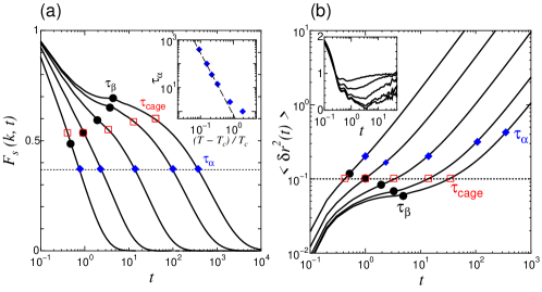
Figure 2: (a) Intermediate scattering function $F_{s}(k,t)$ with $k=2\pi$ and (b) Mean square displacement $\langle\delta r^{2}(t)\rangle$ at temperatures $T=0.772$, $0.473$, $0.352$, $0.306$, and $0.289$ from left to right for the model system described in Sec. 4. The time scales $\tau_{\beta}$, $\tau_{\rm Int}$, and $\tau_{\alpha}$ are indicated by circles, squares, and diamonds, respectively. These time scales are described in Sec. 4. The dotted line represents (a) $F_{s}(k,t)=1/e$ and (b) $\langle\delta r^{2}(t)\rangle=0.1$, respectively. Inset of (a): $\alpha$-relaxation time $\tau_{\alpha}$ as a function of the temperature $(T-T_{c})/T_{c}$ with $T_{c}=0.265$. The dashed line refers to power-law behavior as $\tau_{\alpha}\sim(T-T_{c})^{-\gamma}$ with $\gamma=2.6$. Inset of (b): $\mathrm{d}\ln\langle\delta r^{2}(t)\rangle/\mathrm{d}\ln t$ at temperatures $T=0.772$, $0.473$, $0.352$, $0.306$, and $0.289$ from top to bottom.

where $\sigma_{ab}=(\sigma_{a}+\sigma_{b})/2$ and $a,b\in\{1,2\}$. The interaction was truncated at $r=3\sigma_{1}$. The size and mass ratios were taken to be $\sigma_{1}/\sigma_{2}=1/1.2$ and $m_{1}/m_{2}=1/2$, respectively. The total number density was fixed at $\rho=(N_{1}+N_{2})/L^{3}=0.8\sigma_{1}^{-3}$ with the system length $L=29.24\sigma_{1}$ under periodic boundary conditions. In this study, the numerical results will be presented in terms of reduced units $\sigma_{1}$, $\epsilon_{0}/k_{B}$, and $\tau=\sqrt{m_{1}\sigma_{1}^{2}/\epsilon_{0}}$ for length, temperature, and time, respectively. The velocity Verlet algorithm was used with a time step of $0.005\tau$ in the microcanonical ensemble. The investigated thermodynamic states were $T\in[0.772,0.289]$. At each temperature, the self-part of the intermediate scattering function for the component $1$, $F_{s}(k,t)$, is calculated with the wave number $k_{\rm max}=2\pi/\sigma_{1}$, at which the static structure factor of component $1$ takes its first peak. The $\alpha$-relaxation time $\tau_{\alpha}$ is determined from the criterion $F_{s}(k_{\rm max},\tau_{\alpha})=e^{-1}$, as shown in Fig. 2(a). The “mode-coupling” transition temperature $T_{c}$ is evaluated from the power law behavior as $\tau_{\alpha}\sim(T-T_{c})^{-\gamma}$ with $T_{c}\simeq 0.265$ and $\gamma\simeq 2.6$. The relative temperature distance from $T_{c}$ is given as $\epsilon=(T-T_{c})/T_{c}\in[1.91,0.09]$. To determine the smaller time scale of the $\beta$-relaxation, we define the time $\tau_{\beta}$ at which the function $\mathrm{d}\ln\langle\delta r^{2}(t)\rangle/\mathrm{d}\ln t$ has the minimum value ²⁴. Here $\langle\delta r^{2}(t)\rangle$ is the mean square displacement for component $1$. Furthermore, we determine the intermediate time scale, that is referred to as $\tau_{\rm Int}$, between the two time scales $\tau_{\beta}$ and $\tau_{\alpha}$. This time scale $\tau_{\rm Int}$ is determined from the criterion as $\langle\delta r^{2}(\tau_{\rm Int})\rangle=0.1{\sigma_{1}}^{2}$. As observed in Fig. 2(b), after this time the tagged particle can escape from the cage composed of neighboring particles, particularly at lower temperatures. On the other hand, at high temperatures, $\tau_{\rm Int}$ is approximately equal to $\tau_{\beta}$. Figure 2(b) shows the time dependence of the MSD, where three time scales $\tau_{\beta}$, $\tau_{\rm Int}$, and $\tau_{\alpha}$ are shown at each temperature.

In the IMD, we have performed simulations in the linear response regime with $h=0.02$. After long time simulations comparable to the $\alpha$-relaxation time $\tau_{\alpha}$, the density field $\rho(\bm{r},t)$ reaches a stationary state following the profile of $\cos(\bm{q}\cdot\bm{r})$. Then, the correlation function Eq. (7) was calculated. We averaged the results over 30 independent simulation runs. The simulation time at lowest temperature is as long as $t=100,000$.

5 Results and Discussion

5.1 Four-point correlation function $S_{4}(q,t)$

We first summarize the numerical results by using the four-point correlation functions obtained from the EQMD simulations. We follow previously established work ^{12, 15, 17, 22}, with the four-point correlation function $S_{4}(q,t)$ defined as

$$S_{4}(q,t)=\frac{1}{N}\langle Q(\bm{q},t)Q(-\bm{q},t)\rangle,$$ (13)

$$Q(\bm{q},t)=\sum_{i=1}^{N}W_{i}(a,t)\exp[-i\bm{q}\cdot\bm{r}_{i}(0)],$$ (14)

with $q=|\bm{q}|$. Here $W_{i}(a,t)=\Theta(a-|\bm{r}_{i}(t)-\bm{r}_{i}(0)|)$ is the overlap function or Heaviside step function $\Theta(x)$. $W_{i}(a,t)$ selects the particle that moves farther than distance $a$ during the time interval $t$. We use $a=0.3\sigma_{1}$ in this study.

The behavior of $S_{4}(q,t)$ at small wave numbers is conventionally described by the Ornstein–Zernike (OZ) form as follows:

$$S_{4}(q,t)=\frac{\chi_{4}(t)}{1+(q\xi_{4}(t))^{\alpha}},$$ (15)

where $\xi_{4}(t)$ is the correlation length and $\chi_{4}(t)$ is the intensity at $q\to 0$. As mentioned previously, it is an intricate task to numerically obtain quantities such as the dynamical length scale from $S_{4}(q,t)$ in the $q\to 0$ limit. While our system size is smaller than optimal, we note that earlier work in the same system with $N_{1}+N_{2}=100,000$ has presented extracted lengths consistent with those we find here using the same method ³⁰. Furthermore, the procedure we use to extract the dynamical length scale $\xi_{4}(t)$, while not as rigorous is that used in Refs  27, 28, has shown consistency in extracted length values in the same system (compare the results of Ref.  22 to those of Ref.  26)

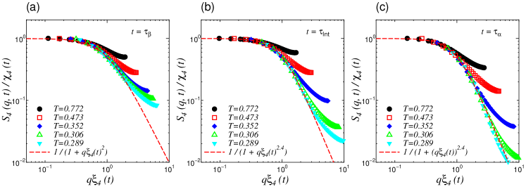
Figure 3: Scaled four-point correlation function $S_{4}(q,t)/\chi_{4}(t)$ as a function of $q\xi_{4}(t)$ at $T=0.772$, $0.473$, $0.352$, $0.306$, and $0.289$. The time interval $t$ is chosen as (a) $\tau_{\beta}$, (b) $\tau_{\rm Int}$, and (c) $\tau_{\alpha}$. The dashed line represents the Ornstein–Zernike form $1/(1+(q\xi_{4}(t))^{\alpha})$ with (a) $\alpha=2$, (b) $\alpha=2.4$, and (c) $\alpha=2.4$, respectively.

As shown in Fig. 3(a), the results at the small time scale $t=\tau_{\beta}$ are well described by Eq. (15) with $\alpha=2$, which is the typical the OZ behaviour ^{12, 16, 17}. In contrast, we find that for large time scales $t=\tau_{\rm Int}$ and $\tau_{\alpha}$, the slope of $S_{4}(q,t)$ becomes gradually sharper, which is more compatible with a power $S_{4}(q,\tau_{\alpha})\sim q^{-2.4}$ particularly at lower temperatures, as demonstrated in Figs. 3(b) and (c). Similar power law behavior at $\alpha$-relaxation time has been reported in the Kob–Andersen systems ²². We also note that the same exponent $\alpha=2.4$ has been reported in the binary soft-sphere mixture with a larger system size $N_{1}+N_{2}=100,000$ ³⁰. Thus, we choose $\alpha=2.4$ of Eq. (15) and determine $\xi_{4}(t)$ and $\chi_{4}(t)$ at two time scales $t=\tau_{\rm Int}$ and $\tau_{\alpha}$ for various temperatures.

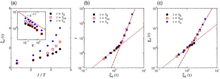
Figure 4: (a) Inverse temperature $1/T$ dependence of the length $\xi_{4}(t)$ at time scale $t=\{\tau_{\beta},\tau_{\rm Int},\tau_{\alpha}\}$. Inset: $\xi_{4}$ as a function of $\epsilon=(T-T_{c})/T_{c}$. The dotted line represents the power law slope of $\xi_{4}\sim\epsilon^{-0.5}$. (b) Relationship between the time scale $t=\{\tau_{\beta},\tau_{\rm Int},\tau_{\alpha}\}$ and length $\xi_{4}(t)$ for various temperatures. The dotted and dashed lines denotes the power law relationships of $t\sim{\xi_{4}(t)}^{z}$ with $z=5$ and $z=1.6$, respectively. (c) Relationship between the intensity $\chi_{4}(t)$ and length $\xi_{4}(t)$ at time scale $t=\{\tau_{\beta},\tau_{\rm Int},\tau_{\alpha}\}$ for various temperatures. The dotted and dashed lines denote the power law relationships of $\chi_{4}(t)\sim{\xi_{4}(t)}^{2-\eta}$ with $2-\eta=2.6$ and $2-\eta=1.2$, respectively.

The temperature dependence of the qualified length scale $\xi_{4}(t)$ at $t=\{\tau_{\beta},\tau_{\rm Int},\tau_{\alpha}\}$ is shown in Fig 4(a). It is demonstrated that $\xi_{4}(t)$ at each time scale $t$ grows with decreasing temperature. In particular, we observe the power law behavior $\xi_{4}(\tau_{\alpha})\sim\epsilon^{-\nu}$ with $\nu\approx 0.5$ at the time scale of $\tau_{\alpha}$. Note that IMCT instead predicts the exponent $\nu=0.25$ ³⁸. Thus, as found previously for a Kob–Andersen Lennard–Jones mixture, the IMCT results are not compatible with the growth of $\xi_{4}(\tau_{\alpha})$ ^{22, 26, 30}. In addition, we examine the scaling relationships between the time scale $t$ and length $\xi_{4}(t)$ and between the intensity $\chi_{4}(t)$ and $\xi_{4}(t)$, which are demonstrated in Figs. 4(b) and (c), respectively. The relationships are obtained as $\tau_{\alpha}\sim\xi_{4}(\tau_{\alpha})^{z}$ with $z\approx\gamma/\nu\approx 5$ and $\chi_{4}(\tau_{\alpha})\sim\xi_{4}(\tau_{\alpha})^{2-\eta}$ with $2-\eta\approx\alpha\approx 2.6$, which are similar to those found in other systems. We also find the relationships at the $\beta$-relaxation time regime with the smaller exponents, $z\approx 1.6$ and $2-\eta\approx 1.2$, as observed in Figs. 4(b) and (c). At the intermediate time scale of $\tau_{\rm Int}$, the cross-overs between two time scales, $\tau_{\beta}$ and $\tau_{\alpha}$, are observed in those relationships.

5.2 Three-point correlation function $\chi_{u}(k,q,t)$

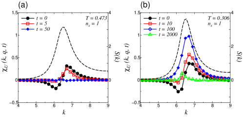
Figure 5: Wave number $k$ dependence of the three-point correlation function $\chi_{U}(k,q,t)$ at (a) $T=0.473$ and (b) $T=0.306$ at time interval $t$ using the left axis. $n_{x}=1$ corresponds to the smallest wave number $q_{\rm min}=2\pi/L\simeq 0.215$. For comparison, the static structure factor $S(k)$ at each temperature is plotted as a dashed line using the right axis.

Here we present the numerical results of the three-point correlation functions $\chi_{U}(k,q,t)$ obtained from the IMD simulations, as outlined in Sec. 2. First, we show the wave number $k=|\bm{k}|$ dependence of $\chi_{U}(k,q,t)$ for various time intervals $t$ in Fig. 5. It is observed that at initial time $t=0$, the profile of $\chi_{U}(k,q,t)$ is proportional to $\mathrm{d}S(k)/\mathrm{d}k$. This property is reported in the mode-coupling calculation performed in Ref.  39. At high temperature ($T=0.473$), the peak of $\chi_{U}(k,q,t)$ monotonically decreases as the time $t$ proceeds. In contrast, at the supercooled state ($T=0.306$), $\chi_{U}(k,q,t)$ develops a peak at the wave number where $S(k)$ has its first peak, around $k\simeq 6.6$ when the time interval approaches around the $\alpha$-relaxation, $\tau_{\alpha}(\simeq 100)$. For larger times of $t\to\infty$, $\chi_{U}(k,q,t)$ tends to decrease and finally becomes zero at any wave number $k$.

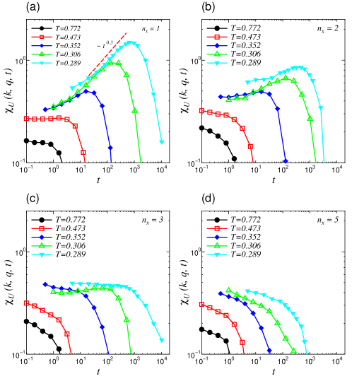
Figure 6: Time evolution of the three-point correlation function $\chi_{U}(k,q,t)$ at $T=0.772$, $0.473$, $0.352$, $0.306$, and $0.289$. Wave number $q$ is chosen as $q=2\pi n_{x}/L$ with (a) $n_{x}=1$, (b) $n_{x}=2$, (c) $n_{x}=3$, and (d) $n_{x}=5$. T wave number $k$ is averaged over the range $k\in[6.5,6.8]$.

To observe how the three-point correlation function $\chi_{U}(k,q,t)$ grows with time $t$, the time evolutions of $\chi_{U}(k,q,t)$ at various temperatures are shown in Fig. 6. Here the wave number $q=2\pi n_{x}/L$ of the external field is changed as (a) $n_{x}=1$, (b) $n_{x}=2$, (c) $n_{x}=3$, and (d) $n_{x}=5$. We averaged $\chi_{U}(\bm{k},\bm{q},t)$ over wave vectors $\bm{k}$ in the range of $k\in[6.5,6.8]$ to suppress statistical errors. It is observed that the intensity of $\chi_{U}(k,q,t)$ with the smallest wave number $n_{x}=1$ has its maximum value at the $\alpha$-relaxation time $\tau_{\alpha}$. This basic feature of $\chi_{U}(k,q,t)$ is also demonstrated in both the four-point susceptibilities $\chi_{4}(t)=\lim_{q\to 0}S_{4}(q,t)$ and as predicted by IMCT. However, the time dependence of $\chi_{U}$ appears to grow as $t^{0.3}$ even at low temperature, which is milder than that the growth $t^{0.7}$ we found for $\chi_{4}(t)$. In addition, IMCT predicts $\chi_{U}\sim t^{b}$ with $b\approx 0.6$ in the late $\beta$ regime and $t^{a}$ with $a\approx 0.3$ in the early $\beta$ regime. The reason for this discrepancy between $\chi_{4}$ and IMCT is unclear. As already discussed the behavior of $\chi_{4}$ obtained as $q\rightarrow 0$ limit of $S_{4}$ is quite intricate because, roughly speaking, it is expected to be given by two terms: one proportional to $\chi_{U}$ and another proportional to its square. The latter becoming important very close to $T_{MCT}$ but negligible far from it ^{22, 23}. Thus obtaining reliable values of critical exponents from $\chi_{4}$ and $S_{4}$ is quite difficult. Another possibility is that the investigated temperatures herein are still quite limited. As shown in Fig. 2(a), even for the lowest temperature, the two-step relaxation of the intermediate scattering function is not well developed, making it difficult to distinguish between the early and late $\beta$-relaxation regime. Such limitations are imposed by the numerical difficulty in obtaining well-averaged values of $\chi_{U}(k,q,t)$ from IMD.

Next, we examine the wave number $q$ dependence of the three-point correlation function $\chi_{U}(k,q,t)$, which should be compared with the four-point correlation function shown in Fig. 3. As shown in Fig. 6 the pronounced peak of $\chi_{U}$ rapidly decreases as the wave number $q=2\pi n_{x}/L$ is increased, particularly at lower temperature. To describe $\chi_{U}(k,q,t)$ and extract the length scale, let us consider a generalized OZ form including a $q^{-4}$ term as

$$\chi_{U}(k,q,t)=\frac{\chi_{U}(t)}{1+(q\xi_{U}(t))^{2}+A(q\xi_{U}(t))^{4}}.$$ (16)

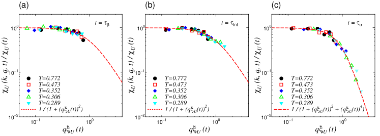
Figure 7: Scaled three-point correlation function $\chi_{U}(k,q,t)/\chi_{U}(t)$ as a function of $q\xi_{U}(t)$ at $T=0.772$, $0.473$, $0.352$, $0.306$, and $0.289$. The time interval $t$ is chosen as (a) $\tau_{\beta}$, (b) $\tau_{\rm Int}$ (b), and (c) $\tau_{\alpha}$. The dashed line represents the generalized OZ form $1/(1+(q\xi_{U}(t))^{2}+A((q\xi_{U}(t))^{4})$ with $A=0$ for (a) $t=\tau_{\beta}$ and (b) $\tau_{\rm Int}$, and (c) with $A=1$ for $t=\tau_{\alpha}$, respectively.

Note that this $q^{-4}$ scaling is predicted by IMCT at the $\alpha$-relaxation time. In the same way as Eq. (15), $\xi_{U}(t)$ and $\chi_{U}(t)$ express the length scale and intensity at $q\to 0$, respectively. Figure 7 shows the scaled $\chi_{U}(k,q,t)/\chi_{U}(t)$ at various time scales $t=\tau_{\beta}$, $\tau_{\rm Int}$, and $\tau_{\alpha}$. First, as observed in Figs. 7(a) and (b), $\chi_{U}(k,q,t)$ is well described by Eq. (16) with $A=0$ at the time scales, $t=\tau_{\beta}$ and $\tau_{\rm Int}$, corresponding to the usual OZ form. In contrast, at the time scale $t=\tau_{\alpha}$, the wave number $q$ dependence of $\chi_{U}(k,q,t)$ becomes steeper than in $\chi_{U}(k,q,t)$ at smaller times $t=\tau_{\beta}$ and $\tau_{\rm Int}$, as demonstrated in Fig. 7(c). This behavior can be described by the expression in Eq. (16) including the fourth order correction with $A=1$. The observed cross-over of the function form $\chi_{U}$ from the vicinity of $\beta$-relaxation to $\alpha$-relaxation is apparently different from the behavior of the four-point correlations $S_{4}(q,t)$ observed in Fig. 3; however, alternatively, it is in accordance with the non-trivial prediction of IMCT ³⁸. Here we note that within IMCT the $q^{-4}$ scaling is not well developed in the supercooled state ($\epsilon\simeq 0.1$) but instead becomes clear much closer to $T_{MCT}$ (e.g. $\epsilon\leq 10^{-3}$) ³⁹. In this sense this distinction may well be an indicator of alteration of the mean field behavior predicted by IMCT.

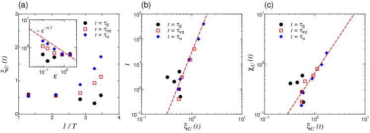
Figure 8: (a) Temperature dependence of $\xi_{4}(\tau_{\alpha})$ and $\xi_{U}(\tau_{\alpha})$. Inset: $\xi_{U}(\tau_{\alpha})$ as a function of $\epsilon=(T-T_{c})/T_{c}$. The dashed line is the power law slope of $\epsilon^{-0.5}$. (b) Relationship between the time scale $t=\{\tau_{\beta},\tau_{\rm Int},\tau_{\alpha}\}$ and length scale $\xi_{U}(t)$ for various temperatures. The dotted line is the power law relation, $t\sim{\xi_{U}}^{5}$. (c) Relationship between the intensity $\chi_{U}(t)$ and length $\xi_{U}(t)$ on the time scale $t=\{\tau_{\beta},\tau_{\rm Int},\tau_{\alpha}\}$ for various temperatures. The dashed line is the power law relationship, $\chi_{U}\sim{\xi_{U}}^{1.5}$.

The determined length scale $\xi_{U}(t)$ is shown as a function of temperature $T$ in Fig. 8(a) at times, $t={\tau_{\beta}}$, $\tau_{\rm Int}$, and $\tau_{\alpha}$. Similar to the temperature dependence of the length scale $\xi_{4}$ extracted from the four-point correlator, the length scale $\xi_{U}(\tau_{\alpha})$ increases with decreasing temperature. Although the evaluated value $\xi_{U}(\tau_{\alpha})$ is smaller than $\xi_{4}(\tau_{\alpha})$, $\xi_{U}(\tau_{\alpha})$ can be approximated by $\xi_{U}(\tau_{\alpha})\sim\epsilon^{-\nu}$ with $\nu\approx 0.5$, which is same as the $\xi_{4}(\tau_{\alpha})$ (see Fig. 4(a)). Since absolute length scales are not obtained via the scaling analysis performed here, the agreement in scaling between $\xi_{U}(\tau_{\alpha})$ and $\xi_{4}(\tau_{\alpha})$ should be taken as preliminary confirmation of the generic prediction from the analysis of Ref.  22 that $\xi_{U}\sim\xi_{4}$. Furthermore, the relationship $\tau_{\alpha}\sim\xi_{U}(\tau_{\alpha})^{z}$ with $z\approx 5$ is observed in Fig. 8(b). This exponent is close to the value of $\xi_{4}(\tau_{\alpha})$, as obtained in Fig. 4(b). We also obtain the relationship $\chi_{U}(\tau_{\alpha})\sim\xi_{U}(\tau_{\alpha})^{2-\eta_{\alpha}}$ with $2-\eta_{\alpha}\approx 1.5$ in Fig. 8(c). This exponent is rather smaller than that of $\xi_{4}(\tau_{\alpha})$ obtained in Fig. 4(c). A disagreement with the IMCT prediction $2-\eta_{\alpha}=4$ is also observed. In addition, as shown in Fig. 8(a), the length scale $\xi_{U}(\tau_{\beta})$ at $\tau_{\beta}$ is not available because of the large numerical fluctuations. Here it can be considered that the minimum wave number of the present system $q_{\rm min}=2\pi/L\simeq 0.215$ is still too large to reduce those numerical errors. As mentioned above, it is an important future goal to seek lower temperature data approaching the mode-coupling transition temperature. In particular, further analysis for larger systems and lower temperatures is necessary to improve the signal-to-noise ratio of the response function and acquire more insight into the behavior of $\chi_{U}$.

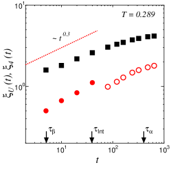
Figure 9: Time dependence of the length scales $\xi_{4}(t)$ (squares) and $\xi_{U}(t)$ (circles) at the lowest temperature $T=0.289$. The time values $\tau_{\alpha}$, $\tau_{\rm Int}$, and $\tau_{\beta}$ are indicated by arrows. Note that for the length scale $\xi_{U}(t)$, the closed and open symbols denote $\xi_{U}(t)$ evaluated by the generalized OZ form Eq. (16) with $A=0$ and $A=1$, respectively. This switch is responsible for the small gap of $\xi_{U}$ around $\tau_{\rm Int}$.

Finally, the physical implementation of the time-scale dependence of the function form $\chi_{U}$ is worthy of mention. As discussed in Ref.  38, this cross-over of the scaling function might be relevant to the geometrical change of dynamically correlated motions. Namely, IMCT predicts that the dynamic length scale $\xi_{U}(t)$ increases at the early $\beta$ regime and then saturates to a constant value at the late $\beta$ regime. This suggests that while keeping a constant spatial extent, the geometrical structure of the dynamic correlations significantly fatten between $\tau_{\beta}$ and $\tau_{\alpha}$. Recent MD simulations reveal that the mobile particle motions form string-like structures in the $\beta$-relaxation regime ⁴⁴, whereas a more compact structure is observed at the slower time scale of $\tau_{\alpha}$ ⁴⁵. In Fig. 9, we show the time evolution of the length scales $\xi_{4}(t)$ and $\xi_{U}(t)$ at the lowest temperature $T=0.289$. Although it is difficult to distinguish between early and late $\beta$ regimes in the present simulation, we observe that both length scales tend to increase from $\tau_{\beta}$ and saturate around the time exceeding $\tau_{\rm Int}$ in a similar manner. After the time scale $\tau_{\rm Int}$ a better description of $\chi_{U}$ is obtained with the fourth-order corrections in the generalized OZ form, Eq. (16), as shown in Fig. 7(c).

6 Summary and Conclusions

In Refs.  22, 23 it was argued on general grounds, beyond the particularities of mean-field predictions that originate from theories such as IMCT, that the function $\chi_{U}(\bm{k},\bm{q},t)$, which is the response of the two-point correlation function with respect to an inhomogeneous external field, offers particular advantages over the more conventional $S_{4}(q,t)$. For these reasons we have investigated the function $\chi_{U}(\bm{k},\bm{q},t)$ to quantitatively characterize the length scale of dynamic heterogeneity via IMD simulations. As predicted by IMCT, we did find that $\xi_{U}$ probe dynamic correlations and that the associated dynamic correlation length scales similarly to the one extracted from $S_{4}$. Therefore $\xi_{U}$ provides a viable alternative to $\chi_{4}$ and $S_{4}$: its advantages are an enhanced possibility for experimental extraction in colloidal systems, as well as a simpler ensemble and temperature dependence. Thus extracting critical properties of $\chi_{4}$ is quite delicate.

We also compared the critical behavior of $\chi_{U}$ obtained in simulations to IMCT results. Although some predictions are verified, as the cross-over from the $q^{-2}$ decay to the sharper $q^{-4}$ decay when the time scale changes from $\tau_{\beta}$ to $\tau_{\alpha}$, others are not. For example the values of $\nu$ and $z_{\alpha},z_{\beta}$ are off by a substantial amount. Moreover, there is a discrepancy between the value of $\eta_{\alpha}$ obtained from the $q^{-4}$ decay, which is in agreement with IMCT, and the one obtained by the relation $\chi_{4}(\tau_{\alpha})\propto\xi_{U}(\tau_{\alpha})^{2-\eta_{\alpha}}$. This difference could either indicate a breakdown of usual scaling laws or, more simply, that the systems is not close enough to the critical point and, hence, there is a substantial error in the values of the exponents. We have indications that the latter option is the most likely one. Further analysis is necessary to assess the behavior of $\chi_{U}(\bm{k},\bm{q},t)$ more critically in a much larger and varied systems and at a lower temperatures.

Finally, it is important to recall that the IMCT exponents are mean-field ones and that the upper critical dimension for the MCT transition is $d_{u}=8$ ^{46, 47}. In fact, as previously mentioned, in three dimensions non-mean field fluctuations such thermally activated hopping motion occurs. In consequence, the fact that IMCT works qualitatively but not quantitatively is actually a promising evidence that dynamic correlations close to $T_{MCT}$ can be indeed described in terms of a dynamical critical MCT phenomenon but that in order to reach quantitative agreement a theory of critical fluctuations valid below $d_{u}$ has to be constructed. Progress in this direction have been recently obtained in Refs. 47, 48.

We thank J.-P. Bouchaud for discussions and collaboration on the topics addressed in this work, in particular IMCT. K.K. was supported by Grants-in-Aid for Scientific Research: Young Scientists (A) No. 23684037 from Japan Society for the Promotion of Science (JSPS). D.R.R. was supported by NSF CHE-1213247. G.B. was supported by the ERC grant NPRGGLASS. K.K. acknowledges Yamada Science Foundation for supporting his stay at Columbia University in 2011. The computations were performed at Research Center for Computational Science, Okazaki Research Facilities, National Institutes of Natural Sciences, Japan.

Figure 1: Schematic illustration of the calculation procedure for the three-point correlation function $\chi_{U}(\bm{k},\bm{q},t)$ via the hybrid IMD and EQMD simulations. The IMD line represents the ramping profile for the external force of Eq. (6).

References

- Wolynes and Lubchenko 2012 Wolynes, P. G.; Lubchenko, V. Structural Glasses and Supercooled Liquids; John Wiley & Sons, USA, 2012
- Ediger et al. 1996 Ediger, M. D.; Angell, C. A.; Nagel, S. R. Supercooled Liquids and Glasses. J. Phys. Chem. 1996, 100, 13200–13212
- Debenedetti and Stillinger 2001 Debenedetti, P. G.; Stillinger, F. H. Supercooled liquids and the glass transition. Nature 2001, 410, 259–267
- Lubchenko and Wolynes 2007 Lubchenko, V.; Wolynes, P. G. Theory of Structural Glasses and Supercooled Liquids. Annu. Rev. Phys. Chem. 2007, 58, 235–266
- Cavagna 2009 Cavagna, A. Supercooled liquids for pedestrians. Phys. Rep. 2009, 476, 51–124
- Berthier and Biroli 2011 Berthier, L.; Biroli, G. Theoretical perspective on the glass transition and amorphous materials. Rev. Mod. Phys. 2011, 83, 587–645
- Berthier et al. 2011 Berthier, L., Biroli, G., Bouchaud, J.-P., Cipelletti, L., van Saarloos, W., Eds. Dynamical Heterogeneities in Glasses, Colloids, and Granular Media; Oxford University Press: USA, 2011
- Ediger 2000 Ediger, M. D. Spatially heterogeneous dynamics in supercooled liquids. Annu. Rev. Phys. Chem. 2000, 51, 99–128
- Hurley and Harrowell 1995 Hurley, M. M.; Harrowell, P. Kinetic structure of a two-dimensional liquid. Phys. Rev. E 1995, 52, 1694–1698
- Kob et al. 1997 Kob, W.; Donati, C.; Plimpton, S. J.; Poole, P. H.; Glotzer, S. C. Dynamical Heterogeneities in a Supercooled Lennard-Jones Liquid. Phys. Rev. Lett. 1997, 79, 2827
- Yamamoto and Onuki 1997 Yamamoto, R.; Onuki, A. Kinetic Heterogeneities in a Highly Supercooled Liquid. J. Phys. Soc. Jpn. 1997, 66, 2545–2548
- Yamamoto and Onuki 1998 Yamamoto, R.; Onuki, A. Dynamics of highly supercooled liquids: Heterogeneity, rheology, and diffusion. Phys. Rev. E 1998, 58, 3515–3529
- Franz and Parisi 2000 Franz, S.; Parisi, G. On non-linear susceptibility in supercooled liquids. J. Phys.: Condens. Matter 2000, 12, 6335–6342
- Donati et al. 2002 Donati, C.; Franz, S.; Glotzer, S. C.; Parisi, G. Theory of non-linear susceptibility and correlation length in glasses and liquids. J. Non-Cryst. Solids 2002, 307-310, 215–224
- Lačević et al. 2002 Lačević, N.; Starr, F.; Schrøder, T.; Novikov, V.; Glotzer, S. Growing correlation length on cooling below the onset of caging in a simulated glass-forming liquid. Phys. Rev. E 2002, 66, 030101
- Lačević et al. 2003 Lačević, N.; Starr, F. W.; Schrøder, T. B.; Glotzer, S. C. Spatially heterogeneous dynamics investigated via a time-dependent four-point density correlation function. J. Chem. Phys. 2003, 119, 7372–7387
- Berthier 2004 Berthier, L. Time and length scales in supercooled liquids. Phys. Rev. E 2004, 69, 020201(R)
- Whitelam et al. 2004 Whitelam, S.; Berthier, L.; Garrahan, J. P. Dynamic Criticality in Glass-Forming Liquids. Phys. Rev. Lett. 2004, 92, 185705
- Toninelli et al. 2005 Toninelli, C.; Wyart, M.; Berthier, L.; Biroli, G.; Bouchaud, J. P. Dynamical susceptibility of glass formers: Contrasting the predictions of theoretical scenarios. Phys. Rev. E 2005, 71, 041505
- Chandler et al. 2006 Chandler, D.; Garrahan, J. P.; Jack, R. L.; Maibaum, L.; Pan, A. C. Lengthscale dependence of dynamic four-point susceptibilities in glass formers. Phys. Rev. E 2006, 74, 051501
- Szamel and Flenner 2006 Szamel, G.; Flenner, E. Four-point susceptibility of a glass-forming binary mixture: Brownian dynamics. Phys. Rev. E 2006, 74, 021507
- Berthier et al. 2007 Berthier, L. et al. Spontaneous and induced dynamic fluctuations in glass formers. I. General results and dependence on ensemble and dynamics. J. Chem. Phys. 2007, 126, 184503
- Berthier et al. 2007 Berthier, L. et al. Spontaneous and induced dynamic correlations in glass formers. II. Model calculations and comparison to numerical simulations. J. Chem. Phys. 2007, 126, 184504
- Stein and Andersen 2008 Stein, R. S. L.; Andersen, H. C. Scaling Analysis of Dynamic Heterogeneity in a Supercooled Lennard-Jones Liquid. Phys. Rev. Lett. 2008, 101, 267802
- Karmakar et al. 2009 Karmakar, S.; Dasgupta, C.; Sastry, S. Growing length and time scales in glass-forming liquids. Proc. Natl. Acad. Sci. U.S.A. 2009, 106, 3675–3679
- Karmakar et al. 2010 Karmakar, S.; Dasgupta, C.; Sastry, S. Analysis of Dynamic Heterogeneity in a Glass Former from the Spatial Correlations of Mobility. Phys. Rev. Lett. 2010, 105, 015701
- Flenner and Szamel 2010 Flenner, E.; Szamel, G. Dynamic Heterogeneity in a Glass Forming Fluid: Susceptibility, Structure Factor, and Correlation Length. Phys. Rev. Lett. 2010, 105, 217801
- Flenner et al. 2011 Flenner, E.; Zhang, M.; Szamel, G. Analysis of a growing dynamic length scale in a glass-forming binary hard-sphere mixture. Phys. Rev. E 2011, 83, 051501
- Mizuno and Yamamoto 2011 Mizuno, H.; Yamamoto, R. Dynamical heterogeneity in a highly supercooled liquid: Consistent calculations of correlation length, intensity, and lifetime. Phys. Rev. E 2011, 84, 011506
- Kim and Saito 2013 Kim, K.; Saito, S. Multiple length and time scales of dynamic heterogeneities in model glass-forming liquids: A systematic analysis of multi-point and multi-time correlations. J. Chem. Phys. 2013, 138, 12A506
- Berthier et al. 2005 Berthier, L. et al. Direct Experimental Evidence of a Growing Length Scale Accompanying the Glass Transition. Science 2005, 310, 1797–1800
- Dalle-Ferrier et al. 2007 Dalle-Ferrier, C. et al. Spatial correlations in the dynamics of glassforming liquids: Experimental determination of their temperature dependence. Phys. Rev. E 2007, 76, 041510
- Brambilla et al. 2009 Brambilla, G. et al. Probing the Equilibrium Dynamics of Colloidal Hard Spheres above the Mode-Coupling Glass Transition. Phys. Rev. Lett. 2009, 102, 085703
- Bouchaud and Biroli 2005 Bouchaud, J. P.; Biroli, G. Nonlinear susceptibility in glassy systems: A probe for cooperative dynamical length scales. Phys. Rev. B 2005, 72, 064204
- Tarzia et al. 2010 Tarzia, M.; Biroli, G.; Lefèvre, A.; Bouchaud, J. P. Anomalous nonlinear response of glassy liquids: General arguments and a mode-coupling approach. J. Chem. Phys. 2010, 132, 054501
- Crauste-Thibierge et al. 2010 Crauste-Thibierge, C. et al. Evidence of Growing Spatial Correlations at the Glass Transition from Nonlinear Response Experiments. Phys. Rev. Lett. 2010, 104, 165703
- Diezemann 2012 Diezemann, G. Nonlinear response theory for Markov processes: Simple models for glassy relaxation. Phys. Rev. E 2012, 85, 051502
- Biroli et al. 2006 Biroli, G.; Bouchaud, J. P.; Miyazaki, K.; Reichman, D. R. Inhomogeneous Mode-Coupling Theory and Growing Dynamic Length in Supercooled Liquids. Phys. Rev. Lett. 2006, 97, 195701
- Szamel and Flenner 2010 Szamel, G.; Flenner, E. Diverging length scale of the inhomogeneous mode-coupling theory: A numerical investigation. Phys. Rev. E 2010, 81, 031507
- Curtis et al. 2002 Curtis, J. E.; Koss, B. A.; Grier, D. G. Dynamic holographic optical tweezers. Optics Commun. 2002, 207, 169–175
- Ciccotti et al. 1979 Ciccotti, G.; Jacucci, G.; McDonald, I. R. ”Thought-experiments” by molecular dynamics. J. Stat. Phys. 1979, 21, 1–22
- Bernu et al. 1985 Bernu, B.; Hiwatari, Y.; Hansen, J. P. A molecular dynamics study of the glass transition in binary mixtures of soft spheres. J. Phys. C 1985, 18, L371–L376
- Bernu et al. 1987 Bernu, B.; Hansen, J. P.; Hiwatari, Y.; Pastore, G. Soft-sphere model for the glass transition in binary alloys: Pair structure and self-diffusion. Phys. Rev. A 1987, 36, 4891
- Donati et al. 1998 Donati, C. et al. Stringlike Cooperative Motion in a Supercooled Liquid. Phys. Rev. Lett. 1998, 80, 2338–2341
- Appignanesi et al. 2006 Appignanesi, G. A.; Rodríguez Fris, J. A.; Montani, R. A.; Kob, W. Democratic Particle Motion for Metabasin Transitions in Simple Glass Formers. Phys. Rev. Lett. 2006, 96, 057801
- Biroli and Bouchaud 2007 Biroli, G.; Bouchaud, J.-P. Critical fluctuations and breakdown of the Stokes–Einstein relation in the mode-coupling theory of glasses. J. Phys.: Condens. Matter 2007, 19, 205101
- Franz et al. 2011 Franz, S.; Parisi, G.; Ricci-Tersenghi, F.; Rizzo, T. Field theory of fluctuations in glasses. Eur. Phys. J. E 2011, 34, 102
- Franz et al. 2010 Franz, S.; Parisi, G.; Ricci-Tersenghi, F.; Rizzo, T. Properties of the perturbative expansion around the mode-coupling dynamical transition in glasses. 2010, arXiv:1001.1746. arXiv.org e-Print archive. http://arxiv.org/abs/1001.1746 (accessed Jun 2010).