Testing assumptions and predictions of star formation theories

Abstract

We present numerical simulations of isothermal, magnetohydrodynamic (MHD), supersonic turbulence, designed to test various hypotheses frequently assumed in star formation (SF) theories. This study complements our previous one in the non-magnetic (HD) case. We consider three simulations, each with different values of its physical size, rms sonic Mach number ${\cal M}_{\rm s}$, and Jeans parameter $J$, but so that all three have the same value of the virial parameter and conform with Larson’s scaling relations. As in the non-magnetic case, we find that (1) no structures that are both subsonic and super-Jeans are produced; (2) that the fraction of small-scale super-Jeans structures increases when self-gravity is turned on, and the production of very dense cores by turbulence alone is very low. This implies that self-gravity is involved not only in the collapse of Jeans-unstable cores, but also in their formation. (3) We also find that denser regions tend to have a stronger velocity convergence, implying a net inwards flow towards the regions’ centres. Contrary to the non-magnetic case, we find that the magnetic simulation with lowest values of ${\cal M}_{\rm s}$ and $J$ (respectively, 5 and 2) does not produce any collapsing regions for over three simulation free-fall times, in spite of being both Jeans-unstable and magnetically supercritical. We attribute this result to the combined thermal and magnetic support. Next, we compare the results of our HD and MHD simulations with the predictions from the recent SF theories by Krumholz & McKee, Padoan & Nordlund, and Hennebelle & Chabrier, using expressions recently provided by Federrath & Klessen, which extend those theories to the magnetic case. In both the HD and MHD cases, we find that the theoretical predictions tend to be larger than the ${\rm SFE}_{\rm ff}$ measured in the simulations. In the MHD case, none of the theories captures the suppression of collapse at low values of $J_{\rm eff}$ by the additional support from the magnetic field. We conclude that randomly driven isothermal turbulence may not correctly represent the flow within actual clouds, and that theories that assume this regime may be missing a fundamental aspect of the flow. Finally, we suggest that a more realistic regime may be that of hierarchical gravitational collapse.

1 Introduction

Theories of star formation (SF) necessarily rely on assumptions about the structure of the molecular clouds (MCs) where the stars form. One of the most common of such assumptions is that the observed supersonic linewidths observed within MCs constitute supersonic turbulence (Zuckerman & Evans, 1974), and that this turbulence causes a net pressure that provides support against the clouds’ self-gravity, maintaining them in approximate virial equilibrium (e.g., Larson, 1981; Myers & Goodman, 1988; Blitz, 1993). The notion of turbulent pressure as an agent of support against self-gravity was first introduced by Chandrasekhar (1951) and later the scale-dependence of the turbulent support was also considered (e.g., Bonazzola et al., 1987; Vázquez-Semadeni & Gazol, 1995).

It is important to note that, in order for the non-thermal motions to be able to provide support against self-gravity, the turbulent velocity field must be essentially random. This property is actually extremely difficult to measure observationally, because one normally has information about only one component of the vector velocity field (the one along the line of sight), and moreover one does not have information about the spatial structure of that component along the line of sight. Thus, most measurements of the velocity structure in MCs refer to the magnitude of the velocity, which in turn is most commonly interpreted in terms of the non-thermal kinetic energy in the clouds, and its relative importance in the clouds’ virial balance, in particular in relation to the clouds’ gravitational energy (e.g., Mac Low & Klessen, 2004; McKee & Ostriker, 2007, and references therein). Statistical quantities, such as the kinetic energy spectrum in MCs (see, e.g., the review by Elmegreen & Scalo, 2004), give the distribution of the kinetic energy over the range of size scales present in the turbulent motions. However, this distribution is still obtained by averaging over the cloud’s volume, so no spatial information on the velocity field structure is provided by it.

Studies of the radial velocity gradient (e.g. Goldsmith & Arquilla, 1985; Goodman et al., 1993; Phillips, 1999; Caselli et al., 2002; Rosolowsky, 2007; Imara & Blitz, 2011; Imara et al., 2011; Li et al., 2012) provide a crude approximation to the spatial structure of the radial component of the velocity field across MCs. It must be noted that such gradients are most often interpreted as rotation, although in principle they might equally be interpreted as shear, expansion, or contraction. In fact, Brunt (2003) has pointed out that a principal component analysis of the clouds is inconsistent with that expected for uniform rotation, and instead interprets the inferred principal components of the velocity dispersion as large-scale chaotic turbulence (see also Brunt et al., 2009). Moreover, the possibility that the clouds are undergoing global contraction has been advocated by various recent studies (Vázquez-Semadeni et al., 2007, 2009; Heitsch & Hartmann, 2008; Ballesteros-Paredes et al., 2011a, b), in which case the gradients might be interpreted as the signature of this contraction. Thus, determination of the velocity field’s topology in MCs is a very important challenge for our understanding of their structure.

Another universal notion concerning SF is that, in MCs and their substructure, there exists a linewidth–size relation of the form (Larson, 1981)

$$\delta v_{\ell}\propto\ell^{\kappa},$$ (1)

and it is widely believed that such scaling relation originates as a consequence of the existence of a turbulent cascade, which produces a kinetic energy spectrum of the form $E(k)\propto k^{-n}$. Indeed, this form of the energy spectrum implies that the typical velocity difference across scales $\ell\sim 1/k$ is $\delta v_{\ell}\propto\ell^{(n-1)/2}$ (see, e.g., Vázquez-Semadeni et al., 2000). Thus, a spectral slope $n=5/3$ directly implies $\delta v_{\ell}\propto\ell^{1/3}$, close to the value $\kappa\approx 0.38$ initially observed by Larson (1981), while $n=2$ implies $\delta v_{\ell}\propto\ell^{1/2}$, as determined by most later studies (see, e.g., the review by Blitz, 1993, and references therein).

Larson (1981) also advanced a scaling relation between mean density and size, of the form

$$\langle\rho\rangle\propto\ell^{\lambda},$$ (2)

with $\lambda\sim-1$. Relations (1) and (2) are almost universally thought to be a manifestation of near virial equilibrium in the clouds, as originally proposed by Larson (1981) himself. However, the density–size relation has been questioned by a number of authors (e.g., Kegel, 1989; Scalo, 1990), in particular as it may be the result of an observational selection effect. Moreover, Ballesteros-Paredes et al. (2011a) have recently pointed out that the linewidth–size relation is in general not universally verified, and that it might also be a consequence of the same selection effects. Indeed, high-mass star-forming clumps typically exhibit larger linewidths for their size than those implied by the Larson (1981) relation (e.g., Caselli & Myers, 1995; Plume et al., 1997; Shirley et al., 2003; Gibson et al., 2009; Wu et al., 2010). Yet, Ballesteros-Paredes et al. (2011a) showed that, when the massive cores have mass determinations independent from virial estimates, it is found that their linewidth, size, and column density follow the general relation found by Heyer et al. (2009), namely

$$\delta v_{\ell}\propto\Sigma^{1/2}\ell^{1/2}.$$ (3)

The latter authors interpreted this scaling as evidence of virial equilibrium in clouds without constant column density, although Ballesteros-Paredes et al. (2011a) noted that this may just as well be interpreted as evidence of free-fall in the clouds and their substructures.

Within the context of the linewidth–size relation, equation (1), it is well known that such a relation implies that at some particular scale, termed the ‘sonic scale’ ($\lambda_{\rm s}$), the turbulent velocity dispersion is equal, on average, to the sound speed in the medium. Thus, a number of authors (e.g., Padoan, 1995; Vázquez-Semadeni et al., 2003; Krumholz & McKee, 2005; Federrath et al., 2010) have assumed that stars form in cores that have sizes equal to or smaller than the sonic scale, if they contain more than one thermal Jeans mass, since in these cores the main support is thermal. In principle, such cores can proceed to collapse without significant turbulent support nor fragmentation. Clumps larger than this scale are assumed to be globally supported against their self-gravity by turbulence, since they exhibit scaling relations like relation (3), and thus are interpreted as being near virial equilibrium. Nevertheless, within the clumps, the turbulence is assumed to induce local compressions that constitute smaller scale clumps and cores. However, if MCs are in a global state of gravitational collapse, as proposed by Vázquez-Semadeni et al. (2007, 2009), Heitsch & Hartmann (2008) and Ballesteros-Paredes et al. (2011a), then the observed linewidths may not reflect supporting turbulent motions, but rather the infall velocities themselves. In this case, the notion that the structures that collapse are the subsonic, super-Jeans cores may not apply.

In a previous paper (Vázquez-Semadeni et al., 2008, hereafter Paper I), we presented a numerical study designed to test the hypotheses mentioned above, using simulations of supersonic, isothermal, hydrodynamic driven turbulence. We considered three simulations with different physical box sizes, rms Mach numbers (${\cal M}_{\rm s}$), and Jeans numbers ($J=L/L_{\rm J}$, with $L$ the numerical box size and $L_{\rm J}$ the Jeans length), but such that the ratio ${\cal M}_{\rm s}/L_{\rm J}$ remained constant, thus assuring that the boxes followed Larson-type scaling relations (Larson, 1981). We found, among other results, that (a) there appeared to exist a negative correlation between the mean density and the mean velocity divergence of isolated subregions in the flow, suggesting that the velocity field is not completely random in overdense regions, but is characterized by a net convergence (negative divergence) of the velocity. The fact that the flow within the clumps has a net negative divergence instead of being fully random implies that not all of the flow’s kinetic energy is available for support against the self-gravity of the clump. (b) Clumps or subboxes of the numerical box with subsonic velocity tended to be Jeans stable, although significant gravitational collapse did occur in the simulations. This suggested that the main collapsing structures are large-scale, supersonic clumps, rather than small-scale, subsonic ones. (c) The SF efficiency per free-fall time of the various simulations, ${\rm SFE}_{\rm ff}$, scaled with ${\cal M}_{\rm s}$ roughly in agreement with the theoretical prediction by Krumholz & McKee (2005, hereafter KM05), within the (relatively large) uncertainties.

Since the publication of Paper I, two new theories have appeared (Hennebelle & Chabrier, 2011; Padoan & Nordlund, 2011), in addition to that by KM05, which attempt to describe the dependence of the star formation rate (SFR) on the main physical parameters of the clouds, namely the ratio of kinetic to gravitational energy, characterized by the virial parameter $\alpha$ (KM05), the rms turbulent Mach number ${\cal M}_{\rm s}$, the Alfvénic Mach number ${\cal M}_{\rm A}$, and the ratio of solenoidal to compressive modes injected to the turbulence, measured by the so-called b-parameter (Federrath et al., 2008). All of those theories start from considering the fraction of the mass in a turbulent cloud above a certain critical density, as computed from the probability density function (PDF) of the density field, expected to have a lognormal form (Vázquez-Semadeni, 1994; Padoan et al., 1997; Passot & Vázquez-Semadeni, 1998). The main difference between the theories resides mainly in how this ‘star-forming fraction’ is selected. Specifically, KM05 assumed that stars form from clumps that simultaneously satisfy the conditions of being subsonically turbulent (i.e. have sizes below the sonic scale) and of having a density large enough that their Jeans length is equal to or smaller than the sonic scale, as described above. Padoan & Nordlund (2011, hereafter PN11) further included magnetic support to compute the appropriate density cutoff, while Hennebelle & Chabrier (2011, hereafter HC11) took a scale-dependent ‘turbulent support’ into account, as well as the fact that material at different densities evolve on different time-scales, given by their corresponding free-fall times. A detailed review on how each theory determines this fraction is provided by Federrath & Klessen (2012, hereafter FK12).

It can thus be seen that all three of these recent theories indeed rely on one of the fundamental assumptions discussed above, namely that the supersonic non-thermal motions constitute isotropic turbulence that, while locally inducing compressions that can become Jeans-unstable and collapse, globally produce a turbulent pressure that can oppose the clumps’ self-gravity. Moreover, two of these theories (KM05 and PN11) rely on the assumption that simultaneously subsonic and super-Jeans cores play a fundamental role in the process of SF. Both of these assumptions were questioned, in the non-magnetic case, in Paper I. It is thus important to test whether these assumptions are verified, at least in numerical simulations designed for that purpose. It is worth pointing out that one theory not assuming turbulent support, but rather generalized gravitational collapse, has been presented by Zamora-Avilés et al. (2012).

The assumption that the non-thermal motions in MCs consist of turbulence that can oppose self-gravity extends beyond theories for the SFR. In particular, theories for the mass spectrum of the clouds themselves as well as the dense cores within them have often relied on this assumption. For example, Hennebelle & Chabrier (2008) developed a theory for the stellar initial mass function (actually, for the core mass function in MCs) that relied on the competition between turbulent support and self-gravity, and, more recently, Hopkins (2012a, b, 2013) has combined this with an excursion-set formalism in order to obtain the mass function of gravitationally bound objects (with respect to thermal, turbulent and rotational support) both at large and small scales.

In this paper, we continue the study performed in Paper I, now in the magnetohydrodynamic (MHD) case, aimed at testing the hypotheses that the bulk motions in the clumps can provide support against self-gravity, and that clumps that are simultaneously subsonic and super-Jeans are produced by turbulent compressions. We also use our driven-turbulence simulations to test the predictions of the various theories for the SFR. The plan of the paper is as follows: In Sec. 2, we discuss the control parameters for our numerical simulations and the cases we have considered. Next, in Sec. 2.2, we present the results from the simulations, and in Sec. 4, we discuss them in the context of previous results, including our non-magnetic ones, as well as their implications. Finally, in Sec. 5, we present a summary and some conclusions.

2 The models

2.1 Control parameters

Our simulations of supersonic, isothermal, magnetized, and self-gravitating turbulence may be described in terms of three dimensionless parameters, namely the rms turbulent Mach number ${\cal M}_{\rm s}$, the Jeans number $J$, and the mass-to-magnetic flux ratio (in units of its critical value), $\mu$. In this paper, we employ the same normalization as in Vázquez-Semadeni et al. (2005). The rms turbulent Mach number is given by ${\cal M}_{\rm s}=v_{\rm rms}/c_{\rm s}$, where $v_{\rm rms}$ is the rms turbulent velocity dispersion and $c_{\rm s}$ is the isothermal sound speed. The Jeans number is defined by $J=L/L_{\rm J}$, where $L$ is the numerical box size and

$$L_{\rm J}=\left(\frac{\mathrm{\pi}c_{\rm s}^{2}}{G\rho}\right)^{1/2}$$ (4)

is the Jeans length at density $\rho$ and isothermal sound speed $c_{\rm s}$. The magnetic flux $\phi$ is defined as

$$\phi\equiv\int_{A}\textbf{B}\cdot d\textbf{S},$$ (5)

where $A$ is a cross-sectional area across the region over which the flux is to be evaluated. The critical value of the mass-to-magnetic flux ratio for a cylindrical geometry is given by (Nakano & Nakamura, 1978)

$$\left(\frac{M}{\phi}\right)_{\rm crit}=\frac{1}{\sqrt{4\mathrm{\pi}^{2}G}}\approx 0.16~{}G^{-1/2}.$$ (6)

This is the relevant criterion for our Cartesian simulations, since the column density is the same along all flux tubes in the initial conditions, as in a cylindrical configuration. A spherical criterion, such as that given by Shu (1992), would apply for a configuration in which the column density is lower for flux tubes intersecting a spherical cloud near its poles.

It is important to note that collapsing clouds must have $J>1$ and $\mu>1$, while clumps with $J>1$ and $\mu<1$ are gravitationally bound but will only contract for a while, and then oscillate around a stable magnetostatic state (Vázquez-Semadeni et al., 2011). Finally, structures with $J<1$ are Jeans-stable and must re-expand after being formed by a transient turbulent compression, regardless the value of $\mu$.

Table 1: Run parameters.

Name	$L$	$n_{0}$	M	$L_{\rm J}$	$J$	$t_{\rm ff}$	$t_{\rm grav}$	$\beta$	$v_{\rm A}$	$v_{\rm rms}$	$J_{\rm eff}$	Resolution	Driving
	(pc)	(cm-3)	(M☉)	(pc)		(Myr)	(Myr)			(km s-1)	(km s-1)
Ms5J2	1	2000	115.8	0.5	2	2.5	2	0.086	0.967	1.	0.91	512	Sol.
Ms10J4	4	500	1853	1	4	5	4	0.021	1.934	2.	0.95	512	Sol.
Ms15J6	9	222.22	9382	1.5	6	7.5	6	0.0095	2.901	3.	1.02	512	Sol.
Ms15J6C-128	9	222.22	9382	1.5	6	7.5	6	0.0095	2.901	3.	1.02	128	Comp.
Ms15J6C-256	9	222.22	9382	1.5	6	7.5	6	0.0095	2.901	3.	1.02	256	Comp.
Ms15J6C-512	9	222.22	9382	1.5	6	7.5	6	0.0095	2.901	3.	1.02	512	Comp.

Two other frequently used parameters for describing a magnetized plasma are the so-called ‘plasma $\beta$’ and the Alfvénic Mach number, ${\cal M}_{\rm A}\equiv v_{\rm rms}/v_{\rm A}$. The former is given by $\beta=P_{\rm th}/P_{\rm mag}$, where $P_{\rm th}=c_{\rm s}^{2}\rho$ and $P_{\rm mag}=B^{2}/8\mathrm{\pi}$. It can be easily shown that, for a cubic numerical box of size $L$, and for uniform initial density and magnetic fields, $\beta$ is related to the normalized mass-to-flux ratio and the Jeans number by

$$\beta=\frac{2}{\mathrm{\pi}^{2}}\left(\frac{\mu}{J}\right)^{2},$$ (7)

where we have assumed that the critical mass-to-flux ratio is given by the cylindrical expression, equation (6). Similarly, the Alfvénic Mach number is related to the nondimensional parameters by

$${\cal M}_{\rm A}=\sqrt{\frac{\beta}{2}}{\cal M}_{\rm s}=\frac{\mu{\cal M}_{\rm s}}{\mathrm{\pi}J}.$$ (8)

This implies that all three of our simulations have ${\cal M}_{\rm A}\approx 1.03$.

Also, from equation (7), we see that the critical value of $\beta$ (that is, the value of $\beta$ that corresponds to $\mu=1$) is $\beta_{\rm cr}=2/(\mathrm{\pi}^{2}J^{2})$, and thus we have, in general,

$$\mu=(\beta/\beta_{\rm cr})^{1/2}.$$ (9)

In addition, we assume the same magnitude of the magnetic field in all our runs. This is motivated by the observation that the magnetic field strength is roughly independent of density for densities below $\sim 10^{3}{\rm~{}cm}^{-3}$, with magnitudes of a few tens of $\mu$G (see fig. 1 of Crutcher et al., 2010).

A separate argument is the following. Consider the definition of the Alfven speed $v_{\rm A}$, that is,

$$v_{\rm A}^{2}={{B_{0}^{2}}\over{4\mathrm{\pi}\rho}},$$ (10)

which, in terms of the Alfvenic Mach number ${\cal M}_{\rm A}$, reads

$$B_{0}^{2}=4\mathrm{\pi}\rho\biggl{(}{{\Delta v}\over{{\cal M}_{\rm A}}}\biggr{)}^{2}\,,$$ (11)

where $\Delta v$ is the three-dimensional velocity dispersion. Then, inserting the Larson relations (1) and (2), we see that $B_{0}$, which is proportional to $\rho\,\Delta_{v}^{2}=$ cst., should be taken constant in our constant-${\cal M}_{\rm A}$ numerical simulations.

2.2 Numerical simulations

As mentioned in Sec. 1, we consider a suite of three main numerical simulations of randomly driven, isothermal, self-gravitating, ideal MHD turbulence with different rms Mach numbers ${\cal M}_{\rm s}$ and physical sizes $L$, chosen in such a way as to keep the ratio ${\cal M}_{\rm s}/J$ constant. This implies that the mean density and rms Mach number of the simulations satisfy Larson’s (1981) scaling relations with their physical size, so that the smaller ones can be considered to be a part of the larger ones. The simulations were performed with a resolution of $512^{3}$ zones, using a total variation diminishing scheme (Kim et al., 1999) with periodic boundary conditions. The initial conditions in all simulations have uniform density and magnetic field strength. The turbulence is driven in Fourier space with a spectrum

$$P(k)=k^{6}\exp\left[-\frac{8k}{k_{\rm pk}}\right],$$ (12)

where $k_{\rm pk}=2(2\mathrm{\pi}/L)$ is the energy-injection wavenumber. The driving in the main simulations is purely rotational (or ‘solenoidal’), and a prescribed rate of energy injection is applied in order to approximately maintain the rms Mach number near a nominal value, which characterizes each run (Fig. 1).

Figure 1: Evolution of the turbulent Mach number ${\cal M}_{\rm s}$ for each of our simulations.

The restriction that the simulations satisfy Larson’s (1981) relations means that each simulation’s sonic Mach number must scale as ${\cal M}_{\rm s}\propto L^{1/2}$ and its mean density as $\langle n\rangle\propto L^{-1}$. Specifically, we choose box sizes $L=$ 1, 4, and 9 pc, and corresponding densities $n=$ 2000, 500, and 222${\rm~{}cm}^{-3}$. We choose a temperature $T=11.4$ K, implying an isothermal sound speed of $c_{\rm s}=0.27{\rm~{}km~{}s}^{-1}$, and we set the turbulence driving as to produce rms Mach numbers ${\cal M}_{\rm s}=$ 5, 10, and 15, respectively. The runs are respectively labelled Ms5J2, Ms10J4, and Ms15J6.

Table LABEL:tab:run_parameters summarizes these parameters, together with the Jeans number $J$, and other physical quantities characterizing our runs, such as their mass $M$, Jeans length $L_{\rm J}$, free-fall time $t_{\rm ff}$, the time at which gravity is turned on, $t_{\rm grav}$, and their rms velocity dispersion, $v_{\rm rms}$. Note that, because the density–size relation implies a constant column density, all of our simulations have the same initial, uniform column density, of $N=6.2\times 10^{21}{\rm~{}cm}^{-2}$.

In addition to these runs, three other runs were performed in order to test for convergence and for the effect of compressible, rather than solenoidal, driving. These all have a nominal rms Mach number ${\cal M}_{\rm s}=15$ and Jeans number $J=6$, so that they correspond to run Ms15J6. These runs had a 100% compressible forcing, and were performed at resolutions of $128^{3}$, $256^{3}$, and $512^{3}$. They are also indicated in Table LABEL:tab:run_parameters, with mnemonic names.

An important parameter of the simulations is the so-called virial parameter, $\alpha$, defined as the ratio of twice the kinetic energy to the magnitude of the gravitational energy (Bertoldi & McKee, 1992) and which, for a spherical geometry, reads:

$$\alpha\equiv\frac{2E_{\rm k}}{|E_{\rm g}|}\approx\frac{M\sigma^{2}}{GM^{2}/L}=\frac{3}{4\mathrm{\pi}^{2}}\frac{{\cal M}_{\rm s}^{2}}{J^{2}}.$$ (13)

The last equality gives $\alpha$ in terms of the nondimensional parameters $J$ and ${\cal M}_{\rm s}$. For the nominal values of these parameters for our simulations, we see that all three of our simulations have a nominal value of $\alpha\approx 0.475$.

The choice of magnetic parameters for our runs requires some further discussion. Observational results (e.g. Myers & Goodman, 1988; Crutcher et al., 2010) suggest that the magnetic field strength is roughly independent of density for densities below $\sim 10^{3}{\rm~{}cm}^{-3}$, with magnitudes of a few tens of $\mu$G. We thus choose a constant magnetic field strength for all three simulations, since their mean densities are comparable to or below this threshold. Moreover, since the simulations all have the same initial column density, this choice implies that they all have the same mass-to-flux ratio (recall that, for uniform conditions and cylindrical geometry, $M/\phi=N/B$). We thus choose the same initial uniform field strength, $B=30.3~{}\mu$G for all three simulations, which implies that they have the same normalized mass-to-flux ratio, $\mu=1.3$.

3 Results

3.1 Fraction of subsonic, super-Jeans structures

As in Paper I, we measure the fraction of structures in the simulations that are simultaneously subsonic and super-Jeans. We do this as a function of structure size because in the adopted isothermal regime, there is no inherent physical size scale for a given density enhancement, and its ‘size’ is a completely arbitrary, observer-defined quantity (for example, through a density-threshold criterion). Of course, larger structures will in general be more massive and, because they in general have density profiles that resemble Bonnor–Ebert spheres (Ballesteros-Paredes et al., 2003; Gómez et al., 2007), they will eventually appear more massive than the Jeans mass associated with their mean density. On the other hand, larger structures will tend to have larger velocity dispersions, as dictated by the fact that the turbulent kinetic energy spectrum in general decays with increasing wavenumber (i.e., the kinetic energy content decreases with decreasing size scale). Thus, sufficiently small structures should appear subsonic in general. The question is then whether, on average, there is a range of scales within a turbulent supersonic flow where the structures appear both subsonic and super-Jeans.

We consider two types of regions in the simulations: either cubic subboxes (or ‘cells’) of fixed sizes that fill up the numerical box, or dense clumps defined by a density threshold criterion. The subboxes are independent of the local density structure, and constitute just a subdivision of the numerical box, thus providing us with a very large statistical sample in the case of sizes significantly smaller than the numerical box. Also, they can have average densities larger or smaller than the mean density of the numerical simulation. We consider subboxes of sizes 2, 4, 8, 16, 32, 64, and 128 grid zones per side.

On the other hand, the clumps are exclusively overdense regions, and their shapes are dictated by the local density structure. Thus, the sample of these structures contains much fewer elements than the subbox sample. As in Paper I, we then define the clumps’ size as the cubic root of their volume $V$, assuming they are spherical, so that $L=(3V/4\mathrm{\pi})^{1/3}$, and produce a logarithmic histogram with size bins of the form $[2^{n},2^{n+1}]\Delta x$, for $n=1,\ldots$,6, where $\Delta x$ is the grid cell size. Finally, also following our procedure in Paper I, we identify both kinds of structures at two different times in each run: just before the gravity is turned on, at which the density distribution is only due to turbulent effects, and at a time around two global free-fall times after gravity is turned on, at which the density structure is influenced by both turbulence and gravity. Note that, when we speak of ‘super-Jeans’ structures at the times when self-gravity has not been turned on yet, we simply mean that their masses are larger than the corresponding Jeans mass at the structure’s mean density and temperature.

Figs 2 and 3, respectively, show the fractions of subsonic (solid lines and triangles) and of super-Jeans structures (dotted lines and diamonds) for subboxes and clumps, as a function of their sizes. In both figures, the top panels present the results from run Ms5J2, the middle panels from run Ms10J4, and bottom panels from run Ms15J6. The results computed before (resp. after) self-gravity is turned on are shown in the left-hand (resp. right-hand) panels. In Fig. 1, the fraction of subboxes is shown in logarithmic scale because the total number of subboxes is very large for the smallest sizes, and thus the subsonic and super-Jeans fractions can be very small.

It is important to note that, similarly to the case of the non-magnetic simulations presented in Paper I, we have found no structures (either cells or cores) that are simultaneously subsonic and super-Jeans at any of the size scales we considered in this work. In Figs 2 and 3, when both the subsonic and the super-Jeans curves show non-zero values at a given scale, these correspond to different structures, that are either subsonic or super-Jeans, but no structure among the ones we sampled has both properties simultaneously.

In addition, no significant effect is observed in the fraction of subsonic structures at a given scale upon the inclusion of self-gravity. On the other hand, the fraction of super-Jeans structures as a function of scale exhibits a clear change after self-gravity is turned on. However, the effect is different for the subboxes and the clumps. For the former, the range of scales at which super-Jeans cells exist is stretched towards small scales when self-gravity is on. Instead, for clumps, no super-Jeans structures exist in the absence of self-gravity, and when it is included, super-Jeans clumps appear at large scales.

We conclude from this section that, similarly to the non-magnetic case studied in Paper I, simultaneously subsonic and super-Jeans structures are uncommon also in driven, MHD supersonic, isothermal turbulent flows. We discuss some implications of these results in Sec. 4.

Figure 2: Fraction of subsonic (triangles, solid lines) and super-Jeans (diamonds, dotted lines) subboxes (in logarithmic scale) for runs Ms5J2 (top panels), Ms10J4 (middle panels), and Ms15J6 (bottom panels), as a function of subbox size. The left-hand panels show the fractions shortly before the time $t_{\rm grav}$ when self-gravity is turned on. The right-hand panels show the fractions at approximately one free-fall time after $t_{\rm grav}$. The fraction of subboxes that are both subsonic and super-Jeans is zero at all subbox sizes, and thus cannot be shown in this figure.

Figure 3: Fraction of simultaneously subsonic (triangle, solid lines) and super-Jeans (diamonds, dotted lines) clumps in runs Ms5J2, Ms10J4, and Ms15J6, as a function of clump sizes. The clumps are defined as connected regions above a certain density threshold. The ensemble of clumps was created by considering thresholds 32, 64, 128, and 256 times the mean density $n_{0}$. The fraction of clumps that are both subsonic and super-Jeans is zero at all clump sizes considered.

3.2 Velocity convergence

A second nearly universal assumption about the non-thermal motions in molecular clouds and their substructure is that they consist of random turbulence, which provides an isotropic, ‘turbulent’ pressure, in a similar manner to thermal motions and pressure. In Paper I, we tested this hypothesis by computing the mean divergence in subboxes of size equal to the physical size of the small-scale simulation within the largest scale simulation, and plotting it against the mean density of the regions. In that paper, we found that there exists a negative correlation between the mean divergence of the flow and the mean density of the subboxes, suggesting that, on average, overdense regions are characterized by a net convergence of the velocity field within them. Such a velocity field structure has a reduced capability of countering the self-gravity of the structures, and in fact may be caused by it. We now test whether this result persists in the MHD case.

As in Paper I, we subdivide the large-scale simulation, Ms15J6, into cells of size equal to that of run Ms5J2, and compute the mean density and mean divergence of the velocity field for each cell. The divergence is computed by dotting the Fourier transform of the velocity field with the corresponding wavevector k.

Figure 4: Negative mean velocity divergence versus mean density for subboxes of the large-scale simulation Ms15J6. The left and middle panels show the two-dimensional histograms of the subboxes in this plane at two times before self-gravity is turned on, namely $t=3$ Myr, corresponding to 1 $t_{\rm turb}$ (left-hand panel) and $t=6$ Myr (2 $t_{\rm turb}$; middle panel). The right-hand panel shows the histogram at $t=13.5$ Myr, corresponding to one free-fall time after gravity was turned on. The straight solid lines show least-squares fits through the data points, and have slopes 0.16 (left-hand panel), 0.26 (middle panel), and 0.16 (right-hand panel), with respective correlation coefficients of 0.21, 0.31, and 0.22. The contours are drawn at increments of 1/7th of the maximum. The dashed vertical lines show the mean density of the small-scale simulation Ms5J2.

Fig. 4 shows the two-dimensional histogram of the cells in the $\{-\nabla\cdot{\bf v}$, $\mbox{log}\,n\}$ space, at three different times during the simulation. The left and middle panels, respectively, show the histogram at $t=3$ and 6 Myr, which, respectively, correspond to 1 and 2 $t_{\rm turb}$, where $t_{\rm turb}\equiv L/v_{\rm rms}=$ 3 Myr is the turbulent crossing time (see Table LABEL:tab:run_parameters). Both of these correspond to times before self-gravity was turned on. The right-hand panel shows the histogram at $t=13.5$ Myr, which corresponds to one free-fall time after gravity was turned on. The contours are drawn at levels 1/14, 1/7, 2/7,$\ldots$, 6/7 of the maximum. We find in all cases that the contours show an elongated shape, and the straight solid lines show least-squares fits through the data points. The fitted slope has values of $\sim 0.16\pm 0.033$ at time $t=3$ Myr, $\sim 0.26\pm 0.035$ at $t=6$ Myr, and $\sim 0.16\pm 0.33$ at $t=13.5$ Myr, with corresponding correlation coefficients 0.21, 0.31, and 0.22. The uncertainties reported are the 1$\sigma$ errors of the fit. However, given the low correlation coefficients, and the fact that the earliest and latest distributions exhibit approximately the same slope, the slopes can be considered to be the same before and after turning self-gravity on, $\sim 0.19$, with the main difference being that the distribution of points in this diagram becomes more elongated in the presence of self-gravity, as evident from the larger extent to higher densities of the lowest contour in this case (right-hand panel of Fig. 4).

Compared to our result from Paper I in the non-magnetic case, in which we had found slopes ranging from 0.35 to 0.5, the present MHD simulations exhibit a weaker dependence of $\nabla\cdot{\bf v}$ on $n$. One possible explanation for this would be that the magnetic field converts a larger fraction of the converging motions into vortical ones than do the pure hydrodynamical non-linear interactions (Vázquez-Semadeni et al., 1996, 1998; Robertson & Goldreich, 2012). To test this possibility, in Fig. 5 we show the two-dimensional histograms in the $\nabla\times{\bf v}$ – $\langle n\rangle$ space for the subboxes of run Ms15J6 in both the non-magnetic case (left-hand panel, from Paper I) and in the magnetic case studied in this paper (right-hand panel). Contrary to the aforementioned expectation, it is seen that the range of $\nabla\times{\bf v}$ values is in fact similar in the magnetic and non-magnetic cases. This suggests that the decrease in the slope of the $\nabla\cdot{\bf v}$ – $\langle n\rangle$ correlation is not due to a more efficient transformation of compressive motions into rotational motions inside the dense regions in the presence of the magnetic field, but rather, simply to a stronger average opposition to the turbulent compressions due to the added pressure from the magnetic field (e.g., Molina et al., 2012).

Figure 5: Magnitude of the velocity curl versus mean density for subboxes of the large-scale simulation Ms15J6 in the non-magnetic case (left-hand panel; from Paper I) and in the magnetic case (right-hand panel; this paper). The range of $\nabla\times{\bf v}$ values is seen to be very similar in both cases, while the density range is seen to be significantly shorter in the magnetic case.

In any case, a net correlation is still observed between density and velocity convergence, supporting the result from Paper I that density enhancements in a turbulent flow must on average contain a net convergent component of the velocity field which, rather than opposing gravitational contraction, contributes to it, or is driven by it, even in the presence of a magnetic field of magnitude typical of molecular clouds. It is important to mention that we do not find any significant change in the distributions showed in Fig. 4 with the action of self-gravity, as can be seen by comparing the left and middle panels of Fig. 4 with the right one. In this figure, we plotted a line showing the density of simulation Ms5J2 and, similar to that in Paper I, we find that self-gravity appears to be necessary for the production of regions dense enough as to fall on the same Larson density–size relation (same intercept) as their parent structure, while turbulence alone seems essentially incapable of doing it.

3.3 SF efficiency per free-fall time in constant-virial parameter structures

As in Paper I, we now use our numerical simulations to assess the dependence of the ‘star formation efficiency per free-fall time’, ${\rm SFE}_{\rm ff}$, on the turbulent rms Mach number.

To measure ${\rm SFE}_{\rm ff}$ in our simulations, we compute the evolution of the total mass in collapsed regions. Operationally, we define a collapsed region as a connected region with density above a threshold density $n_{\rm thr}=1000~{}n_{0}$, where $n_{0}$ is the mean density, given in Table LABEL:tab:run_parameters for each one of the runs. As explained in Paper I, this is a sufficiently high density that it cannot be reached by turbulent compressions alone, and thus it has to be the result of a local gravitational collapse event. It was shown in Paper I that using a threshold $n_{\rm thr}=500~{}n_{0}$ does not significantly alter the results.

Figure 6: Fraction of mass accreted into collapsed objects as function of time in units of Myr (left-hand panel) and of the free-fall time $t_{\rm ff}$ (right-hand panel) for the simulations Ms10J4 and Ms15J6. Run Ms5J2 is not shown in this figure because there is no accreted mass in this simulation. The average ${\rm SFE}_{\rm ff}$ is computed by fitting a least-squares line to the plot of accreted mass versus time in units of $t_{\rm ff}$.

Fig. 6 shows the accreted mass fraction as function of time for runs Ms10J4 and Ms15J6, starting from the time at which gravity was turned on in each case. Run Ms5J2 is not shown in this figure because, contrary to the non-magnetic case, no gravitational collapse occurs in this simulation. When the time is written in units of the simulation free-fall time, the slope of this curve gives ${\rm SFE}_{\rm ff}$. In the right-hand panel of Fig. 6, the dashed and dotted lines show least-squares fits to the evolution of the accreted mass for runs Ms15J6 and M10J4, respectively, with their slopes indicated. We observe that ${\rm SFE}_{\rm ff}=0.002\pm 0.0003$ for run Ms10J4 and ${\rm SFE}_{\rm ff}=0.034\pm 0.004$ for run Ms15J6, where the indicated uncertainties are the 1-$\sigma$ errors of the linear fit, due to the noisiness of the accreted mass graphs and the scarcity of collapsed objects. These values are shown, as a function of the corresponding rms Mach number of the simulations, by the solid line and triangles in the right-hand panel of Fig. 7. Note that ${\rm SFE}_{\rm ff}=0$ for run Ms5J2, and thus this run is off the plot.

As discussed in Sec. 2.2 and in Appendix A, FK12 have suggested that the virial parameter be measured directly from the simulation data, rather than from the global run parameters. Upon doing that, they obtained values of $\alpha$ up to an order of magnitude larger than the nominal, global ones. As discussed in the appendix, it is unclear to us how realistic these values are, and thus which one is a better choice but, as simple test, we show in the bottom panels of Fig. 7 the model predictions assuming $\alpha=4.75$, i.e., a value 10 times larger than the nominal one, to obtain a feel for the ${\rm SFE}_{\rm ff}$ predicted by the models in this case. It is seen that, for the non-magnetic case, the larger value of $\alpha_{\rm vir}$ implies somewhat smaller values of the ${\rm SFE}_{\rm ff}$, ameliorating the discrepancy between the predicted and measured values of the ${\rm SFE}_{\rm ff}$, although still the only model that captures the trend of ${\rm SFE}_{\rm ff}$ versus ${\cal M}_{\rm s}$ (the multi-free-fall KM05 model) differs by nearly an order of magnitude from the simulation measurement. In the case of the PN11 and HC11 models, although agreeing in absolute value with the measurement of the ${\rm SFE}_{\rm ff}$ at low ${\cal M}_{\rm s}$, exhibit the opposite trend with ${\cal M}_{\rm s}$, and so they are off the measured value by nearly an order of magnitude at the highest value of ${\cal M}_{\rm s}$. On the other hand, in the magnetic case, the change in $\alpha$ introduces almost no variation in the model predictions for the ${\rm SFE}_{\rm ff}$ in the magnetic case, and the discrepancy with the simulation measurements remains.

Figure 7: Top-left panels: ${\rm SFE}_{\rm ff}$ versus rms Mach number for the three non-magnetic simulations from Paper I (which used the same values of the parameters as the ones presented here, except for the absence of the magnetic field), and for the predictions from the theories by KM05, PN11, and HC11, in both their original as well as their ‘multi-free-fall’ modes (shown in bold lines and symbols), according to the expressions given by FK12 in the non-magnetic limit ($\beta\rightarrow\infty$). The error bars in the values for the simulation data indicate $3\sigma$ errors. Top-right panels: same as the left-hand panel, but showing the results from the magnetic simulations Ms10J4 and Ms15J6, as well as the predictions from the six models, according to the extension to the magnetic case proposed by FK12. Run Ms5J2 in the magnetic case produced no collapsed objects, and is indicated by the line going off the plot down and to the left from the point for run Ms10J4. Bottom panels: same as the respective top panels, but showing the model predictions assuming a value of the $\alpha$ parameter 10 times larger than the nominal one, to consider the possible effect of measuring it directly from the simulation, as done by FK12.

3.4 Absence of collapse in run Ms5J2

As already mentioned above, no collapse occurred in run Ms5J2, in spite of it being both Jeans unstable, with a Jeans length equal to half the simulation box size, and magnetically supercritical, with a mass-to-flux ratio 1.3 times critical (cf. Table LABEL:tab:run_parameters). This is illustrated in Fig. 8, which shows the evolution of the maximum density in the three runs (top panels), and also for their non-magnetic counterparts from Paper I. It is seen that run Ms5J2 has not produced collapsed regions even after three and a half free-fall times, and that run Ms10J4 takes nearly two free-fall times to develop a collapse, while run Ms15J6 produces it immediately after self-gravity is turned on.

In order to understand this behaviour, we consider the combined effect of the two supporting agents, thermal pressure and magnetic field, in a virial balance calculation. As is well known, the virial equilibrium for a uniform-density spherical mass of radius $R$ in hydrostatic equilibrium, supported by thermal pressure and the magnetic field, is (see, e.g., Shu, 1992)

$$3\int PdV+\frac{1}{8\pi}\int B^{2}dV-\frac{3}{5}\frac{GM^{2}}{R}=0,$$ (14)

which leads to an equilibrium, ‘magneto-thermal Jeans radius’

$$R_{\rm J,mt}=\left[\frac{5c_{\rm s}^{2}(3+1/\beta)}{4\pi G\rho}\right]^{1/2},$$ (15)

where we have used the isothermal equation of state $P=c_{\rm s}^{2}\rho$, the definition of the Alfvén speed, equation (10), and the fact that $\beta=2(c_{\rm s}/v_{\rm A})^{2}$. We then can see that the magneto-thermal Jeans radius is a factor $f=\left[(3+1/\beta)/3\right]^{1/2}$ times larger than the pure thermal value, which corresponds to $\beta\rightarrow\infty$. In turn, we can thus define the magneto-thermal Jeans parameter $J_{\rm eff}=J/f$, which is given in the last column of Table LABEL:tab:run_parameters for the three runs. Specifically, it is 0.91, 0.95, and 1.02 for runs Ms5J2, Ms10J4, and Ms15J6, respectively. Thus, although the difference between the three cases is only $\sim 10$%, this parameter is indeed minimum for run Ms5J2, for which it appears that the global magnetic support is enough to prevent collapse at least over more than three simulation free-fall times. Correspondingly, at $J_{\rm eff}\approx 0.95$, magnetic support is able to delay the occurrence of collapse for nearly two free-fall times for run Ms10J4, while at $J_{\rm eff}\approx 1.02$ for run Ms15J6, magnetic support seems to already make essentially no difference with respect the non-magnetic case.

Figure 8: Maximum density as function of time for the three magnetic simulations in this paper (top panels), and for their non-magnetic counterparts from Paper I (bottom panels). The left-hand panels show the time in Myr, while the right-hand panels show it in terms of the simulation free-fall time. The vertical lines show the time $t_{\rm grav}$ when self-gravity is turned on for each simulation, which is the same in units of the free-fall time for the three runs.

3.5 Effects of resolution and type of driving

The results discussed so far refer to simulations performed at a fixed resolution of $512^{3}$ and with solenoidal driving, following the scheme used in Paper I. It is important, however, to test whether they are affected by the numerical resolution and whether they hold in the presence of compressible driving. In this section, we discuss the results from a few additional simulations designed to test this.

In Fig. 9, we show the fraction of subsonic and of super-Jeans subboxes (cf. Fig. 2) in the numerical box for the compressible runs. Fig. 10 shows the corresponding result for the cores in these simulations. It is seen that at all three resolutions, the compressible runs also do not exhibit simultaneously subsonic and super-Jeans structures, neither subboxes of the simulation nor clumps selected as density enhancements above a certain density threshold. Thus, this result from the solenoidal simulations continues to hold when the forcing is fully compressible. Of course, we cannot rule out that, at higher resolution, such structures may appear, but we defer higher resolution simulations to a future study, and perhaps using an adaptive-mesh code. So, here we can only report that, up to our highest resolution, such structures do not appear, regardless of the compressibility of the driving applied.

Fig. 11 shows the two-dimensional histograms of the cells in the $\{-\nabla\cdot{\bf v}$, $\mbox{log}\,n\}$ space for the three compressively driven runs, before (left-hand panels) and after (right-hand panels) having turned self-gravity on. While the correlations are poorly defined at the low resolutions, it can be seen that, for the highest resolution run Ms15J6C-512, the distribution is qualitatively very similar to that for the solenoidally driven run Ms15J6 (cf. Fig. 4). In particular, the fitted slopes for run Ms15J6C-512 are $0.16\pm 0.031$ and $0.31\pm 0.034$, with correlation coefficients 0.22 and 0.38, for the distributions before and after turning self-gravity on, respectively, thus spanning a very similar range to that observed in run Ms15J6. Moreover, the scatter in the distributions is also similar, so we conclude that this result is also independent of whether the driving is solenoidal or compressible.

Finally, Fig. 12 shows the mass accretion histories for the three compressible runs, and least-squares fits to them, with their associated slopes and uncertainties. Fig. 13 shows the predictions of the various SFR models assuming fully compressible driving ($b=1$) and virial parameter $\alpha=0.475$ (middle) or $\alpha=4.75$ (right). As in the case for the solenoidal run Ms15J6, it is seen again that the models overpredict the ${\rm SFE}_{\rm ff}$ produced by our models, even when $\alpha$ is multiplied by a factor of 10, to mimic the larger values obtained directly by the simulations by FK12.

We conclude from this section that the nature of the driving (solenoidal or compressible) does not introduce any significant changes to our results. However, we cannot rule out that, at higher resolution, cores that are simultaneously subsonic and super-Jeans may appear.

Figure 9: Fraction of simultaneously subsonic (triangles, solid lines) and super-Jeans (diamonds, dotted lines) subboxes (in logarithmic scale) for the compressible-driving runs Ms15J6C-128 (top panels), Ms15J6C-256 (middle panels), and Ms15J6C-512 (bottom panels), as a function of the subbox size. The left-hand panels show the fractions shortly before the time $t_{\rm grav}$ when self-gravity is turned on. The right-hand panels show the fractions at approximately one free-fall time after $t_{\rm grav}$. The fraction of subboxes that are both subsonic and super-Jeans is zero at all subbox sizes, and thus cannot be shown in this figure.

Figure 10: Fraction of simultaneously subsonic (triangle, solid lines) and super-Jeans (diamonds, dotted lines) clumps in the compressively driven runs Ms15J6C-128, Ms15J6C-256, and Ms15J6C-512, as a function of clump sizes. The clumps are defined as connected regions above a certain density threshold. The ensemble of clumps was created by considering thresholds 32, 64, 128, and 256 times the mean density $n_{0}$. The fraction of clumps that are both subsonic and super-Jeans is zero at all clump sizes considered.

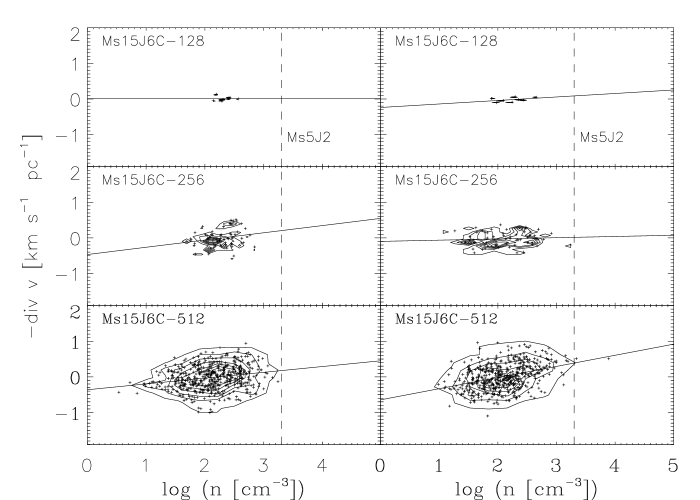
Figure 11: Negative mean velocity divergence versus mean density for subboxes of the large-scale simulation with compressible forcing, Ms15J6C, at the three resolutions we considered. The left-hand panels show the two-dimensional histograms of the subboxes in this plane at time $t=6$ Myr, before self-gravity is turned on, corresponding to 2 $t_{\rm turb}$ after the start of the simulations (left-hand panel). The right-hand panels show the histogram at $t=13.5$ Myr, corresponding to one free-fall time after gravity was turned on. The contours are drawn at increments of 1/7th of the maximum. The straight solid lines show least-squares fits through the data points. For the high-resolution run Ms15J6C-512, the fits have slopes $0.16\pm 0.031$ (left-hand panel) and $0.31\pm 0.034$ (right-hand panel), with correlation coefficients 0.22 and 0.38, respectively. The dashed vertical lines show the mean density of the small-scale simulation Ms5J2.

Figure 12: Fraction of mass accreted into collapsed objects as function of time in units of the free-fall time $t_{\rm ff}$ for the compressive-forcing simulations Ms15J6C-128, Ms15J6C-256, and Ms15J6C-512. The straight lines show least-squares fits to the accretion histories, with the indicated fitted slopes.

Figure 13: Left-hand panel: ${\rm SFE}_{\rm ff}$ for the various models assuming a fully compressible forcing ($b=1$) and $\alpha=0.475$, and the ${\rm SFE}_{\rm ff}$ for run Ms15J6C-512, with its associated 3$\sigma$ uncertainty. Right-hand panel: same as the middle panel, but with the model predictions calculated assuming $\alpha=4.75$.

4 Discussion

4.1 Comparison with previous work

4.1.1 Absence of simultaneously subsonic and super-Jeans structures, and the turbulent driving

Our result that no simultaneously subsonic and super-Jeans regions (either arbitrary subboxes of the simulations or dense cores) seem to appear in the simulations is qualitatively identical to our non-magnetic results from Paper I. In that paper, we speculated that the presence of the magnetic field might allow for the formation of subsonic, super-Jeans structures because of the ‘cushioning’ effect of the magnetic field, which might reduce the velocity difference between the converging flows that form the clumps. However, the fact that the absence of these structures persists suggests that, perhaps, the cushioning simultaneously causes the clumps to attain lower peak densities, with both effects tending to cancel each other out.

The absence of simultaneously subsonic and super-Jeans structures in our isothermal, driven-turbulence, magnetized simulations, in spite of their ubiquitous observed existence in actual molecular clouds, suggests that perhaps some other feature of our simulations is not sufficiently realistic. One possible candidate is the very nature of the velocity field in our simulations, which consists of randomly driven supersonic turbulence, in which the clumps are in fact the density fluctuations produced by the supersonic compressions in this turbulent regime, and the driving is applied at the largest scales in the numerical box. This continuous-driving setup is intended to model the turbulence driven into clouds and their substructure mostly by supernova explosions in the ambient ISM. Another important candidate is the isothermal effective equation of state, which is one of the assumptions we are testing, but which indeed may not be sufficiently realistic, since MCs may well contain a mixture of atomic and molecular gas phases (e.g., Li & Goldsmith, 2003).

Within this context, our three simulations, with their successively smaller physical scales, larger mean densities, and respective forcings applied at the largest scales available within each one, are intended to represent a hierarchy of nested turbulent density fluctuations. However, as already pointed out in Paper I, the equivalence between each run and a turbulent density fluctuation of the same size within a larger scale run is not perfect. While in each simulation the driving produces a zero net velocity divergence, Fig. 4 shows that this is not the case in high-density regions within run Ms15J6 that have the same size as run Ms5J2, as those regions tend to have, on average, a net velocity convergence. The same situation was encountered in Paper I. Moreover, it has recently been argued that the motions in numerical simulations of molecular cloud formation, even in the presence of stellar feedback, are dominated by hierarchical gravitational contraction (i.e. of collapses within collapses; Hoyle, 1953; Field et al., 2008; Vázquez-Semadeni et al., 2009), rather than by random, isotropic turbulence, again suggesting that the motions in the clouds are not equivalent to the random, supersonic turbulent we use in the present simulations, in spite of it being a standard procedure (for a recent example, see Federrath & Klessen, 2012). Moreover, there have been suggestions that this kind of simulations may produce cores that are systematically more dynamic than observed (André et al., 2009). In a future study, we plan to search for such structures in numerical simulations of hierarchical, chaotic gravitational contraction and fragmentation (e.g., Vázquez-Semadeni et al., 2007, 2011; Heitsch & Hartmann, 2008; Hennebelle et al., 2008; Banerjee et al., 2009; Heitsch et al., 2009; Clark et al., 2012).

4.1.2 The star formation efficiency per free-fall time

The values of the ${\rm SFE}_{\rm ff}$ obtained in Sec. 3.3, including the absence of collapse in run Ms5J2, can be compared with the non-magnetic results from Paper I. The values of ${\rm SFE}_{\rm ff}$ we obtained, of 0.002 for run Ms10J4 and of 0.034 for Ms15J6, are significantly smaller than those obtained for the corresponding runs in Paper I for the non-magnetic case, which were $\sim 0.11$ and $\sim 0.12$, respectively. The ${\rm SFE}_{\rm ff}$ for the present simulations, as well as for the non-magnetic runs from Paper I, are plotted as a function of ${\cal M}_{\rm s}$ in both panels of Fig. 7.

The strong reduction in the ${\rm SFE}_{\rm ff}$ observed in the magnetic runs indicates that the presence of a moderately supercritical magnetic field is able to strongly reduce the ${\rm SFE}_{\rm ff}$ when the magneto-thermal Jeans parameter (cf. Sec. 3.4) is sufficiently small, in agreement with previous results (e.g., Passot et al., 1995; Ostriker et al., 1999; Vázquez-Semadeni et al., 2005; Nakamura & Li, 2005; Price & Bate, 2008; Federrath & Klessen, 2012, 2013). The most dramatic difference occurs in the case of run Ms5J2, which in the magnetic case did not produce any collapse, at least for over four free-fall times (cf. Fig. 8). Instead, the corresponding non-magnetic run from Paper I had in fact the largest ${\rm SFE}_{\rm ff}$ of all runs in that paper. This implies that the combined thermal and magnetic support must be considered in order to determine the stability of a region since, as mentioned in Sec. 3.4, run M5J2 is diagnosed to be unstable by either the Jeans or the mass-to-flux criteria taken separately.

The ${\rm SFE}_{\rm ff}$ of our simulations can also be compared to the predictions from the theories by KM05, PN11, and HC11. A useful summary of the predictions from these theories, as well as simple extensions to the magnetic case, has been recently given by FK12. Specifically, the expressions for ${\rm SFE}_{\rm ff}$ as a function of the virial parameter $\alpha$, the rms Mach number, ${\cal M}_{\rm s}$, the plasma beta, $\beta$, and the forcing parameter, $b$ (which parametrizes the relative strength of compressible and solenoidal forcing) according to the three theories and to the multi-free-fall variant of each one, are given in Table 1 and equations 4, 31, and 39 of FK12. The assumed values of various parameters are described in sec. 2.5 of that paper, and we use the best-fitting values given in their table 3.

Some other parameters are characteristic of our simulations. Specifically, we use the nominal values of ${\cal M}_{\rm s}$ and $\beta$ for each run as indicated in our Table LABEL:tab:run_parameters, while, as explained in Sec. 2.2, all of our runs have a nominal value of $\alpha\approx 0.475$. Finally, since our main simulations use purely solenoidal forcing, we take $b=1/3$ (Federrath et al., 2008). It is important to note that FK12 warn that their proposed extension of the six theories to the magnetic case is applicable only for super-Alvénic flows, with ${\cal M}_{\rm A}\ga 2$. Since our simulations all have ${\cal M}_{\rm A}\approx 1$, they are slightly outside of the applicability range, and thus, moderate deviations are to be expected.

The predictions from all three theories, in both their original and ‘multi-free-fall’ modes (a total of six theoretical models), according to the expressions provided by FK12, are also plotted in Fig. 7, together with the values of the ${\rm SFE}_{\rm ff}$ derived from the simulations (cf. Sec. 3.3). The left panel-hand shows the results for the six theories in the non-magnetic (or ‘hydro’) case ($\beta\rightarrow\infty$) and for the simulations from Paper I, while the right-hand panel shows the magnetic (or MHD) case, for the values of $\beta$ corresponding to our runs (Table LABEL:tab:run_parameters). It is seen that, in general, both the magnitude of the ${\rm SFE}_{\rm ff}$ and its trend with ${\cal M}_{\rm s}$ is missed by the theoretical predictions. In the non-magnetic case, only the HC11 theory, in both its original and multi-free-fall forms, matches the magnitude of the simulation ${\rm SFE}_{\rm ff}$ for ${\cal M}_{\rm s}=5$, but not for ${\cal M}_{\rm s}=10$ and 15, since it predicts an increasing trend with ${\cal M}_{\rm s}$, while the simulations exhibit a globally decreasing trend. This trend is only predicted by the original KM05 theory which, however, is off in magnitude by nearly an order of magnitude. All other theories, including the multi-free-fall KM05 one, exhibit increasing trends with ${\cal M}_{\rm s}$.

In the magnetic case, we see that none of the theories, as modified by FK12 to include magnetic pressure, match the results from the simulations, neither in absolute magnitude of the ${\rm SFE}_{\rm ff}$ nor in the trend with ${\cal M}_{\rm s}$. In particular, while our simulations show a strong trend towards collapse suppression at lower ${\cal M}_{\rm s}$ with fixed $\alpha$, the theoretical models all tend to remain at roughly constant ${\rm SFE}_{\rm ff}$. This suggests that the procedure used by FK12 to include the magnetic field, consisting in simply substituting the sound speed by the sum in quadrature of the sound and the Alfvén speeds to determine the width of the density PDF and the effective Jeans length, does not capture the effect of the decrease of $J_{\rm eff}$ at low ${\cal M}_{\rm s}$ exhibited by our simulations.

This conclusion, however, cannot be considered as definitive since, as mentioned above, the Alvénic Mach number of our simulations, ${\cal M}_{\rm A}\approx 1$, is slightly outside the range of applicability of the magnetically extended theories, as stated by FK12 (${\cal M}_{\rm A}\ga 2$). However, it appears unlikely that a difference by a mere factor of 2 in the Alfvénic Mach number will change the behaviour in as drastic a manner as to go from complete collapse suppression to an independence of ${\rm SFE}_{\rm ff}$ from ${\cal M}_{\rm s}$, as shown in the right-hand panel of Fig. 7. Moreover, note that the values we have chosen for our parameters attempt to mimic the values observed in real regions of the size scales represented by the simulations. If anything, it can be argued that the magnetic field strength is somewhat excessive in the case of the larger scale simulations (Ms10J4 and Ms15J6). However, the chosen magnetic field strength appears to be typical for a region of mean density $n_{0}\sim 2000{\rm~{}cm}^{-3}$ (see, e.g. Crutcher et al., 2010), as is the case of run Ms5J2. Therefore, run Ms5J2 may be representative of real regions with the same physical conditions, even if it does not fall on the range of the applicability of the magnetically extended theories. In any case, further testing appears necessary in order to more precisely attest the accuracy of the theoretical models and their range of applicability.

4.2 Implications

Our results have important implications for our understanding of the role of turbulence in the support of, and regulation of SF in, molecular clouds. Our simulations have been set up to represent clouds obeying Larson’s (1981) linewidth–size and density–size scaling relations, so that all three of them have the same value of the virial parameter $\alpha$, and with the kinetic energy corresponding mostly to turbulent motions that counteract the cloud’s self gravity. For such a sequence of clouds, Krumholz & Tan (2007) have argued that, for a variety of molecular objects, the ${\rm SFE}_{\rm ff}$ is approximately constant, at a value ${\rm SFE}_{\rm ff}\sim$ 2%, independently of density, and thus, for clouds obeying both of equations (1) and (2), independently of Mach number as well. Note, however, that this conclusion by Krumholz & Tan (2007) is inconsistent with equation 30 of KM05, which is a fit to the numerical results from their theory and predicts, at constant $\alpha$, a scaling ${\rm SFE}_{\rm ff}\propto{\cal M}_{\rm s}^{-0.32}$, as also pointed out in section 3.2 of Elmegreen (2007).

In Paper I, we showed that our non-magnetic simulations were marginally consistent, within their uncertainties, with the ${\rm SFE}_{\rm ff}\sim{\cal M}_{\rm s}^{-0.32}$ dependence given by KM05. However, our magnetic simulations from this paper suggest that this dependence is strongly modified upon the introduction of a constant magnetic field strength, and in a way that does not agree with KM12’s extension of the KM05 theory to the magnetic case, nor with the other two theories, in neither of their variants. This disagreement may be attributed to the fact that the Alfvénic Mach number of our simulations ($\approx 1$ in all three runs) does not fall in the range where the extension to the magnetic case proposed by FK12 applies. On the other hand, since the required increment in our values of ${\cal M}_{\rm A}$ to fall in the applicability range is of only a factor of a few, it does not appear likely that the drastic observed discrepancy can be attributed to this.

5 Summary and conclusions

In this paper, we have presented numerical simulations of randomly driven, supersonic, magnetized, and isothermal turbulent flows, commonly believed to represent the flow within molecular clouds. Our simulations are the magnetized counterparts of the simulations presented in Paper I, and have allowed us, among other things, to determine whether, and to what extent, the conclusions reached in that paper extend to the magnetized case. Our main conclusions are as follows.

• We have used numerical simulations of continuously driven, isothermal turbulence as a sort of ‘reductio ad absurdum’ test of these hypotheses, showing that they lead to results that are inconsistent with the hypotheses. In particular, using random turbulent driving in a box causes the clumps to have a non-random flow, but rather having a net convergent component, so that the clumps cannot be modelled by a simple rescaled box with random driving.

• As in Paper I, we do not find any simultaneously subsonic and super-Jeans structures (neither regular subboxes of the numerical box nor dense clumps) in our simulations. In Paper I, we argued that perhaps our failure there to find such structures was due to the neglect of the magnetic field there, but the fact that we do not find them even in the magnetized case strongly suggests that they form only very rarely, if at all, in the kind of flows that we have simulated here, i.e., continuously and randomly driven, strongly supersonic, isothermal turbulent flow. On the other hand, since such structures are routinely observed in real molecular clouds (see, e.g. Goodman et al., 1998; Caselli et al., 2002; André et al., 2009), our result suggests that this type of flow may not be representative of the flow within molecular clouds. A viable alternative is the type of hierarchical, chaotic gravitational fragmentation, consisting of collapses within collapses, and seeded by turbulence, that has been discussed in other studies (e.g. Clark & Bonnell, 2005; Vázquez-Semadeni et al., 2009; Heitsch et al., 2009; Ballesteros-Paredes et al., 2011a), to which we plan to apply the same tests in a future study. Another viable alternative is that, rather than being isothermal, the flow in MCs may be thermally bistable, containing a mixture of atomic and molecular gas that may aid in the formation of these structures.

• Also as in Paper I, we have found that the turbulent density enhancements (‘clumps’) tend to have a net negative velocity divergence, although the typical magnitude of the convergence at a given overdensity is decreased with respect to the non-magnetic case. Nevertheless, the fact that this result persists indicates that a turbulent box with totally random turbulent velocity field (thus with a zero mean divergence) is not an exact match for the type of flow that develops inside the clumps, which contain a non-zero net velocity convergence.

  A crucial implication of the presence of a net convergent component in the non-thermal motion within the clumps is that the energy contained in these motions is not available for support against gravity, a fact which needs to be accounted for in theories relying on this support.

• Contrary to its non-magnetic counterpart in Paper I, which had the highest ${\rm SFE}_{\rm ff}$, run Ms5J2 did not produce any collapsing objects over more than four global free-fall times. We attributed this result to the fact that this run had the lowest value of the magneto-thermal Jeans parameter, $J_{\rm eff}$, among our simulations. Instead, run Ms15J6, which only had a value $J_{\rm eff}\sim 12\%$ larger than run Ms5J2, did not exhibit any delay in its development of collapsing regions compared to the non-magnetic case. Therefore, it appears that the transition from total to non-existent inhibition of the collapse is a very sharp function of this parameter. Of course, we cannot rule out the possibility that collapse will occur in run Ms5J2 after a sufficiently long time, but in any case, it can be concluded that the inhibition of gravitational collapse by the combined effect of thermal pressure and the magnetic field for this run is very strong.

• We compared the dependence of the ${\rm SFE}_{\rm ff}$ in our simulations (measured as the slope of the collapsed mass versus time in units of the free-fall time) on the turbulent Mach number ${\cal M}_{\rm s}$ against the predictions of the theories by KM05, PN11, and HC11, in both their original form, and as modified by FK12 to include the magnetic pressure (thus forming a set of six theoretical models in total). We compared our results against the analytic expressions provided by FK12 for each of the six models, finding that in general they fail to reproduce both the absolute magnitudes of the ${\rm SFE}_{\rm ff}$ we obtain, as well as the trend with ${\cal M}_{\rm s}$, in both the magnetic and non-magnetic cases. In particular, the suppression of collapse in run Ms5J2 is missed by all magnetic models.

• The failure of the theories in the magnetic case may be explained because the Alvénic Mach number of our simulations, ${\cal M}_{\rm A}\approx 1$, is too small by at least a factor of 2 to fall in the range where FK12 suggest their implementation of the effects of the magnetic field into the theories should apply. However, since the discrepancy between the predictions of the theories and the results of our simulations are large even at the qualitative level (complete suppression of collapse in the smallest, densest simulation), it is possible that the failure is an indication of a deeper problem with the theories.

• We suggest instead that the observed discrepancies in the magnitude of ${\rm SFE}_{\rm ff}$ and its dependence on ${\cal M}_{\rm s}$ originate from the fact that the assumptions of the theories are not verified in the flow realized in the simulations. First, the velocity field in subregions of the simulation is not a scaled-down version of the flow implemented in the simulations as a whole: while the latter is a fully random turbulent flow with zero net convergence, in subregions of the numerical boxes, the flow naturally develops, on average, a globally converging topology. This contradicts the assumption in the HC11 theory that, at each scale, turbulence provides additional support against collapse, since the converging component of the flow we have observed implies that at least a fraction of the kinetic energy collaborates with the collapse, rather than impeding it. Secondly, the KM05 and PN11 theories assume that the collapsing objects are clumps that are simultaneously subsonic and super-Jeans, while our simulations suggest that this is not the dominant collapse mechanism.

In conclusion, our results seem to cast doubt on the premises of the current SF theories and on simulations of randomly driven turbulence as accurate representations of the physical conditions in molecular clouds and their clumps. The fact that the motions in the clumps have a net convergent nature implies that, far from providing support against gravity, they will collaborate with it. Of course, as noted in Paper I, our analysis cannot discriminate between the convergent motions being produced by turbulence or gravity, and in reality it is likely that both agents contribute. In the near future, we plan to apply similar tests to a different kind of flow, suggested by numerical simulations of the formation and evolution of entire giant molecular clouds, in which the regime that develops seems to be dominated by gravity at all scales, and evolves through hierarchical, chaotic gravitational fragmentation.

Appendix A On the calculation of the virial parameter $\alpha$

Instead of the estimator given by equation (13), which is based on global flow parameters, FK12 have advocated using an estimator computed from the full computational domain, given by

$$\alpha=\frac{\displaystyle\sum_{i}M_{i}v_{i}^{2}}{\left|\displaystyle\sum_{i}M_{i}\phi_{i}\right|},$$ (16)

where $M_{i}$ is the mass of the $i$th cell, $v_{i}$ is the magnitude of the flow velocity in that cell, and $\phi_{i}$ is the gravitational potential there. FK12 argue that, because the flow develops highly inhomogeneous, irregularly shaped, and fractal-like density structures, this estimator better represents the potential generated by the actual density distribution.

However, some additional considerations are important as well. First is the issue that in a periodic box, the Poisson equation is actually computed as (see, e.g., Weinberg, 1972; Peebles, 1980; Alecian & Léorat, 1988)

$$\nabla^{2}\phi=4\pi G(\rho-\rho_{0}),$$ (17)

in order to avoid the well-known Jeans’ swindle; that is, the fact that the underlying equilibrium state in the Jeans gravitational instability analysis is only truly self-consistent when the mean density is zero. Equation (17) means that, in the simulations, the gravitational potential arises from the distribution of density fluctuations, rather than from the full density distribution.

In practice, this means that, in the simulation, underdense regions are characterized by positive values of the gravitational potential. In turn, this will cause the total sum of the gravitational term to be decreased, in fact explaining why FK12 obtained values of $\alpha$ up to an order of magnitude larger than that obtained with the global parameters. This is correct with respect to the simulations, although it reminds us that the large-scale gravitational potential in the simulations is somewhat unrealistic, especially if the simulation intends to represent an entire cloud. Its accuracy increases if the modelled region is intended to represent a small fraction of a much larger volume at the same mean density, as is the case, for example, of simulations of cloud formation within a much larger volume (e.g., Vázquez-Semadeni et al., 2007).

Secondly, the larger values of $\alpha$ obtained with the estimator (16) seem to accomplish the opposite result of FK12’s motivation to use it in the first place: the presence of large local density enhancements should result in a more tightly bound medium, which would in turn result in smaller values of $\alpha$, contrary to the larger values obtained from the estimator.

Moreover, in order to fully capture the binding of the local, dense structures, the local $\alpha$ parameter should be computed by taking the velocities referred to the local centres of mass of the clumps. In other words, if the intention of an $\alpha$ estimator is to reasonably represent local excursions to low values of $\alpha$, it must take into account not just the local value of the gravitational energy (the denominator), but also the local value of the kinetic energy (the numerator). But this must be done by removing the bulk velocity of a local density enhancement, a consideration that is not included in the estimator (16), and which in practice is very difficult to accomplish, because the average bulk velocity to subtract depends on the size scale of the clump.

The fact that FK12 tended to find larger, rather than smaller values of the $\alpha$ parameter when computing it directly from the simulation means that it was dominated by the effect of the modified Poisson equation, rather than by the presence of strong local density enhancements. Nevertheless, this is indeed more representative of the actual gravitational potential in the simulations, due to the modified form of the Poisson equation.

As a compromise, in the body of the paper, we compute the $\alpha$ parameter from the global parameters, but also show the predictions from the models when $\alpha$ is multiplied by a factor of 10, which is the maximum typical enhancement found by FK12, in order to obtain an estimate of the modification that can be expected to occur in the model predictions due to the computation of $\alpha$ directly from the simulations. In general, we find that the modifications are very small.

References

- André et al. (2009) André, P., Basu, S., & Inutsuka, S. 2009, Structure Formation in Astrophysics. Cambridge Univ. Press, Cambridge, p. 254
- Alecian & Léorat (1988) Alecian, G., & Léorat, J. 1988, A&A, 196, 1
- Ballesteros-Paredes et al. (2003) Ballesteros-Paredes, J., Klessen, R. S., & Vázquez-Semadeni, E. 2003, ApJ, 592, 188
- Ballesteros-Paredes et al. (2011a) Ballesteros-Paredes, J., Hartmann, L. W., Vázquez-Semadeni, E., Heitsch, F., & Zamora-Avilés, M. A. 2011, MNRAS, 411, 65
- Ballesteros-Paredes et al. (2011b) Ballesteros-Paredes, J., Vázquez-Semadeni, E., Gazol, A., et al. 2011, MNRAS, 416, 1436
- Banerjee et al. (2009) Banerjee, R., Vázquez-Semadeni, E., Hennebelle, P., & Klessen, R. S. 2009, MNRAS, 398, 1082
- Bertoldi & McKee (1992) Bertoldi, F., & McKee, C. F. 1992, ApJ, 395, 140
- Blitz (1993) Blitz, L. 1993, Protostars and Planets III, 125
- Bonazzola et al. (1987) Bonazzola, S., Heyvaerts, J., Falgarone, E., Perault, M., & Puget, J. L. 1987, A&A, 172, 293
- Brunt (2003) Brunt, C. M. 2003, ApJ, 584, 293
- Brunt et al. (2009) Brunt, C. M., Heyer, M. H., & Mac Low, M.-M. 2009, A&A, 504, 883
- Caselli & Myers (1995) Caselli, P., & Myers, P. C. 1995, ApJ, 446, 665
- Caselli et al. (2002) Caselli, P., Walmsley, C. M., Zucconi, A., Tafalla M., Dore L., Myers P. C., 2002, ApJ, 565, 331
- Chandrasekhar (1951) Chandrasekhar, S. 1951, Proc. R. Soc. A, 210, 26
- Clark & Bonnell (2005) Clark, P. C., & Bonnell, I. A. 2005, MNRAS, 361, 2
- Clark et al. (2012) Clark, P. C., Glover, S. C. O., Klessen, R. S., & Bonnell, I. A. 2012, MNRAS, 424, 2599
- Crutcher et al. (2010) Crutcher, R. M., Wandelt, B., Heiles, C., Falgarone, E., & Troland, T. H. 2010, ApJ, 725, 466
- Elmegreen (2007) Elmegreen, B. G. 2007, ApJ, 668, 1064
- Elmegreen & Scalo (2004) Elmegreen, B. G., & Scalo, J. 2004, ARAA, 42, 211
- Federrath & Klessen (2012) Federrath, C., & Klessen, R. S. 2012, ApJ, 761, 156 (FK12)
- Federrath & Klessen (2013) Federrath, C., & Klessen, R. S. 2013, ApJ, 763, 51
- Federrath et al. (2008) Federrath, C., Klessen, R. S., & Schmidt, W. 2008, ApJ, 688, L79
- Federrath et al. (2010) Federrath, C., Roman-Duval, J., Klessen, R. S., Schmidt, W., & Mac Low, M.-M. 2010, A&A, 512, A81
- Field et al. (2008) Field, G. B., Blackman, E. G., & Keto, E. R. 2008, MNRAS, 385, 181
- Gibson et al. (2009) Gibson, D., Plume, R., Bergin, E., Ragan, S., & Evans, N. 2009, ApJ, 705, 123
- Goldsmith & Arquilla (1985) Goldsmith, P. F., & Arquilla, R. 1985, Protostars and Planets II, Univ. Arizona Press, Tucson, AZ, p. 37
- Gómez et al. (2007) Gómez, G. C., Vázquez-Semadeni, E., Shadmehri, M., & Ballesteros-Paredes, J. 2007, ApJ, 669, 1042
- Goodman et al. (1993) Goodman, A. A., Benson, P. J., Fuller, G. A., & Myers, P. C. 1993, ApJ, 406, 528
- Goodman et al. (1998) Goodman, A. A., Barranco, J. A., Wilner, D. J., & Heyer, M. H. 1998, ApJ, 504, 223
- Heitsch & Hartmann (2008) Heitsch, F., & Hartmann, L. 2008, ApJ, 689, 290
- Heitsch et al. (2009) Heitsch, F., Ballesteros-Paredes, J., & Hartmann, L. 2009, ApJ, 704, 1735
- Hennebelle & Chabrier (2008) Hennebelle, P., & Chabrier, G. 2008, ApJ, 684, 395
- Hennebelle & Chabrier (2011) Hennebelle, P., & Chabrier, G. 2011, ApJ, 743, L29 (HC11)
- Hennebelle et al. (2008) Hennebelle, P., Banerjee, R., Vázquez-Semadeni, E., Klessen, R. S., & Audit, E. 2008, A&A, 486, L43
- Heyer et al. (2009) Heyer, M., Krawczyk, C., Duval, J., & Jackson, J. M. 2009, ApJ, 699, 1092
- Hopkins (2012a) Hopkins, P. F. 2012, MNRAS, 423, 2016
- Hopkins (2012b) Hopkins, P. F. 2012, MNRAS, 423, 2037
- Hopkins (2013) Hopkins, P. F. 2013, MNRAS, 430, 1653
- Hoyle (1953) Hoyle, F. 1953, ApJ, 118, 513
- Imara & Blitz (2011) Imara, N., & Blitz, L. 2011, ApJ, 732, 78
- Imara et al. (2011) Imara, N., Bigiel, F., & Blitz, L. 2011, ApJ, 732, 79
- Kegel (1989) Kegel, W. H. 1989, A&A, 225, 517
- Kim et al. (1999) Kim, J., Ryu, D., Jones, T. W., & Hong, S. S. 1999, ApJ, 514, 506
- Krumholz & McKee (2005) Krumholz, M. R., & McKee, C. F. 2005, ApJ, 630, 250 (KM05)
- Krumholz & Tan (2007) Krumholz, M. R., & Tan, J. C. 2007, ApJ, 654, 304
- Larson (1981) Larson, R. B. 1981, MNRAS, 194, 809
- Li & Goldsmith (2003) Li, D., & Goldsmith, P. F. 2003, ApJ, 585, 823
- Li et al. (2012) Li, J., Wang, J., Gu, Q., Zhang, Z.-y., & Zheng, X. 2012, ApJ, 745, 47
- McKee & Ostriker (2007) McKee, C. F., & Ostriker, E. C. 2007, ARAA, 45, 565
- Mac Low & Klessen (2004) Mac Low, M.-M., & Klessen, R. S. 2004, Rev. Mod. Phys., 76, 125
- Molina et al. (2012) Molina, F. Z., Glover, S. C. O., Federrath, C., & Klessen, R. S. 2012, MNRAS, 423, 2680
- Myers & Goodman (1988) Myers, P. C., & Goodman, A. A. 1988, ApJ, 326, L27
- Nakamura & Li (2005) Nakamura, F., & Li, Z.-Y. 2005, ApJ, 631, 411
- Nakano & Nakamura (1978) Nakano, T., & Nakamura, T. 1978, PASJ, 30, 671
- Ostriker et al. (1999) Ostriker, E. C., Gammie, C. F., & Stone, J. M. 1999, ApJ, 513, 259
- Padoan (1995) Padoan, P. 1995, MNRAS, 277, 377
- Padoan & Nordlund (2011) Padoan, P., & Nordlund, Å. 2011, ApJ, 730, 40 (PN11)
- Padoan et al. (1997) Padoan, P., Nordlund, A., & Jones, B. J. T. 1997, MNRAS, 288, 145
- Passot & Vázquez-Semadeni (1998) Passot, T., & Vázquez-Semadeni, E. 1998, Phys. Rev. E, 58, 4501
- Passot et al. (1995) Passot, T., Vazquez-Semadeni, E., & Pouquet, A. 1995, ApJ, 455, 536
- Peebles (1980) Peebles, P. J. E. 1980, Research supported by the National Science Foundation. Princeton University Press, Princeton, NJ,p. 435
- Phillips (1999) Phillips, J. P. 1999, A&AS, 134, 241
- Plume et al. (1997) Plume, R., Jaffe, D. T., Evans, N. J., II, Martin-Pintado, J., & Gomez-Gonzalez, J. 1997, ApJ, 476, 730
- Price & Bate (2008) Price, D. J., & Bate, M. R. 2008, MNRAS, 385, 1820
- Robertson & Goldreich (2012) Robertson, B., & Goldreich, P. 2012, ApJ, 750, L31
- Rosolowsky (2007) Rosolowsky, E. 2007, ApJ, 654, 240
- Scalo (1990) Scalo, J. 1990, in Capuzzo-Dolcetta R., Chiosi C., di Fazio A., eds, Astrophysics and Space Science Library, Vol. 162, Physical Processes in Fragmentation and Star Formation. Springer-Verlag, Berlin, p. 151
- Shirley et al. (2003) Shirley, Y. L., Evans, N. J., II, Young, K. E., Knez, C., & Jaffe, D. T. 2003, ApJS, 149, 375
- Shu (1992) Shu, F. H. 1992, Physics of Astrophysics, Vol. II. University Science Books, Mill Valley, CA
- Truelove et al. (1997) Truelove, J. K., Klein, R. I., McKee, C. F., Holliman J. H., II, Howell., Greenough J. A., 1997, ApJ, 489, L179
- Vázquez-Semadeni (1994) Vázquez-Semadeni, E. 1994, ApJ, 423, 681
- Vázquez-Semadeni & Gazol (1995) Vázquez-Semadeni, E., & Gazol, A. 1995, A&A, 303, 204
- Vázquez-Semadeni et al. (1996) Vázquez-Semadeni, E., Passot, T., & Pouquet, A. 1996, ApJ, 473, 881
- Vázquez-Semadeni et al. (1998) Vázquez-Semadeni, E., Cantó, J., & Lizano, S. 1998, ApJ, 492, 596
- Vázquez-Semadeni et al. (2000) Vázquez-Semadeni, E., Ostriker, E. C., Passot, T., Gammie, C. F., & Stone, J. M. 2000, Protostars and Planets IV. Univ. Arizona Press, Tucson, AZ, p. 3
- Vázquez-Semadeni et al. (2003) Vázquez-Semadeni, E., Ballesteros-Paredes, J., & Klessen, R. S. 2003, ApJ, 585, L131
- Vázquez-Semadeni et al. (2005) Vázquez-Semadeni, E., Kim, J., Shadmehri, M., & Ballesteros-Paredes, J. 2005, ApJ, 618, 344
- Vázquez-Semadeni et al. (2007) Vázquez-Semadeni, E., Gómez, G. C., Jappsen, A. K., Ballesteros-Paredes J., González R. F., Klessen R. S., 2007, ApJ, 657, 870
- Vázquez-Semadeni et al. (2008) Vázquez-Semadeni, E., González, R. F., Ballesteros-Paredes, J., Gazol, A., & Kim, J., 2008, MNRAS, 390, 769 (Paper I)
- Vázquez-Semadeni et al. (2009) Vázquez-Semadeni, E., Gómez, G. C., Jappsen, A.-K., Ballesteros-Paredes, J., & Klessen, R. S. 2009, ApJ, 707, 1023
- Vázquez-Semadeni et al. (2011) Vázquez-Semadeni, E., Banerjee, R., Gómez G. C., et al. 2011, MNRAS, 414, 2511
- Weinberg (1972) Weinberg, S. 1972, Gravitation and Cosmology: Principles and Applications of the General Theory of Relativity. Wiley New York, pp. 688, (ISBN 0-471-92567-5)
- Wu et al. (2010) Wu, J., Evans, N. J., Shirley, Y. L., & Knez, C. 2010, ApJS, 188, 313
- Zamora-Avilés et al. (2012) Zamora-Avilés, M., Vázquez-Semadeni, E., & Colín, P. 2012, ApJ, 751, 77
- Zuckerman & Evans (1974) Zuckerman, B., & Evans, N. J. 1974, ApJ, 192, L149