Robust bounds on risk-sensitive functionals via Rényi divergence

Rami Atar
Department of Electrical Engineering
Technion–Israel Institute of Technology
Haifa 32000, Israel
Research supported in part by the ISF (Grant 1349/08), the US-Israel BSF (Grant 2008466), and the Technion fund for promotion of research
   Kenny Chowdhary
Sandia National Laboratories
Livermore, CA 94550, USA
   Paul Dupuis
Division of Applied Mathematics
Brown University
Providence, RI 02912, USA
Research supported in part by the Department of Energy (DE-SC0002413,DE-SC0010539), the National Science Foundation (DMS-1317199), and the Air Force Office of Scientific Research (FA9550-12-1-0399).
Abstract

We extend the duality between exponential integrals and relative entropy to a variational formula for exponential integrals involving the Rényi divergence. This formula characterizes the dependence of risk-sensitive functionals and related quantities determined by tail behavior to perturbations in the underlying distributions, in terms of the Rényi divergence. The characterization gives rise to upper and lower bounds that are meaningful for all values of a large deviation scaling parameter, allowing one to quantify in explicit terms the robustness of risk-sensitive costs. As applications we consider problems of uncertainty quantification when aspects of the model are not fully known, as well their use in bounding tail properties of an intractable model in terms of a tractable one.

AMS subject classifications: 60F10, 60E15, 94A17

Keywords: Rényi divergence, risk-sensitive cost, rare events, large deviation, Laplace principle, robust bounds

1 Introduction

For many models encountered in engineering, the physical sciences, mathematical finance, and elsewhere, rare events play a key role in determining important properties of the system. Given a system model, large deviation theory can often be used to study the impact of rare events, and in particular can provide both qualitative and quantitative information [14, 10, 8, 23]. Of course large deviation theory provides only an asymptotic approximation, and so if non-asymptotic bounds are sought then one can appeal to other approximations such as Monte Carlo [2, 4, 12]. However, it is well known that the resulting estimates (both asymptotic and non-asymptotic) are sensitive to the underlying assumed distribution, owing to the fact that they are determined by tail properties of the distributions. As a consequence, understanding the impact of modeling errors and model uncertainty becomes especially important. Modeling uncertainty can take many forms. For example, for some parts of the system there may be justification for the use of distributions of a particular form, but with parameters that are not known precisely. For other parts of the system, however, there may not be a suitable probabilistic model, and one should instead assume only that parameters belong to some known set.

The present paper is concerned with probabilities associated with rare events and expected values that are largely determined by rare events. However, the issues just raised regarding model uncertainty and modeling error are also important for ordinary (e.g., order one) probabilities, and expected values that are not sensitive to rare events. For such problems, one can obtain tight bounds that hold for a well-defined family of “true” process models by computing certain functionals with respect to a given “nominal” model, and then using the duality between exponential integrals and relative entropy. For a detailed discussion we refer to [7]. Following standard terminology in the economics and control literature, we will refer to integrals of the form $\int_{S}e^{g}d\nu$ as risk-sensitive functionals, where $g:S\rightarrow\mathbb{R}$ is Borel measurable, $S$ is a Polish space, and $\nu$ a probability measure. The well-known duality alluded to above is

$$\log\int_{S}e^{g}d\nu=\sup_{\theta}\Big{[}\int_{S}gd\theta-R(\theta\|\nu)\Big{]},$$ (1.1)

where the supremum extends over all probability measures on $S$, and $R$ denotes relative entropy (see (2.2)). Based on this identity, the results of [7] give tight bounds on ordinary probabilities and expected values, i.e., quantities of the form $\int_{S}gd\theta$. The bounds are in terms of a maximum relative entropy distance between the nominal model, $\nu$, and a collection of models, $\theta$, which presumably include the true model, plus a risk-sensitive cost with respect to the nominal model. Note that the feasibility of explicit computation, which means computing or approximating exponential integrals, is thus linked to the choice of the nominal model. Robust properties of controls designed on a risk-sensitive criteria were first described in [11]. By considering suitable limits such criteria can be linked to other methods for handling model uncertainty, such as $H^{\infty}$ control [26].

As it turns out, the duality (1.1) is not useful for bounding expectations and analyzing problems with rare events, because the natural scaling properties are such that the probabilities and expected values of interest should themselves be expressed as risk-sensitive functionals (this point will be made precise later on). However, there is a generalization of relative entropy called Rényi relative entropy or Rényi divergence (introduced in [21]; see Section 2), with which risk-sensitive functionals can be expressed in terms of other risk-sensitive functionals. In particular, as we shall prove, the identities

$$\frac{1}{\beta}\log\int_{S}e^{\beta g}d\nu=\inf_{\theta}\Big{[}\frac{1}{\gamma}\log\int_{S}e^{\gamma g}d\theta+\frac{1}{\gamma-\beta}R_{\frac{\gamma}{\gamma-\beta}}(\nu\|\theta)\Big{]}$$ (1.2)

and

$$\frac{1}{\gamma}\log\int_{S}e^{\gamma g}d\nu=\sup_{\theta}\Big{[}\frac{1}{\beta}\log\int_{S}e^{\beta g}d\theta-\frac{1}{\gamma-\beta}R_{\frac{\gamma}{\gamma-\beta}}(\theta\|\nu)\Big{]}$$ (1.3)

hold for any $\beta,\gamma\in\mathbb{R}\setminus\{0\}$, $\beta<\gamma$, where for $\alpha\in\mathbb{R}\setminus\{0,1\}$ $R_{\alpha}$ denotes Rényi divergence of order $\alpha$ (see (2.1) and (2.3)). Moreover, (1.1) is a limit case of (1.3) as $\beta\rightarrow 0$, with $\gamma=1$. These identities make it possible to bound risk-sensitive functionals with respect to the true model, $\theta$, in terms of a risk-sensitive functional with respect to the nominal model $\nu$. In this paper we also give elementary examples of how these bounds can be used.

As mentioned previously, one must evaluate a risk sensitive functional with respect to a nominal model in order to turn the theoretical results into numerical bounds. This has implications and uses that go beyond assessing model uncertainty. In fact, it suggests an approach for bounding and approximating rare event probabilities when evaluation of this risk-sensitive functional is not possible or convenient for the known true model, by replacing it with the “closest” (in the sense of Rényi divergence) model for which the computation can be carried out, and then bounding the Rényi divergence between the nominal and true models. Examples illustrating this use will be given. One can generalize to problems of minimizing risk-sensitive costs with respect to a controlled process, and ask for robust bounds (i.e., bounds valid for a family of process models) in terms of the value function and optimal control for the nominal model. This would be analogous to the robust control of order one costs by using controls designed on the basis of risk-sensitive performance criteria [11], and will be considered elsewhere.

We are aware of two other variational formulas for which the convex duality relation (1.1) is a special case. The first is a duality formula for $\phi$-entropy ((2.60) in [18], (20) in [6]), which has played a central role in the study of concentration inequalities [18]. The other is a variational formula for the $f$-divergence (a notion similar to $\phi$-entropy), that has been used to develop $f$-divergence estimators based on independent and identically distributed (iid) samples from each of two given distributions. Such estimators are significant in learning problems such as classification, dimensionality reduction, and homogeneity testing (see [19], [22] for the variational formula and its uses). Although Rényi divergence is closely related to $f$-divergence (in particular, the former is a certain nonlinear transformation of the latter; see [17, 24]) it seems that the representation formulas (1.2) and (1.3) cannot be recovered from these variational characterizations. The issue of robustness for rare events and risk-sensitive functionals has not received a great deal of attention. A paper that does consider the topic is [16], which considers the impact of varying the underlying distributions on the form of the large deviation rate function and related minimizers.

The rest of the paper is organized as follows. In Section 2 we recall the definition and some properties of Rényi divergence, state the variational representations based on Rényi divergence and state some immediate consequences. Section 3 contains elementary applications to functionals of empirical measures of iid outcomes, queueing, and Brownian motion with drift, and Section 4 concludes with the proofs of the representation formulas.

2 Exponential integrals and Rényi divergence

2.1 Definition and properties of Rényi divergence

Let $({S},\mathcal{F})$ be a measurable space and let $\mathcal{P}=\mathcal{P}({S},\mathcal{F})$ denote the set of all probability measures on $({S},\mathcal{F})$. We say that a measure $\mu$ on $({S},\mathcal{F})$ dominates $\nu\in\mathcal{P}$ if $\nu$ is absolutely continuous with respect to $\mu$, and denote this by $\nu\ll\mu$. For two probability measures $\nu,\theta\in\mathcal{P}$, let $\nu^{\prime}=\frac{d\nu}{d\mu}$ and $\theta^{\prime}=\frac{d\theta}{d\mu}$ denote the Radon-Nikodym derivatives with respect to a dominating $\sigma$-finite measure $\mu$. For $\alpha>0$, $\alpha\neq 1$, the Rényi divergence of degree $\alpha$ of $\nu$ from $\theta$ is defined by (cf. [17])

$$R_{\alpha}(\nu\|\theta)\doteq\begin{cases}\infty&\text{if }\alpha>1\text{ and }\,\nu\not\ll\theta,\\ \displaystyle\frac{1}{\alpha(\alpha-1)}\log\int_{\{\nu^{\prime}\theta^{\prime}>0\}}\Big{(}\frac{\nu^{\prime}}{\theta^{\prime}}\Big{)}^{\alpha}d\theta&\text{otherwise.}\end{cases}$$ (2.1)

We follow [17] in defining $R_{\alpha}$ with the factor $\frac{1}{\alpha(\alpha-1)}$ rather than $\frac{1}{\alpha-1}$, which is also a common choice [3, 21, 24]. When $\nu$ and $\theta$ are mutually absolutely continuous, this expression can be written without reference to a dominating measure, namely

$$R_{\alpha}(\nu\|\theta)=\frac{1}{\alpha(\alpha-1)}\log\int_{S}\Big{(}\frac{d\nu}{d\theta}\Big{)}^{\alpha}d\theta=\frac{1}{\alpha(\alpha-1)}\log\int_{S}\Big{(}\frac{d\theta}{d\nu}\Big{)}^{1-\alpha}d\nu.$$

The definition of $R_{\alpha}$ is extended to $\alpha=1$ by letting $R_{1}=R$ be the relative entropy, or the Kullback-Liebler divergence, defined by

$$R(\nu\|\theta)\doteq\begin{cases}\infty&\text{if }\nu\not\ll\theta,\\ \displaystyle\int_{\{\nu^{\prime}\theta^{\prime}>0\}}\frac{\nu^{\prime}}{\theta^{\prime}}\log\frac{\nu^{\prime}}{\theta^{\prime}}d\theta&\text{otherwise.}\end{cases}$$ (2.2)

The definitions do not depend on the choice of the dominating measure, and since $\nu+\theta$ automatically dominates $\nu$ and $\theta$, $R_{\alpha}(\nu\|\theta)$ is well defined for all pairs $(\nu,\theta)\in\mathcal{P}^{2}$. For a proof of independence from the dominating measure as well as various properties of $R_{\alpha}$, see [15, 17, 24, 25]. To mention a few of these properties, let $\nu$ and $\theta$ be fixed. Then $\alpha\mapsto\alpha R_{\alpha}(\nu\|\theta)$ is nondecreasing as a map from $(0,\infty)$ to $[0,\infty]$, and continuous from the left (thus $R=\lim_{\alpha\uparrow 1}R_{\alpha}$). If $\nu$ and $\theta$ are mutually singular then $R_{\alpha}(\nu\|\theta)$ is infinite everywhere. Otherwise, it is finite and continuous on $(0,\bar{\alpha})$, where $\bar{\alpha}\doteq\sup\{\alpha:R_{\alpha}(\nu\|\theta)<\infty\}\geq 1$. Moreover, for every $\alpha>0$, $R_{\alpha}(\nu\|\theta)=0$ if and only if $\nu=\theta$.

A further useful property is the identity $R_{\alpha}(\nu\|\theta)=R_{1-\alpha}(\theta\|\nu)$, which holds for every $\alpha\in(0,1)$. We will use it to extend the definition of $R_{\alpha}$ to $\alpha\in\mathbb{R}\setminus\{0,1\}$. Namely, we set

$$R_{\alpha}(\nu\|\theta)\doteq R_{1-\alpha}(\theta\|\nu),\qquad\alpha<0.$$ (2.3)

This definition is consistent with the definition of $R_{\alpha}$, $\alpha\in\mathbb{R}$, given in (2.10) of [17], as follows from Remark 2.13 of [17].

2.2 Variational representations for exponential integrals

The variational representation for exponential integrals (1.1) is very closely related to the theory of large deviations, and in fact can serve as the natural starting point for the large deviations analysis of any system [9]. It also gives an inequality that allows for robust bounds on ordinary costs with respect to a “true” measure in terms of risk-sensitive costs for a “nominal” model plus relative entropy distance between the two. However, as noted in the Introduction, this variational representation does not seem to be useful when bounding risk-sensitive costs. The variational representations in Theorem 2.1 give useful bounds in that respect. A particular case of (2.4) appears in [13]. The proof of the theorem is given in Section 4.

Theorem 2.1

Let $\beta$ and $\gamma$ be members of $\mathbb{R}\setminus\{0\}$, with $\beta<\gamma$. Let $\nu\in\mathcal{P}$. Then for any bounded and measurable $g:S\rightarrow\mathbb{R}$, one has

$$\frac{1}{\beta}\log\int_{S}e^{\beta g}d\nu=\inf_{\theta\in\mathcal{P}}\Big{[}\frac{1}{\gamma}\log\int_{S}e^{\gamma g}d\theta+\frac{1}{\gamma-\beta}R_{\frac{\gamma}{\gamma-\beta}}(\nu\|\theta)\Big{]},$$ (2.4)

where the infimum is uniquely attained at $d\theta=e^{-(\gamma-\beta)g}d\nu/Z$, $Z=\int_{S}e^{-(\gamma-\beta)g}d\nu$. In addition,

$$\frac{1}{\gamma}\log\int_{S}e^{\gamma g}d\nu=\sup_{\theta\in\mathcal{P}}\Big{[}\frac{1}{\beta}\log\int_{S}e^{\beta g}d\theta-\frac{1}{\gamma-\beta}R_{\frac{\gamma}{\gamma-\beta}}(\theta\|\nu)\Big{]},$$ (2.5)

where the supremum is uniquely attained at $d\theta=e^{(\gamma-\beta)g}d\nu/Z$, $Z=\int_{S}e^{(\gamma-\beta)g}d\nu$.

Remark 2.2

Setting $\beta=\alpha-1$ and $\gamma=\alpha$ gives

$$\frac{1}{\alpha-1}\log\int_{S}e^{(\alpha-1)g}d\nu=\inf_{\theta\in\mathcal{P}}\Big{[}\frac{1}{\alpha}\log\int_{S}e^{\alpha g}d\theta+R_{\alpha}(\nu\|\theta)\Big{]},$$ (2.6)

and

$$\frac{1}{\alpha}\log\int_{S}e^{\alpha g}d\nu=\sup_{\theta\in\mathcal{P}}\Big{[}\frac{1}{\alpha-1}\log\int_{S}e^{(\alpha-1)g}d\theta-R_{\alpha}(\theta\|\nu)\Big{]},$$ (2.7)

for all $\alpha\neq 0$, $\alpha\neq 1$. Although (2.6) and (2.7) are special cases of (2.4) and (2.5), the latter can be recovered from the former (in fact with $\alpha$ in the range $\alpha>0$, $\alpha\neq 1$), as shown in the proof of Theorem 2.1. In most of what follows we will work with (2.6) and (2.7).

Remark 2.3

By taking the formal limit $\alpha\rightarrow 1$, we obtain from (2.6) the identity

$$\int_{S}gd\nu=\inf_{\theta\in\mathcal{P}}\Big{[}\log\int_{S}e^{g}d\theta+R(\nu\|\theta)\Big{]}$$

and from (2.7) the well-known convex duality formula (see [7, 9, 11])

$$\log\int_{S}e^{g}d\nu=\sup_{\theta\in\mathcal{P}}\Big{[}\int_{S}gd\theta-R(\theta\|\nu)\Big{]}.$$

Note that one can also take $\alpha\rightarrow 0$ in (2.6) and (2.7), in which case $\alpha R_{\alpha}(\nu\|\theta)\rightarrow-\log\theta(\nu^{\prime}>0)$, recovering the simple fact

$$0=\inf_{\theta\in\mathcal{P}}[-\log\theta(\nu^{\prime}>0)]=\sup_{\theta\in\mathcal{P}}\log\nu(\theta^{\prime}>0).$$

The main purpose of this paper is to observe the following inequalities that follow from (2.6) and (2.7), and to discuss how they can be used to study robustness of risk-sensitive functionals.

Corollary 2.4

Assume $\alpha>1$, $\theta\in\mathcal{P}$, $\nu\in\mathcal{P}$, and let $g:S\rightarrow\mathbb{R}$ be any measurable function. Then

$\displaystyle\frac{1}{\alpha-2}\log\int_{S}e^{(\alpha-2)g}d\nu-R_{\alpha-1}(\nu\|\theta)$ $\displaystyle\leq\frac{1}{\alpha-1}\log\int_{S}e^{(\alpha-1)g}d\theta$ (2.8)
$\displaystyle\leq\frac{1}{\alpha}\log\int_{S}e^{\alpha g}d\nu+R_{\alpha}(\theta\|\nu),$

where the first inequality also requires $\alpha>2$. Also, on the left hand side of (2.8) we interpret $\infty-\infty$ as $-\infty$.

See Section 4 for the proof. Similar inequalities can be deduced when $\alpha\in(0,1)$, but for our present purposes they do not seem to be particularly useful.

The following interpretation of Corollary 2.4 will be useful in the examples presented in the next section. By considering $g=0$ on $A\in\mathcal{F}$ and $g=-M$ on $A^{c}$, and then sending $M\rightarrow\infty$, one obtains that for any event $A$

$$\frac{1}{\alpha-2}\log\nu(A)-R_{\alpha-1}(\nu\|\theta)\leq\frac{1}{\alpha-1}\log\theta(A)\leq\frac{1}{\alpha}\log\nu(A)+R_{\alpha}(\theta\|\nu),$$ (2.9)

with the same restrictions on $\alpha$ as in the corollary.

3 Elementary applications

In this section we show how Corollary 2.4 can be used to provide robust bounds of the sort described in the Introduction. The examples are intended only to illustrate the main ideas, and limited to problems where the driving noises are distributed according to product measure. When assessing probabilities and expected values associated with rare events, it is important to keep in mind that it is usually relative errors, and not absolute errors, that are important. Also, it is generally the case that approximations are of an asymptotic nature as some scaling parameter tends to a limit. For light-tailed processes, the scaling is exponential in the parameter. As we will see, this fits in very nicely with the form of the inequalities in (2.8).

As described in the introduction, one should have in mind two scenarios. In one case, we think of $\theta$ as a probability measure of interest for which the large deviation functional may be hard to compute, and of $\nu$ as an alternative that is more tractable. In the other case we are not sure of the model, with the nominal model $\nu$ a sort of “best guess” and $\theta$ the true model.

3.1 Functionals of the empirical measure

Suppose that $S={\mathbb{R}}^{n}$, where $n$ is the scaling parameter. Let $\theta^{n}$ and $\nu^{n}$ be product probability measures on $S$, with marginals $\theta_{i}^{n}$ and $\nu_{i}^{n}$. Assume $\nu_{i}^{n}=\nu_{1}$, so the nominal model corresponds to an iid sequence. Then (cf. [15])

$${\Delta}_{\alpha}^{n}\doteq\frac{1}{n}R_{\alpha}(\theta^{n}\|\nu^{n})=\frac{1}{n}\sum_{i=1}^{n}R_{\alpha}(\theta_{i}^{n}\|\nu_{i}^{n})=\frac{1}{n}\sum_{i=1}^{n}R_{\alpha}(\theta_{i}^{n}\|\nu_{1}).$$

Let $X_{n}$ denote the canonical process. If the $X_{n}$ are also iid under $\theta^{n}$ with marginal $\theta_{1}$, then ${\Delta}_{\alpha}^{n}=R_{\alpha}(\theta_{1}\|\nu_{1})$ for every $n$. Consider the empirical measure $L_{n}=n^{-1}\sum_{i=1}^{n}\delta_{X_{i}}$ as a random element of the space $\mathcal{P}_{{\mathbb{R}}}=\mathcal{P}({\mathbb{R}},\mathcal{R})$, equipped with the topology of weak convergence, and fix any measurable function $G:\mathcal{P}\rightarrow{\mathbb{R}}$. Then with ${\mathbb{E}}_{\theta}$ and ${\mathbb{E}}_{\nu}$ denoting expectation with respect to the indicated distribution, we can take $g(X_{n})=nG(L_{n})$ in Corollary 2.4 to get

$$\frac{1}{n}\frac{1}{\alpha-1}\log{\mathbb{E}}_{\theta}e^{(\alpha-1)nG(L_{n})}\leq\frac{1}{n}\frac{1}{\alpha}\log{\mathbb{E}}_{\nu}e^{\alpha nG(L_{n})}+R_{\alpha}(\theta_{1}\|\nu_{1}).$$ (3.1)

(and also if desired a corresponding lower bound).

If $G$ is continuous and $\theta$ corresponds to an iid sequence, then in this very simple setting one could use Sanov’s theorem to evaluate the limit behavior of the two terms, and obtain

$$\frac{1}{\alpha-1}\sup_{\lambda\in\mathcal{P}_{{\mathbb{R}}}}[(\alpha-1)G(\lambda)-R(\lambda\|\theta_{1})]\leq\frac{1}{\alpha}\sup_{\lambda\in\mathcal{P}_{{\mathbb{R}}}}[\alpha G(\lambda)-R(\lambda\|\nu_{1})]+R_{\alpha}(\theta_{1}\|\nu_{1}).$$ (3.2)

The strength of the general inequalities based on Rényi divergence is that the bound (3.1) holds for all $n$, and moreover does not require that $\theta$ correspond to an iid sequence.

We can make (3.1) and (3.2) more concrete by considering, for example, Gaussian distributions $\theta_{1}=\mathcal{N}(\mu_{1},\sigma_{1}^{2})$ and $\nu_{1}=\mathcal{N}(\mu_{2},\sigma_{2}^{2})$. In this case

$$R_{\alpha}(\theta_{1}\|\nu_{1})=\begin{cases}\frac{1}{\alpha}\log\frac{\sigma_{2}}{\sigma_{1}}+\frac{1}{2\alpha(\alpha-1)}\log\frac{\sigma_{2}^{2}}{\sigma_{\alpha}^{2}}+\frac{1}{2\alpha}\frac{\alpha(\mu_{1}-\mu_{2})^{2}}{\sigma_{\alpha}^{2}},&\text{ if }\sigma_{\alpha}^{2}\doteq\alpha\sigma_{2}^{2}+(1-\alpha)\sigma_{1}^{2}>0,\\ \infty,&\text{ otherwise.}\end{cases}$$ (3.3)

If $G(L_{n})=c\langle 1,L_{n}\rangle=n^{-1}c(X_{1}+\cdots+X_{n})$ for some constant $c$ and $\nu_{1}=\mathcal{N}(0,1)$, then ${\mathbb{E}}_{\nu}e^{\alpha nG(L_{n})}={\mathbb{E}}_{\nu}e^{\alpha c(X_{1}+\cdots+X_{n})}=e^{\alpha^{2}c^{2}n/2}$ and (3.1) says that for every $\theta$ under which $X_{n}$ are iid,

$$\frac{1}{n}\frac{1}{\alpha-1}\log{\mathbb{E}}_{\theta}e^{(\alpha-1)c(X_{1}+\cdots+X_{n})}\leq R_{\alpha}(\theta_{1}\|\nu_{1})+\frac{\alpha c^{2}}{2}.$$ (3.4)

In (3.4) one obtains equality if $\theta$ is $\mathcal{N}(c,1)$, as can be verified using (3.3). As a result, (3.4) is tight in the following sense. Fix $\alpha>1$ and a constant $d>0$. Consider the family of $\theta_{1}$ for which $R_{\alpha}(\theta_{1}\|\nu_{1})\leq d$. With this notation, (3.4) states that for $\theta_{1}$ in this family,

$$\frac{1}{n}\frac{1}{\alpha-1}\log{\mathbb{E}}_{\theta}e^{(\alpha-1)c(X_{1}+\cdots+X_{n})}\leq d+\frac{\alpha c^{2}}{2}.$$

Moreover one can find $c$ and a $\theta_{1}$ in the family such that this display holds with equality. Indeed, $c$ is chosen so that $\frac{1}{2}(\alpha-1)c^{2}=d$ (namely, $c=\pm\sqrt{2d/(\alpha-1)}$) and $\theta_{1}=\mathcal{N}(c,1)$.

3.2 A sample path large deviation example

We next discuss a well-known example from queueing analysis. Lindley’s recursion

$$\begin{cases}Q_{n}=(Q_{n-1}+X_{n}-C)^{+},&n\geq 1,\\ Q_{0}=0,&\end{cases}$$

describes the queue length $Q_{n}$ in an initially empty queueing system where $X_{n}\geq 0$ arrivals occur at time $n\geq 1$, and the server is capable of serving $C$ customers at each time slot. Denoting $S_{0}=0$ and $S_{n}=X_{1}+\cdots+X_{n}$, the solution to this recursion is given by

$$Q_{n}=\max_{0\leq i\leq n}[S_{n}-S_{i}-Ci].$$

Assume that the system is stable in the sense that $C>{\mathbb{E}}_{\nu}[X_{1}]=1$. Consider the space-time rescaled processes $\bar{S}^{n}(t)=n^{-1}S_{[nt]}$ and $\bar{Q}^{n}(t)=n^{-1}Q_{[nt]}$, $t\geq 0$, and given a constant $b>0$, let the buffer overflow event be given by

$$A_{n}=\left\{\max_{t\in[0,1]}\bar{Q}^{n}(t)>b\right\}.$$

The large deviation asymptotic behavior of this sequence of events has been studied in general; see, for example, [1], and Section 11.7 of [23]. Here we will focus on a simple special case. Assume that under $\nu$, $X_{n}$ are iid standard Poisson. Let $\mathcal{AC}([0,1]:\mathbb{R})$ [resp., $\mathcal{D}([0,1]:\mathbb{R})$] denote the space of functions that are absolutely continuous [resp., right continuous with left limits] and that map $[0,1]$ to $\mathbb{R}$. Equip $\mathcal{D}([0,1]:\mathbb{R})$ with the Skorohod $J_{1}$ topology. The processes $\bar{S}^{n}$ are known to satisfy a sample-path large deviation principle in $\mathcal{D}([0,1]:\mathbb{R})$ with the rate function $I$ given by

$$I(\varphi)=\begin{cases}\int_{0}^{1}\ell(\dot{\varphi}(t))dt,&\text{if }\varphi\in\mathcal{AC}([0,1]:\mathbb{R}),\varphi(0)=0,\\ \infty,&\text{otherwise,}\end{cases}$$

where, with the convention $0\log 0=0$,

$$\ell(x)=\begin{cases}x\log x-x+1,&\text{if }x\geq 0,\\ \infty,&\text{if }x<0,\end{cases}$$

[20, Theorem 6.1(b)]. Hence $\lim_{n\rightarrow\infty}\frac{1}{n}\log\nu(A_{n})=-c$, where

$$c\doteq\inf\Big{\{}\int_{0}^{1}\ell(\dot{\varphi}(t))dt:\varphi\in\mathcal{AC},\varphi(0)=0,\max_{0\leq s\leq t\leq 1}\varphi(t)-\varphi(s)-C(t-s)\geq b\Big{\}}$$

can be found explicitly. Let $m^{\ast}$ and $t^{\ast}$ denote the minimum of $t\ell(C+\frac{b}{t})$ over $t>0$ and the unique minimizer, respectively. Then

$$c=\begin{cases}\ell(C+b)&\text{if }t^{\ast}\geq 1,\\ m^{\ast}&\text{if }t^{\ast}<1.\end{cases}$$

Note that the event $A_{n}$ depends only on $X_{1},\ldots,X_{n}$. If $\theta$ is any probability measure under which $X_{n}$ are iid and $R_{\alpha}(\theta_{1}\|\nu_{1})\leq d_{1}$ and $R_{\alpha-1}(\nu_{1}\|\theta_{1})\leq d_{2}$ for constants $d_{1},d_{2}$, then we obtain from (2.9) that for all $n$

$$\frac{1}{n}\frac{1}{\alpha-2}\log{\mathbb{P}}_{\nu}(A_{n})-d_{2}\leq\frac{1}{n}\frac{1}{\alpha-1}\log{\mathbb{P}}_{\theta}(A_{n})\leq\frac{1}{n}\frac{1}{\alpha}\log{\mathbb{P}}_{\nu}(A_{n})+d_{1},$$

or

$${\mathbb{P}}_{\nu}(A_{n})^{\frac{\alpha-1}{\alpha-2}}e^{n(\alpha-1)d_{2}}\leq{\mathbb{P}}_{\theta}(A_{n})\leq{\mathbb{P}}_{\nu}(A_{n})^{\frac{\alpha-1}{\alpha}}e^{n(\alpha-1)d_{1}}.$$

In particular,

$$-\frac{\alpha-1}{\alpha-2}c-(\alpha-1)d_{2}+o(1)\leq\frac{1}{n}\log\mathbb{P}_{\theta}(A_{n})\leq-\frac{\alpha-1}{\alpha}c+(\alpha-1)d_{1}+o(1),$$

as $n\rightarrow\infty$. More generally, the same conclusions hold if $\theta$ is any product measure under which

$$\frac{1}{n}\sum_{i=1}^{n}R_{\alpha}(\theta_{i}^{n}\|\nu_{1})\leq d_{1},\quad\frac{1}{n}\sum_{i=1}^{n}R_{\alpha-1}(\nu_{1}\|\theta_{i}^{n})\leq d_{2}.$$

3.3 Brownian motion with drift

Let $B_{t}$ be standard Brownian motion on $0\leq t\leq 1$ and let $P$ be the corresponding standard Wiener measure on $\mathcal{C}([0,1]:\mathbb{R})$. Let $Q$ be the measure induced by Brownian motion with constant drift, i.e.,

$$X_{t}=B_{t}+\mu t,$$

where $\mu\in\mathbb{R}$. Also, let $\tilde{Q}$ be the measure induced by the paths of the solution $X$ to the stochastic differential equation (SDE)

$$dX_{t}=m(X_{t})dt+dB_{t},\qquad X_{0}=0,$$

for measurable $m$, where, by assumption, weak existence and uniqueness hold. A simple calculation based on Girsanov’s theorem yields that the Rényi divergence between $Q$ and $P$ is given by

$$R_{\alpha}(Q\|P)=R_{\alpha}(P\|Q)=\frac{\mu^{2}}{2},$$ (3.5)

and that, if $|m(x)|\leq|\mu|$ for all $x$, then

$$R_{\alpha}(\tilde{Q}\|P)\leq\frac{\mu^{2}}{2},\qquad R_{\alpha}(P\|\tilde{Q})\leq\frac{\mu^{2}}{2}.$$ (3.6)

Let $A$ be the event that the path exceeds a certain level $K>0$:

$$A\doteq\left\{\omega:\sup_{0\leq t\leq 1}X_{t}>K\right\}.$$

The exceedance probability under the measure $Q$, which represents the probability of Brownian motion with constant drift exceeding $K$, is given (see [5, §2.1]) by

$$Q(A)=\frac{1}{2}\text{erfc}\left(\frac{K-\mu}{\sqrt{2}}\right)+\frac{1}{2}e^{2\mu K}\text{erfc}\left(\frac{K+\mu}{\sqrt{2}}\right),$$

where $\text{erfc}(x)=\frac{2}{\sqrt{\pi}}\int_{x}^{\infty}e^{-v^{2}}dv$, and under standard Wiener measure,

$$P(A)=\sqrt{\frac{2}{\pi}}\int_{K}^{\infty}e^{-x^{2}/2}dx=\text{erfc}\left(\frac{K}{\sqrt{2}}\right).$$ (3.7)

We would like to identify the bounds on $Q(A)$ and $\tilde{Q}(A)$ that Corollary 2.4 provides. In particular, by (2.9)

$$\frac{1}{\alpha-2}\log P(A)-R_{\alpha-1}(P\|Q)\leq\frac{1}{\alpha-1}\log Q(A)\leq\frac{1}{\alpha}\log P(A)+R_{\alpha}(Q\|P),$$

where the right hand side is valid for $\alpha>1$ and the left hand side is valid for $\alpha>2$. By (3.5) and (3.7) this gives

$$\frac{1}{\alpha-2}\log\text{erfc}\left(\frac{K}{\sqrt{2}}\right)-\frac{\mu^{2}}{2}\leq\frac{1}{\alpha-1}\log Q(A)\leq\frac{1}{\alpha}\log\text{erfc}\left(\frac{-K}{\sqrt{2}}\right)+\frac{\mu^{2}}{2},$$

or in probability scale

$$\text{erfc}\left(\frac{-K}{\sqrt{2}}\right)^{\frac{\alpha-1}{\alpha-2}}e^{-(\alpha-1)\frac{\mu^{2}}{2}}\leq Q(A)\leq\text{erfc}\left(\frac{-K}{\sqrt{2}}\right)^{\frac{\alpha-1}{\alpha}}e^{(\alpha-1)\frac{\mu^{2}}{2}}.$$

By (3.6), the same conclusion holds for $\tilde{Q}(A)$.

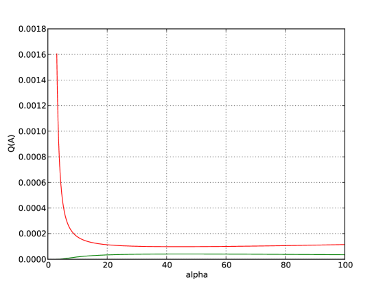
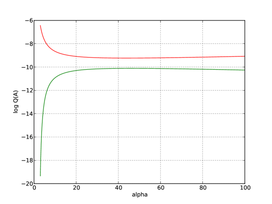
To illustrate these upper and lower bounds, we consider Brownian motion with constant drift with $|\mu|\leq.1$ so that $R_{\alpha}(P\|Q)\leq.005$ and $K=4$. Note that with $K=4$,

$$P(A)\approx 6.33\times 10^{-5}.$$

Figures 1 and 2 show the upper bounds in probability and log-probability scale, respectively, plotted as a function of $\alpha\in[3,100]$.

Refer to caption
Figure 1: Upper and lower bounds for $Q(A)$ in probability scale.
Refer to caption
Figure 2: Upper and lower bounds for $Q(A)$ in log probability scale.

As another example involving the measures $P$, $Q$ and $\tilde{Q}$, consider the random variable

$$H(t)=\inf\left\{s\in[0,t]:X_{s}=\sup_{u\in[0,t]}X_{u}\right\},\qquad t\geq 0.$$

The Laplace transform of $H(t)$ in the case of the standard Wiener measure is given by

$$\mathbb{E}_{P}[e^{-\gamma H(t)}]=e^{-\gamma t/2}I_{0}\left(\frac{\gamma t}{2}\right).$$

For the case of constant drift,

$$\mathbb{E}_{Q}[e^{-\gamma H(t)}]=\left(\frac{e^{-\gamma t-\mu^{2}t/2}}{\sqrt{\pi t}}+\frac{\mu e^{-\gamma t}}{\sqrt{2}}\text{erfc}\left(-\frac{\mu\sqrt{t}}{\sqrt{2}}\right)\right)\ast\left(\frac{e^{-\mu^{2}t/2}}{\sqrt{\pi t}}-\frac{\mu}{\sqrt{2}}\text{erfc}\left(\frac{\mu\sqrt{t}}{\sqrt{2}}\right)\right)$$

where $f(t)\ast g(t)$ denotes the convolution of $f$ and $g$ evaluated at $t$ (see [5]). There is no explicit expression for the case of a SDE. To obtain bounds on the behavior under $Q$ and $\tilde{Q}$ we apply Corollary 2.4, which gives

$\displaystyle\frac{1}{\alpha-2}\left[-\frac{(\alpha-2)\gamma t}{2}+\log I_{0}\left(\frac{(\alpha-2)\gamma t}{2}\right)\right]-\frac{\mu^{2}t}{2}$
$\displaystyle\hskip 80.00012pt\leq\frac{1}{\alpha-1}\log\mathbb{E}_{Q}[e^{(\alpha-1)\gamma H(t)}]$
$\displaystyle\hskip 80.00012pt\leq\frac{1}{\alpha}\left[-\frac{\alpha\gamma t}{2}+\log I_{0}\left(\frac{\alpha\gamma t}{2}\right)\right]+\frac{\mu^{2}t}{2}.$

As before, the same upper and lower bounds are valid for $\tilde{Q}$ as well.

4 Proofs of Theorem 2.1 and Corollary 2.4

Proof of Theorem 2.1. The main part of the proof will be to show the validity of (2.6) and (2.7) for all $\alpha>0$, $\alpha\neq 1$. Before proving these identities, let us show that they imply (2.4) and (2.5). First, note that (2.6) and (2.7) for $\alpha>0$, $\alpha\neq 1$ imply (2.6) and (2.7) for all $\alpha\in\mathbb{R}\setminus\{0,1\}$. Indeed, if $\alpha<0$ then (2.6) with $\bar{\alpha}=1-\alpha>1$ and $\bar{g}=-g$ reads

$$\frac{1}{\bar{\alpha}-1}\log\int e^{(\bar{\alpha}-1)\bar{g}}d\theta=\inf_{\theta\in\mathcal{P}}\Big{[}\frac{1}{\bar{\alpha}}\log\int e^{\bar{\alpha}\bar{g}}d\theta+R_{\bar{\alpha}}(\nu\|\theta)\Big{]}.$$

Expressed in terms of $\alpha$ and $g$,

$$-\frac{1}{\alpha}\log\int e^{\alpha g}d\theta=\inf_{\theta\in\mathcal{P}}\Big{[}-\frac{1}{\alpha-1}\log\int e^{(\alpha-1)g}d\theta+R_{\alpha}(\theta\|\nu)\Big{]},$$

where we used (2.3). Multiplying by $(-1)$ establishes the validity of (2.7) for $\alpha<0$. In a similar way, the validity of (2.6) for $\alpha<0$ follows from that of (2.7) for $\bar{\alpha}>1$.

Next, to show that (2.6) and (2.7) with $\alpha\in\mathbb{R}\setminus\{0,1\}$ imply (2.4) and (2.5), fix $\beta$ and $\gamma$ in $\mathbb{R}\setminus\{0\}$, $\beta<\gamma$. Apply (2.6) with $\alpha=\frac{\gamma}{\gamma-\beta}$ and $g=(\gamma-\beta)f$ (note that $\alpha\notin\{0,1\}$) and divide by $\gamma-\beta$ to get (2.4) (with $f$ in place of $g$). In a similar way, (2.5) follows from (2.7).

We turn to proving (2.6) for $\alpha>0$, $\alpha\neq 1$. Fix $\nu$, and consider first the case $\alpha>1$. Given any $\theta$, let $\mu=\mu(\theta)$ be a measure dominating both $\nu$ and $\theta$, and denote by $\nu^{\prime}$ and $\theta^{\prime}$ the corresponding densities. Define $\lambda\in\mathcal{P}$ by $d\lambda=e^{-g}d\nu/Z$ where $Z=\int_{S}e^{-g}d\nu$, and let $\lambda^{\prime}$ be the density of $\lambda$ with respect to $\mu$. First suppose that $\theta$ dominates $\nu$. Then $\lambda^{\prime}/\nu^{\prime}=e^{-g}/Z$, and so

$\displaystyle\log\int_{S}e^{\alpha g}d\theta$ $\displaystyle\geq\log\int_{\{\nu^{\prime}>0\}}e^{\alpha g}d\theta$ (4.1)
$\displaystyle=\log\int_{\{\nu^{\prime}>0\}}\frac{1}{Z}\frac{\nu^{\prime}}{\lambda^{\prime}}e^{(\alpha-1)g}d\theta$
$\displaystyle=\log\int_{S}\frac{1}{Z}\frac{\nu^{\prime}\theta^{\prime}}{\lambda^{\prime}}e^{(\alpha-1)g}d\mu$
$\displaystyle=\log\int_{S}\frac{1}{Z}\frac{\theta^{\prime}}{\lambda^{\prime}}e^{(\alpha-1)g}d\nu.$

Moreover, since $\nu\ll\theta$ $\mu\{\nu^{\prime}\theta^{\prime}>0\}=\mu\{\nu^{\prime}>0\}$, and therefore

$\displaystyle R_{\alpha}(\nu\|\theta)$ $\displaystyle=\frac{1}{\alpha(\alpha-1)}\log\int_{\{\nu^{\prime}\theta^{\prime}>0\}}\Big{(}\frac{\nu^{\prime}}{\theta^{\prime}}\Big{)}^{\alpha}d\theta$
$\displaystyle=\frac{1}{\alpha(\alpha-1)}\log\int_{\{\nu^{\prime}>0\}}\Big{(}\frac{\nu^{\prime}}{\theta^{\prime}}\Big{)}^{\alpha-1}d\nu$
$\displaystyle=\frac{1}{\alpha(\alpha-1)}\log\int_{\{\nu^{\prime}>0\}}Z^{\alpha-1}\Big{(}\frac{\lambda^{\prime}}{\theta^{\prime}}\Big{)}^{\alpha-1}e^{(\alpha-1)g}d\nu.$

Thus with $d\tilde{\nu}=e^{(\alpha-1)g}d\nu$,

$$\frac{1}{\alpha}\log\int_{S}e^{\alpha g}d\theta+R_{\alpha}(\nu\|\theta)\geq\frac{1}{\alpha}\log\int_{S}\frac{\theta^{\prime}}{\lambda^{\prime}}d\tilde{\nu}+\frac{1}{\alpha(\alpha-1)}\log\int_{\{\nu^{\prime}>0\}}\Big{(}\frac{\lambda^{\prime}}{\theta^{\prime}}\Big{)}^{\alpha-1}d\tilde{\nu}.$$ (4.2)

On the set $\{\nu^{\prime}>0\}=\{\lambda^{\prime}\theta^{\prime}>0\}$, define

$$\varphi=\Big{(}\frac{\lambda^{\prime}}{\theta^{\prime}}\Big{)}^{\frac{\alpha-1}{\alpha}},\qquad\psi=\Big{(}\frac{\theta^{\prime}}{\lambda^{\prime}}\Big{)}^{\frac{\alpha-1}{\alpha}},$$

so that $\varphi\psi=1$ on $\{\nu^{\prime}>0\}$. By Hölder’s inequality with $1/p=1/\alpha$ and $1/q=(\alpha-1)/\alpha$, and with $p$ attached to $\varphi$ and $q$ attached to $\psi$, we have

$$\int_{S}d\tilde{\nu}\leq\Big{(}\int_{\{\nu^{\prime}>0\}}\Big{(}\frac{\lambda^{\prime}}{\theta^{\prime}}\Big{)}^{\alpha-1}d\tilde{\nu}\Big{)}^{\frac{1}{\alpha}}\Big{(}\int_{S}\frac{\theta^{\prime}}{\lambda^{\prime}}d\tilde{\nu}\Big{)}^{\frac{\alpha-1}{\alpha}}.$$ (4.3)

Taking logs, dividing by $\alpha-1$ and using (4.2) gives that for any $\theta\in\mathcal{P}$ with $\theta\gg\nu$,

$$\frac{1}{\alpha}\log\int_{S}e^{\alpha g}d\theta+R_{\alpha}(\nu\|\theta)\geq\frac{1}{\alpha-1}\log\int_{S}d\tilde{\nu}=\frac{1}{\alpha-1}\log\int_{S}e^{(\alpha-1)g}d\nu.$$

If $\nu\not\ll\theta$ then $R_{\alpha}(\nu\|\theta)=\infty$, and again the inequality holds.

Taking the infimum over all $\theta\in\mathcal{P}$ shows that the right hand side of (2.6) is bounded below by the left hand side. Note that since $g$ is bounded $\lambda\{\nu^{\prime}>0\}=\lambda\{S\}$. Thus the choice $\theta=\lambda$ gives equality in both (4.1) and (4.3), hence in (2.6), and therefore identifies a minimizer.

Finally we show that the minimizer is unique. Assume that $\theta\gg\nu$ attains the infimum over $\mathcal{P}$. Then both (4.1) and (4.3) must hold with equality. For (4.1) to hold with equality, $\theta\sim\nu$ must be true. Recall that Hölder’s inequality will give an equality if and only if $\theta^{\prime}/\lambda^{\prime}$ is constant on $\{\nu^{\prime}>0\}=\{\lambda^{\prime}>0\}$. The only probability measure that satisfies these conditions is $\theta=\lambda$, which shows that $\lambda$ attains the infimum uniquely.

Next we consider (2.6) for the same $\nu$, but for $\alpha\in(0,1)$. In this case, we can no longer assume $\theta\gg\nu$. To show that the left hand side of (2.6) is a lower bound for the right hand side, consider any $\theta\in\mathcal{P}$. As with the case $\alpha>1$, let $\mu$ be a measure dominating both $\nu$ and $\theta$, and define $\nu^{\prime},\theta^{\prime}$ and $\lambda^{\prime}$ with respect to this measure, where $d\lambda=e^{-g}d\nu/Z$. Starting with the right hand side of (2.6),

$\displaystyle\log\int_{S}e^{\alpha g}d\theta$ $\displaystyle\geq\log\int_{\{\nu^{\prime}\theta^{\prime}>0\}}e^{\alpha g}d\theta$ (4.4)
$\displaystyle=\log\int_{\{\nu^{\prime}\theta^{\prime}>0\}}\frac{1}{Z}\frac{\theta^{\prime}}{\lambda^{\prime}}e^{(\alpha-1)g}d\nu,$

and

$\displaystyle R_{\alpha}(\nu\|\theta)$ $\displaystyle=\frac{1}{\alpha(\alpha-1)}\log\int_{\{\nu^{\prime}\theta^{\prime}>0\}}\Big{(}\frac{\nu^{\prime}}{\theta^{\prime}}\Big{)}^{\alpha}d\theta$
$\displaystyle=\frac{1}{\alpha(\alpha-1)}\log\int_{\{\nu^{\prime}\theta^{\prime}>0\}}Z^{\alpha-1}\Big{(}\frac{\lambda^{\prime}}{\theta^{\prime}}\Big{)}^{\alpha-1}e^{(\alpha-1)g}d\nu.$

With $\tilde{\nu}$ again defined by $d\tilde{\nu}=e^{(\alpha-1)g}d\nu$,

$$\frac{1}{\alpha}\log\int_{S}e^{\alpha g}d\theta+R_{\alpha}(\nu\|\theta)\geq\frac{1}{\alpha}\log\int_{\{\nu^{\prime}\theta^{\prime}>0\}}\frac{\theta^{\prime}}{\lambda^{\prime}}d\tilde{\nu}+\frac{1}{\alpha(\alpha-1)}\log\int_{\{\nu^{\prime}\theta^{\prime}>0\}}\Big{(}\frac{\lambda^{\prime}}{\theta^{\prime}}\Big{)}^{\alpha-1}d\tilde{\nu}.$$ (4.5)

Define $\varphi=1$ and $\psi=(\lambda^{\prime}/\theta^{\prime})^{\alpha-1}$ on the set $\{\nu^{\prime}\theta^{\prime}>0\}$. Using Hölder’s inequality with $p=1/\alpha$ attached to $\varphi$ and $q=1/(1-\alpha)$ attached to $\psi$ gives

$$\int_{\{\nu^{\prime}\theta^{\prime}>0\}}\Big{(}\frac{\lambda^{\prime}}{\theta^{\prime}}\Big{)}^{\alpha-1}d\tilde{\nu}\leq\Big{(}\int_{\{\nu^{\prime}\theta^{\prime}>0\}}d\tilde{\nu}\Big{)}^{\alpha}\Big{(}\int_{\{\nu^{\prime}\theta^{\prime}>0\}}\frac{\theta^{\prime}}{\lambda^{\prime}}d\tilde{\nu}\Big{)}^{1-\alpha}.$$

Taking logs and dividing by $\alpha(\alpha-1)<0$ gives

$$\frac{1}{\alpha(\alpha-1)}\log\int_{\{\nu^{\prime}\theta^{\prime}>0\}}\Big{(}\frac{\lambda^{\prime}}{\theta^{\prime}}\Big{)}^{\alpha-1}d\tilde{\nu}\geq\frac{1}{\alpha-1}\log\int_{\{\nu^{\prime}\theta^{\prime}>0\}}d\tilde{\nu}-\frac{1}{\alpha}\log\int_{\{\nu^{\prime}\theta^{\prime}>0\}}\frac{\theta^{\prime}}{\lambda^{\prime}}d\tilde{\nu}.$$

Using (4.5) gives

$\displaystyle\frac{1}{\alpha}\log\int_{S}e^{\alpha g}d\theta+R_{\alpha}(\nu\|\theta)$ $\displaystyle\geq\frac{1}{\alpha-1}\log\int_{\{\nu^{\prime}\theta^{\prime}>0\}}d\tilde{\nu}$
$\displaystyle=\frac{1}{\alpha-1}\log\int_{\{\nu^{\prime}\theta^{\prime}>0\}}e^{(\alpha-1)g}d\nu$
$\displaystyle\geq\frac{1}{\alpha-1}\log\int_{S}e^{(\alpha-1)g}d\nu,$ (4.6)

showing that (2.6) holds as an inequality. To show equality, substitute $\lambda$ for $\theta$ and note that all the inequalities hold as equalities.

To show that $\lambda$ is the unique minimizer, note that any $\theta\in\mathcal{P}$ satisfying all inequalities as equalities, must, in particular, give equality in (4.4), for which it is necessary that $\theta\ll\nu$. Equality in (4.6) implies $\nu\ll\theta$. For Hölder’s inequality to hold with equality $\psi$ must be a constant, and the only probability measure satisfying these conditions is $\lambda$. This completes the proof of (2.6).

Toward proving (2.7), note that (2.6) implies

$$\frac{1}{\alpha-1}\log\int_{S}e^{(\alpha-1)g}d\nu\leq\frac{1}{\alpha}\log\int_{S}e^{\alpha g}d\theta+R_{\alpha}(\nu\|\theta),\qquad\nu,\theta\in\mathcal{P},$$

which is equivalent to

$$\frac{1}{\alpha}\log\int_{S}e^{\alpha g}d\nu\geq\frac{1}{\alpha-1}\log\int_{S}e^{(\alpha-1)g}d\theta-R_{\alpha}(\theta\|\nu),\qquad\nu,\theta\in\mathcal{P}.$$

Thus to prove part (2.7), it suffices to show that the measure $d\theta=e^{g}d\nu/Z$, and only this measure, gives equality in the above display. The proof is similar to that of (2.6), and therefore the details are omitted.


Proof of Corollary 2.4. We give a proof of only the rightmost inequality; the other inequality is proved analogously. First, if $g$ is bounded the result follows from Theorem 2.1. Otherwise, since the claim holds trivially if the right hand side is infinite, assume it is finite. Let $g^{M,N}=(g\vee-M)\wedge N$, for $M,N\geq 0$. Then

$$\frac{1}{\alpha-1}\log\int_{S}e^{(\alpha-1)g^{M,N}}d\theta\leq\frac{1}{\alpha}\log\int_{S}e^{\alpha g^{M,N}}d\nu+R_{\alpha}(\theta\|\nu).$$ (4.7)

We first take $M\rightarrow\infty$ and use dominated convergence on both sides of the inequality. To this end note that $g^{M,N}\leq g^{+}$. Since $R_{\alpha}(\theta\|\nu)\geq 0$ it must be true that $e^{\alpha g}$ is $\nu$-integrable, and therefore so is $e^{\alpha g^{+}}$. Moreover, for fixed $N$, $g^{M,N}\leq g^{0,N}$ and, using (4.7) with $M=0$, shows that $e^{(\alpha-1)g^{0,N}}$ is $\theta$-integrable. As a result, (4.7) holds with $g^{\infty,N}$ on both sides. Now we take $N\rightarrow\infty$ and use monotone convergence (recall that $\alpha>1$). This gives the rightmost inequality in (2.8) and completes the proof.


Acknowledgment. We are grateful to Ramon van Handel for bringing to our attention the dualities in [6] and [18].


References

  • [1] V. Anantharam. How large delays build up in a $GI/G/1$ queue. Queueing Systems Theory Appl., 5(4):345–367, 1989.
  • [2] S. Asmussen and P.W. Glynn. Stochastic Simulation: Algorithms and Analysis. Applications of Mathematics. Springer Science+Business Media, LLC, 2007.
  • [3] A. Bhattacharyya. On some analogues of the amount of information and their use in statistical estimation. Sankhyā, 8:1–14, 1946.
  • [4] J.H. Blanchet and P. Glynn. Efficient rare-event simulation for the maximum of heavy-tailed random walks. Ann. Appl. Prob., 18:1351–1378, 2008.
  • [5] A. N. Borodin and P. Salminen. Handbook of Brownian motion—facts and formulae. Probability and its Applications. Birkhäuser Verlag, Basel, second edition, 2002.
  • [6] D. Chafaï. Entropies, convexity, and functional inequalities: on $\Phi$-entropies and $\Phi$-Sobolev inequalities. J. Math. Kyoto Univ., 44(2):325–363, 2004.
  • [7] K. Chowdhary and P. Dupuis. Distinguishing and integrating aleatoric and epistemic variation in uncertainty quantification. ESAIM: Mathematical Modelling and Numerical Analysis, 47:635–662, 2013.
  • [8] A. Dembo and O. Zeitouni. Large Deviations Techniques and Applications. Jones and Bartlett, Boston, 1993.
  • [9] P. Dupuis and R. S. Ellis. A Weak Convergence Approach to the Theory of Large Deviations. John Wiley & Sons, New York, 1997.
  • [10] P. Dupuis and R.S. Ellis. Large deviations for Markov processes with discontinuous statistics, II: Random walks. Probab. Th. Rel. Fields, 91:153–194, 1992.
  • [11] P. Dupuis, M. R. James, and I. R. Petersen. Robust properties of risk–sensitive control. Math. Control Signals Systems, 13:318–332, 2000.
  • [12] P. Dupuis and H. Wang. Subsolutions of an Isaacs equation and efficient schemes for importance sampling. Math. Oper. Res., 32:1–35, 2007.
  • [13] K. Dvijotham and E. Todorov. A unified theory of linearly solvable optimal control. Artificial Intelligence (UAI), page 1, 2011.
  • [14] M. I. Freidlin and A. D. Wentzell. Random Perturbations of Dynamical Systems. Springer-Verlag, New York, 1984.
  • [15] L. Golshani, E. Pasha, and G. Yari. Some properties of Rényi entropy and Rényi entropy rate. Inform. Sci., 179(14):2426–2433, 2009.
  • [16] H. J. Kushner. Robustness and approximation of escape times and large deviations estimates for systems with small noise effects. SIAM J. Appl. Math., 44:160–182, 1984.
  • [17] F. Liese and I. Vajda. Convex Statistical Distances. Teubner-Texte zur Mathematik. Teubner, 1987.
  • [18] P. Massart. Concentration inequalities and model selection, volume 1896 of Lecture Notes in Mathematics. Springer, Berlin, 2007. Lectures from the 33rd Summer School on Probability Theory held in Saint-Flour, July 6–23, 2003, With a foreword by Jean Picard.
  • [19] X. Nguyen, H.J. Wainwright, and M.I. Jordan. Estimating divergence functionals and the likelihood ratio by convex risk minimization. IEEE Trans. Inform. Theory, 56(11):5847–5861, 2010.
  • [20] A.A. Puhalskii and W. Whitt. Functional large deviation principles for first-passage-time processes. Ann. Appl. Probab., 7(2):362–381, 1997.
  • [21] A. Rényi. On measures of entropy and information. In Proc. 4th Berkeley Sympos. Math. Statist. and Prob., Vol. I, pages 547–561, Berkeley, Calif., 1961. Univ. California Press.
  • [22] A. Ruderman, M. Reid, D. García-García, and J. Petterson. Tighter variational representations of f-divergences via restriction to probability measures. arXiv preprint arXiv:1206.4664, 2012.
  • [23] A. Shwartz and A. Weiss. Large Deviations for Performance Analysis: Queues, Communication and Computing. Chapman and Hall, New York, 1995.
  • [24] I. Vajda. Distances and discrimination rates for stochastic processes. Stochastic Process. Appl., 35:47–57, 1990.
  • [25] T. van Erven and P. Harremoës. Rényi divergence and majorization. In Information Theory Proceedings (ISIT), 2010 IEEE International Symposium on, pages 1335–1339. IEEE, 2010.
  • [26] P. Whittle. Risk–sensitive linear/quadratic/guassian control. Adv. Appl. Prob., 13:777–784, 1981.