Narrow Band X-ray Photometry as a Tool for Studying Galaxy and Cluster Mass Distributions

Abstract

We explore the utility of narrow band X-ray surface photometry as a tool for making fully Bayesian, hydrostatic mass measurements of clusters of galaxies, groups and early-type galaxies. We demonstrate that it is sufficient to measure the surface photometry with the Chandra X-ray observatory in only three (rest frame) bands (0.5–0.9 keV, 0.9–2.0 keV and 2.0–7.0 keV) in order to constrain the temperature, density and abundance of the hot interstellar medium (ISM). Adopting parametrized models for the mass distribution and radial entropy profile and assuming spherical symmetry, we show that the constraints on the mass and thermodynamic properties of the ISM that are obtained by fitting data from all three bands simultaneously are comparable to those obtained by fitting similar models to the temperature and density profiles derived from spatially resolved spectroscopy, as is typically done. We demonstrate that the constraints can be significantly tightened when exploiting a recently derived, empirical relationship between the gas fraction and the entropy profile at large scales, eliminating arbitrary extrapolations at large radii. This “Scaled Adiabatic Model” (ScAM) is well suited to modest signal-to-noise data, and we show that accurate, precise measurements of the global system properties are inferred when employing it to fit data from even very shallow, snapshot X-ray observations. The well-defined asymptotic behaviour of the model also makes it ideally suited for use in Sunyaev-Zeldovich studies of galaxy clusters.

1 Introduction

The distribution of mass in galaxy clusters, groups and massive galaxies provides a powerful tool for cosmological studies. Explicit predictions from our current $\Lambda$CDM cosmological paradigm for the number, size and radial mass distribution of dark matter halos can now be tested against high-quality constraints from studies employing lensing, Sunyaev-Zeldovich, stellar dynamics and, in particular, X-rays (e.g. Voit & Donahue, 2005; Buote et al., 2007; Mahdavi et al., 2007; Gebhardt & Thomas, 2009; Vikhlinin et al., 2009; Okabe et al., 2010; Planck Collaboration et al., 2011). The relative distribution of dark and baryonic mass, coupled with the thermodynamic state of the hot intracluster medium, similarly provides a unique insight into the uncertain baryonic physics of galaxy formation, such as the role of feedback in shaping the nascent structures, and the complex interplay between adiabatic contraction and dynamical friction (e.g. Silk & Rees, 1998; Gnedin et al., 2004; Hopkins et al., 2006; Abadi et al., 2010).

Spherical, hydrostatic X-ray techniques are an appealing method for measuring such mass distributions due to their computational simplicity, given the isotropy of the gas pressure tensor, and the small biases introduced by the spherical approximation (Buote & Humphrey, 2012c, and references therein), particularly if the spherically averaged mass profile is close to a singular isothermal sphere (Buote & Humphrey, 2012b; Churazov et al., 2008). While the hot gas permeating the potential well is not expected to be exactly hydrostatic, theoretical arguments and observational constraints suggest only modest ($\mathrel{\hbox to0.0pt{\lower 3.0pt\hbox{$\sim$}\hss}\raise 2.0pt\hbox{$<$}}$ 30%) biases on the inferred gravitating mass distribution, provided care is taken to study systems with relaxed X-ray morphologies (e.g. Buote & Tsai, 1995; Evrard et al., 1996; Allen, 1998; Nagai et al., 2007; Piffaretti & Valdarnini, 2008; Churazov et al., 2008; Mahdavi et al., 2008; Fang et al., 2009; Das et al., 2010; Humphrey et al., 2013). With the current generation of X-ray observatories, X-ray methods are especially appealing as they can provide mass measurements over $\sim$3 orders of magnitude in virial mass, or more, and the radial mass distribution inferred can span a similarly large dynamical range in radius (e.g. Buote et al., 2007; Humphrey et al., 2008, 2011, 2012a; Wong et al., 2011).

For spherically distributed hot gas in hydrostatic equilibrium, the radial mass profile can be uniquely inferred provided the gas density and temperature profiles are known (e.g. Mathews, 1978). Prior to the launch of Chandra and XMM, temperature profiles were typically sparsely sampled, at best. In such circumstances, isothermality is a convenient approximation, since the gas temperature does not vary dramatically with radius. This then implies a one-to-one relation between the gravitational potential and the density profile, and hence the surface brightness distribution, provided the abundance profile is known (or, more usually, assumed to be flat). For a King (1972) gravitational potential, this leads to the ubiquitous “isothermal $\beta$-model” (Cavaliere & Fusco-Femiano, 1976, 1978). The simple analytical form of the $\beta$-model has guaranteed its longevity as a convenient ad hoc fitting function even though the underlying assumptions of the model are no longer believed to hold strictly (Arnaud, 2009).

With the advent of Chandra and XMM, spatially resolved spectroscopy has largely superseded wide-band surface brightness photometry as a means for measuring the mass (although see Frederiksen et al., 2009), at least for high signal-to-noise (S/N) data (e.g. Voit, 2005; Sun, 2012). A range of techniques have evolved for transforming the spectra into mass constraints (Buote & Humphrey, 2012a, for a review), most of which first entail fitting a single-phase plasma model to spectra from different regions of sky in order to obtain binned temperature (and, possibly, density) profiles. This process often introduces correlations between the binned temperature or density points, especially if deprojection techniques are employed or if coarser binning is used for the temperature or abundance than the density. Care should be taken to account for these, for example by using the full covariance matrix to compute $\chi^{2}$ when model-fitting downstream, rather than the common practice of just using the leading diagonal (Pearson, 1900; Gould, 2003; Humphrey et al., 2011). Even for gas that is strictly single phase in any infinitesimal volume, temperature or abundance variations over the spectral extraction aperture violate the single phase approximation in that bin and can lead to biases in the inferred temperature, abundance or density profiles (e.g. Buote & Fabian, 1998; Buote, 2000; Mazzotta et al., 2004; Vikhlinin, 2006).

Attempts to mitigate these issues have been made by modifying the spectral fitting procedure. For example, Eyles et al. (1991) and Lloyd-Davies et al. (2000) fitted stacks of coarsely-binned, narrow-band images (“data cubes”) by adopting parametrized models for the temperature, abundance, and either the gas density or gravitating mass profiles. (In the latter case, the gas density profile was then derived under the hydrostatic approximation.) Given the physical state of the gas as a function of position predicted by this model, spectra were generated in a series of shells that were, in turn, projected along the line of sight and fitted directly to the data cube. This circumvents the intermediate step of measuring the binned temperature profile. Similar approaches, albeit emphasizing the simultaneous fitting of full-resolution spectra obtained from concentric annuli, were advocated by Pizzolato et al. (2003) and Mahdavi et al. (2007).

In objects with lower surface brightness it is often impossible to obtain sufficient photons to enable high-quality spectral analysis in as many bins as required. In these cases, it is common practice to measure coarse, global quantities such as the emission-weighted luminosity (determined, for example, from a $\beta$-model fit), temperature or $Y_{X}$ (the product of temperature and gas mass: Kravtsov et al., 2006), and apply scaling relations to transform these into mass estimates (e.g. Voit, 2005; Sun, 2012). The calibration of these scaling relations is generally empirical, and, to be reliable, requires high resolution spectroscopy of objects similar to those under scrutiny. Any given object cannot, in practice, be guaranteed to obey these relations, and assuming this behaviour can, therefore, restrict discovery space.

As a compromise between these two extremes (global scaling relations and spatially resolved spectroscopy), we propose a powerful alternative method, narrow band photometry, i.e. the simultaneous fitting of radial X-ray surface brightness profiles in multiple Pulse Height (PHA) bands, as an appropriate choice for modest-S/N data. This involves first adopting models for the three-dimensional gas temperature, density and abundance profiles, which are then used to derive the predicted surface brightness distribution in each band. While this has philosophical similarities to the data cube fitting of Eyles et al. (1991), in this paper, we demonstrate that only a limited number of energy bands are necessary to constrain the mass of the system. By emphasizing radial surface brightness photometry, the treatment of the background is also simplified. If the source and background models are constrained together, spectral based methods generally require the arbitrary parametrization of the background spectrum, as well as usually employing assumptions over its spatial variation (e.g. Buote et al., 2004; Humphrey et al., 2011; Liu et al., 2012a). In our approach, we demonstrate that minimal assumptions need to be made about the spectral shape of the background.

An essential ingredient of our approach is a physical model for the three dimensional distribution of the gas density and temperature. In our recent work, we have demonstrated the utility of an entropy-based model, in which the gas density and temperature profiles are inferred self-consistently in the hydrostatic approximation from a model for the (non-gas) gravitating mass and the gas entropy (Humphrey et al., 2008, 2009a). Part of the advantage of this parametrization is that it allows convective stability (a necessary condition for hydrostatic equilibrium) to be rigorously enforced, which imposes additional important constraints on the mass distribution (e.g. Fabian et al., 1986). Similar, entropy-based approaches have been independently explored in the context of Sunyaev-Zeldovich studies (Allison et al., 2011), and in a more non-parametric manner by Cavaliere et al. (2009).

We have found that a powerlaw model (with arbitrary, multiple breaks) and a central plateau is sufficient to fit typical entropy profiles measured from high-quality, spatially resolved spectroscopy (e.g. Cavagnolo et al., 2009; Humphrey et al., 2012a). When using such a model, a major source of uncertainty is the behaviour of the entropy at the largest physical scales, where the S/N of the data is lowest, which can translate into errors on the recovered global properties, such as the gas fraction (e.g. Humphrey et al., 2011). In addition to the usual powerlaw parametrization, in this paper, we therefore also explore a class of model that mitigates this uncertainty by exploiting, in a somewhat revised form, the recently discovered correlation between the gas fraction and entropy profile, which spans a wide range of halo mass (Pratt et al., 2010; Humphrey et al., 2011, 2012a, 2012b).

We discuss the practical implementation of narrow band photometry in X-ray analysis in § 2. In § 3 we illustrate how this technique can be used in conjunction with the entropy-based, hydrostatic gas model to constrain the gravitating mass over a range of mass scales by employing simulations tailored to match two well-studied objects from the literature. Finally, in § 4, we show how additional constraints on the entropy profile lead to a new class of model that is optimal for fitting low S/N data, and reach our conclusions in § 5.

2 Narrow band X-ray photometry

In this section, we discuss the practical implementation of narrow band photometry as a tool for X-ray astronomy.

2.1 Implementation

Let us define the X-ray surface brightness (in $counts\ s^{-1}\ arcmin^{-2}$) measured for a given object in a particular PHA (energy) channel band ($i_{0}$–$i_{1}$) over some region of the detector $k$

$$SB^{k}_{i_{0},i_{1}} = \frac{\sum_{i=i_{0}}^{i_{1}}C_{i}^{k}}{A_{k}}$$ (1)

where $A_{k}$ is the area of the region measured in square arc minutes. $C_{i}^{k}$ is the photon count rate detected in PHA channel $i$ and region $k$. Assuming the source emission comes from an optically thin plasma, we can write (see Appendix A):

$$C_{i}^{k} = \int\int dxdy\delta_{k}(x,y)\int_{2\pi}d\Omega\int dZ\int d\nu^{\prime}\bigg{[}$$ (2)

$$\hskip 60.0pt\frac{\epsilon_{\nu^{\prime}}({\bf\Omega},Z)}{(1+z)^{3}}T_{i}(\nu,x,y,{\bf\Omega})\bigg{]}$$

where $x$ and $y$ are detector coordinates (in arc minutes), $\delta_{k}(x,y)=1$ if $(x,y)$ is within region $k$ or is 0 otherwise, $\Omega$ is the solid angle, $Z$ is the line-of-sight coordinate to the object, $\nu^{\prime}$ is the photon frequency in the source rest frame, $\epsilon_{\nu^{\prime}}$ is the (rest frame) count rate of photons emitted by the source per unit volume, per unit frequency range, $z$ is the source redshift, and $T_{i}(\nu,x,y,\Omega)d\Omega dx\ dy$ is the likelihood that a photon of energy $\nu=\nu^{\prime}/(1+z)$ incident at angle $\Omega$ will be detected in PHA channel $i$ at detector coordinate $(x,y)$. $T_{i}$ contains information about the telescope and detector sensitivity, point spread function and spectral redistribution function.

Our aim is to invert Eqn 2 to infer $\epsilon_{\nu^{\prime}}$ as a function of position in the object, and thus the physical state of the emitting medium. Forward fitting is a powerful way to achieve this. This entails adopting a reasonable parametrization for $\epsilon_{\nu^{\prime}}$ as a function of ($\Omega,Z$), and evaluating Eqn 2 numerically. The adopted parameters are adjusted until good agreement is found with the measured $SB^{k}_{i_{0},i_{1}}$. As we discuss below (§ 2.2), it is generally insufficient to use a single photometric band $i_{0}$–$i_{1}$, and so multiple surface brightness profiles ($SB_{k}$) will need to be fitted simultaneously. To simplify the problem, spherical symmetry is generally assumed. In Appendix A we outline a practical scheme for evaluating the integral efficiently in that case.

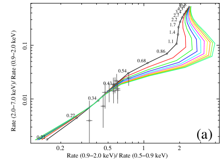
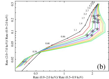
Figure 1: Hardness-hardness plot for an APEC thermal plasma, for two different representative Chandra ACIS-S3 observations. Each line corresponds to the locus of constant abundance (varying from 0.1 times Solar: black, to Solar: blue-green, in 0.1 increments) as kT varies (marked at various intervals). We assumed Solar abundance ratios (Asplund et al., 2004) and adopted redshifts of 0 (a) and 0.081 (b); all energy bands are in the observer’s frame. For illustration purposes, we show the measured hardness ratios in a series of different radial bins for two simulated observations, a and b, which are tailored to resemble the real systems of NGC 720 and RXJ 1159+5531 (Humphrey et al., 2011, 2012a). For both systems, the hardness ratios are sufficiently defined to constrain the temperature and, for object b, the abundance can be determined as well.

2.2 Required spectral resolution

Directly fitting a coronal plasma model to the full resolution spectrum of the hot gas provides the most reliable means for measuring the temperature and metallicity. Provided the abundance ratios of key species with respect to Fe are known (for example, if they match the Solar abundance pattern), however, hardness ratios (i.e. the ratio of the detected count-rates in two energy-bands) can also be used to extract temperature and abundance information.

For representative Chandra ACIS-S3 observations, we show in Fig 1 the loci in hardness-hardness space of APEC thermal plasma models having different temperatures and abundances. We have carefully chosen the energy-bands under scrutiny to maximize the separation of the models, but it is clear that two hardness ratios (i.e. three energy bands) are sufficient to constrain the gas temperature and abundance (and hence density) in these observations. Still, this approach requires careful calibration of the hardness ratios on an observation by observation basis, taking into account the spatial variation of the instrumental response, the Galactic absorbing column and the redshift of the source. For reference, we also show the corresponding hardness ratios in a series of radial bins for two simulated datasets (discussed in § 3.4), illustrating that, for real data, this provides a feasible means to measure the gas properties in multiple annuli.

2.3 Isothermal $\beta$-model

For an optically thin coronal plasma, we expect $\epsilon_{\nu^{\prime}}$ to depend only on the photon frequency ($\nu^{\prime}$), the gas density ($\rho_{g}$), temperature (expressed in energy units as kT), and abundances ($Z_{l}$) of key species (denoted here as $l$). As a simple illustration of the method, we therefore consider the case of such a plasma. Assuming spherical symmetry and isothermal gas with a $\beta$-model density profile,

$$\epsilon_{\nu^{\prime}}=n_{e,0}n_{H,0}\left(1+\frac{r^{2}}{r_{c}^{2}}\right)^{-3\beta}\sum_{l}4\pi\Lambda_{l}(kT)Z_{l}$$ (3)

where $n_{e,0}$ and $n_{H,0}$ are the central electron and Hydrogen number densities, respectively, $\Lambda_{l}$ relates the gas emissivity at frequency $\nu^{\prime}$ to the temperature for the species $l$, which has abundance $Z_{l}$. Here $r_{c}$ and $\beta$ are the standard parameters of the $\beta$-model (i.e. the “core radius” and $\beta$ parameter). In Appendix A, we derive a generalized expression for the surface brightness in terms of $\epsilon_{\nu^{\prime}}$. Substituting Eqn 3 into Eqn 22 and integrating, we obtain:

$$SB_{i_{0},i_{1}}^{k}\simeq F\sum_{j}N_{j}\sum_{i=i_{0}}^{i_{1}}\sum_{l}Z_{l}\int d\nu^{\prime}\overline{R}^{k}_{i}(\nu)\overline{P}_{\nu}^{j\rightarrow k}A_{eff}^{j\rightarrow k}\Lambda_{l}(kT)$$ (4)

where

$$F = \frac{n_{e,0}n_{H,0}}{(1+z)^{3}}\left(\frac{\Gamma(0.5)\Gamma(3\beta-0.5)}{\Gamma(3\beta)}\right)\frac{r_{c}^{3}}{D_{A}^{2}}$$ (5)

$$N_{j} = \left[\left(1+\frac{R_{j+1}^{2}}{r_{c}^{2}}\right)^{3\beta-\frac{3}{2}}-\left(1+\frac{R_{j}^{2}}{r_{c}^{2}}\right)^{3\beta-\frac{3}{2}}\right]$$ (6)

if $\beta\neq 0.5$. Here, $\Gamma$ is the gamma function. If $\beta=0.5$, then

$$N_{j} = \ln\left(\frac{r_{c}^{2}+R_{j+1}^{2}}{r_{c}^{2}+R_{j}^{2}}\right)$$ (7)

The integral in Eqn 4 does not depend on $\beta$ or $r_{c}$, and instead only depends on the (known) PHA bands used for surface photometry, the (known) annuli definitions and the (unknown) gas temperature. By fitting surface brightness profiles in multiple bands simultaneously, therefore, it is possible to constrain the temperature and abundance, along with $\beta$ and $r_{c}$. For speed it is often convenient to adopt a linear approximation for $\Lambda_{l}$; i.e.:

$$\Lambda_{l}(kT) \simeq \Lambda_{l}(kT_{m})\frac{T_{m+1}-T}{T_{m+1}-T_{m}}+\Lambda_{l}(kT_{m+1})\frac{T-T_{m}}{T_{m+1}-T_{m}}$$

where $m$ is chosen such that $kT_{m}\leq kT<kT_{m+1}$. (We note that this same approximation is used within the Xspec X-ray spectral fitting package for the computation of the APEC plasma emissivity.) This approximation means that kT can be taken outside of the integral in Eqn 4, allowing the integrals over $\nu^{\prime}$ to be pre-computed for speed.

2.3.1 Performance of the model

To illustrate the utility of this approach, we fitted the model to realistic, simulated Chandra surface brightness profiles. We assumed the hot gas was distributed as a $\beta$-model with $\beta=0.389$, $r_{c}=0.42$ kpc (which corresponds to 3.4″, adopting a distance of 25.7 Mpc) and a central gas density of $2.08\times 10^{-25}g\ cm^{-3}$. These parameters were chosen to be similar to the properties of the isolated, Milky Way-mass elliptical galaxy NGC 720 (Humphrey et al., 2011). Adopting 1 keV for the gas temperature and abundances which are 0.5 times Solar (Asplund et al., 2004), we simulated an artificial Chandra events file, using the algorithm outlined in Humphrey et al. (2013). Briefly, we computed the gas emissivity in a series of (R,z) bins in cylindrical polar coordinates, assuming an APEC thermal plasma model. Folding in the effective area and spectral response function of Chandra, we then simulated a corresponding spectrum from each region for a 100 ks exposure time, and the resulting photons were projected onto the sky to build up the event list. In Humphrey et al. (2013), we demonstrated the reliability of this method for producing artificial data. The resulting events file contains $\sim$20000 photons from the hot gas within a 4′ region. We added a background component with a constant surface brightness profile and a plausible spectrum (two soft APEC thermal plasma components, and a powerlaw, normalized to match the sky background in the vicinity of NGC 720). For simplicity, we ignored the spatial dependence of the effective area and spectral response, and ignored the spatial point spread of the telescope.

We extracted surface brightness profiles in three energy bands, 0.5–0.9 keV, 0.9–2.0 keV and 2.0–7.0 keV, corresponding to those shown in Fig 1. We fitted a model comprising the isothermal $\beta$-model described above (Eqn 4) for the hot gas and a constant background component in each band. We allowed $\beta$, $r_{c}$, the central gas density ($\rho_{g}$), kT and the gas abundance to be fitted freely. Fits were performed by minimizing the C-statistic, which is appropriate given the Poisson distributed nature of the data (e.g. Humphrey et al., 2009b; Cash, 1979) using dedicated software based around the MINUIT software library. By visual inspection, the overall fit was good and each parameter was recovered accurately, specifically within 2-$\sigma$ of the true value (kT=$0.99\pm 0.01$ keV, ${\rm Z_{Fe}}$=$0.43\pm 0.05$, $\beta=0.387\pm 0.003$, $r_{c}=0.40\pm 0.03$ kpc, and $\rho_{g}=(2.2\pm 0.2)\times 10^{-25}g\ cm^{-3}$). The ability to constrain both gas temperature and abundance by using these three energy bands is unsurprising given the temperature of the gas (Fig 1).

3 Mass analysis

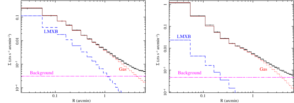
Figure 2: 0.9–2.0 keV surface brightness profiles for the simulated datasets a (left panel) and b (right panel). Overlaid (black solid lines) are the best-fitting entropy-based hydrostatic model, and the contribution to this model from hot gas (red dotted line), unresolved X-ray binaries (blue dashed line) and the background (magenta dash-dotted line). The overall fits are good.

We next consider a more physically motivated model for the surface brightness profile, based on a self-consistent solution to the equation of hydrostatic equilibrium for the density and temperature profiles.

3.1 Method

If the gas is spherically distributed and in an equilibrium state (although not necessarily static), we can write (Humphrey et al., 2008, 2013; Fang et al., 2009; Buote & Humphrey, 2012a):

$$\overline{r}^{2}\overline{S}^{\frac{3}{5}}\frac{d\overline{\zeta}}{d\overline{r}}=-\frac{2}{5}\left(\frac{GM_{500}}{r_{500}}\right)\left(\frac{\mu m_{H}}{kT_{ref}}\right)\left(\overline{M_{g}}+\overline{M_{ng}}-\overline{M_{eff}}\right)$$ (8)

$$\frac{\overline{S}^{\frac{3}{5}}}{\overline{r}^{2}}\frac{d\overline{M_{g}}}{d\overline{r}}=\left(\frac{4\pi r_{500}^{3}}{M_{500}}\right)\left(\frac{kT_{ref}}{\mu m_{H}S_{500}}\right)^{\frac{3}{2}}\overline{\zeta}^{\frac{3}{2}}$$ (9)

where $G$ is the Universal gravitational constant, $r_{500}$ is the radius within which the mean mass density of the system is 500 times the critical density of the Universe, $M_{500}$ is the mass within $r_{500}$, $\mu$ is the mean molecular weight ($\sim 0.62$ for a fully ionized plasma), $m_{H}$ is the mass of hydrogen, $kT_{ref}$ is an arbitrary reference energy (typically 1 keV), $\overline{r}$ is the radius from the centre of the object divided by $r_{500}$, $\overline{M}_{g}$ is the gas mass (divided by $M_{500}$) enclosed within radius $\overline{r}$, $\overline{M}_{ng}$ is the enclosed non-gas mass, $\overline{M}_{eff}$ is the “effective mass” codifying the bulk gas motions, including rotation (in the notation of Humphrey et al. 2013, $\overline{M}_{eff}=rv_{eff}^{2}/(GM_{500})$. For pure rotation, $v_{eff}$ is the spherically averaged rotation velocity at radius r). We define $\overline{S}=\rho_{g}^{-\frac{2}{3}}kT/(\mu m_{H}S_{500}(1-f_{nth}))$, corresponding to the usual astronomers’ entropy proxy, where $f_{nth}$ is the nonthermal pressure fraction (including the effects of magnetic pressure, cosmic ray pressure and turbulence), and

$$S_{500} = 150\left(\frac{M_{500}}{10^{14}M_{\odot}f_{b,U}E_{z}h_{70}^{2}}\right)^{\frac{2}{3}}\left(\frac{2+\mu}{5\mu}\right)^{\frac{2}{3}}\mu^{-1}m_{H}^{-\frac{5}{3}}$$

$$E_{z} = \Omega_{m}(1+z)^{3}+(1-\Omega_{m})$$ (10)

where $f_{b,U}$ is the Cosmological baryon fraction (0.17; Dunkley et al. 2009), $h_{70}$ is the Hubble constant in units of $70km\ s^{-1}Mpc^{-1}$, and $\Omega_{m}$ is the cosmological matter density parameter. We also define $\overline{\zeta}=\left(\rho_{g}kT/(\mu m_{H}(1-f_{nth})\right)^{\frac{2}{5}}\mu m_{H}S_{500}^{\frac{3}{5}}/kT_{ref}$, which is proportional to the thermal gas pressure to the power of $2/5$. The true values of $r_{500}$ and $M_{500}$ (which include the gas mass) are, technically, not known prior to solving the equations for $M_{g}$. However, since the scaling factors are arbitrary, we instead adopted the values of $r_{500}$ and $M_{500}$ appropriate for the dark matter halo alone, which can be computed analytically for a Navarro et al. (1997, hereafter NFW) profile.

By adopting parametrized models for $\overline{S}$, $\overline{M_{ng}}$, $f_{nth}$, and $\overline{M_{eff}}$, we can solve Eqns 8–9 numerically (e.g. with a fourth order Runge-Kutta method) for any given set of input parameters, and hence determine the radial density and temperature profiles. A reasonable model for $\overline{M}_{ng}$ comprises a stellar mass component (assuming mass follows light, this can be derived by deprojecting the stellar light; e.g. Binney et al. 1990; Cappellari et al. 2002; Humphrey et al. 2009a, 2012b) with adjustable M/L ratio, a central supermassive black hole, and a dark matter halo (e.g. NFW). If the gas is close to hydrostatic, $f_{nth}\simeq 0$ and $M_{eff}\simeq 0$, leaving it necessary only to adopt a parametrized form for $\overline{S}$, and provide two boundary conditions (on $\overline{M}_{g}$ and $\overline{\zeta}$).

We begin the integration from a small radius, $\overline{r}_{0}$, which is sufficiently small that we can impose the boundary condition $\overline{M}_{g}(<\overline{r}_{0})=0$, i.e. we assume there is no gas within $\overline{r}_{0}$. The boundary condition on $\overline{\zeta}$ is an adjustable parameter, which significantly affects the shape of the resulting gas temperature and density distribution. In particular, we found that the temperature profile shape can change from radially falling to radially rising (a “cool core” profile) by increasing $\overline{\zeta}(\overline{r}_{0})$. That changing the pressure boundary condition can produce such diverse behaviour is unsurprising (Mathews & Brighenti, 2003). The outer radius of integration is arbitrary, but it should be sufficiently large that it accounts for almost all of the emission that will be projected into the line-of-sight (see § A). We advocate some fraction (or multiple) of the virial radius as the optimal choice here, although it is important to understand that this requires that the gas remains approximately spherically distributed and hydrostatic (or, at least, accurately described by the adopted forms for $f_{nth}$ and $\overline{M}_{eff}$) out to this scale.

3.2 Simple entropy profile

In our recent work, we have assumed that the entropy depends on radius as a (multiply broken) powerlaw, plus a constant (see Humphrey et al. 2008, 2012a, 2013), i.e.

$$\overline{S} =s_{0}+s_{1}\overline{r}^{\alpha_{1}} (\overline{r}<\overline{r}_{b1})$$ (11)

$$=s_{0}+s_{1}\overline{r}_{b1}^{\alpha_{1}-\alpha_{2}}\overline{r}^{\alpha_{2}} (\overline{r}_{b1}\leq\overline{r}<\ldots)$$

and so on, adding in as many breaks as required. The parameters $s_{0}$, $s_{1}$, $\alpha_{1}$, $\alpha_{2}$ and $r_{b1}$ are adjustable. Empirically, observed entropy profiles are often well parametrized by similar models (e.g. Mahdavi et al., 2005; Donahue et al., 2006; Jetha et al., 2007; Finoguenov et al., 2007; Gastaldello et al., 2007a; Sun et al., 2009; Cavagnolo et al., 2009; Johnson et al., 2009; Pratt et al., 2010; Humphrey et al., 2012a; Werner et al., 2012). Theoretically, powerlaw-like entropy profiles are expected from adiabatic structure formation models (Tozzi & Norman, 2001; Voit et al., 2005), which may be modified by feedback, resulting in profiles that resembles (multiply) broken powerlaw distributions, with a constant offset (e.g. Voit & Donahue, 2005; McCarthy et al., 2010).

3.3 Metallicity profile

In order to convert the measured gas density and temperature into a surface brightness profile, it is necessary to know the three dimensional radial dependence of the abundance pattern. In practice, one can adopt a simple parametrization, the free parameters of which can be fitted along with the parameters controlling the mass model and thermodynamic properties of the gas. Unfortunately there is no generally accepted functional form for such a distribution, and so we recommend experimentation with different metallicity profiles as a means of exploring the sensitivity of the results to the details of this assumption. For the purpose of validating the surface brightness model as an adequate tool for fitting, it is convenient to adopt flat (i.e. constant) metallicity profiles in this paper. We allowed only the total (Fe) abundance to be fitted, while fixing the abundance ratios of other metals with respect to Fe to be at their Solar values (Asplund et al., 2004). We return to the problem of a radially varying abundance profile in § 5.3.

3.4 Performance of the model

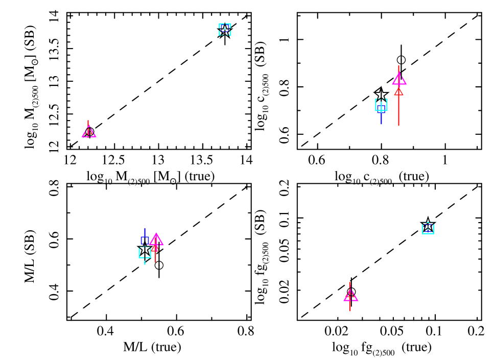
Figure 3: Accuracy of various physical parameters obtained from narrow-band photometric fits. We compare total mass (M), halo concentration (c), stellar mass-to-light ratio (M/L) and gas fraction ($f_{g}$) measurements. For simulated 100 ks datasets a (triangles) and b (squares), the parameters derived from fitting the hydrostatic model with a “simple entropy profile” (small symbols) and the ScAM model (large symbols) are shown on the y-axes, and the true value is shown as the x-axis. The dashed lines indicate equality ($y=x$). Comparisons are made between parameters at either ${\rm R_{2500}}$ (for NGC 720) or ${\rm R_{500}}$ (for RXJ 1159+5531), indicated by the 2(500) notation. We find that the model fit results are both precise and accurate, being within $\sim 2\sigma$ of the true value in each case. As expected, the constraints obtained with the ScAM model are tighter. In addition, we also show the results of fitting the ScAM model to a 5 ks snapshot observation of object a (large circles), demonstrating the utility of this model with shallow exposures. For clarity, these points are shown slightly displaced in the x-direction. We show (large stars) the results of fitting the ScAM model to object b, but allowing the Fe abundance profile to peak in the centre (see § 5.3).

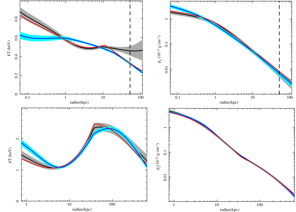
Figure 4: Three dimensional temperature and density profiles for simulated objects a (top panels) and b (lower panels), obtained from fitting the hydrostatic narrow band photometric model with a simple entropy profile (grey region) and the ScAM model (blue region) to the 100 ks simulated datasets. The red line shows the true profile. The shaded regions indicate 1-$\sigma$ confidence regions. The dashed vertical line in the upper panels corresponds to $\sim$7′, demarcating the region for which surface brightness fits were performed. In these panels, the radial scale spans 0.5″–15′, which is close to ${\rm R_{2500}}$. In the lower panels, the radial range corresponds to $\sim$0.5″–7′, which is close to ${\rm R_{500}}$. The simple entropy fits generally do a good job at recovering the true profiles, although at the largest scales in object a, the temperature is slightly over-estimated. This most likely reflects partial degeneracy with the background. Given its more restrictive assumptions, the ScAM model does a poorer job at recovering the true temperature and density profiles, especially in the centres of each system. Nevertheless, the average properties of the gas, in particular at large scales, are recovered reasonably well, which explains why the global properties of the systems are measured accurately (Fig 3).

To illustrate the performance of the model, we fitted simulated Chandra data for two objects, spanning almost two orders of magnitude in mass. These objects, henceforth termed objects a and b, are tailored to resemble, respectively, the isolated, Milky Way-mass elliptical galaxy NGC 720 and the fossil group/ cluster RXJ 1159+5531 (Humphrey et al., 2011, 2012a). These systems were chosen as we have previously studied them over a wide range of physical scales using the more traditional approach of spatially resolved spectroscopy. Starting with the published models for each real system, and assuming ${\rm Z_{Fe}}$=0.5 times Solar, we simulated artificial events files corresponding to a 100 ks exposure with Chandra ACIS-S3. These files were generated as described in § 2.3.1 (see also Humphrey et al., 2013). To represent better real data, we included an additional component to represent the unresolved X-ray binary contribution to each system. Specifically, we assumed the combined light from the LMXBs was distributed as de Vaucouleurs profiles, with effective radii 25.2″ and 6.4″, respectively, and a 7.3 keV bremsstrahlung spectrum. We added a background component with a constant surface brightness profile and a plausible spectrum (two soft APEC thermal plasma components, and a powerlaw, normalized to match the sky background in the vicinity of NGC 720). This is somewhat idealized as it omits the non X-ray background that is important for Chandra data at high energies. For simplicity, we also ignored the spatial dependence of the effective area and spectral response, and ignored the spatial point spread of the telescope.

We extracted surface brightness profiles in three energy bands, 0.5–0.9 keV, 0.9–2.0 keV and 2.0–7.0 keV, corresponding to those shown in Fig 1, which were fitted simultaneously. The model comprised hot gas, a background component and a deVaucouleurs component to model the unresolved point sources. The hot gas model was derived by numerically solving Eqns 8–9, assuming $\overline{M_{eff}}\equiv 0$ and $f_{nth}=0$ (i.e. no nonthermal pressure), and modelling $\overline{M_{ng}}$ as the sum of a stellar light model (as discussed in Humphrey et al., 2011, 2012a), an NFW dark matter halo and a central black hole. The stellar M/L ratio and the mass and concentration of the NFW model were allowed to vary in the fit, and the black hole mass was fixed at $3\times 10^{8}$${\rm M_{\odot}}$ for NGC 720 and $2.4\times 10^{9}$${\rm M_{\odot}}$ for RXJ 1159+5531. The model assumed a flat abundance profile, but we allowed the overall abundance to fit freely, fixing the abundance ratios with respect to Fe to their Solar values.

To compute the surface brightness, we evaluated the gas emissivity at a series of logarithmically spaced radial points (from $\overline{r}_{0}$ to 1–2 times the virial radius), and projected it using a cubic spline approximation and Eqn 28. To enable direct comparison with our previous work, parameter space exploration was carried out with a Bayesian Monte Carlo code (version 2.7 of the MultiNest code: Feroz et al., 2009). We adopted the appropriate Poisson likelihood function for a set of independent data points, and used uniform priors for all variable parameters, similar to our default analysis in Humphrey et al. (2011, 2012a).

The model gave a good fit to both datasets (see Fig 2), and the abundance was measured reasonably well for each system (${\rm Z_{Fe}}$=$0.58\pm 0.18$, $0.40\pm 0.06$) In Fig 3, we compare various derived physical parameters obtained from our fits to the known, true value, demonstrating good overall agreement, and indicating that the hydrostatic, narrow band photometric model provides a viable means for constraining the global properties of elliptical galaxies, groups and clusters. The constraints are comparable to those obtained from our fits to the full spatially resolved spectroscopic data of NGC 720 and RXJ 1159+5531 (Humphrey et al., 2011, 2012a); for example we measured ${\rm M_{500}}$ and ${\rm c_{500}}$ in RXJ 1159+5531 to 0.05 dex and 6%, respectively, with both the surface brightness fitting approach and the full spectral analysis, if restricted only to the Chandra data (Humphrey et al., 2012a). In Fig 4, we show the derived temperature and density profiles for each object, which agree well with the true profile. For object a, the temperature at large scales is slightly over-estimated, albeit with large uncertainty. At these scales, the background is comparable to, or exceeds, the hot gas flux, at least at energies $\mathrel{\hbox to0.0pt{\lower 3.0pt\hbox{$\sim$}\hss}\raise 2.0pt\hbox{$>$}}$ 1 keV, which limits the ability to constrain the temperature precisely from the hardness ratios. Nevertheless, the global properties of the system are very well recovered. This illustrates the potential of narrow band photometry for mass measurements over a range of mass scales.

4 The Scaled Adiabatic Model (ScAM)

While Eqn 11 is appealing in its simplicity and has been used successfully to model the X-ray emission from galaxies and groups (e.g. Humphrey et al., 2008, 2009a, 2011, 2012a, 2012b), it has significant drawbacks. In particular, extrapolating the model to large radii involves ad hoc assumptions in a region where the data are often sparse, at best, or missing altogether. Furthermore, as the entropy profile shape becomes more and more complex, additional adjustable parameters are required, resulting in a large number of potentially degenerate parameters. These problems are amplified if the S/N of the data is low.

Instead, we propose here to employ an alternative parametrization for the entropy distribution. Outside the very central regions, gravity-only models of structure formation predict a “baseline” distribution, $\overline{S}\simeq\overline{r}^{1.1}$ (Voit et al., 2005), which is distorted by non-gravitational heating, especially in the inner parts of low-mass systems (e.g. Sanderson et al., 2003; Cavagnolo et al., 2009; Pratt et al., 2010). Nevertheless, the principal effect of the entropy injection is to lower the gas density, rather than raise the temperature (e.g. Ponman et al., 1999; Pratt et al., 2010; Mathews & Guo, 2011), which is supported by the universality of cluster and group temperature profiles (e.g. Vikhlinin et al., 2005; Gastaldello et al., 2007b). Thus, to zeroth order, $\overline{S}\simeq\overline{r}^{1.1}\left(f_{g}/f_{b,U}\right)^{-\frac{2}{3}}$, where $f_{g}$ is the gas fraction. This scaling has been found to give a much better match to the observed entropy profiles than the baseline model when the enclosed gas fraction, $f_{g}=\overline{M_{g}}/(\overline{M_{g}}+\overline{M_{ng}})$ is employed (Pratt et al., 2010; Humphrey et al., 2011, 2012a, 2012b). As we show below, this model fails to match the data successfully in lower mass objects, and in the central parts of all systems (roughly, within the cooling radius). We therefore begin by refining the parametrization of this scaling relation.

4.1 Calibrating the model

Object	z	${\rm R_{500}}$	$R_{max}$	$K_{500}$	Dataset	Exposure	ref
		(kpc)	(kpc)	($keV\ cm^{2}$)		ks
NGC 4125	0.004523	$166\pm 18$	47	$20\pm 4$	2071(C)	63	1
NGC 720	0.005821	$199\pm 9$	74	$28\pm 3$	7062, 7372, 8448, 8449 (C)	99	2
					800009010 (S)	177	2
NGC 6482	0.013129	$205\pm 17$	97	$32\pm 5$	3218(C)	17	3
NGC 4261	0.007465	$447\pm 45$	190	$142\pm 27$	834, 9569(C)	135	4
MKW4	0.02	$511\pm 24$	130	$182\pm 17$	3234(C)	30	1
RXJ 1159+5531	0.081	$577\pm 17$	1200	$232\pm 14$	4964(C)	75	5
					804051010(S)	85	5
A 1991	0.0587	$718\pm 14$	680	$336\pm 13$	3193(C)	38	6
A 2589	0.0414	$997\pm 58$	720	$645\pm 77$	7190(C)	53	6
A 133	0.0566	$1150\pm 25$	710	$858\pm 26$	9897(C)	69	6
A 907	0.1527	$1180\pm 30$	1400	$966\pm 51$	3205(C)	41	6
A 1413	0.1427	$1290\pm 20$	1990	$1140\pm 40$	5003(C)	75	6

Table 1: Data used for calibrating the scaled adiabatic model. For each target, we list the name, redshift (z), ${\rm R_{500}}$ derived from our own fits to the data, the maximum radius to which the data were fitted ($R_{max}$), the characteristic entropy ($K_{500}$) derived from our fits, the dataset observation identifier for both the Chandra (C) or Suzaku (S) data, the cleaned exposure time and a reference to the literature describing the data reduction and analysis. References: (1) Humphrey & Buote (2010); (2) Humphrey et al. (2011); (3) Humphrey et al. (2006); (4) Humphrey et al. (2009a); (5) Humphrey et al. (2012a); (6) W. Liu et al, in preparation.

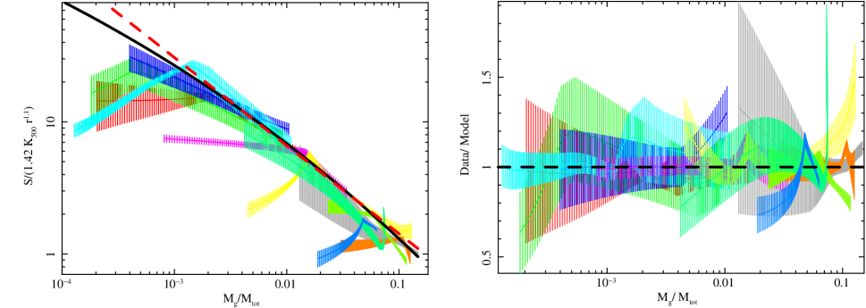
Figure 5: Relation between the scaled entropy and the gas fraction for the sample of galaxies, groups and clusters (left panel). The shaded regions correspond to 1-$\sigma$ confidence intervals. The solid black line is the best-fitting simultaneous model fit to the data excluding the cool cores of each system (Eqn 12–13) , which are generally apparent as a positive correlation between the enclosed gas fraction and the scaled entropy. The dashed red line is the expectation if the scaling adopted by Pratt et al. (2010) is exact. In the right panel, we show the ratio between the observed profiles and the ScAM parametrization of the entropy–${\rm f_{g}}$ relation (§ 4; Eqn 12–14). While not exact in any given system, we find that ScAM captures the overall shape of the entropy distribution over a wide range of gas fractions (hence, wide radial range), including in the cool cores.

To calibrate the relation between the gas entropy and the gas fraction, we assembled a sample of relaxed, X-ray luminous galaxies, groups and clusters with good quality Chandra data to a significant fraction of ${\rm R_{500}}$ (Table 1). The Chandra data were reduced and analyzed to provide projected temperature and density profiles (deprojected for NGC 4125 and MKW4), as described in Humphrey & Buote (2010); Humphrey et al. (2011, 2012a); Liu et al. (2012b). For NGC 720 and RXJ 1159+5531, we used both the Chandra and Suzaku data described in Humphrey et al. (2011, 2012a). Using the approach outlined in § 3, we solved Eqn 8–9 to obtain self-consistent models for the deprojected temperature and density profiles, given parametrized input models for the gravitating mass and entropy (for which we used a multiply broken powerlaw, i.e. Eqn 11). These models were projected along the line of sight, as needed, following the procedure described in Humphrey et al. (2011), and fitted to the observed data.

While this approach limits the flexibility of the inferred entropy profiles by imposing a parametric form, it has the advantage of providing complementary entropy, mass and gas fraction profiles. Furthermore, models of this form have previously been shown to provide an adequate fit to galaxies, groups and clusters. In Fig 5, we show the scaled entropy as a function of enclosed gas fraction. The data are shown for each system, starting at the smallest resolvable scales and extending to $\sim$${\rm R_{500}}$. At large ${\rm f_{g}}$ values, the scaled entropy profiles show little scatter, indicating scaling similar to that pointed out by Pratt et al. (2010). However, we note that the Pratt et al. (2010) scaling does not exactly describe the relationship, as it deviates at smaller values of ${\rm f_{g}}$. At the smallest ${\rm f_{g}}$ values, approximately corresponding to the cooling core, the relationship becomes non-monotonic, and exhibits significant scatter from system to system.

To parametrize the relationship, we begin by assuming a relation of the form:

$$\overline{S}=s_{0}+(1-s_{0})\overline{r}^{1.1}\overline{S}^{\prime}\left(\frac{f_{g}}{f_{b,U}}\right)$$ (12)

where $s_{0}$ is a central entropy value, and $\overline{S}^{\prime}$ is an empirical scaling function that is chosen to fit observations. With experimentation, we found that we were able to fit the data satisfactorily (Fig 5, right panel) by employing a model of the form:

$$\overline{S}^{\prime} = s_{n}\exp\left(-s_{e}\left(\frac{f_{g}}{f_{b,U}}\right)^{s_{i}}\right)$$ (13)

if $f_{g}\geq f_{g1}$, or

$$\overline{S}^{\prime} = s_{n}\exp\left(-s_{e}\left(\frac{f_{g1}}{f_{b,U}}\right)^{s_{i}}\right)\left(\frac{f_{g}}{f_{g1}}\right)^{-s_{a}}$$ (14)

otherwise, where $s_{n}$, $s_{e}$, $s_{i}$, $f_{g1}$, $s_{0}$ and $s_{a}$ are adjustable parameters. In practice, we found that $s_{n}=3440$, $s_{e}=10.6$ and $s_{i}=0.076$ gave a good description of the data in most cases. The remaining parameters, which all relate to the distribution of the entropy within the core of the system, need to be adjusted from object to object.

4.2 Performance of the model

Parameter	Recommended value
$\log_{10}$ ${\rm M_{500}}$	free parameter
$\log_{10}$ ${\rm c_{500}}$	free parameter
M/L∗	free parameter
$M_{BH}$	free parameter (where possible)
$s_{0}$	free parameter
$s_{a}$	free parameter
$f_{g1}$	free parameter
$s_{n}$	3440
$s_{e}$	10.6
$s_{i}$	0.076
$\overline{\zeta}$	free parameter
${\rm Z_{Fe}}$	free parameter

Table 2: Summary of variable and fixed parameters for the ScAM model.

Having eliminated $\overline{S}$ by application of Eqn 12–14, we solved Eqn 8–9 and computed surface brightness profiles, which we fitted to the data for NGC 720 and RXJ 1159+5531, exactly as described in § 3.4. In Table 2 we summarize the fitted and fixed parameters. In Fig 3 we compare the derived properties for the simulated objects a and b with the true values, finding overall excellent agreement. The gas abundance was measured accurately (${\rm Z_{Fe}}$=$0.58\pm 0.18$ and $0.59\pm 0.06$, respectively) In Fig 4, we show the derived temperature and density profiles for both systems. Overall, the fits are reasonable, but in the inner regions, we see statistically significant (albeit not dramatic) deviations of the best fitting model from the true profiles. Nevertheless, at large scales the ScAM model does a good job of capturing the shapes of the profiles, explaining why the global parameters are so well recovered. These results give us confidence in the utility of the Scaled Adiabatic Model (ScAM) to derive global physical parameters from narrow-band photometry.

Since the ScAM model imposes restrictions on the entropy profile distribution at large scales, it is ideally suited for fitting low-to-modest S/N data. To demonstrate its usefulness, we simulated data corresponding to a 5 ks snapshot of object a, corresponding to only 5% of the exposure used in our previous discussion. Fitting the surface brightness profiles, we found that the global parameters were accurately recovered. While the precision of the constraints was poorer than when fitting the same model to the 100 ks exposure, the global parameters were, nevertheless, recovered to within $\sim$0.1 dex or better.

5 Discussion

5.1 Narrow band photometry as a practical tool

We have demonstrated that narrow band photometry provides an effective alternative to spatially resolved spectroscopy for determining detailed mass profiles of X-ray luminous galaxies, groups and clusters. Since surface photometry is, in general, less demanding of data than spectroscopy, the narrow band photometric method presented here is ideally suited to systems with modest S/N, for which spatially resolved spectroscopy is not realistic. Without the intermediate step of measuring temperature and density profiles (from single phase plasma model fits), biases due to the projection of different temperature gas components along the line of sight are effectively minimized, and the difficulty of accounting for covariance between the temperature and density data points downstream is circumvented.

In our fully Bayesian forward-fitting analysis, a model for the surface brightness profile in each band is constructed based on a physical model for the mass distribution and the entropy profile, assuming hydrostatic equilibrium, a single phase gas and spherical symmetry, and is directly fitted to the data. Although real galaxy clusters are not exactly spherical, on average the spherical approximation does not introduce significant bias into their inferred global properties, such as the virial mass, halo concentration, and gas fraction (Buote & Humphrey, 2012c). Similarly, the hydrostatic approximation, provided the system is sufficiently relaxed in its X-ray morphology, is likely to be accurate at least to the $\sim$25% level (Buote & Humphrey, 2012a, and references therein). In regions where the gas is morphologically relaxed, spatially resolved spectroscopy is generally consistent with a single phase plasma, provided the temperature gradient is not strong across the aperture (e.g. Molendi & Pizzolato, 2001; Lewis et al., 2002; Humphrey & Buote, 2006). Similarly, the range of temperatures in the cores of clusters measured within the XMM RGS aperture (Peterson et al., 2003) is broadly consistent with the observed central temperature gradients. Limited multiphase gas has, nevertheless, been inferred in regions of strong interaction between the hot gas and ejecta from a central AGN (e.g. Molendi, 2002; Buote et al., 2003a; David et al., 2011). Recent work has also invoked multiphase gas as a possible explanation of the unexpected flattening of cluster entropy profiles outside $\sim$${\rm R_{500}}$ (Simionescu et al., 2011; Urban et al., 2011), although observations of relaxed clusters suggest such behaviour (and, hence, the postulated clumping) is not ubiquitous (Humphrey et al., 2012a; Miller et al., 2012; Eckert et al., 2012).

While it is relatively straightforward to identify and exclude data from the disturbed cores of clusters (where the hydrostatic and single phase approximations may break down), the effects of possible clumping at large scales are more troubling, due to projection effects. Still, if one focuses on regions well within projected ${\rm R_{500}}$, the projected emission from outside ${\rm R_{500}}$ is unlikely to contribute significantly along the line of sight, in which case the results should not depend sensitively on the behaviour of the entropy in the outskirts of the cluster. This can be tested explicitly by varying the maximum radius used during the projection calculation. Application of the photometry method to the outskirts of clusters can, of course, also be used to test the need for clumping or deviations from hydrostatic equilibrium in those regions. If necessary, given a physical model for the clumping, the expression for $\epsilon_{\nu^{\prime}}$ can be modified to compensate and allow a useful measurement of the gravitating mass even in those regions.

While the number of energy bands used is entirely arbitrary, we found that three standard bands (0.5–0.9 keV, 0.9–2.0 keV and 2.0–7.0 keV) were sufficient to constrain the gas temperature and total abundance from Chandra data over a fairly wide range of parameter space. Limiting the number of photometric bands is desirable, since it minimizes the number of adjustable parameters needed to account for the background. Nevertheless, if the data permit, the number of energy bands can be expanded to focus on regions of particular interest that may help constrain the relative abundance of other species, such as O, Ne, Mg and Si.

5.2 The entropy parametrization

We present two classes of hydrostatic model that enable the gravitating mass to be inferred. Both involve a physical model for the (non-gas) gravitating mass (comprising dark matter halo, stars and central black hole), and solving the hydrostatic equations (Eqn 8–9) by imposing a constraint on the entropy distribution. The performance of the former approach, which entails adopting an arbitrary parametrization for the entropy profile, has been demonstrated in our previous, spatially resolved spectrocopic fits to X-ray data (Humphrey et al., 2008, 2009a, 2011, 2012a, 2012b), and, independently, in fits to Sunyaev-Zeldovich data (Allison et al., 2011). Combined with narrow-band photometry, we have demonstrated that precise, accurate constraints can be obtained on the global properties of objects over a wide mass range.

The latter entropy parametrization is more suitable for lower S/N data, since it involves exploiting an empirical scaling relation between the gas fraction and entropy profile outside the cooling core, effectively eliminating the arbitrariness in the extrapolation of the entropy profile to large scales. This scaling relation is unlikely to be exact in any given system, which introduces systematic errors into the recovered temperature and density profiles, especially in the system cores. However, with the extra constraints at large scale, we found that the reduction in the error-space did not give rise to appreciable biases in the derived global system properties. The utility of this method is illustrated by the fact that, even for a shallow, snapshot observation of a realistic low-mass object, we were still able to recover the global parameters to within $\sim$0.1 dex.

5.3 Abundance gradients

For simplicity, our simulations were for systems with a constant metallicity profile. In reality morphologically relaxed systems tend to have centrally-peaked metallicity distributions (e.g. De Grandi & Molendi, 2001; Buote et al., 2003b; Humphrey & Buote, 2006; Johnson et al., 2011) and so, if the properties in the centre of the system are important it is necessary to modify the model to incorporate such a gradient. As there is no de facto standard model for such purposes, we recommend a simple ansatz, such as:

$$Z_{Fe}=Z_{Fe,1}+\left(Z_{Fe,0}-Z_{Fe,1}\right)\left(1+\frac{r^{2}}{r^{2}_{Fe}}\right)^{-\alpha_{Fe}}$$ (15)

where $Z_{Fe,0}$ and $Z_{Fe,1}$, $r_{Fe}$ and $\alpha_{Fe}$ are adjustable fit parameters, and we initially assume that the ratio of the abundance of the other metals to Fe does not vary with radius. To verify that adopting such a parametrization does not appreciably degrade the constraints on the global system parameters, we re-simulated object b, assuming Eqn 15. We set $log_{10}Z_{Fe,0}=0.0$, $log_{10}Z_{Fe,1}=-0.5$, $log_{10}r_{Fe}=1.0$ [kpc] and $\alpha_{Fe}=0.5$. We fitted the surface brightness profiles, using the ScAM model (this time incorporating Eqn 15) and allowing the parameters $Z_{Fe,0}$, $r_{Fe}$ and $\alpha_{Fe}$ to be fitted. We summarize the constraints on the global parameters in Fig 3, demonstrating that incorporating an abundance gradient into our fits does not significantly degrade the level of constraints we can obtain. Furthermore, with this approach, we were also able to constrain the abundance profile reliably (we measured $log_{10}Z_{Fe,0}=0.06\pm 0.09$, $log_{10}r_{Fe}=0.97^{+0.20}_{-0.15}$ [kpc] and $\alpha_{Fe}=1.14^{+0.26}_{-0.40}$).

5.4 The Sunyaev-Zeldovich effect

While we have focused on the use of the ScAM model in the context of narrow-band X-ray photometry, it actually has broader implications. In particular, it is a potentially powerful tool for constraining the global properties of galaxy clusters from the Sunyaev-Zeldovich (S-Z) effect (Birkinshaw, 1999, for a review). The key observable is the Compton y-parameter,

$$y=\frac{\sigma_{T}}{m_{e}c^{2}}\int_{los}n_{e}kTdl$$ (16)

where $\sigma_{T}$ is the Thompson scattering cross-section, $m_{e}$ is the mass of the electron, $c$ is the speed of light, $n_{e}$ is the electron number density, and the integral is along the line-of-sight (los). In comparison to X-ray emission, for which the emissivity depends on the density squared, the y-parameter is more sensitive to the properties of the gas at large radii.

In order to derive the physical properties of a system from the inferred y-parameter, it is necessary to construct a model for the spatial variation in both density and temperature. Models employing ad hoc parametrization for the thermodynamical state of the gas, for example the isothermal $\beta$-model, or even the simple entropy-based model discussed in § 3 (for the application of this kind of model to S-Z data, see Allison et al., 2011), cannot be guaranteed to capture the true behaviour of the gas when extrapolated to large scales. On the other hand, the thermodynamic behaviour of the gas at large radii predicted by the ScAM model is determined entirely by the underlying scaling relation, and it is clear from Fig 4 that it is sufficiently accurate to model morphologically relaxed objects with very different mass distributions, density and temperature profiles. While it remains to be seen whether there exist clusters for which the empirical ScAM scaling does not (at least approximately) hold, the well-determined asymptotic behaviour of the model is very desirable in S-Z studies, and so we strongly advocate its use.

Appendix A Computing the X-ray Surface Brightness Profile

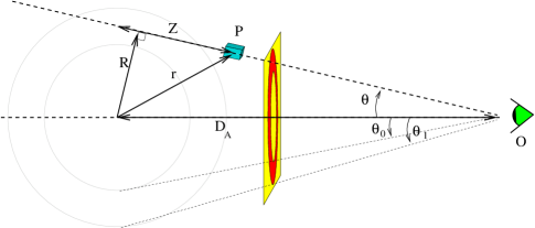
Figure 6: Schematic view showing the projection of the object onto the plane of the sky (shown schematically in yellow). The gas properties at point P are a function only of the radial distance from the centre of the object (r), while the distance to the observer (O) is $D_{A}$. The distance along the line of sight to the parcel is denoted as $Z$, and the inner and outer radii of an arbitrary shell of gas (shown in red) correspond to incidence angles $\theta_{0}$ and $\theta_{1}$, respectively.

In this section, we discuss the efficient computation of the X-ray surface brightness model, which is critical for making narrow-band photometry a useful tool for model fitting.

A.1 The Surface Brightness Distribution

Consider a small parcel of gas of volume dV, which is emitting a total (rest frame) photon flux (i.e. photons s^-1) of $\epsilon_{\nu^{\prime}}dVd\nu^{\prime}$ at frequency $\nu^{\prime}$. Let the system be spherically symmetric (see Fig 6), so that $\epsilon_{\nu^{\prime}}$ is a function of distance, r, from the centre of the system. The total photon flux incident on a telescope aperture of area A placed at angular size distance $D_{A}$ from the gas parcel will be:

$$N_{\nu}d\nu=\frac{A\epsilon_{\nu^{\prime}}(r)dVd\nu^{\prime}}{4\pi D_{A}^{2}(1+z)^{3}}=\frac{A\epsilon_{\nu^{\prime}}(r)d\Omega dZd\nu^{\prime}}{4\pi(1+z)^{3}}$$ (17)

where $z$ is the observed redshift of the gas parcel, $\nu=\nu^{\prime}(1+z)^{-1}$ is the observed photon frequency, $d\Omega$ is the angular size subtended by the gas parcel at the telescope, and $Z$ is the line of sight coordinate in the rest frame of the gas parcel, so that $r=r(\theta,Z)$.

The arriving photons pass through the telescope optics and are (possibly) detected in a focal plane detector. The detected photon flux at position (x,y) in “pulse height channel” (i.e. energy bin) $i$ is given by:

$$dC_{i}(x,y)=N_{\nu}d\nu\ P_{\nu}(x,y,\theta,\phi)E_{\nu}(x,y,\theta,\phi)\mathbb{R}_{i}(x,y,\nu)$$ (18)

where $P_{\nu}(x,y,\theta,\phi)$ codifies the telescope spatial point spread function at frequency $\nu$ for photons arriving with incident angle $\theta$ and azimuthal angle $\phi$ (i.e. it represents the likelihood that such a photon would be detected at position (x,y)), $E_{\nu}$ is the combined detection efficiency of the optics and detector, and $\mathbb{R}_{i}$ codifies the spectral redistribution function, i.e. indicating the likelihood that a photon with frequency $\nu$ that is detected at position (x,y) will be assigned to pulse height channel i.

To make further progress, we divide the sky into a series of concentric annuli, the centres of which coincide with the projected centre of the object. Annulus $j$ has inner and outer radii $\theta_{j}$ and $\theta_{j+1}$, respectively. Now, let us compute the total counts $C_{i}^{k}$ detected in pulse height channel $i$ within some (arbitrary) region of the detector, defined by the function $\delta_{k}(x,y)$, which is 1 in the region, or 0 elsewhere. It follows that:

$$C_{i}^{k}=\int\delta_{k}(x,y)dx\ dy\ \sum_{j}\int_{0}^{2\pi}d\phi\int_{\theta_{j}}^{\theta_{j+1}}\sin\theta d\theta\ \int_{-\infty}^{\infty}dZ\bigg{[}$$

$$\int d\nu^{\prime}\frac{A\epsilon_{\nu^{\prime}}(r)}{4\pi(1+z)^{3}}P_{\nu}(x,y,\theta,\phi)E_{\nu}(x,y,\theta,\phi)\mathbb{R}_{i}(x,y,\nu)\bigg{]}$$ (19)

where x and y are coordinates on the detector. Now, let annulus $j$ be sufficiently narrow that $P_{\nu}(x,y,\theta,\phi)\simeq P_{\nu}(x,y,\theta_{j},\phi)$ and $E_{\nu}(x,y,\theta,\phi)\simeq E_{\nu}(x,y,\theta_{j},\phi)$, so that we can rewrite

$$C_{i}^{k}\simeq\sum_{j}\int d\nu^{\prime}\bigg{[}\int\delta_{k}(x,y)dx\ dy\ \mathbb{R}_{i}(x,y,\nu)$$

$$\int_{0}^{2\pi}d\phi P_{\nu}(x,y,\theta_{j},\phi)A\ E_{\nu}(x,y,\theta_{j},\phi)\bigg{]}$$

$$\times\bigg{[}\int_{\theta_{j}}^{\theta_{j+1}}\sin\theta d\theta\int_{-\infty}^{\infty}\frac{\epsilon_{\nu^{\prime}}(r)}{4\pi(1+z)^{3}}dZ\bigg{]}$$ (20)

It is convenient to rewrite this as:

$$C_{i}^{k} \simeq \sum_{j}\int d\nu^{\prime}\bigg{[}\overline{\mathbb{R}}^{k}_{i}(\nu)\overline{P}_{\nu}^{j\rightarrow k}A_{eff}^{j\rightarrow k}\bigg{]}\times\bigg{[}n_{\nu}^{j}\bigg{]}$$ (21)

where the quantity $R^{k}_{i}(\nu)$ is the spectral redistribution function, $P_{\nu}^{j\rightarrow k}$ is the spatial “point response function” linking sky annulus $j$ to detector region $k$, $A_{eff}^{j\rightarrow k}$ is the “effective area” linking annulus $j$ to detector region $k$, and

$$n_{\nu}^{j}=\int_{\theta_{j}}^{\theta_{j+1}}\sin\theta d\theta\int_{-\infty}^{\infty}\frac{\epsilon_{\nu^{\prime}}(r)}{4\pi(1+z)^{3}}dZ$$ (22)

$$=\int_{\theta_{j}}^{\theta_{j+1}}\sin\theta d\theta\int_{D_{A}\sin\theta}^{\infty}\frac{2}{(1+z)^{3}}\frac{r(\epsilon_{\nu^{\prime}}/4\pi)dr}{\sqrt{r^{2}-D_{A}^{2}\sin^{2}\theta}}$$ (23)

Changing the order of integration, this becomes:

$$n^{j}_{\nu} = \frac{2}{(1+z)^{3}}\int_{R_{j}}^{\infty}\frac{\epsilon_{\nu^{\prime}}}{4\pi}r\ dr\int_{\theta_{j}}^{\Theta_{j+1}}\frac{\sin\theta d\theta}{\sqrt{r^{2}-D_{A}^{2}\sin^{2}\theta}}$$ (24)

$$\equiv \frac{2}{(1+z)^{3}}\int_{R_{j}}^{\infty}\frac{\epsilon_{\nu^{\prime}}}{4\pi}r\ I_{j}(r)dr$$ (25)

where $\Theta_{j+1}={\rm min}\left({\rm asin}(r/D_{A}),\theta_{j+1}\right)$ is introduced due to the change of the order of integration and the requirement that $r>D_{A}sin\theta$, and $R_{j}=D_{A}\sin\theta_{j}$, and $I_{j}(r)=\int_{\theta_{j}}^{\Theta_{j+1}}\sin\theta d\theta/\sqrt{r^{2}-D_{A}^{2}\sin^{2}\theta}\simeq\left(\sqrt{r^{2}-D_{A}^{2}\theta_{j}^{2}}-\sqrt{r^{2}-D_{A}^{2}\Theta_{j+1}^{2}}\right)/D_{A}^{2}$, applying the small angle approximation $\sin\theta\simeq\theta$ and integrating.

Now, let us define the X-ray surface brightness in a particular PHA channel band ($i_{0}$–$i_{1}$),

$$SB^{k}_{i_{0},i_{1}} = \frac{\sum_{i=i_{0}}^{i_{1}}C_{i}^{k}}{A_{k}}=\frac{\sum_{j}\int d\nu^{\prime}\overline{P}_{\nu}^{j\rightarrow k}A_{eff}^{j\rightarrow k}n_{\nu}^{j}\sum_{i=i_{0}}^{i_{1}}\overline{\mathbb{R}}_{i}^{k}}{A_{k}}$$

where $A_{k}\equiv\int\delta_{k}(x,y)dx\ dy$ is the area of detector region $k$. Provided the PHA channel range $i_{0}$–$i_{1}$ is sufficiently narrow, and the redistribution function $\overline{\mathbb{R}}^{k}_{i}(\nu)$ is not too broad, it is often sufficient to approximate $\overline{P}^{j\rightarrow k}_{\nu}\simeq\overline{P}^{j\rightarrow k}_{\nu_{0,1}}$, where $\nu_{0,1}$ is the mean frequency of photons that would be detected in PHA bins $i_{0}$–$i_{1}$. Substituting in for $n_{\nu}^{j}$ from Eqn 23, we get:

$$SB^{k}_{i_{0},i_{1}}\simeq\frac{\sum_{j}\overline{P}^{j\rightarrow k}_{\nu_{0,1}}\int_{R_{j}}^{\infty}rI_{j}dr\int d\nu^{\prime}A_{eff}^{j\rightarrow k}\epsilon_{\nu^{\prime}}\sum_{i=i_{0}}^{i_{1}}\overline{\mathbb{R}}^{k}_{i}}{A_{k}(1+z)^{3}}$$ (26)

A.2 Piecewise polynomial approximation

To evaluate Eqn 26 efficiently, it is convenient to approximate the $\nu$ integral as a piecewise polynomial function of r (for example, a cubic spline function), i.e.

$$\int d\nu^{\prime}A_{eff}^{j\rightarrow k}\epsilon_{\nu^{\prime}}(r)\sum_{i=i_{0}}^{i_{1}}\overline{\mathbb{R}}^{k}_{i}\simeq\sum_{m}\sqcap_{m}(r)\sum_{n=0}a_{mn}^{j\rightarrow k}r^{n}$$ (27)

where $\sqcap_{m}(r)=1$ if $r_{m}\leq r<r_{m+1}$, and $0$ otherwise, $r_{m}$ are a series of arbitrarily spaced reference points where the integral is explicitly evaluated, and $a_{mn}^{j\rightarrow k}$ are a set of coefficients that are chosen to ensure that the approximation is exact at each reference point. In general, $\epsilon_{\nu^{\prime}}(r_{m})$ will be a function of the gas density and temperature at radius $r_{m}$, which can be computed from Eqn 8–9, as well as the gas abundance, for which one can adopt an arbitrary parametrization. In practice, the integral is generally computed approximately at each radius $r_{m}$ (for example, within a spectral fitting package such as Xspec):

$$\int d\nu^{\prime}\epsilon_{\nu^{\prime}}\overline{AR}^{j\rightarrow k}_{\nu}\simeq\sum_{p}\overline{AR}^{j\rightarrow k}_{\overline{\nu_{p}}}\int_{\nu^{\prime}_{p}}^{\nu^{\prime}_{p+1}}d\nu^{\prime}\epsilon_{\nu^{\prime}}$$

where $\overline{AR}^{j\rightarrow k}_{\nu}=A_{eff}^{j\rightarrow k}(\nu)\sum_{i=i_{0}}^{i_{1}}\overline{\mathbb{R}}^{k}_{i}(\nu)$, $\nu^{\prime}_{p}\equiv(1+z)\nu_{p}$ are a set of reference frequencies and $\overline{\nu}_{p}$ is an appropriate averaged frequency between $\nu_{p}$ and $\nu_{p+1}$.

Hence

$$SB^{k}_{i_{0},i_{1}}\simeq\frac{\sum_{j}\overline{P}^{j\rightarrow k}_{\nu_{0,1}}\sum_{m,n}a_{mn}^{j\rightarrow k}\int_{max(R_{j},r_{m})}^{max(R_{j},r_{m+1})}r^{1+n}drI_{j}(r)}{A_{k}(1+z)^{3}}$$

$$=\sum_{j}\frac{\overline{P}^{j\rightarrow k}_{\nu_{0,1}}}{A_{k}(1+z)^{3}}\sum_{m,n}a_{mn}^{j\rightarrow k}\bigg{[}\int_{R^{\uparrow}_{j,m}}^{R^{\downarrow}_{j+1,m+1}}r^{n+1}\sqrt{r^{2}-R_{j}^{2}}\ dr$$

$$+\int_{R^{\uparrow}_{j+1,m}}^{R^{\uparrow}_{j+1,m+1}}r^{n+1}\left(\sqrt{r^{2}-R_{j}^{2}}-\sqrt{r^{2}-R_{j+1}^{2}}\right)dr\bigg{]}$$ (28)

where $R^{\uparrow}_{j,m}=max(R_{j},r_{m})$ and $R^{\downarrow}_{j,m}=min(R_{j},r_{m})$

The integrals can be evaluated analytically. If we define

$$J_{n}(r,a) = \int_{a}^{r}r^{n}\sqrt{r^{2}-a^{2}}\ dr$$ (29)

we note that

$$J_{0}(r,a) = \frac{r}{2}\sqrt{r^{2}-a^{2}}-\frac{a^{2}}{2}\ln\left(\frac{r+\sqrt{r^{2}-a^{2}}}{a}\right)$$

$$J_{1}(r,a) = \frac{1}{3}\left(r^{2}-a^{2}\right)^{\frac{3}{2}}$$

To compute the remaining terms, we integrate Eqn 29 by parts and rearrange it to give the recurrence relation

$$J_{n}(r,a) = \frac{r^{n-1}\left(r^{2}-a^{2}\right)^{\frac{3}{2}}+\left(n-1\right)a^{2}J_{n-2}}{2+n}$$ (30)

Thus, the computation of $SB^{k}_{i_{0},i_{1}}$ reduces to the sum of a finite series.

References

- Abadi et al. (2010) Abadi, M. G., Navarro, J. F., Fardal, M., Babul, A., & Steinmetz, M. 2010, MNRAS, 407, 435
- Allen (1998) Allen, S. W. 1998, MNRAS, 296, 392
- Allison et al. (2011) Allison, J. R., Taylor, A. C., Jones, M. E., Rawlings, S., & Kay, S. T. 2011, MNRAS, 410, 341
- Arnaud (2009) Arnaud, M. 2009, A&A, 500, 103
- Asplund et al. (2004) Asplund, M., Grevesse, N., & Sauval, J. 2004, in Cosmic abundances as records of stellar evolution and nucleosynthesis, ed. F. N. Bash & T. G. Barnes (ASP Conf. series), astro-ph/0410214
- Binney et al. (1990) Binney, J. J., Davies, R. L., & Illingworth, G. D. 1990, ApJ, 361, 78
- Birkinshaw (1999) Birkinshaw, M. 1999, Phys. Rep., 310, 97
- Buote (2000) Buote, D. A. 2000, MNRAS, 311, 176
- Buote et al. (2004) Buote, D. A., Brighenti, F., & Mathews, W. G. 2004, ApJ, 607, L91
- Buote & Fabian (1998) Buote, D. A. & Fabian, A. C. 1998, MNRAS, 296, 977
- Buote et al. (2007) Buote, D. A., Gastaldello, F., Humphrey, P. J., Zappacosta, L., Bullock, J. S., Brighenti, F., & Mathews, W. G. 2007, ApJ, 664, 123
- Buote & Humphrey (2012a) Buote, D. A. & Humphrey, P. J. 2012a, in Astrophysics and Space Science Library, Vol. 378, Astrophysics and Space Science Library, ed. D.-W. Kim & S. Pellegrini, 235, (arXiv:1104.0012)
- Buote & Humphrey (2012b) Buote, D. A. & Humphrey, P. J. 2012b, MNRAS, 420, 1693
- Buote & Humphrey (2012c) Buote, D. A. & Humphrey, P. J. 2012c, MNRAS, 421, 1399
- Buote et al. (2003a) Buote, D. A., Lewis, A. D., Brighenti, F., & Mathews, W. G. 2003a, ApJ, 594, 741
- Buote et al. (2003b) Buote, D. A., Lewis, A. D., Brighenti, F., & Mathews, W. G. 2003b, ApJ, 595, 151
- Buote & Tsai (1995) Buote, D. A. & Tsai, J. C. 1995, ApJ, 439, 29
- Cappellari et al. (2002) Cappellari, M., Verolme, E. K., van der Marel, R. P., Kleijn, G. A. V., Illingworth, G. D., Franx, M., Carollo, C. M., & de Zeeuw, P. T. 2002, ApJ, 578, 787
- Cash (1979) Cash, W. 1979, ApJ, 228, 939
- Cavagnolo et al. (2009) Cavagnolo, K. W., Donahue, M., Voit, G. M., & Sun, M. 2009, ApJS, 182, 12
- Cavaliere & Fusco-Femiano (1976) Cavaliere, A. & Fusco-Femiano, R. 1976, A&A, 49, 137
- Cavaliere & Fusco-Femiano (1978) Cavaliere, A. & Fusco-Femiano, R. 1978, A&A, 70, 677
- Cavaliere et al. (2009) Cavaliere, A., Lapi, A., & Fusco-Femiano, R. 2009, ApJ, 698, 580
- Churazov et al. (2008) Churazov, E., Forman, W., Vikhlinin, A., Tremaine, S., Gerhard, O., & Jones, C. 2008, MNRAS, 388, 1062
- Das et al. (2010) Das, P., Gerhard, O., Churazov, E., & Zhuravleva, I. 2010, MNRAS, 409, 1362
- David et al. (2011) David, L. P., O’Sullivan, E., Jones, C., Giacintucci, S., Vrtilek, J., Raychaudhury, S., Nulsen, P. E. J., Forman, W., Sun, M., & Donahue, M. 2011, ApJ, 728, 162
- De Grandi & Molendi (2001) De Grandi, S. & Molendi, S. 2001, ApJ, 551, 153
- Donahue et al. (2006) Donahue, M., Horner, D. J., Cavagnolo, K. W., & Voit, G. M. 2006, ApJ, 643, 730
- Dunkley et al. (2009) Dunkley, J., et al. 2009, ApJS, 180, 306
- Eckert et al. (2012) Eckert, D., Vazza, F., Ettori, S., Molendi, S., Nagai, D., Lau, E. T., Roncarelli, M., Rossetti, M., Snowden, S. L., & Gastaldello, F. 2012, A&A, 541, A57
- Evrard et al. (1996) Evrard, A. E., Metzler, C. A., & Navarro, J. F. 1996, ApJ, 469, 494
- Eyles et al. (1991) Eyles, C. J., Watt, M. P., Bertram, D., Church, M. J., Ponman, T. J., Skinner, G. K., & Willmore, A. P. 1991, ApJ, 376, 23
- Fabian et al. (1986) Fabian, A. C., Thomas, P. A., White, R. E., & Fall, S. M. 1986, MNRAS, 221, 1049
- Fang et al. (2009) Fang, T., Humphrey, P., & Buote, D. 2009, ApJ, 691, 1648
- Feroz et al. (2009) Feroz, F., Hobson, M. P., & Bridges, M. 2009, MNRAS, 398, 1601
- Finoguenov et al. (2007) Finoguenov, A., Ponman, T. J., Osmond, J. P. F., & Zimer, M. 2007, MNRAS, 374, 737
- Frederiksen et al. (2009) Frederiksen, T. F., Hansen, S. H., Host, O., & Roncadelli, M. 2009, ApJ, 700, 1603
- Gastaldello et al. (2007a) Gastaldello, F., Buote, D. A., Humphrey, P. J., Zappacosta, L., Brighenti, F., & Mathews, W. G. 2007a, in Heating versus Cooling in Galaxies and Clusters of Galaxies, ed. H. Böhringer, G. W. Pratt, A. Finoguenov, & P. Schuecker, 275
- Gastaldello et al. (2007b) Gastaldello, F., Buote, D. A., Humphrey, P. J., Zappacosta, L., Bullock, J. S., Brighenti, F., & Mathews, W. G. 2007b, ApJ, 669, 158
- Gebhardt & Thomas (2009) Gebhardt, K. & Thomas, J. 2009, ApJ, 700, 1690
- Gnedin et al. (2004) Gnedin, O. Y., Kravtsov, A. V., Klypin, A. A., & Nagai, D. 2004, ApJ, 616, 16
- Gould (2003) Gould, A. 2003, preprint, astro-ph/0310577
- Hopkins et al. (2006) Hopkins, P. F., Hernquist, L., Cox, T. J., Di Matteo, T., Robertson, B., & Springel, V. 2006, ApJS, 163, 1
- Humphrey & Buote (2006) Humphrey, P. J. & Buote, D. A. 2006, ApJ, 639, 136
- Humphrey & Buote (2010) Humphrey, P. J. & Buote, D. A. 2010, MNRAS, 403, 2143
- Humphrey et al. (2012a) Humphrey, P. J., Buote, D. A., Brighenti, F., Flohic, H. M. L. G., Gastaldello, F., & Mathews, W. G. 2012a, ApJ, 748, 11
- Humphrey et al. (2008) Humphrey, P. J., Buote, D. A., Brighenti, F., Gebhardt, K., & Mathews, W. G. 2008, ApJ, 683, 161
- Humphrey et al. (2009a) Humphrey, P. J., Buote, D. A., Brighenti, F., Gebhardt, K., & Mathews, W. G. 2009a, ApJ, 703, 1257, (H09)
- Humphrey et al. (2013) Humphrey, P. J., Buote, D. A., Brighenti, F., Gebhardt, K., & Mathews, W. G. 2013, MNRAS, 430, 1516
- Humphrey et al. (2011) Humphrey, P. J., Buote, D. A., Canizares, C. R., Fabian, A. C., & Miller, J. M. 2011, ApJ, 729, 53
- Humphrey et al. (2006) Humphrey, P. J., Buote, D. A., Gastaldello, F., Zappacosta, L., Bullock, J. S., Brighenti, F., & Mathews, W. G. 2006, ApJ, 646, 899, (H06)
- Humphrey et al. (2012b) Humphrey, P. J., Buote, D. A., O’Sullivan, E., & Ponman, T. J. 2012b, ApJ, 755, 166
- Humphrey et al. (2009b) Humphrey, P. J., Liu, W., & Buote, D. A. 2009b, ApJ, 693, 822
- Jetha et al. (2007) Jetha, N. N., Ponman, T. J., Hardcastle, M. J., & Croston, J. H. 2007, MNRAS, 376, 193
- Johnson et al. (2011) Johnson, R., Finoguenov, A., Ponman, T. J., Rasmussen, J., & Sanderson, A. J. R. 2011, MNRAS, 413, 2467
- Johnson et al. (2009) Johnson, R., Ponman, T. J., & Finoguenov, A. 2009, MNRAS, 395, 1287
- King (1972) King, I. R. 1972, ApJ, 174, L123
- Kravtsov et al. (2006) Kravtsov, A. V., Vikhlinin, A., & Nagai, D. 2006, ApJ, 650, 128
- Lewis et al. (2002) Lewis, A. D., Stocke, J. T., & Buote, D. A. 2002, ApJ, 573, L13
- Liu et al. (2012a) Liu, W. et al. 2012a, in preparation
- Liu et al. (2012b) —. 2012b, in preparation
- Lloyd-Davies et al. (2000) Lloyd-Davies, E. J., Ponman, T. J., & Cannon, D. B. 2000, MNRAS, 315, 689
- Mahdavi et al. (2005) Mahdavi, A., Finoguenov, A., Böhringer, H., Geller, M. J., & Henry, J. P. 2005, ApJ, 622, 187
- Mahdavi et al. (2008) Mahdavi, A., Hoekstra, H., Babul, A., & Henry, J. P. 2008, MNRAS, 384, 1567
- Mahdavi et al. (2007) Mahdavi, A., Hoekstra, H., Babul, A., Sievers, J., Myers, S. T., & Henry, J. P. 2007, ApJ, 664, 162
- Mathews (1978) Mathews, W. G. 1978, ApJ, 219, 413
- Mathews & Brighenti (2003) Mathews, W. G. & Brighenti, F. 2003, ARA&A, 41, 191
- Mathews & Guo (2011) Mathews, W. G. & Guo, F. 2011, ApJ, 738, 155
- Mazzotta et al. (2004) Mazzotta, P., Rasia, E., Moscardini, L., & Tormen, G. 2004, MNRAS, 354, 10
- McCarthy et al. (2010) McCarthy, I. G., Schaye, J., Ponman, T. J., Bower, R. G., Booth, C. M., Dalla Vecchia, C., Crain, R. A., Springel, V., Theuns, T., & Wiersma, R. P. C. 2010, MNRAS, 406, 822
- Miller et al. (2012) Miller, E. D., Bautz, M., George, J., Mushotzky, R., Davis, D., & Henry, J. P. 2012, in American Institute of Physics Conference Series, Vol. 1427, American Institute of Physics Conference Series, ed. R. Petre, K. Mitsuda, & L. Angelini, 13–20
- Molendi (2002) Molendi, S. 2002, ApJ, 580, 815
- Molendi & Pizzolato (2001) Molendi, S. & Pizzolato, F. 2001, ApJ, 560, 194
- Nagai et al. (2007) Nagai, D., Vikhlinin, A., & Kravtsov, A. V. 2007, ApJ, 655, 98
- Navarro et al. (1997) Navarro, J. F., Frenk, C. S., & White, S. D. M. 1997, ApJ, 490, 493
- Okabe et al. (2010) Okabe, N., Takada, M., Umetsu, K., Futamase, T., & Smith, G. P. 2010, PASJ, 62, 811
- Pearson (1900) Pearson, K. 1900, Philosophical Magazine Series 5, 50, 157
- Peterson et al. (2003) Peterson, J. R., Kahn, S. M., Paerels, F. B. S., Kaastra, J. S., Tamura, T., Bleeker, J. A. M., Ferrigno, C., & Jernigan, J. G. 2003, ApJ, 590, 207
- Piffaretti & Valdarnini (2008) Piffaretti, R. & Valdarnini, R. 2008, A&A, 491, 71
- Pizzolato et al. (2003) Pizzolato, F., Molendi, S., Ghizzardi, S., & De Grandi, S. 2003, ApJ, 592, 62
- Planck Collaboration et al. (2011) Planck Collaboration, et al. 2011, A&A, 536, A10
- Ponman et al. (1999) Ponman, T. J., Cannon, D. B., & Navarro, J. F. 1999, Nature, 397, 135
- Pratt et al. (2010) Pratt, G. W., Arnaud, M., Piffaretti, R., Böhringer, H., Ponman, T. J., Croston, J. H., Voit, G. M., Borgani, S., & Bower, R. G. 2010, A&A, 511, A85+
- Sanderson et al. (2003) Sanderson, A. J. R., Ponman, T. J., Finoguenov, A., Lloyd-Davies, E. J., & Markevitch, M. 2003, MNRAS, 340, 989
- Silk & Rees (1998) Silk, J. & Rees, M. J. 1998, A&A, 331, L1
- Simionescu et al. (2011) Simionescu, A., et al. 2011, Science, in press (arXiv:1102.2429)
- Sun (2012) Sun, M. 2012, New Journal of Physics, 14, 045004
- Sun et al. (2009) Sun, M., Voit, G. M., Donahue, M., Jones, C., Forman, W., & Vikhlinin, A. 2009, ApJ, 693, 1142
- Tozzi & Norman (2001) Tozzi, P. & Norman, C. 2001, ApJ, 546, 63
- Urban et al. (2011) Urban, O., Werner, N., Simionescu, A., Allen, S. W., & Böhringer, H. 2011, MNRAS, 414, 2101
- Vikhlinin (2006) Vikhlinin, A. 2006, ApJ, 640, 710
- Vikhlinin et al. (2005) Vikhlinin, A., Markevitch, M., Murray, S. S., Jones, C., Forman, W., & Van Speybroeck, L. 2005, ApJ, 628, 655
- Vikhlinin et al. (2009) Vikhlinin, A., et al. 2009, ApJ, 692, 1060
- Voit (2005) Voit, G. M. 2005, Reviews of Modern Physics, 77, 207
- Voit & Donahue (2005) Voit, G. M. & Donahue, M. 2005, ApJ, 634, 955
- Voit et al. (2005) Voit, G. M., Kay, S. T., & Bryan, G. L. 2005, MNRAS, 364, 909
- Werner et al. (2012) Werner, N., Allen, S. W., & Simionescu, A. 2012, MNRAS, in press (arXiv:1205.1563)
- Wong et al. (2011) Wong, K.-W., Irwin, J. A., Yukita, M., Million, E. T., Mathews, W. G., & Bregman, J. N. 2011, ApJ, 736, L23