The Pan-STARRS1 Small Area Survey 2

Abstract

The Pan-STARRS1 survey is acquiring multi-epoch imaging in 5 bands ($g_{\rm P1}$, $r_{\rm P1}$, $i_{\rm P1}$, $z_{\rm P1}$, $y_{\rm P1}$) over the entire sky north of declination $-30\deg$ (the $3\pi$ survey). In July 2011 a test area of about 70 sq.deg. was observed to the expected final depth of the main survey. In this, the first of a series of papers targetting the galaxy count and clustering properties of the combined multi-epoch test area data, we present a detailed investigation into the depth of the survey and the reliability of the Pan-STARRS1 analysis software. We show that the Pan-STARRS1 reduction software can recover the properties of fake sources, and show good agreement between the magnitudes measured by Pan-STARRS1 and those from Sloan Digital Sky Survey. We also examine the number of false detections apparent in the Pan-STARRS1 data. Our comparisons show that the test area survey is somewhat deeper than the Sloan Digital Sky Survey in all bands, and, in particular, the $z$ band approaches the depth of the stacked Sloan Stripe 82 data.

1 Introduction

The Pan-STARRS1 (hereafter PS1) system (Kaiser et al., 2010) is a 1.8-m aperture, f/4.4 telescope (Hodapp et al. 2004) illuminating a 1.4 Gpixel detector spanning a $3.3\deg$ field of view (Onaka et al. 2008 and Tonry & Onaka 2009), sited at the Haleakala Observatory on the island of Maui in Hawaii, and dedicated to sky survey observations. PS1 is undertaking a number of surveys, but the largest is the $3\pi$ survey (Chambers et al., in preparation), which is scanning the entire sky north of declination $-30\deg$ in five filters, $g_{\rm P1}$, $r_{\rm P1}$, $i_{\rm P1}$, $z_{\rm P1}$, $y_{\rm P1}$ (Tonry et al., 2012), in 6 separate epochs spanning $\sim 3.5$ years, each epoch consisting of a pair of exposures taken $\sim 25$ minutes apart. By stacking all these exposures, PS1 will provide a 30,000 sq.deg. survey of the sky to a depth expected to be somewhat greater than that of the Sloan Digital Sky Survey (SDSS; York et al., 2000), especially at redder wavelengths. The survey is expected to be completed early in 2014 and publicly released to the world by the end of that year.

In order to demonstrate the capabilities of the $3\pi$ survey, and to act as a test area to highlight any potential issues with the data reduction and analysis, a demonstration area with the full number of exposures (12) at each pointing in each band ($g_{\rm P1}$, $r_{\rm P1}$, $i_{\rm P1}$, $z_{\rm P1}$, $y_{\rm P1}$) was undertaken with the PS1 telescope. This is known as the Small Area Survey version 2, hereafter SAS2 (version 1 was a similar test survey taken on a different area of sky a year previous to this).

This is the first of a series of papers whose aim is to demonstrate the viability of galaxy clustering studies on the stacked $3\pi$ survey by testing the properties of SAS2. In this paper we concentrate on more general issues of the data and subject the PS1 reduction software to a rigorous investigation, with emphasis on the depth of the stacked survey. We test the data analysis software (psphot) on fake sources, as well as on SDSS fields, and then compare the SAS2 source counts with the SDSS DR8 (Aihara et al., 2011) and Stripe 82 (Annis et al., 2011) catalogues in this region. For the $y$-band, where there is no SDSS data, we compare with the UKIDSS LAS (Lawrence et al., 2007), and with deeper PS1 data.

In Farrow et al. (2013, hereafter Paper II) we will turn our attentions more specifically to galaxies, and investigate the counts and clustering on the SAS2, paying particular regard to the variable depth of coverage on small scales, which is an unavoidable feature of the PS1 camera and observing strategy.

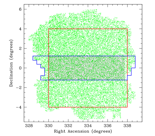
Figure 1: The angular distribution of objects in the SAS2 $r_{\rm P1}$-band source catalogues (green points). The extent of our overlapping Stripe 82 (blue line) and DR8 (red line) catalogues is also shown. The hatched zone represents the area in common to all three surveys. Coordinates are J2000.

2 The Small Area Survey

SAS2 was observed over 2 nights in the week after new moon at the beginning of July 2011. As with the real $3\pi$ survey, the exposures were split into 6 pairs of observations at different rotation angles on the sky. Ideally, each patch of sky sees a total of 12 exposures, which are then stacked to produce a deeper image. The survey is centred on $22^{\rm h}15^{\rm m}$ RA, $0{\degr}00^{\prime}$ Dec. (J2000), and the area of full coverage encompasses roughly an $8\degr\times 8\degr$ square, with a further $~{}1\degr$ wide strip around the edge with reduced coverage due to dithering. There are a total of 124 individual exposures in each band. The SDSS DR8 catalogue covers this area, whilst there is substantial overlap with the deeper SDSS Stripe 82 catalogue. Fig. 1 shows the distribution of detected sources on the sky from the stacked SAS2, together with the areas we used from the SDSS DR8 and Stripe 82 surveys (mainly restricted to areas with full SAS2 coverage in all 5 bands) . Our intercomparisons with SDSS are mainly based on the area in common to all three surveys ($\sim 16$ sq.deg.), shown as the hatched zone on Fig. 1. Fig. 2 shows the reddening distribution across the field. The mean $E(B-V)$ is $\sim 0.08$ mag, implying an $r_{\rm P1}$ extinction of $\sim 0.2$ mag, although $E(B-V)$ rises much higher to $\sim 0.26$ mag around $22^{\rm h}08^{\rm m}$ RA, $-3{\degr}30^{\prime}$ Dec.

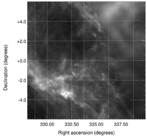
Figure 2: Greyscale map of E(B-V) reddening in the SAS2 area from the NASA/IPAC Infrared Science Archive (http://irsa.ipac.caltech.edu/applications/DUST/), derived from Schlegel et al. (1998). Black corresponds to $E(B-V)=0.01$, white to $E(B-V)=0.25$ mag.

A brief description of the PS1 camera is appropriate here. Full details can be found in Onaka et al. (2008) and Tonry & Onaka (2009). The detector consists of 60 Orthogonal Transfer Arrays (OTA), about 4800 pixels square, arranged in an $8\times 8$ pattern, excluding the four corners. OTAs are reduced independently by the PS1 pipeline software, but a few operations, e.g. photometric zero-pointing, are performed globally across the exposure. Each OTA itself consists of $8\times 8$ CCD cells about 600 pixels across, with an image scale of $\sim 0.26$ arcsec pixel^-1 (the exact scale varies with position on the camera by about 1 per cent). There are gaps between each cell of between $6$ and $8$ arcsec and larger gaps between the OTAs of about $36$ arcsec in one direction and $70$ arcsec in the other. As a result of this, and due to the dithering employed, when PS1 exposures are stacked, the resulting coverage can be very inhomogeneous.

Given the SAS2 is meant to be a demonstration of the $3\pi$ survey as a whole, the obvious question which arises is how do the properties, in particular seeing and sky brightness, of SAS2 compare with the wider $3\pi$ survey. Table 1 shows the statistics of the individual exposures which compose the SAS2. The zeropoints give the magnitude on the PS1 native system of one count (ADU) per second on the detector (for a description of how the PS1 data are photometrically calibrated, see Schlafly et al., 2012). The sky brightness and FWHM of the point spread function (PSF) come from the average value of model fits to the whole area of each individual exposure provided by the PS1 pipeline processing (the FWHM, in particular, varies with position in the focal plane). SAS2 is, in fact, extremely uniform in its properties. The rms scatter in the sky value is $\leq 0.1$ mag in all bands, whilst for FWHM it is $\leq 0.05$ arcsec. The zero points scatter by $<0.01$ mag within each band.

Table 1: Statistics of the SAS2 individual, i.e. unstacked, exposures. For comparison, the values in parenthesis for the sky brightness and FWHM represent those for all the $3\pi$ exposures taken by October 2012.

Filter	Median	Median sky	Median	Exp.	Mean
	zero pt.	brightness	FWHM	time	Airmass
	(mag)	(mag/′′2)	(′′)	(s)
$g_{\rm P1}$	$24.44$	$21.96$ $(21.95)$	$1.06$ $(1.33)$	$43$	1.25
$r_{\rm P1}$	$24.66$	$21.12$ $(20.88)$	$0.94$ $(1.19)$	$40$	1.15
$i_{\rm P1}$	$24.57$	$20.45$ $(19.79)$	$0.93$ $(1.13)$	$45$	1.09
$z_{\rm P1}$	$24.23$	$19.65$ $(19.17)$	$0.87$ $(1.08)$	$30$	1.07
$y_{\rm P1}$	$23.25$	$18.46$ $(18.30)$	$0.86$ $(0.99)$	$30$	1.08

The values for sky brightness and seeing are somewhat better than for the current $3\pi$ survey data (to October 2012), which are listed in parenthesis in Table 1. The $3\pi$ data, of course, are a much more heterogeneous sample, and the FWHM figures are skewed somewhat by a long tail to high values. The brighter skies in the redder bands are due to the fact that these bands are usually scheduled nearer full moon than was the case for SAS2. Fig. 3 shows the histogram of $r$-band FWHM for the SAS2 compared with the 3$\pi$ survey to date. The long tail to the 3$\pi$ observations is clear, although the modal seeing is only some 15 per cent higher than in SAS2. Note that we have not applied any quality cut to the 3$\pi$ data, and many of the poorer seeing observations will be not be accepted for the final survey stacks. The other bands behave in similar fashion. The trend of worse seeing at shorter wavelengths has the sign expected from atmospheric seeing, but is also believed to have a component due to the L2 corrector lens being slightly out of specification. In particular, the bluer bands suffer from a region of degraded seeing in the central half degree of the field.

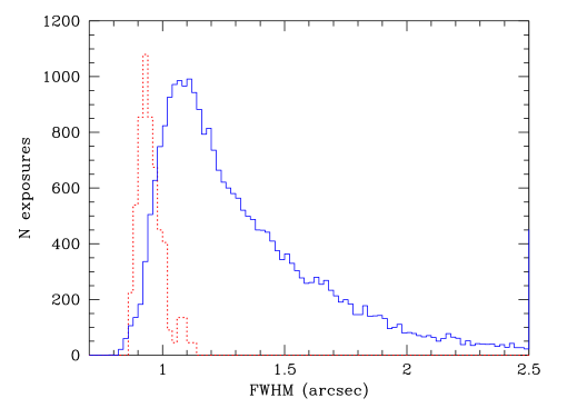
Figure 3: The distribution of mean $r$-band FWHM values for single exposures. Dashed line (red): the 124 SAS2 exposures, scaled by a factor of 45; Solid line (blue): the 26296 3$\pi$ exposures taken since the survey began. The values are averages of a model fit to the stellar profile over the whole focal plane.

Fig. 4 shows the distribution of FWHM measured on SAS2 after the stacking process, again from model fits. The median values are very similar to those of the unstacked images in Table 1, except possibly for the $y$ band, where there appears to have been a slight ($\sim 10$ per cent) degradation in image quality. We are unable to explain why this band should differ from any other, as all are treated identically in the stacking process.

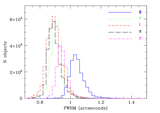
Figure 4: The distribution of model-fit FWHM values for all objects detected by the pipeline software on the SAS2 stacks. These agree well with the unstacked values (Table 1), although the $y$-band has degraded by $\sim 10$ per cent.

3 Data reduction and Analysis

3.1 IPP processing pipeline

The image processing pipeline reduction of PS1 images (IPP) is quite complex (see e.g. Magnier et al., 2006) and it is not the aim of this paper to describe these procedures in detail, but a brief overview is useful here. Once detrended and astrometrically calibrated, the individual exposures are resampled (‘warped’) on a fixed grid (a tangent plane projection) on the sky with a constant pixel size of $0.25$ arcsec (similar, but not identical to, the variable native pixel scale). This fixed grid is broken into a set of ‘skycells’, roughly $26$ arcmin across. Adjacent skycells are designed to have some overlap (to minimise issues with objects being cut by skycell boundaries, as photometry is performed independently on each skycell). Depending on the orientation and alignment of the original exposure, as many as four OTAs may contribute to one skycell. Note that because of the gaps between the CCD cells and between the OTAs, $\sim 14$ per cent of the area of each of these skycells has no data.

Skycells from different observations of the same field can then be combined to produce deeper, stacked data. Outlier rejection is applied to clean artifacts unique to individual images from the stack. As with the individual exposures, the subsequent data analysis is carried out independently on each stacked skycell.

The main data analysis routine is psphot. This constructs a model PSF for each skycell from high significance objects identified as point sources. The PSF is allowed to vary spatially over the field. The model has functional form

$$I=\frac{I_{0}}{1+kr^{2}+r^{3.33}},$$ (1)

where $r$ represents a general, radial, elliptical coordinate ($r^{2}=\frac{x^{2}}{2\sigma_{xx}^{2}}+\frac{y^{2}}{2\sigma_{yy}^{2}}+\sigma_{xy}xy$). The model is force-fit to all objects (detected at greater than $5\sigma$ significance) to produce a PSF magnitude (CAL_PSF_MAG). Fig. 5 shows how a typical example of this profile, with $k=-0.123$ (the mean $k$ for SAS2 is $-0.05$ with an rms scatter of $\pm 0.1$), differs from a Gaussian with the same FWHM ($0.85$ arcsec) and total flux. Obviously there is more power in the wings of the PS1 profile, with only $\sim 38$ per cent of the flux inside the FWHM. Even at 20 pixel ($5$ arcsec) radius the PS1 profile is still a few percent short of recovering the total flux.

Note that the IPP pipeline returns two quantities, PSF_MAJOR and PSF_MINOR, based on $\sigma_{xx}$, $\sigma_{yy}$ and $\sigma_{xy}$. For a circularly symmetric profile with $k=0$ these are by definition $0.5\times$ the FWHM of the profile (Figs. 3 and 4 use this relation). For other $k$ this is only an approximation, although for the range of $k$ found in the real data deviations are only a few percent. For example, for the PS1 profile from Fig. 5, PSF_MAJOR $=0.41$ arcsec, whereas the FWHM of the model is $0.425$ arcsec.

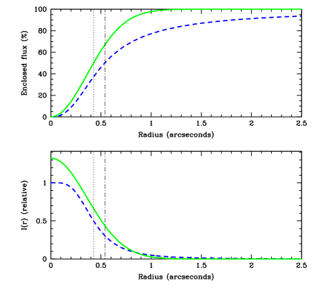
Figure 5: Top panel: the theoretical curves of growth for a Gaussian PSF (solid green line) and the model PS1 PSF described in the text with $k=-0.123$ (dashed blue line). Both profiles have the same FWHM and total intensity. The vertical dotted line indicates the radius which contains 50 per cent of the light for the Gaussian (half the FWHM), whilst the dot-dash line shows that for the PS1 profile. Bottom panel: as above, but now for the intensity profiles, $I(r)$.

Obviously the PSF model is a useful measure for point sources, but somewhat meaningless for most galaxies, so at the same time a Kron magnitude (Kron, 1980) is measured for the same objects, where the Kron flux is defined as the flux inside a circular radius of

$$r_{\rm k}=2.5\times\frac{\sum rf(i)}{\sum f(i)}$$ (2)

where the sum is taken over a series of annuli, extending to large radii (in practice, IPP uses an iterative procedure, terminating the summation at $6\times$ the radial moment found in the previous iteration), and $f(i)$ is the light distribution curve (i.e. the radial intensity profile multiplied by the area of each annulus).

The measurement of both PSF and Kron magnitudes requires a determination of the background sky. psphot constructs a sky model on a regularly spaced grid (the spacing was 400 pixels for this analysis). To do this, a histogram of a randomly selected subset of the pixels in a box of side twice the grid spacing is constructed around each grid point (there is, therefore, some correlation between adjacent points). A robust estimate of the peak is then made, which attempts to account for the skewed nature of the histogram caused by the wings of bright objects. To determine the sky at any position in the full-scale image, bilinear interpolation between the grid points is used.

Other magnitudes (e.g. model fits to extended sources) will be provided for the public release of the $3\pi$ data, but are still in the testing and development stage, and so we do not consider them further in this paper.

3.2 Simulating PS1 data

The IPP pipeline is capable of adding (and recovering) fake stars when it performs photometric analysis of an image, in order to provide an estimate of depth. However, it does not simulate galaxies, so, in order to overcome this limitation and also to provide a full independent investigation of SAS2, we generate our own fake stars and galaxies. A full description of how we construct these fakes will be given in Paper II. For this paper it is only necessary to note that we use a PS1 profile for stars (Section 3.1), and a combination of exponential disks and de Vaucouleurs profiles for galaxies, and that we generate a realistic distribution of galaxy properties, appropriate to the depth of the SAS2 images, using the mock galaxy catalogues of Merson et al. (2013), based on a $\Lambda$CDM cosmology, and the size distributions of Shen et al. (2003).

The simplest thing we can do is place these fake objects onto random backgrounds (with similar variance to real OTAs from single exposures) and try and recover them with psphot.

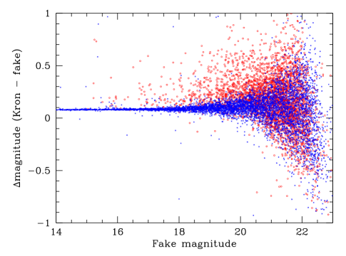
Figure 6: The difference between fake total magnitudes and Kron magnitudes returned from psphot for stars (blue crosses) and galaxies (red circles). The objects have been placed on a random background, with variance and fluxes similar to that for real $r$-band SAS2 OTAs.

Fig. 6, where we compare Kron magnitudes from psphot with the true total input magnitude for each fake object, shows the results of such a simulation based on four simulated SAS2 $r$-band OTAs, which have FWHM, mean variance, pixel masks, image scale and flux calibration identical to their real counterparts (the corresponding real OTAs, XY21/22/31/32, were chosen as those which made up SAS2 warp, 454104, which has properties typical of the survey). A numerical summary is given in Table 2. An offset is always expected, as theoretically a Kron magnitude only ever recovers a fixed fraction of the flux from an object. For a Gaussian profile, with the Kron multiplier of 2.5 used here, this fraction is $\sim 0.99$ . For the PS1 PSF, equation 1, it is slightly dependent on $k$, but for the value of $k$ used here is about 95 per cent. The measured offset is $\sim 0.06$ mag, which is very close to this prediction. For galaxies the recovered fraction should be smaller, and dependent on the particular profile of the object, being $\sim 90$ per cent for a de Vaucouleurs $r^{1/4}$ profile. Table 2 suggests our fakes have an offset of $\sim 0.2$ mag, which is slightly higher than expected.

Table 2: psphot measured Kron magnitude offsets and scatter relative to the total fake magnitude for simulated objects placed on a random background. The fluxes and variance are equivalent to those for four real $r$-band SAS2 OTAs. These are the data shown in Fig. 6.

Magnitude	$\Delta$ mag    (Kron - Fake)
(Fake)	(galaxies)	(stars)
$15-16$		$0.06\pm 0.03$
$16-17$	$0.18\pm 0.14$	$0.06\pm 0.02$
$17-18$	$0.18\pm 0.12$	$0.07\pm 0.02$
$18-19$	$0.20\pm 0.13$	$0.07\pm 0.04$
$19-20$	$0.24\pm 0.16$	$0.08\pm 0.06$
$20-21$	$0.19\pm 0.17$	$0.08\pm 0.10$
$21-22$	$0.13\pm 0.27$	$0.07\pm 0.22$

Fig. 7 shows the recovered fraction (the ‘detection efficiency’) of our fake stars and galaxies on the four simulated OTAs as a function of their input magnitude. The error bars show the rms scatter between several different realisations. We also show the results of the built-in IPP pipeline detection efficiency measurements on the the corresponding real OTAs. These are only performed for stars, but there is good agreement between our results and those from the IPP pipeline. The vertical line shows the position of the notional $5\sigma$ limit, where $\sigma$ is the measured noise inside an aperture of diameter equal to the FWHM of the PSF. This is seen to equate to a stellar detection efficiency of somewhere between 50 per cent and 60 per cent, a result we will return to in Section 3.5. The 50 per cent recovered fraction for galaxies occurs about $0.5$ mag brighter than for the stars, as might be expected given the more extended nature and hence lower surface brightness of the typical galaxy profile. The precise position of the galaxy curve is, of course, dependent on how realistic our mock galaxy catalogues are (the galaxy profiles, morphological mix and redshift distribution all play a part) - we can be more confident for the stars, where the only requirement is that we match the PS1 point spread function.

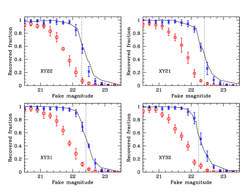
Figure 7: The fraction of fake point sources (blue stars) and galaxies (red circles) recovered by psphot from four simulated SAS2 OTAs, as a function of their simulated total magnitude. The dashed vertical line shows the magnitude of a point source which would have a flux five times the background noise inside an aperture of diameter equal to the stellar FWHM. The solid lines show the recovered fraction of fake stars as measured by the IPP pipeline processing on the corresponding real OTAs.

As a final check we now place our fakes directly onto a real SAS2 stack. Here the variance is no longer constant across the field.

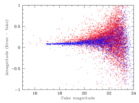
Figure 8: A comparison of the difference between input total magnitudes and measured Kron magnitudes for simulated stars (blue crosses) and galaxies (red circles) placed on a real SAS2 stack, as a function of their simulated magnitude.

Fig. 8 shows the Kron magnitudes psphot recovered from fake stars and galaxies placed on an $r$-band SAS2 stack with typical seeing, compared with their simulated total magnitudes. Table 3 summarises the comparison numerically. The magnitudes of the stars are drawn from a realistic power-law distribution, whilst the galaxies are taken from the mock catalogues discussed earlier. On the whole, psphot does a good job, and gives similar results to those for fakes on a random fake background (Table 2). Remember, as discussed earlier in this section, we expect that Kron magnitudes will always be slightly fainter than the true total magnitude, so the offsets displayed in Fig. 8 are expected. In fact, for galaxies, the offsets are nearer the theoretical expectation than they were on the fake backgrounds. There is a slight trend for objects to be measured systematically too faint as the true magnitude becomes fainter (by about $0.05$ magnitudes over the range $17<r<22$). We will return to this issue in Section 4.

Table 3: psphot measured Kron magnitude offsets and scatter relative to the total fake magnitude for $25000$ simulated stars and $38000$ simulated galaxies placed on real SAS2 $r$-band stack. These data are shown in Fig. 8.

Magnitude	$\Delta$ mag    (Kron - Fake)
(Fake)	(galaxies)	(stars)
$17-18$	$0.13\pm 0.09$	$0.06\pm 0.04$
$18-19$	$0.13\pm 0.11$	$0.07\pm 0.05$
$19-20$	$0.14\pm 0.12$	$0.08\pm 0.06$
$20-21$	$0.17\pm 0.17$	$0.09\pm 0.09$
$21-22$	$0.20\pm 0.23$	$0.10\pm 0.15$
$22-23$	$0.19\pm 0.35$	$0.12\pm 0.29$

3.3 The effects of warping and stacking

As described above, the PS1 data go through both warping and stacking stages before reaching the final data product, either of which might potentially loose depth. The warping stage, in particular, convolves the data on small scales using a Lanczos3 kernel. The effect can be seen in Fig. 9 which shows the pixel power spectrum as a function of wavenumber for an SAS2 OTA, an SAS2 warp, and, for comparison, a single SDSS field. Detected objects have been masked out before the power spectrum was computed, and for comparison purposes we have renormalised each so that they overlap at $\sim 1.5$ arcsec. The expectation from Poisson noise from sky (and read noise from the detector) would be a flat power spectrum on all scales. As expected, for the SAS2 warp we see a sharp downturn in power for scales above $k\sim 0.9$ arcsec^-1, which is due to the smoothing introduced by the warping process. The OTA and SDSS power spectra are similar at most scales - the SDSS data cuts off at a smaller wavenumber due to its larger pixel size ($0.4$ arcsec compared with $0.256$ arcsec for the PS1 OTA). Both PS1 power spectra do show small spikes at log k $\sim 0.58$ and $\sim 0.87$. We believe these are related to problems with the variable bias structure discussed further in Section 6.

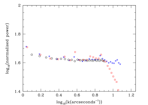
Figure 9: The pixel flux power spectrum as a function of angular wavenumber for an SAS2 chip (blue stars), and SAS2 warp (red squares) and an SDSS tile (black circles). An arbitrary renormalisation has been applied to bring the three into agreement on scales of $\sim 1.5$ arcsec. The loss of power on small scales due to the smoothing effect of the warping process is clearly visible.

To investigate the consequences of this smoothing, we consider the recovery of fake stars placed on PS1 OTAs which then go through the warping process. Note that we measure the recovered fraction as a function of simulated magnitude, and we take no account of the actual measured magnitudes of the fakes (although, in general, at the 50 per cent recovery magnitude, the offset between measured and input magnitude is $<0.1$ mag).

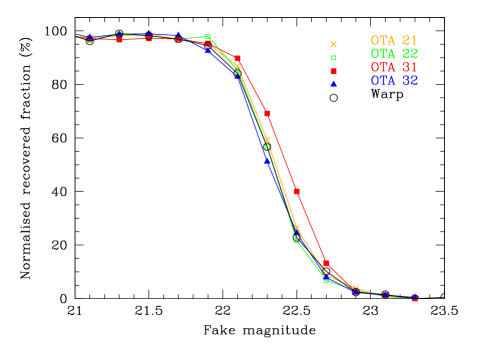
Figure 10: The percentage of fake stars recovered by psphot, as a function of input magnitude, for the four simulated OTAs, and the warp created from them. These are the same OTAs as were simulated in Fig. 7. Any loss in depth caused by the warping process would result in the warp line moving to the left of the relationships for the OTAs.

Fig. 10 shows the detection efficiency curves for our four simulated OTAs (these are the same OTAs as used in Fig. 7), and that for the warp created from these OTAs using the IPP pipeline. Note that due to the different fraction of masked pixels in each, it is necessary to normalise the curves to produce a 100 per cent recovery at bright magnitudes in order to intercompare. In an ideal world the warping process would not lose any depth, and all five curves would overlap. In practice, not all the OTAs have exactly the same noise, and they do not all contribute equal areas to the warp (OTAs XY31 and XY32 contribute slightly more area than XY21 and XY22), so it is not easy to judge. OTA XY31 is slightly deeper than the warp, but the other OTAs are not, so it seems unlikely that the warping process results in any loss of depth $\geq 0.05$ mag.

Having checked the warping procedure we now investigate the stacking procedure. The same fake stars and galaxies are added to each of the 14 warps which make up the SAS2 r-band stack 1034502 (one of which is warp 454105 which was used in the warping test). These warps are then put through the IPP stacking routine ppstack, and psphot run on the resulting stack. The fraction of the fakes recovered as a function of their fake magnitude can then be determined. This is a slightly more rigorous test then relying on the pipeline detection efficiency routine, as this puts independent fakes (i.e. at different locations on the sky) on each warp, and performs forced photometry at these locations. Obviously these cannot then be followed through the stacking process.

Fig. 11 show the results for stars. The warps, of course, are not identical, and it has been necessary to normalise each of the warp curves slightly to agree at bright magnitudes, due to the variation in masked fraction. There is also some natural variation in depth - the hatched area shows the spread in recovered fraction between them. As the mean number of warps per pixel in the resulting stack is measured to be 8.8, we would expect the stack to be $2.5\times\log{(\sqrt{8.8})}=1.18$ magnitudes fainter. This offset is shown by the arrow on Fig. 11, and is seen to be in excellent agreement with the data, so we are confident the stacking process is behaving as expected.

Fig. 12 compares the recovery of stars and galaxies on the stack. Our fake galaxies have a 50 per cent completeness about $0.4$ mag brighter than the stars. This is very slightly smaller than on the chips (Fig. 7), which presumably represents the fact that the galaxies profiles become more seeing-dominated, and hence appear star-like, at the deeper limit of the stack. Also shown is the result of running the pipeline detection efficiency routine on the equivalent real SAS2 stack. This puts fake stars directly onto the stack, rather than following them through the stacking process, but nevertheless the results are very similar.

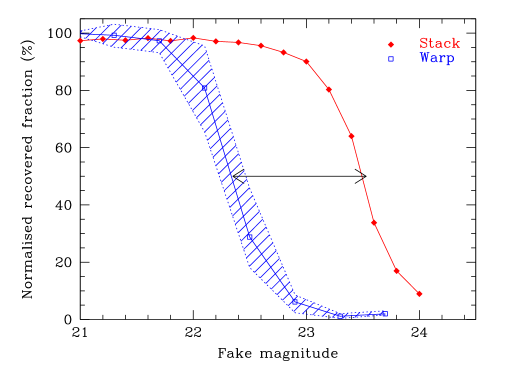
Figure 11: The mean recovered fraction of our fake stars over the 14 warps which make up our $r$-band stack ((blue, open squares), and the fraction on the stack itself (red solid diamonds), plotted as a function of their true total magnitude. The double-headed arrow shows the increased depth expected from the stacking process. The hatched zone shows the range covered by each of the 14 separate warps. Each warp has been renormalised to give a recovered fraction of 1 at $r=20.5$.

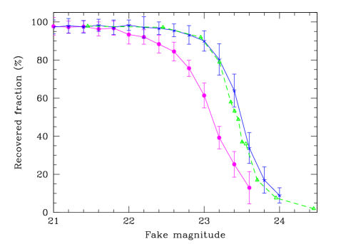
Figure 12: The recovered fraction of our fake stars (blue asterisks) and galaxies (magenta dots) on our test stack, as a function of their true magnitude. Error bars indicate the rms variation between several realisations of the fake warps which go into this stack. Also shown (green triangles, dashed line) are the fake star results from the pipeline for the equivalent PS1 stack.

3.4 Predicting the noise

We now wish to ask whether the depths of the SAS2 stacks are in line with those expected given the known properties of the camera and the conditions under which the images were taken. In this section we address whether the measured depth of SAS2 single exposures is in line with the prediction based on the measured sky and expected read-noise of the system. We define the noise per pixel of a single exposure as

$$\sigma=\sqrt{(s+d+rn^{2})}$$ (3)

where s is the flux recorded from the background sky, d the dark current accumulated during the exposure and rn the read-noise of the camera. All quantities are measured in electrons. We assume a fixed gain of $1$ e^- ADU^-1 and readnoise of $\sim 5.5$ e^- (these are typical of the values recorded in the GPC1 camera image file headers for each CCD cell). The dark current is taken to be $\sim 0.2$ e^- s^-1 (Tonry et al., 2008). In practice, all three quantities may vary by a few percent between OTAs, but we do not believe this will have any significant effect upon our analysis. The actual sky and the sky variance on each OTA are measured as part of the IPP data reduction process (after detrending).

Table 4: Predicted and measured noise levels per exposure (in ADU per pixel, assuming a gain of $1$ e^- ADU^-1), for the subset of the SAS2 which has SDSS Stripe 82 coverage. The errors come from the variation between exposures and do not indicate the accuracy to which the individual quantities can be measured on a single exposure.

Band	Measured	Predicted	Sky ADU
	$\sigma$	$\sigma$
$g_{\rm P1}$	$7.92\pm 0.04$	$8.18\pm 0.03$	$28.1\pm 0.5$
$r_{\rm P1}$	$10.11\pm 0.04$	$10.36\pm 0.04$	$69.0\pm 2.7$
$i_{\rm P1}$	$12.48\pm 0.11$	$13.09\pm 0.10$	$132.2\pm 2.6$
$z_{\rm P1}$	$12.97\pm 0.11$	$13.03\pm 0.09$	$133.6\pm 3.8$
$y_{\rm P1}$	$13.96\pm 0.10$	$14.17\pm 0.11$	$161.9\pm 3.0$

Table 4 shows the results for all the exposures used in the SAS2 which have Stripe 82 coverage (about 160 out of 600 skycells), separated by filter. The predicted values are slightly higher (up to 5 per cent) than those observed, which may suggest that the read noise and/or dark current have been slightly overestimated. However, given the uncertainties, the results are reasonably consistent, and we now go on to predict the variance expected on the stacks.

3.5 The depth of the stacks

Having seen in Sections 3.3 and 3.4 that the warping and stacking processes are reasonably well behaved, and the noise levels in single exposures are much as expected, we turn our attention to the depth of the stacked SAS2 exposures. We investigate two measures of depth: (1) the magnitude at which 50 per cent of fake stars input onto the stacks are recovered, and (2) the magnitude at which the differential number-magnitude count of all objects peaks. We would like to compare these psphot results with the expected $5\sigma$ limit for a point source inside a circular aperture of diameter equal to the FWHM. To do this it is necessary to modify the equation 3 to allow for the number of warps going into each pixel in the stacked skycell.

$$\sigma=\sqrt{((s+d+rn^{2})\times coverage)}$$ (4)

where the coverage is the average of the number of warps contributing to each pixel. Due to the construction of the camera, this coverage factor is not simply equal to the number of input warps (ideally 12 for the SAS2 and the final $3\pi$ surveys, although this number varies slightly due to the exact pattern of exposures on the sky), as $\sim 14$ per cent of the sky is lost on each warp to the gaps between the detectors (see Section 3.1). In fact, once cosmetic masking, particularly of defective CCD cells, has been taken into account the true losses can be significantly higher. As one of the IPP products is a coverage map for each stacked skycell, it is easy to determine the actual value, which turns out to be around $8.9\pm 0.9$ warps per pixel for a skycell in the central region of SAS2, where we have full coverage. This implies an average masked fraction of around 25 per cent per warp (actually, some losses may come from outlier rejection during the stacking process itself, so individual warps may not be as bad as this).

To plot the $5\sigma$ limit, we assume the idealised case of a Gaussian stellar profile, so the total flux is $2.0$ times that inside a diameter equal to the FWHM. Note, however, that the PS1 stellar profile is not Gaussian, so these $5\sigma$ limits just act as a fiducial marker, and to determine the expected absolute offset to psphot magnitudes requires the simulations in Section 3.2.

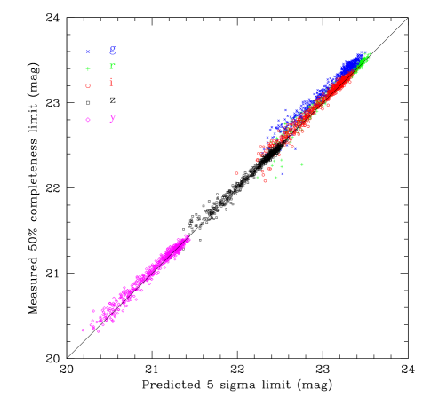
Figure 13: The simulated magnitude at which 50 per cent of fake stars injected into all the SAS2 stacks are recovered, compared with the predicted $5\sigma$ depth based on exposure time, the measured seeing, sky background and zero point, and assuming a Gaussian PSF.

There are some limitations to our analysis:

• The measured FWHM from psphot are based on a PS1 stellar image profile, although we used them to calculate the Gaussian $5\sigma$ limits. We have shown in Fig. 5 that the two are very similar. However, this uncertainty needs to be borne in mind when comparing with surveys from other telescopes. As a rough guide, a $0.1$ arcsec difference in FWHM would make a $\sim 0.1$ mag difference to our predicted $M_{5\sigma}$ limiting magnitude.

• As noted in Section 3.4 the fixed values we assume for readnoise, dark current and gain may, in practise, vary slightly from OTA to OTA. However, we believe the effect of these assumptions to be small (the exposures in the redder bands are sky-noise limited).

• We use values for the sky and sky variance which are averaged over the whole exposure, rather than for the particular OTAs which contribute to a skycell. Again we believe the effect of this to be small.

• Although we scale the variances by coverage factor, we do not account for the slight smoothing caused by the warping process. So our $5\sigma$ limits apply to an idealized, unwarped stack.

Bearing all this in mind, we now compare our predictions to the detection efficiency limits measured by the IPP pipeline. Fig. 13 shows the simulated magnitude at which 50 per cent of the fake stars injected into the stacks are recovered as a function of the predicted $5\sigma$ limit, for all five filters. The fake stars have profiles and FWHM equivalent to those measured for real stars on each stack, and vary spatially in the same fashion. The main point to take from this figure is that there is a one-to-one relationship between the two quantities which is followed by all the bands, and for different stack exposures times (the spread along the diagonal direction within each band is due mainly to differing effective stack exposures caused by the reduced coverage towards the edges of SAS2). This suggests the stacked data are all well behaved.

Due to the uncertainties already mentioned, the absolute offset between the two axes (which is close to zero) is more difficult to interpret. The points do lie reasonably close to the expectations of our simulations in Section 3.2, where we showed that the $5\sigma$ limit corresponded to a 50-60 per cent recovery fraction for fake stars. We also note that in an ideal case, cutting a sample at a magnitude equivalent to n-$\sigma$ should always result in 50 per cent of objects at that magnitude being detected. In reality the situation is more complex: (a) errors, such as those caused by the determination of the sky background, might not scatter equal numbers brightward and faintward of their true magnitude; (b) the process of detecting objects may depend on factors only indirectly related to the random noise; (c) as is the case here, the estimate of n-$\sigma$ might not perfectly match the definition used to limit the sample. However, our tests seem to show that the effects of these uncertainties are quite small, and that we do recover around 50% of objects at our idealised $5\sigma$ limit.

The detection efficiency limits are, of course, derived from fake objects put down with stellar profiles. In the real world, except near the galactic plane, most objects at these magnitude limits in the $3\pi$ survey are going to be galaxies, and so would be expected to have shallower detection limits than for point sources. It is also more appropriate to use Kron magnitudes than PSF magnitudes. So we now show in Fig. 14 the measured Kron magnitude at the which the differential number counts of all objects on each stack peaks as a function of the $5\sigma$ limit (so a comparison can be made with Fig. 13). As expected the turn-over Kron magnitudes are considerably brighter (by about $\sim 0.6$ mag) than the 50 per cent PSF magnitude limits. This comes partly from the lower detection efficiency for galaxies (see, e.g., Fig. 12) and partly because, in general, the count peak occurs at a magnitude somewhat brighter than the 50 per cent limit. The much larger scatter is probably due to the uncertainty in measuring the peak. Although the downturn in the counts is very sharp as a function of PSF magnitudes (as the sample is limited in PSF magnitude), the corresponding turn-over is much shallower as a function of Kron magnitude, due to the intrinsic spread in $\Delta(m_{\rm Kron}-m_{\rm PSF})$.

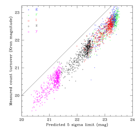
Figure 14: The Kron magnitude at which the differential object counts on the SAS2 stacks peak compared with the predicted $5\sigma$ depth based on exposure time, seeing and measured sky. The line of zero offset is provided only as a guide.

Fig. 15 shows how the average depth per skycell (in this case the 50 per cent completeness magnitude in the $r_{\rm P1}$ band) varies with position across the SAS2 field. By design, the central $8\times 8$ deg region is very uniform - as expected the depth decreases at the edges of the field where coverage is less complete. In Paper II we will investigate how the depth varies at higher spatial resolution than that of a single skycell.

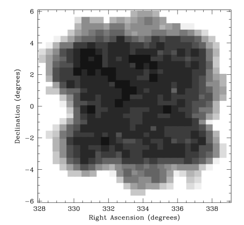
Figure 15: The spatial variation of the $r_{\rm P1}$ 50 per cent completeness limit across SAS2 (skycell by skycell). The greyscale runs from 22.5 to 23.5 in steps of 0.1 mag, light-grey to black.

4 Running psphot on SDSS pixels

Our next test is to run psphot on ten $r$-band fields from the SDSS DR8 release which are covered by SAS2, namely frame-r-004192-5-0171/72/73/74/75/87/88/89/90/91. The FWHM on these fields is about $0.9$ arcsec. We use the same parameters as used for the PS1 data, with the proviso that psphot uses a different PSF model for SDSS data than for PS1 data; specifically, $I(r)\propto(1+kr^{2}+kr^{4.5})^{-1}$. We take the photometric zero-point from the SDSS image headers. These fields cover a similar area to PS1 SAS2 skycells 1405.012/13/14. There are about 7500 objects in the DR8 catalogue to the SDSS $5\sigma$ limit.

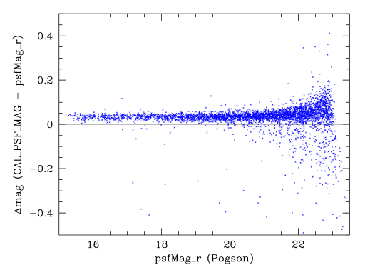
Figure 16: A comparison of PSF magnitudes measured by psphot on the 10 $r$-band SDSS fields and the DR8 catalogue psfMag magnitudes (corrected to be Pogson) for the same objects. Only objects classed as stellar in DR8 (type$=6$) are shown.

Table 5: PSF magnitude offsets and $rms$ scatter relative to SDSS DR8 Pogson-corrected psfMags, for our psphot reduction of the SDSS fields and our SAS2 data on the same region. Only objects classified as stellar in DR8 are used.These are the data shown in Figs 16. Offsets are in the sense PS1 - DR8.

DR8 mag.	$\Delta$ magnitude
($r$ Pogson)	(psphot - DR8)
$<18$	$0.03\pm 0.01$
$18-20$	$0.03\pm 0.02$
$20-21$	$0.03\pm 0.08$
$21-22$	$0.03\pm 0.04$
$22-22.5$	$0.04\pm 0.07$
$22.5-23$	$0.06\pm 0.08$

Fig. 16 shows the comparison between our reduction of the SDSS fields and the original DR8 catalogue magnitudes (converted to Pogson magnitudes from Luptitudes - this correction only has a significant effect faintward of $r\sim 22$, amounting to $0.04$ mag at $r=23$), for PSF-fitted magnitudes (in both cases) for objects classed as stellar in DR8 (type$=6$). Duplicate objects in areas of overlap between the SDSS fields have been removed. The results are summarised numerically in Table 5. The agreement is good over the whole magnitude range from $r=$ 15 – 23, with a scatter of only $\leq 0.01$ mag brightward of $r\sim 20$. There is a small offset (in the sense psphot-DR8) of $\sim 0.03$ mag, suggesting the two fitting techniques measure slightly different fluxes for the same objects. Aperture photometry on the images favours the SDSS values, so this is probably related to the amount of flux in the wings of the PSF model used by psphot. If we force psphot to adopt the usual PS1 model described in Section 3.1 which has more extended wings, we find this offset disappears, but at the expense of a 50 per cent increase in the rms scatter. Note that, in practice, if we followed the full calibration procedure used for PS1 the zero-point would change to take out the offset anyway (although this might induce an offset in the opposite direction in extended source photometry).

Apparent visually, faintward of $r\sim 22$, is a very small scale error, with the offset increasing to about $+0.06$ mag by $r\sim 23$. One possible explanation for this scale error would be if psphot measured a slightly higher sky value than SDSS, but it could also be due to differences in the PSF profile used.

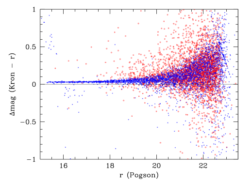
Figure 17: A comparison of Kron magnitudes measured by psphot on the 10 SDSS fields, and the DR8 catalogue Pogson-corrected modelMag values for the same objects. Blue crosses: objects classed as stellar in DR8 (type$=6$); red circles - DR8 galaxies (type$=3$).

Fig. 17 shows the corresponding plot for Kron magnitudes compared with SDSS model magnitudes. We now include galaxies as well as stars. Table 6 summarises the results. It is clear that the Kron magnitudes are not behaving as well as the PSF magnitudes, especially for stars, which now show an obvious scale error. This is in the sense that the magnitudes measured by psphot become systematically too faint at fainter SDSS magnitudes, with the offset rising from $0.02$ to $0.18$ magnitudes. Puzzlingly, neither Table 2, which shows the results of running psphot on fake stars on fake OTAs, nor Table 3, which shows the same for real stacks, show this problem to anything like this degree. And although in Section 5 we will see that the effect is present in our comparison between our SAS2 data and Stripe 82, again it is at a much lower level.

We believe the most likely explanation for such a scale error is the underestimation of the Kron radii for faint objects due to the poor signal-to-noise in the outer regions of the profile. Indeed, the measured Kron radius for stellar objects drops by about 25 per cent in the range $16<r<21$. Another possibility is that psphot is overestimating the sky background. However, tests with our fake objects suggest that, if anything, psphot slightly underestimates sky. It is unlikely that the problem lies in the DR8 modelMags, as a direct comparison between the PS1 PSF and Kron magnitudes still shows the problem. One final possibility is that many of the fainter objects classified as stars in DR8 are really galaxies, for which Kron magnitudes, as we have already noted, recover a smaller fraction of the total flux than they do for stars. This might be of consequence for the faintest bin in Table 6, but at brighter magnitudes it is fairly unambiguous what is a star and what is a galaxy. None of these potential explanations, however, offer an insight as to why the effect is so much worse on the SDSS fields.

Table 6: Kron magnitude offsets and scatter relative to SDSS DR8 Pogson-corrected modelMags, for our psphot reduction of the SDSS fields and our SAS2 data on the same region. These are the data shown in Fig. 17. Offsets are in the sense PS1 - DR8.

DR8 mag.	$\Delta$ mag.    (psphot - SDSS)
($r$ Pogson)	(galaxies)	(stars)
$<18$		$0.02\pm 0.01$
$18-20$	$0.11\pm 0.16$	$0.04\pm 0.04$
$20-21$	$0.16\pm 0.26$	$0.06\pm 0.08$
$21-22$	$0.18\pm 0.26$	$0.12\pm 0.18$
$22-22.5$	$0.17\pm 0.26$	$0.18\pm 0.30$

We now turn our interest to the depth of the psphot reduction compared to that of the DR8 catalogues. Given that the two reductions were performed on the same SDSS pixels, we would expect the counts to be very similar. We take the deeper SDSS Stripe 82 catalogue (which covers the same region of sky) as the ‘truth’, and match our detections, and those of DR8, to this, using a circular match radius of $1.0$ arcsec (the rms scatter in separation of our matched objects is only $\pm 0.1$ arcsec in both RA and Dec., so this match radius is more than adequate). We restrict the DR8 catalogue to those objects with the $r$-band BINNED_1 flag set, i.e. they are $5\sigma$ detections on the $r$-band frame, as this is the default limit of the psphot code (in practice, this made virtually no difference to our results). Fig. 18 shows the differential $r$-band number counts of matching objects, as a function of PSF-fitted magnitude.

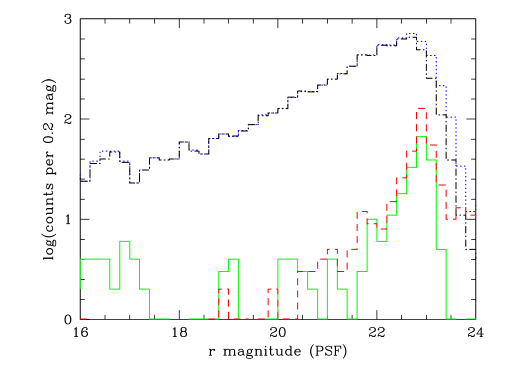
Figure 18: Differential number counts of objects on our test SDSS fields. The dot-dash (black) line shows the counts from our psphot reduction which have matching counterparts in the SDSS Stripe 82 catalogue. The dotted (blue) line shows the same matched count but now for the DR8 catalogue. Both are plotted as a function of Stripe 82 r_psfMag. The solid (green) line shows number of psphot objects which do not have a match in the Stripe 82 catalogue, as a function of CAL_PSF_MAG, whilst the dashed (red) line shows the unmatched DR8 counts as a function of DR8 r_psfMag. The offsets between Stripe 82 r_psfMag, CAL_PSF_MAG and DR8 r_psfMag are negligible.

The two data-sets show very similar counts, both dropping sharply faintward of the same magnitude limit ($r\sim 23$) to within 0.1 mag. Fig. 18 also shows the number of unmatched objects, which are presumably false detections. Again these are very similar - if anything, the psphot reduction does slightly better. We deduce from this that psphot is performing at least as well as the SDSS software.

5 Comparison with other Surveys

Having examined the internal consistency of the PS1 data, we now compare the $g$, $r$, $i$ and $z$ counts of objects in the stacked SAS2 with those from the SDSS DR8 and co-added Stripe 82 catalogues. It is necessary to remove areas, mainly around bright objects, where there are holes in the Stripe 82 catalogue. After doing this, we are left with an area in common between all three surveys of $\sim 16$ sq.deg.. We restrict the SDSS objects to those with the BINNED1 flag set to TRUE (a $5\sigma$ detection) for the band in question ($g,r,i$ and $z$).

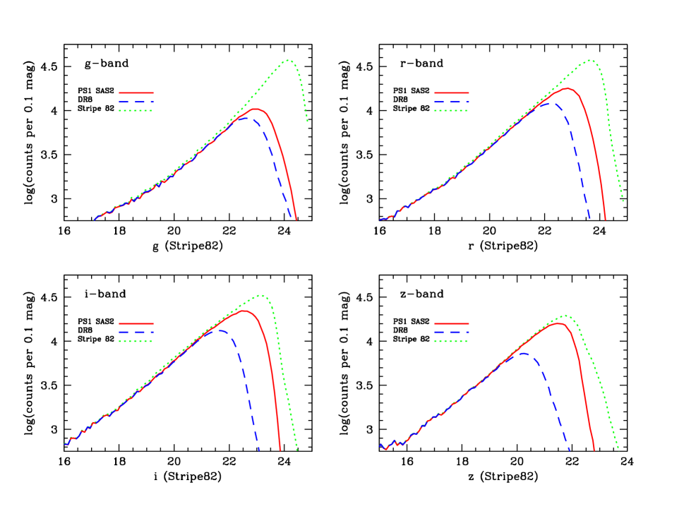
Figure 19: Differential object counts for the area in common to SAS2, DR8 and Stripe 82: green, short-dash SDSS Stripe 82; blue, long-dash SDSS DR8 with a match in Stripe 82; red, solid line PS1 stacked SAS2 with a match in Stripe 82. All three datasets are plotted as a function of Stripe 82 modelMag. Only 5-sigma detections (BINNED1 flag TRUE) are included in the SDSS data.

As an immediate indication of the depth of SAS2 and DR8 we match both to the deeper Stripe 82 data, assuming Stripe 82 to be correct (in fact there are clearly some ‘false’ sources in the Stripe 82 catalogue, but these have no effect on the number of matched objects). Again we use a circular match radius of $1.0$ arcsec. In the event of two (or more) objects in Stripe 82 being found inside this radius the brighter one is matched. The rms separation between the Stripe 82 and PS1 coordinates of all matched objects is $0.02\pm 0.15$ arcsec in RA and $-0.04\pm 0.15$ arcsec in Dec..

Table 7: Stacked SAS2 Kron magnitude offsets and scatter relative to SDSS Stripe 82 Pogson-corrected modelMags for $g$, $r$, $i$ and $z$-bands., for the whole area in common with Stripe 82. Colour corrections from Tonry et al. (2012) have been applied. The r-band data are shown in Fig. 21. Offsets are in the sense PS1 - Stripe 82. The magnitude differences have been clipped at $\pm 1.5$ mag, due to the presence of some extreme outliers.

Stripe82 mag.	Kron - $g$		Kron - $r$		Kron - $i$		Kron - $z$
(Pogson)	(galaxies)	(stars)	(galaxies)	(stars)	(galaxies)	(stars)	(galaxies)	(stars)
$16-17$							$0.15\pm 0.21$	$0.05\pm 0.03$
$17-18$	$0.07\pm 0.21$	$0.06\pm 0.03$	$0.05\pm 0.20$	$0.02\pm 0.03$	$0.10\pm 0.19$	$0.05\pm 0.04$	$0.17\pm 0.18$	$0.06\pm 0.05$
$18-19$	$0.09\pm 0.18$	$0.06\pm 0.05$	$0.05\pm 0.17$	$0.02\pm 0.05$	$0.10\pm 0.17$	$0.05\pm 0.05$	$0.18\pm 0.21$	$0.08\pm 0.06$
$18-20$	$0.10\pm 0.20$	$0.07\pm 0.06$	$0.06\pm 0.17$	$0.03\pm 0.06$	$0.12\pm 0.18$	$0.07\pm 0.07$	$0.22\pm 0.24$	$0.10\pm 0.09$
$20-21$	$0.15\pm 0.22$	$0.08\pm 0.09$	$0.09\pm 0.21$	$0.05\pm 0.10$	$0.16\pm 0.24$	$0.09\pm 0.10$	$0.23\pm 0.28$	$0.12\pm 0.15$
$21-22$	$0.18\pm 0.26$	$0.10\pm 0.14$	$0.13\pm 0.27$	$0.07\pm 0.15$	$0.18\pm 0.29$	$0.10\pm 0.17$	$0.18\pm 0.36$	$0.12\pm 0.31$
$22-23$	$0.16\pm 0.35$	$0.10\pm 0.27$	$0.11\pm 0.34$	$0.07\pm 0.27$	$0.13\pm 0.36$	$0.09\pm 0.33$

Fig. 19 shows the differential number counts of matched objects in $g$, $r$, $i$ and $z$ bands respectively, together with the Stripe 82 counts. In all cases we plot against Stripe 82 modelMag. Plotting against psfMag would move all the points $\sim 0.3$ mag fainter (the relative depths would not change), which simply reflects the fact that at the limiting depth of the SAS2 most objects are galaxies not stars, and are therefore not well measured by a PSF-fit magnitude. In all bands the SAS2 data are deeper than those from DR8, as indeed they should be, as the increase in exposure time for the stacked SAS2 ($\sim 500$ s cf $\sim 50$ s) more than compensates for the difference in telescope aperture between PS1 and Apache Point ($1.8$ m cf $2.5$ m). The camera is also more red sensitive than that used by SDSS, resulting in larger gains in the redder bands. In fact, in the $z$-band, SAS2 is nearly as deep as Stripe 82. However, a note of caution should be employed for the $3\pi$ survey as a whole - as shown in Section 2, the redder bands in SAS2 have a much fainter sky than is typical for $3\pi$, and in the seeing is somewhere better than the $3\pi$ as a whole, so the average limits may be some 0.3–0.4 mag brighter than implied here.

As there is no SDSS $y$-band, we cannot compare with Stripe 82 to determine the $y_{\rm P1}$ depth. However, we do have deeper data in the SAS2 area in the form of the PS1 Medium Deep Field 9 (MD09). The PS1 Medium Deep fields (of which there are ten) are single pointings ($\sim 7$ deg²) which are visited nightly and have longer individual exposures than the $3\pi$ (240 s for the $y$-band). The stacked $y$-band data on MD09 currently consists of over 100 of these exposures. Fig. 20 shows the counts matched to MD09 for both the SAS2 data, and, as a comparison, those from the UKIDSS LAS (Lawrence et al., 2007) DR9 release in this area. All are plotted as a function of MD09 Kron magnitude (as measured using psphot). The stacked SAS2 data are about $0.6$ magnitudes deeper than the UKIDSS LAS data, and show a count turnover at about $y_{\rm P1}$$=20.8$. It should be noted, however, that $y_{\rm P1}$, with $\lambda_{\rm eff}\sim 0.96$ ${\rm\mu m}$ is somewhat bluer that the UKIDSS $Y$-band, which stretches from 0.97–1.07 $\mu$m (Hodgkin et al., 2009).

Apart from the $y$-band, we have presented our depth estimates as function of Stripe 82 modelMag. The question naturally arises how do these compare with the SAS2 Kron magnitudes? Fig. 21 shows the $r$-band magnitude comparison between the two systems (for clarity, we only plot a random subset of 25000 out of the $\sim$440000 objects in common). Colour terms between SDSS and PS1 systems are taken from the linear relations in (Tonry et al., 2012), although for the $r$-band the correction is only of order $0.01(g-r)$. Strictly speaking these are only appropriate for main sequence stars, but they should be representative for most galaxies. Brightward of $r\sim 15.5$ saturation is an issue (probably in both datasets, but certainly in Stripe 82 as these bright stars are classified as galaxies by SDSS). Apart from that the comparison appears quite reasonable. Table 7 lists the the magnitude offsets and scatter as a function of magnitude for the $g$, $r$, $i$ and $z$ bands. As we have discussed previously, Kron magnitudes are (by definition) not expected to be total, and the amount of light lost should be larger for galaxies than for stars. Table 7 seems to bear this out, if we make the assumption that modelMags are close to total, with all the offsets showing the Kron magnitude to be fainter, and the galaxy offsets generally $0.03-0.05$ mag larger than those for the stars in all the bins, apart from the $z$ band where they are closer to $0.1$ mag. This is quite close to the theoretical expectations, given psphot uses a Kron multiplier of 2.5 (see Section 3.2). There is a slight trend for the offsets to become larger at fainter magnitudes for both stars and galaxies. As discussed in Section 4, we suspect this is due to an underestimation of the Kron radius for faint objects. In an ideal noise-free world, where the summation for the Kron radii could be extended to infinite radius, this should not happen, but in the real world we consider a shift between the two systems of only $\sim 0.05$ mag over a six magnitude range to be quite impressive.

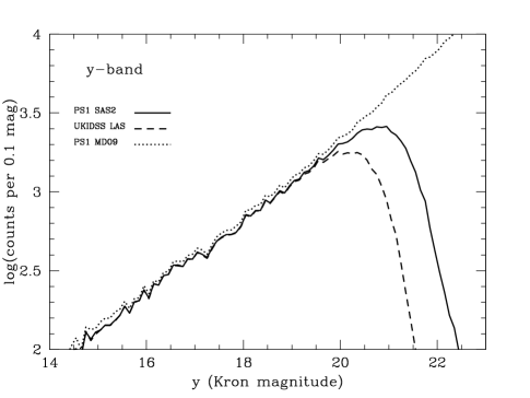
Figure 20: Differential object counts as a function of PS1 MD09 Kron magnitude for the area in common to MD09, SAS2 and UKIDSS LAS: green, dotted line MD09; blue, dashed line UKIDSS LAS with a match in MD09; red, solid line PS1 stacked SAS2 with a match in MD09.

We summarise the depth results from this section, and Section 3.5, in Table 8. For the count turnover magnitude we have used Stripe 82 modelMags, in order to aid the comparisons between the surveys, except for the $y$-band, where we use PS1 Kron magnitudes from the Medium-Deep survey. The 50 per cent point source completeness limits, being internal to PS1, are given in CAL_PSF_MAG magnitudes. The offsets between the two are in line with the expectation from Figs 13 and 14.

Table 8: Measured depths of the various surveys on the SAS2 area, as judged by the peak of the differential number-magnitude counts. The $g,r,i,z$ PS1 and DR8 data only include objects with a match in Stripe 82. Both the SDSS catalogues are restricted to objects of $5\sigma$ significance or more (BINNED1 flag TRUE) for the particular band. Also shown are the 50 per cent detection limits for point sources on the PS1 data. The PS1 results come from the stacked data. All magnitudes are SDSS Stripe 82 modelMags unless otherwise noted.

Band	PS1	PS1	DR8	Stripe 82	UKIDSS LAS
	(50%)	(count turnover magnitude)
$g$	$23.4^{*}$	23.0	22.8	24.2
$r$	$23.4^{*}$	22.8	22.2	23.6
$i$	$23.2^{*}$	22.5	21.6	23.1
$z$	$22.4^{*}$	21.7	20.3	21.8
$y$	$21.3^{*}$	$20.8^{**}$			$20.2^{**}$
∗ PS1 SAS2 PSF magnitude
∗∗ PS1 Kron magnitude from Medium Deep Field 9

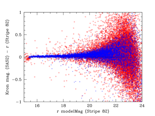
Figure 21: The difference between stacked SAS2 Kron magnitude and SDSS Stripe 82 modelMag as a function of the SDSS magnitude, for a random sample of all objects in common. Objects classified as stars by SDSS (type = 6) are blue crosses, galaxies (type = 3) are red circles. Table 7 presents the results for the whole dataset in numerical form.

6 False detections

The PS1 camera is essentially a prototype, designed for fast readout and charge shuffling (although the latter has not been implemented for the PS1 surveys), and does suffer from a variety of defects, many of which show up as false detections. This is not helped by the large number of detector edges which come from having nearly 4000 individual CCD cells. Also, with so many detectors, the decision was taken to use slightly imperfect chips, resulting in a very large saving of both cost and manufacturing time.

One particular problem has been the issue of variable dark/bias signal, which can alter on the timescale of single exposures, and on certain CCDs on a spatial scale right down to single rows. This can make accurate subtraction a challenge. We believe that the two spikes seen in the PS1 power spectra (Fig. 9) are related to this issue. There is also cross-talk between certain OTAs, persistence trails left by bright stars, and ghost images due to reflections. Efforts are ongoing to alleviate these problems. As far as the image detection software is concerned, looking back at Fig. 18 it is clear that, when run on the same pixels, psphot is no worse than SDSS at picking up false objects.

Figure 22: The location of $g$-band false detections on the sky for a typical $0.5\degr\times 0.5\degr$ area of SAS2. Left: the combination of all objects detected in all the individual exposures; right: the same area but now only for the stacked data.

Of course, the outlier clipping applied during the stacking process would be expected to remove, or at least dilute the effect of, many of the defects. This is demonstrated in Fig. 22 which shows the locations of PS1 objects with no match in Stripe 82 on a typical area of SAS2, both for all the individual exposures, and for the stacked data. The linear, diagonal feature in the individual exposures are due to defects at the edges of individual CCD cells (which often correlate between adjacent cells) which have not been masked. Most of these features disappear in the stack, as the defects in the individual exposures to not line up on the sky (due to dithering and rotation).

We investigate here how these problems affect the number of detections on the SAS2 stacks. To do this we return to the sample matched to Stripe 82 described in Section 5, but we now also consider the objects in SAS2 which have no match in Stripe 82. We exclude from this sub-sample all objects with PSF_QF_PERFECT $<0.85$ (which removes objects with more than 15 per cent of masked pixels, weighted by the PSF, whose positions may be inaccurate) and with any of the following psphot analysis FLAGS set: FITFAIL, SATSTAR, BADPSF, DEFECT, SATURATED, CR_LIMIT, MOMENTS_FAILURE, SKY_FAILURE, SKYVAR_FAILURE, SIZE_SKIPPED, which correspond to a hex flag value of 0x1003bc88. These are mainly objects for which the software has failed in some way, and so measurements are unreliable (see Table 2 of Magnier et al., 2013). This reduces the number of false detections (in all bands) by about 20-25 per cent. Remember we have already removed from the sample areas around very bright stars where there are holes in the Stripe 82 catalogue. It is likely that there are a significant number of false PS1 detections in these areas (this is not an issue unique to PS1, of course, and is presumably why there are holes in the Stripe82 catalogue in the first place). We will return to the issue of false detections around bright stars in Paper II, where we design a mask for the survey based on the positions and magnitudes of known stars. Here, we are more concerned with those defects which are peculiar to PS1 and the way the camera is constructed.

Figs 23 and 24 show the differential number counts of objects in the $r_{\rm P1}$-band, for all objects, and for those objects with and without matches in the SDSS Stripe 82 catalogue. As might be expected, the PSF unmatched counts rise sharply towards the limiting magnitude of the data, as noise spikes (and other background artefacts) start to be detected as real objects. The Kron false counts, however, tend to be more spread out, and have a lower peak (note that the integrated number of false detections is very similar - only about 5 per cent are lost due to a failure to determine a Kron magnitude). Some of this is just due to errors, but we believe a significant number of the defects, detected at low significance with the PSF fits, are extended, and so grow significantly brighter when measured with a Kron technique.

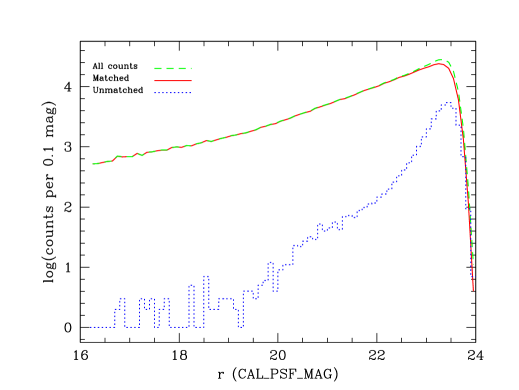
Figure 23: Differential $r_{\rm P1}$-band counts, as a function of PS1 CAL_PSF_MAG magnitude, for all objects (dashed green line), those matched Stripe 82 (solid red line) and those not matched to Stripe 82 (dotted blue line). Only 5-sigma detections (BINNED1 flag TRUE) are included in the SDSS data. Objects with any of the flags listed in the text set are excluded from the PS1 data.

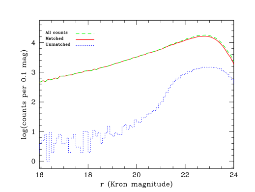
Figure 24: As Fig. 23, but now as a function of PS1 Kron magnitude.

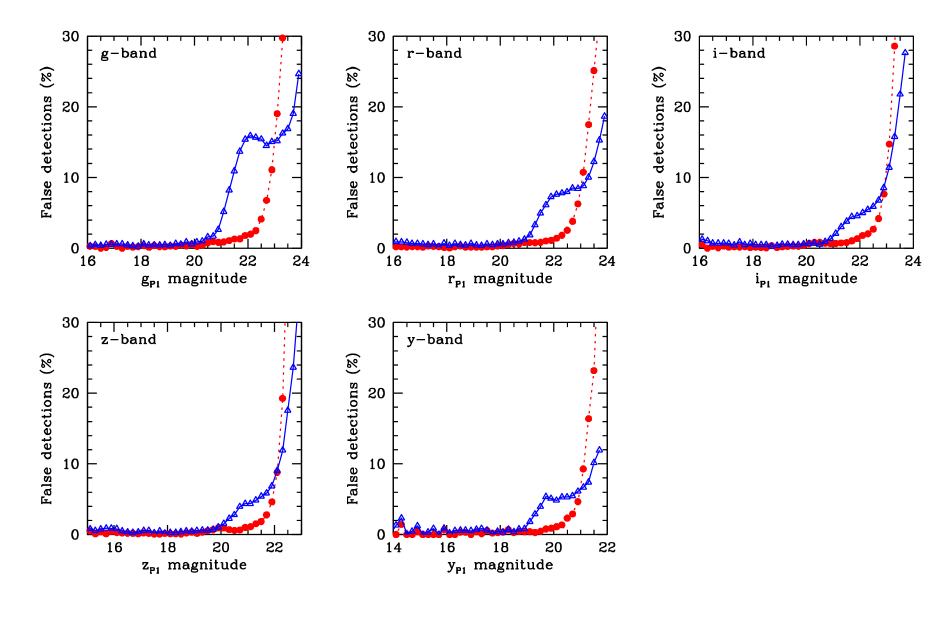
Figure 25: The percentage of detections from the stacked SAS2 data with no match to Stripe 82 ($g_{\rm P1}$, $r_{\rm P1}$, $i_{\rm P1}$, $z_{\rm P1}$) or PS1 Medium Deep Field 9 ($y_{\rm P1}$) as a function of both PSF magnitude (red circles) and Kron magnitude (blue triangles). Objects with any of the PS1 flags set which are listed in the text are excluded.

The difference between the two magnitude systems is highlighted in Fig. 25, which shows the percentage of false detections as a function of both PSF and Kron magnitudes, for $g_{\rm P1}$, $r_{\rm P1}$, $i_{\rm P1}$, $z_{\rm P1}$and $y_{\rm P1}$bands. For $y_{\rm P1}$, where there is no corresponding SDSS band, we have matched to the deeper PS1 data on Medium Deep Field 9. The $g_{\rm P1}$-band is clearly the worst - at the PSF magnitude corresponding to the 50 per cent completeness limit from Table 8 around 39 per cent of detections are false. For the Kron magnitude turnover the situation is not as bad, with only 15 per cent of objects being false, and in the $r_{\rm P1}$band the corresponding figures have dropped to 25 per cent and 8 per cent. This may reflect the fact that the $g_{\rm P1}$ exposures are more dominated by read noise than the other bands, due to the lower $g_{\rm P1}$band sky. It may also be in some part due to ghosts caused by bright stars reflecting off the surface of the detector and back off the coating on the underside of one of the correctors. These ghosts are known to strongly favour shorter wavelengths (they are virtually undetectable in $i_{\rm P1}$, $z_{\rm P1}$ or $y_{\rm P1}$). In principle, their locations can be predicted, so it should be possible to mask out most of the affected areas. Some of this is already done for the brightest stars.

7 Discussion and Conclusions

PS1 not only uses a unique camera but relies on a purpose-built software pipeline to reduce the data. We have shown, by creating fake exposures, and by adding fake objects to real exposures, that the pipeline works as expected, and that the warping and stacking processes are well behaved. The depth of the data also scales correctly with exposure time. As a further check, we have run the pipeline on SDSS fields and recovered very similar magnitudes and numbers of objects to those in the SDSS catalogues.

By matching both PS1 and SDSS DR8 datasets to SDSS Stripe82, we have determined that the SAS2 PS1 data are deeper than SDSS DR8 by $\sim 0.2$, $\sim 0.6$, $\sim 0.9$ and $\sim 1.4$ mag in $g$, $r$, $i$ and $z$ respectively. The $z$ depth is within $0.1$ mag of that of SDSS Stripe 82. As we have no external deeper $y$-band data on this field, we have had to perform an internal comparison with the PS1 Medium Deep data. We find that $y_{\rm P1}$is $\sim 0.6$ mag deeper than the UKIDSS LAS.

PSF and Kron magnitudes are being measured reliably, and agree well with SDSS, apart from a slight magnitude dependent scale error in the Kron magnitudes. This results in PS1 magnitudes becoming systematically too faint with decreasing flux, by $\sim 0.05$ mag over a $6$ magnitude range. We suspect this is due to a slight underestimation of the Kron radius at faint magnitudes, although why our reduction of the SDSS fields shows a much larger effect is a puzzle. The scatter between PS1 and Stripe 82 ranges from $\pm 0.02$ for the brightest objects in common, to about $\pm 0.3$ mag at the limit of the PS1 data.

False positives are still something of an issue for PS1, but, using the default $5\sigma$ detection threshold, are still under 15 per cent in all bands at the limiting Kron magnitude of the survey. The reduction of the SDSS fields showed a very similar number of false detections to SDSS DR8 itself, so the problems lie with the data itself not the software. The fact that the false positive rates are relatively higher in the $g_{\rm P1}$ band might be indicative that a proportion of these false detections are wavelength-dependent ghost reflections from bright stars. The false detection rate could be further reduced by insisting that objects exist in at least two bands, although this would be at the expense of limiting magnitude, and may preclude the discovery of faint, ‘drop-out’ galaxies in the redder bands. There may also be some benefit to performing forced photometry on the individual exposures at the locations of objects detected on the stacks - presumably the false detections would show inconsistent results between the exposures.

It has to be borne in mind that the SAS2 probably represents some of the best conditions that will be found in the $3\pi$ survey. It was taken under mostly dark sky conditions, even in the redder bands, which are normally taken during grey or bright time, and the seeing was $0.1-0.2$ arcsec better than the median of the existing $3\pi$ exposures. As a result, the average depth of the final stacked $3\pi$ survey cannot expected to be as good as SAS2.

In paper II we will present a simple star/galaxy separation method, calibrated using our synthetic images, and attempt to quantify the effect of the spatially varying depth across the SAS2 on the counts and angular clustering of galaxies.

For this paper we have run our own instance of the PS1 software on the pixel data, based on a build of psphot from September 2012 (software version number 34471). The data which will be released to the user community will be in the form of database access to catalogues generated by the pipeline in Hawaii. To ensure consistency, we have run extensive comparisons between our results and those currently available for SAS2 from Hawaii and find virtually identical results, so we are confident that the conclusions presented here will also apply to the initial released catalogues (the first release of the $3\pi$ survey is to be based on virtually the same pipeline code as SAS2).

References

- Abazajian et al. (2009) Abazajian K. N. et al. (The SDSS Collaboration), 2009, ApJS, 812, 543
- Aihara et al. (2011) Aihara H., Allende Prieto C., An D., et al., 2011, ApJS, 193, 29
- Annis et al. (2011) Annis L., Soares-Santos M., Strauss M. A. et al., 2011, arXiv:1111.6619
- Bertin & Arnouts (1996) Bertin E., Arnounts S., 1996, Astr. Astroph. Suppl. 117, 393
- Farrow et al. (2013) Farrow D. J. et al., 2013, MNRAS Accepted (Paper II)
- Hewett et al. (2006) Hewett P. C., Warren S. J., Leggett S. K., Hodgkin S. T., 2006, MNRAS 367, 1521
- Hodapp et al. (2004) Hodapp K. W., Siegmund W. A., Kaiser N., Chambers K., Laux U., Morgan J., Mannery E., 2004, Proc. SPIE 5489, 667
- Hodgkin et al. (2009) Hodgkin S. T., Irwin M. J., Hewett P. C., Warren S. J., 2009, MNRAS 394, 675
- Kaiser et al. (2010) Kaiser N. et al., 2010, Proc. SPIE, 7733
- Kron (1980) Kron R. G., 1980, ApJ Suppl. 43, 305
- Lawrence et al. (2007) Lawrence A. et al., 2007, MNRAS, 379, 1599
- Magnier et al. (2006) Magnier E., Kaiser N., Chambers K., 2006, Proceedings of The Advanced Maui Optical and Space Surveillance Technologies Conference, Ed.: S. Ryan, The Maui Economic Development Board, p. 455-461
- Magnier et al. (2008) Magnier E. A., Liu M., Monet D. G., Chambers K. C., 2008, IAU Symposium, 248, 553
- Magnier et al. (2013) Magnier E. A. et al., 2013, ApJ, in press
- Merson et al. (2013) Merson A. I. et al., 2013, MNRAS, 429, 556
- Onaka et al. (2008) Onaka P., Tonry J. L., Isani S., Lee A., Uyeshiro R., Rae C., Robertson L., Ching G., 2008, Proc. SPIE 7014, 12O
- Schlafly et al. (2012) Schlafly E. F. et al., 2012, ApJ 756, 158
- Schlegel et al. (1998) Schlegel D. J., Finkbeiner D. P., Davis N., 1998, ApJ, 500, 525
- Shen et al. (2003) Shen S., Mo H. J., White S. D. M., Blanton M. R., Kauffmann G., Voges W., Brinkmann J., Csabai I., 2003, MNRAS, 343, 978
- Tonry et al. (2008) Tonry J., Burke B., Isani S., Onaka P., Cooper M., 2008, Proc. SPIE, 7021
- Tonry & Onaka (2009) Tonry J., Onaka P., 2009, Proceedings of the Advanced Maui Optical and Space Surveillance Technologies Conference, Ed.: S. Ryan, p.E40.
- Tonry et al. (2012) Tonry J. L. et al.,2012, ApJ 750, 99
- York et al. (2000) York D. G., et al., 2000, AJ 120, 1579