An ALMA Survey of Submillimeter Galaxies in the Extended Chandra Deep Field-South: The AGN Fraction and X-ray Properties of Submillimeter Galaxies

Abstract

The large gas and dust reservoirs of submm galaxies (SMGs) could potentially provide ample fuel to trigger an Active Galactic Nucleus (AGN), but previous studies of the AGN fraction in SMGs have been controversial largely due to the inhomogeneity and limited angular resolution of the available submillimeter surveys. Here we set improved constraints on the AGN fraction and X-ray properties of the SMGs with ALMA and Chandra observations in the Extended Chandra Deep Field-South (E-CDF-S). This study is the first among similar works to have unambiguously identified the X-ray counterparts of SMGs; this is accomplished using the fully submm-identified, statistically reliable SMG catalog with 99 SMGs from the ALMA LABOCA E-CDF-S Submillimeter Survey (ALESS). We found 10 X-ray sources associated with SMGs (median redshift $z=2.3$), of which 8 were identified as AGNs using several techniques that enable cross-checking. The other 2 X-ray detected SMGs have levels of X-ray emission that can be plausibly explained by their star-formation activity. 6 of the 8 SMG-AGNs are moderately/highly absorbed, with $N_{\rm H}>10^{23}\ {\rm cm^{-2}}$. An analysis of the AGN fraction, taking into account the spatial variation of X-ray sensitivity, yields an AGN fraction of $17^{+16}_{-6}\%$ for AGNs with rest-frame 0.5–8 keV absorption-corrected luminosity $\geqslant 7.8\times 10^{42}$ erg s^-1; we provide estimated AGN fractions as a function of X-ray flux and luminosity. ALMA’s high angular resolution also enables direct X-ray stacking at the precise positions of SMGs for the first time, and we found 4 potential SMG-AGNs in our stacking sample.

1. Introduction

Over the past 15 yr, submillimeter (submm) and millimeter surveys have discovered a population of far-infrared (FIR) luminous, dust-enshrouded galaxies at $z>1$ (e.g., Smail et al. 1997; Ivison et al. 1998, 2000; Coppin et al. 2006; Weiß et al. 2009; Austermann et al. 2010). Multiwavelength follow-up observations of these submm galaxies (e.g., Valiante et al. 2007; Pope et al. 2008; Menéndez-Delmestre et al. 2007, 2009) have revealed that they are among the most luminous objects in the Universe (e.g., Ivison et al., 2002; Chapman et al., 2002; Kovács et al., 2006), and that they contribute significantly to the total cosmic star formation around $z\sim 2$ (e.g., Hughes et al. 1998; Barger et al. 1998; Pérez-González et al. 2005; Aretxaga et al. 2007; Hopkins et al. 2010). These submm galaxies (SMGs) typically have infrared (IR) luminosities of $\sim 10^{12}\ L_{\odot}$ or even greater, and their star formation rates (SFR) are estimated to be $\sim 100$–$1000\ M_{\odot}$yr^-1 (e.g., Kovács et al. 2006; Coppin et al. 2008; Magnelli et al. 2012). They are massive galaxies with stellar mass $M_{*}\sim 10^{11}\ M_{\odot}$ or greater (e.g., Borys et al. 2005; Xue et al. 2010; Hainline et al. 2011) and with large reservoirs of cold gas ($\gtrsim 10^{10}\ M_{\odot}$; e.g., Bothwell et al. 2013).

Most commonly found around $z\sim 2$–$3$, the volume density of SMGs is $\sim 1000$ times larger (e.g., Chapman et al. 2003, 2005; Wardlow et al. 2011) than that of the local ultraluminous infrared galaxies (ULIRGs), which are relatively rare in the local universe (e.g., Sanders & Mirabel 1996; Lonsdale et al. 2006). Also qualified as ULIRGs ($L_{\rm IR}>10^{12}\ L_{\odot}$; Sanders & Mirabel 1996), SMGs are often considered as the “distant cousins” of local ULIRGs, typically exhibiting similarly high SFR and IR luminosity. However, they also differ in some important ways. The more strongly star-forming SMGs are not simply the “scaled up” versions of local ULIRGs — for example, it appears that the star formation in SMGs occurs on a larger scale within the galaxy instead of being concentrated at the core like for the local ULIRGs (e.g., Chapman et al., 2004; Coppin et al., 2012).

Believed to be the progenitors of large local elliptical galaxies (e.g., Lilly et al. 1999; Smail et al. 2004; Chapman et al. 2005) and often involved in mergers (e.g., Tacconi et al. 2008; Engel et al. 2010; Magnelli et al. 2012), SMGs present a unique opportunity for studying the co-evolution of galaxies and their central supermassive black holes (SMBHs; $M\geqslant 10^{6}M_{\odot}$). The cosmic star formation rate and active galactic nucleus (AGN) activity both peak around $z\sim 2$ (Connolly et al., 1997; Merloni, 2004; Hopkins et al., 2007; Cucciati et al., 2012), and they appear to be related as suggested by the observed correlations between the properties of central SMBHs and their host galaxies (e.g., the $M$-$\sigma$ and the $M$-$L$ relation; Ferrarese & Merritt 2000; Gebhardt et al. 2000; Häring & Rix 2004; Gültekin et al. 2009). Moreover, simulations of galaxy evolution and SMBH growth show that merger events can trigger both star-formation activity and the onset of powerful AGN, with the peak of the AGN activity (possibly a quasar phase) coming shortly after the peak epoch of star formation (e.g., Hopkins et al. 2008; Narayanan et al. 2010). Observationally, recent studies suggest that luminous AGNs are more prevalent in massive galaxies (e.g., Xue et al. 2010; Mullaney et al. 2012) and star-forming galaxies (e.g., Rafferty et al. 2011; Santini et al. 2012; Rosario et al. 2013; Chen et al. 2013), and a very high fraction of local ULIRGs exhibit AGN activity as indicated by line-ratio diagnostics (see the review by Alonso-Herrero 2013 and references therein).

AGN activity in SMGs has been identified in previous studies through mid-IR spectroscopy (e.g., Valiante et al. 2007; Pope et al. 2008; Menéndez-Delmestre et al. 2007, 2009; Coppin et al. 2010) or X-ray (e.g., Alexander et al., 2005a, b; Pope et al., 2006; Laird et al., 2010; Lutz et al., 2010; Georgantopoulos et al., 2011; Gilli et al., 2011; Hill & Shanks, 2011; Bielby et al., 2012; Johnson et al., 2013) observations. For moderate-to-high X-ray luminosity AGNs, the X-ray emission is arguably the best AGN indicator as the hard X-rays (rest-frame energies of 2–30 keV) can penetrate through obscuration ($N_{\rm H}\lesssim$$10^{24}$ cm^-2) and also suffer less from host-galaxy contamination. However, for less X-ray luminous sources, the contribution from high mass X-ray binaries (HMXBs) in the host galaxies cannot be neglected, especially for extreme starburst galaxies like SMGs (e.g., Alexander et al. 2005b). The studies of Alexander et al. (2005a, b), Pope et al. (2006), Laird et al. (2010), Georgantopoulos et al. (2011), and Johnson et al. (2013) have all found that SMGs have a high X-ray detection rate, and a significant fraction of the X-ray detected SMGs are AGN-dominated in the X-ray band (though the exact fraction is under debate) while some are consistent with the X-ray emission being powered purely by the starburst.

All focusing on X-ray AGNs, Alexander et al. (2005a, b), Laird et al. (2010), Georgantopoulos et al. (2011), and Johnson et al. (2013) reported AGN fractions among SMGs that are consistent with each other within their 1$\sigma$ error bars. The pioneering work by Alexander et al. (2005a, b) studied the submm sources discovered by SCUBA (Holland et al., 1999) in the Chandra Deep Field North (CDF-N), which were matched to radio counterparts and spectroscopically identified (Chapman et al., 2005). They estimated the X-ray AGN fraction among SMGs to be $>38^{+12}_{-10}\%$. Laird et al. (2010), also using submm sources in the CDF-N but with Spitzer IR counterparts identified by Pope et al. (2006), reported an X-ray AGN fraction of 29%$\pm 7\%$ (or 20% if being conservative about AGN classification). Georgantopoulos et al. (2011) studied the submm sources in the Extended Chandra Deep Field South (E-CDF-S) detected by the LABOCA E-CDF-S Submm Survey (LESS; Weiß et al. 2009), which were matched to 2 Ms CDF-S (Luo et al., 2008) and 250 ks E-CDF-S (Lehmer et al., 2005) sources and also Spitzer MIPS sources (Magnelli et al., 2009), and they found an X-ray AGN fraction of $18\pm 7\%$ among the SMGs. Johnson et al. (2013) performed a direct matching between submm sources (detected at 1.1 mm by AzTEC; Wilson et al. 2008) and X-ray sources instead of first matching SMGs to IR or radio counterparts, and they found that, for SMGs in the CDF-S and CDF-N, the AGN fraction is about 28%.

Though previous studies were thorough with their statistical analyses on the reliability of counterpart matching and used supplementary IR or radio catalogs, they were largely limited by the uncertainties in finding the true X-ray counterparts of the SMGs. The submm source catalogs used in Alexander et al. (2005a, b), Laird et al. (2010), Georgantopoulos et al. (2011), and Johnson et al. (2013) are all from single-dish submm surveys, which have a typical angular resolution of $\sim 10\arcsec$–$20\arcsec$ (e.g., Chapman et al. 2005; Weiß et al. 2009). This poses great challenges for matching submm sources to the IR/radio/X-ray sources, especially when multiple multiwavelength counterparts are found within the large search apertures. Furthermore, a large fraction of the single-dish detected submm sources are actually found to resolve into multiple sources, either physically unrelated or due to the clustering of SMGs, when observed with higher angular resolution instruments such as the Submm Array (SMA) and the Atacama Large Millimeter/submm Array (ALMA; e.g., Wang et al. 2011; Barger et al. 2012; Hodge et al. 2013).

In this paper, we present the X-ray properties and the AGN fraction of the SMGs in the E-CDF-S detected by the ALMA LABOCA E-CDF-S Submm Survey (ALESS; Hodge et al. 2013; Karim et al. 2013). The ALESS is an ALMA Cycle 0 survey at 870 $\mu$m to follow up 122 of the original 126 submm sources detected by LESS, which is the largest and the most homogeneous 870 $\mu$m survey to date (Weiß et al., 2009). With the exquisite angular resolution and great sensitivity of ALMA ($\sim 1.5\arcsec$ and 3$\times$ deeper than LESS; Hodge et al. 2013), ALESS provides the first fully submm-identified sample of SMGs based on a large, contiguous, and well-defined survey (LESS), and this enables robust counterpart matching at other wavelengths. Pairing with the powerful ALESS catalog, we use the deep Chandra data in the E-CDF-S region (Lehmer et al. 2005; L05), including the most sensitive X-ray survey to date, the 4 Ms CDF-S survey (Xue et al. 2011; X11). Combining the power of Chandra and ALMA, we have unambiguously identified the X-ray counterparts by matching the X-ray sources directly onto the submm positions, which is the first among similar studies.

The AGN fractions in SMGs presented in this work are in the form of cumulative fractions as a function of X-ray flux/luminosity (i.e., the fraction of SMGs hosting AGN with X-ray flux/luminosity larger than or equal to a given value). Here we define an AGN as an accreting SMBH with any level of X-ray luminosity. Identification of an AGN inside an SMG does not mean the AGN is the main power source of the SMG or contributes significantly to the galaxy’s energy budget. Though some SMGs are quasar powered, much evidence has shown that in the majority of SMGs, star formation is the dominant energy source (e.g., Chapman et al., 2004; Alexander et al., 2005b; Pope et al., 2006). SMGs with AGN signatures (e.g., in the X-ray or IR bands) are ULIRG-AGN composites in terms of their spectral energy distributions (SEDs). Since our cumulative AGN fraction is calculated as a function of X-ray flux/luminosity, we focus on the AGNs that dominate in the X-ray band because we can measure their X-ray luminosity reliably without disentangling the contribution from host-galaxy star formation.

The paper is structured as follows: we first describe our X-ray counterpart matching for the SMGs in Section 2, and then present our analyses of their X-ray properties and also some relevant multiwavelength properties in Section 3. We have used several approaches to distinguish the X-ray AGNs from the SMGs that are star formation dominated in the X-ray (Section 4). Then we calculate the AGN fraction among the SMGs for various X-ray flux/luminosity limits (Section 5). Stacking analyses with the X-ray undetected SMGs are described in Section 6. In Section 7 we compare with previous studies, discuss our results and outlines the possible future work.

Throughout the paper, we assume a $\Lambda$CDM cosmology with $H_{0}=70.4$ km s^-1 Mpc^-1, $\Omega_{m}=0.27$, and $\Omega_{\Lambda}=0.73$ (Komatsu et al., 2011). Whenever galaxy stellar mass and SFR are involved, we assume a Salpeter initial mass function (IMF), and we have converted the quantities quoted from other works to be consistent with the Salpeter IMF whenever necessary. We use the conversion factor of $M_{\star}$ (Salpeter IMF) $=1.8\times M_{\star}$ (Kroupa or Chabrier IMF). We adopt a Galactic column density of $N_{\rm H}=8.8\times 10^{19}$ cm^-2 for the line of sight to the E-CDF-S region (e.g., Stark et al. 1992), and all reported X-ray quantities are corrected for Galactic extinction.

2. Matching X-ray Sources and Submm Sources

We first aim to find secure X-ray counterparts for the ALESS SMGs. Section 2.1 describes briefly the ALESS submm catalog from Hodge et al. (2013). Section 2.2 describes the X-ray catalogs used for finding the X-ray counterparts for the ALESS SMGs, which include additional sources beyond the L05 and X11 catalogs. Section 2.3 contains our methodology for counterpart matching (likelihood-ratio matching) and summarizes the results.

2.1. The Submm Catalog

We use the ALESS SMG catalog presented in Hodge et al. (2013) (see also Karim et al. 2013) based on ALMA follow-up observations on the submm sources detected by LESS (Weiß et al., 2009). The main-source catalog in Hodge et al. (2013) contains 99 SMGs that are within the primary beam of ALMA, with low axial ratio ($<2$), low RMS ($<0.6$ mJy) and high S/N ($>3.5$). This catalog is the first fully submm-identified, statistically reliable catalog of SMGs (Hodge et al., 2013; Karim et al., 2013).

Figure 1 shows the positions of the 99 ALESS main-catalog SMGs and the combined X-ray exposure maps for both the Chandra 4 Ms CDF-S and 250 ks E-CDF-S in gray scale. 91 of these 99 SMGs lie within the Chandra 250 ks E-CDF-S region and 44 in the 4 Ms CDF-S region. We identified 10 SMGs with X-ray counterparts (large red dots), and below we detail the X-ray catalog used and our matching method.

2.2. The X-ray Catalog

The X-ray catalog used for matching to the ALESS SMGs consists of two catalogs: one derived from the 4 Ms CDF-S data, and the other from the 250 ks E-CDF-S data. The CDF-S catalog includes (1) 776 CDF-S 4 Ms main and supplementary catalog sources (X11); and (2) 116 additional sources from a WAVDETECT catalog with a false-positive probability threshold of $<10^{-5}$ (higher than used for selecting the main and supplementary catalogs). The E-CDF-S catalog includes: (1) 795 E-CDF-S 250 ks main and supplementary catalog sources (L05); and (2) 290 additional sources from a WAVDETECT catalog with a false-positive probability threshold of $10^{-5}$. The WAVDETECT catalogs were used by X11 and L05 as master catalogs, from which they further selected sources and derived the published 4 Ms CDF-S and 250 ks E-CDF-S catalogs, respectively. Despite their relatively lower significance, the additional sources from the WAVDETECT catalogs are likely to be real X-ray sources if identified with submm counterparts, given the low density of SMGs on the sky and the excellent available positions. This has enabled us to recover genuine X-ray counterparts to the SMGs down to a lower X-ray flux limit.

Duplicate sources that are in both the CDF-S and E-CDF-S X-ray catalogs were removed. For sources in the main and supplementary catalogs of both fields, X11 has noted all duplicate sources in their published 4 Ms catalog; for the additional WAVDETECT sources, duplicate sources were identified by performing closest-counterpart matching between the two catalogs with a search radius of $1.5\arcsec$. In total, our X-ray catalog contains 892 sources in the 4 Ms CDF-S region (with 116 from the WAVDETECT lower-significance catalog), and 762 sources in the 250 ks E-CDF-S region but not in the CDF-S (with 255 from the WAVDETECT lower-significance catalog).

2.3. Source Matching

We adopted a likelihood-ratio matching method to find secure X-ray counterparts for the ALESS SMGs (e.g., Ciliegi et al. 2003; Luo et al. 2010). This method takes into account the positional uncertainties for both catalogs, as well as the expected flux distribution of the counterparts. Briefly, we computed the likelihood ratios, defined as the ratio between the probabilities of the SMG being the true counterpart and being just a background source, for all SMGs within $5\arcsec$ of an X-ray source. Then we iterate to find a likelihood-ratio cut that maximizes the sum of the matching completeness and reliability (see Luo et al. 2010 for details). We found secure X-ray counterparts for 10 ALESS SMGs with a false-match probability of 3% (i.e., an expected number of false matches of 0.3). The same 10 X-ray SMGs were recovered when a simple closest-counterpart matching method with a matching radius of $1.5\arcsec$ was adopted.

Figure 2 shows the histogram for the positional offsets between the 10 SMGs and their X-ray counterparts. The red dashed line is the estimated number of false matches as a function of the adopted matching radius for the closest-counterpart matching method. The number of false matches for a certain matching radius $r_{\rm s}$ was estimated by manually shifting the X-ray catalogs in RA and Dec by $\pm 10$–$60\arcsec$ in $10\arcsec$ increments and re-matching with the SMGs within $r_{\rm s}$. Then the number of false matches for $r_{\rm s}$ is just the average number of matches for these shifted catalogs. As shown in Figure 2, the number of false matches is much smaller than the actual number of X-ray matched SMGs at all distances $\leqslant 1.5\arcsec$ and is only 0.3 at $1.5\arcsec$. The inset plot of Figure 2 shows the histogram of offset$/\sigma_{\rm pos}$, where $\sigma_{\rm pos}$ is the quadrature sum of the positional error of each SMG and that of its matched X-ray source (i.e., $\sqrt{\sigma_{\rm submm}^{2}+\sigma_{\rm X-ray}^{2}}$). There is no SMG and X-ray source pair whose positional offset exceeds 2$\sigma_{\rm pos}$. X-ray and submm thumbnail images with illustrated positional error bars are in Figure 3.

As discussed in Section 1, when identifying X-ray counterparts for SMGs, previous studies had to invoke large search radii and/or cross-identification with radio/IR counterparts, which suffer from larger uncertainties and incompleteness (e.g., see Section 5.5 of Hodge et al. 2013). The X-ray counterparts of SMGs in our study are of high robustness, and our estimated false-match probability is more reliable and realistic. Our matching procedure does not require the assumption that sources detected in other bands such as radio or IR are very likely to be physically associated with SMGs, which is often assumed by previous studies as their search radii for counterpart matching are large. Moreover, our matching results are robust against the clustering/blending of SMGs thanks to the fully-identified ALESS SMG catalog.

The basic properties of the 10 X-ray detected SMGs are listed in Table 1. 8 of them are in the 4 Ms CDF-S region, and 9 have spectroscopic redshifts. As shown in Figure 4, their submm flux distribution (shaded blue) does not appear to differ from the distribution for all SMGs (black solid line). We performed a Kolmogorov-Smirnov (K-S) test with these two distributions and the result suggests that they share the same parent distribution, with $p=0.39$.

3. Properties of X-ray Detected SMGs

In this section, we detail our analyses and results on the X-ray properties of the X-ray detected SMGs, and other multiwavelength properties that we use in the AGN classification process (Section 4) and other following sections. We first detail the origin of the redshifts for the SMGs in Section 3.1. We then describe our analyses on the X-ray properties and present the results in Section 3.2: first for the more directly observed quantities, $\Gamma_{\rm eff}$ (effective photon index) and $L_{\rm 0.5-8\ keV}$ (rest-frame apparent luminosity), and then for the derived rest-frame intrinsic properties, $\Gamma_{\rm int}$ (intrinsic photon index), $N_{\rm H}$ (absorption column density) and $L_{\rm 0.5-8\ keV,corr}$ (absorption corrected luminosity). In Section 3.3, we describe the origins of some selected multiwavelength properties that are relevant for this work.

3.1. Redshifts

Except for ALESS 45.1, all X-ray detected SMGs have spectroscopic redshifts either from the redshift follow-up survey zLESS (Danielson et al., in prep.) or from the literature. The origins of the spectroscopic reshifts are listed in a footnote of Table 2. ALESS 45.1 has a photometric redshift (photo-z) from Simpson et al. (in prep.), which is based on optical-NIR (with photometric data from MUSYC $U,\ B,\ V,\ R,\ I,\ z,\ J,\ H,\ K$, and VIMOS $U$, HAWK-I $J$, TENIS $J,\ K_{s}$, and IRAC 3.6–8.0 $\mu$m) SED fitting using the code Hyperz (Bolzonella et al., 2000). The photo-z estimate for ALESS 45.1, $z=2.34^{+0.26}_{-0.67}$, is consistent with that from Xue et al. (2012) derived from optical-NIR SED fitting using ZEBRA (Feldmann et al., 2006). The median redshift for the X-ray detected SMGs is $z=2.3$.

Whenever reshifts are needed for the X-ray undetected SMGs in the E-CDF-S, we adopt the photo-z values from Simpson et al. (in prep.). For the 91 SMGs in the E-CDF-S, 77 have detections in $\geqslant 3$ wavebands and thus have SED fits and photo-z estimates, with a median redshift of $z=2.3$. For the remaining 14 SMGs with detections only in 0–3 wavebands, their redshifts are drawn from the likely redshift distributions estimated from simulations by Simpson et al. (in prep.). The median redshift for sources with detections in 0/1 waveband (2/3 wavebands) is $z\sim 3.5$ ($z\sim 4.5$). Simpson et al. (in prep.) estimated a median redshift of $z=2.5\pm 0.2$ for their complete sample of 96 SMGs (3 of the 99 ALESS SMGs only have IRAC coverage and are not included in their sample).

3.2. X-ray Properties

We present the X-ray properties of the 10 X-ray detected SMGs in this section. Our goal is to derive basic quantities that describe their spectral characteristics, such as the intrinsic power-law photon index $\Gamma_{\rm int}$ and the intrinsic absorption column density (neutral Hydrogen equivalent) $N_{\rm H}$ for each source, with the hope that they will help us understand the origin of the X-ray emission (see the classification of the sources in Section 4). Their X-ray spectral properties are summarized in Table 2.

The X-ray spectral analyses were done using spectra within the energy range 0.5 to 8 keV, following L05 and X11. The spectra for sources within the 4 Ms CDF-S region were extracted by X11 using ACIS Extract (AE; Broos et al. 2010). The details of the AE run can be found in X11. The spectra for the two sources that are only in the E-CDF-S region, i.e. counterparts for ALESS 66.1 and ALESS 67.1, were extracted and combined for different epochs using the CIAO (version $4.4.1$; Fruscione et al. 2006) tools specextract and combine_spectra. Their raw data were downloaded from the Chandra Data Archive and were reprocessed using the CIAO tool chandra_repro. The source extraction radii for them are twice the 90% encircled-energy aperture radii at their off-axis angles, and the background counts are estimated using 48 round regions around the source with similar or larger sizes to ensure good statistical measurements of the background counts.

3.2.1 Hardness Ratio, Effective Photon Index $\Gamma_{\rm eff}$, and Rest-Frame 0.5–8.0 keV Apparent Luminosity $L_{\rm 0.5-8\ keV}$

We first derive two simple and direct spectral characteristics: the hardness ratio, defined as the ratio of the photon count rates in the hard band (2–8 keV) and the soft band (0.5–2 keV), and the effective photon index, $\Gamma_{\rm eff}$, for a power-law model with Galactic absorption. The hardness ratios were derived using the Bayesian Estimation of Hardness Ratios (BEHR) package by Park et al. (2006). This package computes the Bayesian posterior distribution for the hardness ratios without requiring detections in both energy bands, and it is especially useful for cases with low photon counts (5 of the X-ray counterparts have less than 100 net photon counts in the 0.5–8.0 keV full band). The median of the posterior distribution is taken as the best-estimate value for the hardness ratio, and the error bars reported in Table 2 are the 68.3% (“$1\sigma$”) posterior confidence interval (CI). When the hardness ratio (or its inverse) has a posterior median of essentially zero ($<0.01$), we adopt the upper (or lower) limit value defined by the 90% posterior CI.

The effective photon index $\Gamma_{\rm eff}$ is then derived from the hardness ratio following the methods described in L05 and X11. The error bars on $\Gamma_{\rm eff}$ are estimated by converting all hardness ratios in the Bayesian posterior distribution into corresponding $\Gamma_{\rm eff}$ values then taking the 68.3% CI, as listed in Table 2. As $\Gamma_{\rm eff}$ values were derived from hardness ratios and are less directly related to the observed quantities, they are harder to constrain and therefore, following L05 and X11, for sources having low counts (see L05 and X11 for definitions) in the soft (or hard) band, we adopted the 90% CI upper (or lower) limits for $\Gamma_{\rm eff}$. For sources with low counts in both bands, we fixed $\Gamma_{\rm eff}$ to $1.4$ (following X11). Using $\Gamma_{\rm eff}$, redshift, and the observed full-band flux $f_{\rm 0.5-8\ keV}$ as listed in Table 1, we derived the rest-frame 0.5–8.0 keV apparent luminosity (with no intrinsic absorption correction; denoted as $L_{\rm 0.5-8\ keV}$ throughout this paper), for each source following the equation $L_{\rm 0.5-8\ keV}=4\pi d_{\rm L}^{2}f_{\rm 0.5-8\ keV}(1+z)^{\Gamma_{\rm eff}-2}$ (e.g., X11).

3.2.2 Intrinsic Photon Index $\Gamma_{\rm int}$, Intrinsic Absorption Column Density $N_{\rm H}$, and Rest-Frame 0.5–8.0 keV Absorption-Corrected Luminosity $L_{\rm 0.5-8\ keV,corr}$

We then estimated the intrinsic photon index, $\Gamma_{\rm int}$, the intrinsic absorption column density, $N_{\rm H}$, and the rest-frame 0.5–8.0 keV absorption-corrected luminosity (denoted as $L_{\rm 0.5-8\ keV,corr}$ throughout this paper), for each source. We used XSPEC (Arnaud, 1996) for spectral fitting and modeling. The basic model we adopted was wabs*zwabs*zpow in XSPEC, where wabs represents the Galactic absorption, zwabs represents the rest-frame intrinsic absorption ($N_{\rm H}$ being one of its parameters), and zpow is a power-law model (with index $\Gamma_{\rm int}$) in the source rest-frame.

Among the 10 X-ray detected SMGs, 5 have full-band net counts over 100 and therefore are qualified for spectral fitting. We fitted the spectra of these 5 sources without binning, and we adopted the Cash statistic (Cash 1979; cstat in XSPEC) for finding the best-fit parameters, which is well suited for fitting low-count X-ray sources and does not require any spectral binning (Nousek & Shue, 1989). Figure 5 shows the spectra of the 5 sources with full-band net counts $>$100, ALESS 11.1, 57.1, 66.1, 84.1, and 114.2, with their best-fit wabs*zwabs*zpow models, and the inset figures show the 68.3%, 90% and 99% confidence contours for $\Gamma_{\rm int}$ vs. $N_{\rm H}$. For ALESS 66.1, the plotted best-fit model is wabs*zpow, since its spectral fitting indicates no significant evidence for absorption, as illustrated by its $\Gamma_{\rm int}$-$N_{\rm H}$ contours. ALESS 114.2 does not have high photon counts (126 net counts in the full band) and exhibits high background due to its large off-axis angle in the CDF-S ($>9\arcmin$). Fixing its intrinsic photon index $\Gamma_{\rm int}$ at 1.8 (following X11; for typical AGNs) gives $N_{\rm H}\approx 2.4_{-1.2}^{+5.9}\times 10^{23}$ cm^-2. The best-fit $\Gamma_{\rm int}$ and $N_{\rm H}$ values (and 90% CI error bars) for these 5 sources are listed in Table 2 (90% CI upper limit for the $N_{\rm H}$ of ALESS 66.1).

We have also fitted the 4 obscured sources with $>$100 full-band net counts (ALESS 11.1, 57.1, 84.1 and 114.2) with a model including an Fe K$\alpha$ line, (zpow*zwabs$+$zgau)*wabs. We fixed the rest-frame line energy at 6.4 keV and width at 0.1 keV and only fitted for the normalization (line strength). We then calculated the equivalent width (XSPEC command eqw) and its 90% CI (using Markov chain Monte Carlo with the chain command). We evaluated if the model including the Fe K$\alpha$ line is statistically a better model by computing the Bayesian Information Criterion (BIC) and compared it with the BIC of the model without the Fe K$\alpha$ line (wabs*zwabs*zpow). Briefly, ${\rm BIC}=C+p\cdot\ln{n}$, where $C$ is the Cash statistic, $p$ is the number of free parameters in the model, and $n$ is the number of data points in the fit. The model with a smaller BIC value is the statistically preferred model (see Section 3.7.3 of Feigelson & Babu 2012). For ALESS 11.1, 57.1, and 114.2, the model without the Fe K$\alpha$ line is favored, and they have rest-frame equivalent widths consistent with 0 keV within 90% CI. The 90% CI upper limits on the equivalent widths for ALESS 11.1, 57.1, and 114.2 are 0.15 keV, 0.67 keV, and 0.52 keV, respectively. For ALESS 84.1, however, the model with the Fe K$\alpha$ line is slightly favored (BIC values being $494$ vs. $496$ for the model without the line), and the best-fit rest-frame equivalent width is $1.17$ keV, with a 90% CI of 0.23–2.15 keV. Since the model with the Fe K$\alpha$ line is only slightly favored for one source, ALESS 84.1, for simplicity and comparison purposes, we report the spectral analysis results using the model without the Fe K$\alpha$ line component for all sources.

For the 5 sources with full-band net counts fewer than 100, we estimated their $N_{\rm H}$ values by running simulations in XSPEC using the wabs*zwabs*zpow model with fixed $\Gamma_{\rm int}=1.8$ and varying $N_{\rm H}$ until it reproduced the observed hardness ratio (X11). For these 5 sources, spectral fittings does not provide more constraints on the X-ray properties than the simple method adopted here. An illustration of this method is in Figure 6 (similar to Figure 3 in Alexander et al. 2005b). The $N_{\rm H}$ values estimated this way are listed in Table 2 and are distinguished from the ones derived from spectral fitting by having no error bars. For ALESS 45.1 and 67.1, as their hardness ratios were given as 90% upper limits due to lack of photons in the hard band, their $N_{\rm H}$ values are therefore 90% upper limits as well.

With the best-fit or estimated $\Gamma_{\rm int}$ and $N_{\rm H}$ values for each source, we then estimated the rest-frame 0.5–8.0 keV absorption-corrected luminosity, $L_{\rm 0.5-8\ keV,corr}$, following Section 4.4 of X11, by first deriving the intrinsic full-band flux $f_{\rm 0.5-8\ keV,corr}$ using the wabs*zwabs*zpow model with $\Gamma_{\rm int}$, $N_{\rm H}$, and redshift, and then calculating $L_{\rm 0.5-8\ keV,corr}$ using the equation $L_{\rm 0.5-8\ keV,corr}=4\pi d_{\rm L}^{2}f_{\rm 0.5-8\ keV,corr}(1+z)^{\Gamma_{\rm int}-2}$. This is corrected for both Galactic and intrinsic absorption. Again, $L_{\rm 0.5-8\ keV,corr}$ estimates are 90% upper limits for ALESS 45.1 and 67.1 just as for their hardness ratios and $N_{\rm H}$ values. As noted by X11, $L_{\rm 0.5-8\ keV,corr}$ values estimated for the lower count sources typically agree within $\sim 30\%$ compared with those from direct spectral fitting, but could potentially be subject to larger uncertainties since spectral components such as reflection and scattering can play an important role for heavily obscured sources. This could also be true for the 5 sources with spectral fits, but the precision should be sufficient for the purposes of our study. For example, ALESS 73.1 is the known heavily obscured source reported by Coppin et al. (2010) and Gilli et al. (2011), who estimated $L_{\rm 2-10keV}\approx 2.5\times 10^{44}$ erg s^-1 — a bit larger than but in agreement with our estimate within a factor of two.

3.3. Multiwavelength Properties

For the classification of AGNs among SMGs described in the next section and also for the purpose of discussion, we need the rest-frame 1.4 GHz monochromatic luminosity ($L_{\rm 1.4GHz}$), the rest-frame 8–1000 $\mu$m IR luminosity ($L_{\rm IR}$) and the 40–120 $\mu$m FIR luminosity ($L_{\rm FIR}$), the stellar masses ($M_{\star}$), as well as the SFR. As we used different methods to derive SFRs in different AGN classification schemes, the SFR estimates are described in the relevant paragraphs in Section 4.2. The multiwavelength properties are listed in Table 3.

The rest-frame 1.4 GHz monochromatic luminosity, $L_{\rm 1.4GHz}$, is calculated following Alexander et al. (2003):

$$L_{\rm 1.4GHz}=4\pi d_{\rm L}^{2}f_{\rm 1.4GHz}10^{-36}(1+z)^{\alpha-1},$$ (1)

where $L_{\rm 1.4GHz}$ is in W Hz^-1, the observed 1.4 GHz radio flux $f_{\rm 1.4GHz}$ is in $\mu$Jy, and the radio spectral index is $\alpha=0.8$ (following A05). The radio counterparts and radio fluxes of the X-ray detected SMGs are from the catalog of Biggs et al. (2011) (based on Miller et al. 2008 VLA maps), identified using a closest-counterpart matching method with $r_{\rm s}=1\arcsec$ (chosen to have a false match rate $<1\%$ and also verified by visual examination; 39 SMGs are matched with radio sources).

The rest-frame IR ($8$–$1000\mu$m) luminosity $L_{\rm IR}$ and FIR (40–120 $\mu$m) luminosity were derived based on NIR-through-radio SED fitting by Swinbank et al. (in prep.). The SEDs were fitted using Spitzer, Herschel, ALMA, and VLA photometry at 3.6 $\mu$m, 4.5 $\mu$m, 5.8 $\mu$m, 8.0 $\mu$m, 24 $\mu$m, 250 $\mu$m, 350 $\mu$m, 500 $\mu$m, 870 $\mu$m and 1.4 GHz. The SED templates include the star-forming galaxy templates from Chary & Elbaz (2001) and that of SMMJ2135$-$0102 (the Eyelash galaxy; Swinbank et al. 2010).

The stellar masses for the SMGs are from Simpson et al. (in prep.). Briefly, their stellar mass estimates are derived from the absolute $H$-band photometry based on the optical-NIR SED fitting and a mass-to-light ratio based on the best-fit star formation history (either burst or constant) and stellar population synthesis models from Bruzual & Charlot (2003). Typical error bars for $M_{\star}$ are about a factor of 2 (around a factor of $\sim$3–5 if taking into account model uncertainties).

Although Simpson et al. (in prep.) only used galaxy templates in their SED fitting, AGN contamination is probably not a concern here when estimating stellar mass. Our X-ray detected SMGs have a median $\log{L_{\rm 0.5-8\ keV}}=43.0$ and all but ALESS 66.1 have $\log{L_{\rm 0.5-8\ keV}}\leqslant 43.7$ (Table 2), which is the upper-limit cut chosen by Xue et al. (2010) to minimize potential AGN contamination in the optical-NIR bands. In Section 4.6.3 of Xue et al. (2010), they studied 188 AGNs with $41.9\leqslant\log{L_{\rm 0.5-8\ keV}}\leqslant 43.7$ and examined the AGN contribution to their best-fit SED templates, the correlation of their rest-frame absolute magnitudes/colors and X-ray luminosities, and their fractions of optical-NIR emission coming from the core regions versus from the extended regions. They concluded that the AGN contamination is minimal and does not affect the optical-NIR colors or the mass estimates in a significant way. We note that, as shown in Figure 9, we do not see any correlation between $f_{\rm 0.5-8\ keV}$ and the IRAC 3.6 $\mu$m magnitude/flux of the 9 SMGs with $\log{L_{\rm 0.5-8\ keV}}\leqslant 43.7$, consistent with the findings of Xue et al. (2010).

Also, Simpson et al. (in prep.) noted that only 3 (ALESS 57.1, 66.1, 75.1) out of 77 SMGs have $\chi_{\rm red}^{2}>10$ due to 8 $\mu$m excesses indicative of AGN activity. For ALESS 57.1, the 8 $\mu$m excess feature is consistent with the fact that it is an obscured AGN. Because of its low $L_{\rm 0.5-8\ keV}$ value and non-power-law spectral shape, we do not consider that ALESS 57.1 is dominated by AGN in the optical-NIR, and we take the stellar mass estimate as reliable but caution the reader with this caveat. Since ALESS 66.1 is a known optical quasar with high $L_{\rm 0.5-8\ keV}$ and it has the worst SED fit among all sources in Simpson et al. (in prep.), we take its estimated stellar mass as less reliable and label it differently in the relevant plots involving $M_{\star}$.

4. Classifications for the X-ray Detected SMGs

In this section, we classify the 10 X-ray detected SMGs to assess if their X-ray emission reveals the existence of AGNs or if they are dominated by star formation in the X-ray regime. To do so, we exploit their X-ray properties calculated in Section 3.2 as well as other characteristics derived from their multiwavelength data (Section 3.3). We employed several independent classification methods and cross-checked between them. These methods and the derivation of the relevant multiwavelength properties used for each method are described in each of the subsections. Table 4 is a summary of the classification methods we adopted, and Table 3 lists multiwavelength properties of the X-ray detected SMGs and the classification results. Some of these methods are closely related (Method IIIa, IIIb, and IV), but we have employed all to enable cross-check between the results.

4.1. Method I & II. $\Gamma_{\rm eff}$ and X-ray Luminosity

Classification Method I. $\Gamma_{\rm eff}$: Following Alexander et al. (2005b) (A05 hereafter) and X11, we classify sources with $\Gamma_{\rm eff}<1.0$ as AGNs (see Figure 7). This hard signature of the X-ray spectrum is a feature of absorbed AGNs, as spectra having $\Gamma_{\rm eff}<1.0$ are empirically hard to explain with just the star forming component in a galaxy, which typically has $\Gamma_{\rm eff}\sim 1.5$ or even softer (e.g., Teng et al. 2005; Lehmer et al. 2008). ALESS 17.1, 57.1, 84.1, and 114.2 are classified as (obscured) AGNs under this criterion. As we adopted conservative $\Gamma_{\rm eff}$ estimates for sources with relatively low counts, some of the sources appear softer than indicated by Figure 6 because their $\Gamma_{\rm eff}$ values are upper limits or are fixed to 1.4 (e.g., ALESS 73.1). For the calculation of $\Gamma_{\rm eff}$ and the error bars and upper limits, see Section 3.2.

Classification Method II. X-ray Luminosity: Following the criterion adopted in, e.g., Bauer et al. (2004), Lehmer et al. (2008), and X11, we classify a source with rest-frame 0.5–8.0 keV absorption-corrected luminosity $L_{\rm 0.5-8\ keV,corr}$ larger than $3\times 10^{42}$ erg s^-1 as an AGN host. This is based on studies of local galaxies which found that all local star-forming galaxies have lower X-ray luminosities than $3\times 10^{42}$ erg s^-1 (e.g., Zezas et al. 2001; Ranalli et al. 2003; L10). The caveat is that the SMGs are high-redshift star-forming galaxies, and it is uncertain whether the criterion of $L_{\rm 0.5-8\ keV,corr}\geqslant 3\times 10^{42}$ established using local galaxies and AGNs would apply to these high-redshift sources. This is why we have additional classification methods (see the following sections) to ensure a reliable identification of AGNs.

Figure 7 illustrates this method, with the $y$-axis being $L_{\rm 0.5-8\ keV,corr}$. Filled circles mark the $L_{\rm 0.5-8\ keV,corr}$ values, while open circles are $L_{\rm 0.5-8\ keV}$ values. Crosses mark the $L_{\rm 0.5-8\ keV}$ (or $L_{\rm 0.5-8\ keV,corr}$) values with larger uncertainties due to fixed $\Gamma_{\rm eff}$ (or $\Gamma_{\rm int}$) as a result of having low counts. For ALESS 45.1, 67.1 and 70.1 (with crosses in open circles), $\Gamma_{\rm eff}$ values are poorly constrained due to low counts in both X-ray bands, and thus $\Gamma_{\rm eff}=1.4$ is assumed (following X11), which means their $L_{\rm 0.5-8\ keV}$ values have larger uncertainties. For sources with crosses in the filled circles, their $\Gamma_{\rm int}$ values were fixed at $1.8$ since they did not qualify for spectral fitting due to low counts, and therefore their $L_{\rm 0.5-8\ keV,corr}$ values have larger uncertainties. Arrows on the $L_{\rm 0.5-8\ keV,corr}$ of ALESS 45.1 and 67.1 indicate that these are upper limits, because their hardness ratios and $N_{\rm H}$ values were given as 90% CI upper limits (see Fig. 6 and Table 2).

All sources other than ALESS 17.1, 70.1, 67.1, and 45.1 are classified as AGNs under method II; the four sources were not classified as AGNs because their $L_{\rm 0.5-8\ keV}$ and/or $L_{\rm 0.5-8\ keV,corr}$ were relatively poorly constrained (crosses in Figure 7) and the well-constrained $L_{\rm 0.5-8\ keV}$ value was not above our threshold (for ALESS 17.1, but not the case for ALESS 73.1). We note here that the 6 sources classified as AGNs under this criterion all have $L_{\rm 0.5-8\ keV}$ values larger than $3\times 10^{42}$ erg s^-1. Therefore, if we are conservative and require $L_{\rm 0.5-8\ keV}>3\times 10^{42}$ erg s^-1 (rather than $L_{\rm 0.5-8\ keV,corr}>3\times 10^{42}$ erg s^-1) as we are dealing with high-redshift star-forming galaxies, the conclusion would still be the same.

4.2. Method III. $L_{\rm 0.5-8\ keV}$ vs. SFR

The general idea of this method is to compare the rest-frame 0.5–8.0 keV apparent luminosity, $L_{\rm 0.5-8\ keV}$, with the predicted amount as expected from the level of star formation, $L_{\rm X,SF}$. If $L_{\rm 0.5-8\ keV}$ of an SMG is $5\times$ or more than that expected from its star formation (i.e., $L_{\rm 0.5-8\ keV}\geqslant 5\times L_{\rm X,SF}$), it is classified as an AGN host (similar to the criterion adopted by A05 and X11). As detailed below, we estimated $L_{\rm X,SF}$ with two approaches, and they give consistent classification results.

Classification Method IIIa is to compare $L_{\rm 0.5-8\ keV}$ against the rest-frame 1.4 GHz monochromatic luminosity, $L_{\rm 1.4GHz}$, from which we derived a star formation rate (SFR) and $L_{\rm X,SF}$. Figure 8a illustrates this classification scheme. SMGs above the solid line ($L_{\rm 0.5-8\ keV}\geqslant 5\times L_{\rm X,SF}$) are classified as hosting AGNs. The calculation of $L_{\rm 1.4GHz}$ is described in Section 3.3. $L_{\rm X,SF}$ is derived using a correlation between $L_{\rm 1.4GHz}$ and SFR for pure starbursts or high-redshift star-forming galaxies (Equation 11 of Persic & Rephaeli 2007, PR7 for short, and references therein), and then converting SFR into $L_{\rm X,SF}$ following Lehmer et al. (2010) (L10 hereafter). The equations used are

$${\rm SFR} = L_{\rm 1.4GHz}/8.93\times 10^{20};$$ (2)

$$\log{(L_{\rm X,SF}/1.21)} = 39.49+0.74\log{\rm(SFR/1.8)},$$ (3)

where SFR is in $M_{\odot}$ yr^-1 and $L_{\rm 1.4GHz}$ is in W Hz^-1. The factor $1.8$ division of the SFR is for converting the Salpeter IMF adopted in this paper to the Kroupa IMF used by L10. The factor $1.21$ is for converting the rest-frame 2–10 keV luminosity $L_{\rm 2-10keV}$ adopted in L10 into the 0.5–8.0 keV luminosity $L_{\rm 0.5-8\ keV}$ in this paper, and it was derived with XSPEC using a simple power-law model with $\Gamma=1.5$ (e.g., Teng et al. 2005; Lehmer et al. 2008). Though there might be large scatter in conversions from $L_{\rm 1.4GHz}$ to SFR and SFR to $L_{\rm 0.5-8\ keV}$, Figure 8a clearly shows that our adopted threshold of $L_{\rm 0.5-8\ keV}>5\times L_{\rm X,SF}$ appears to be sufficient for identifying outliers in the correlation between $L_{\rm 1.4GHz}$ and $L_{\rm 0.5-8\ keV}$. Method IIIa classifies all but ALESS 17.1, 45.1 and 67.1 as AGN hosts. The results are discussed at the end of this subsection.

It is notable that all of our X-ray detected SMGs are also radio detected, whereas among all of the 99 SMGs in the ALESS main catalog, only 39 SMGs are matched with a radio source within $1\arcsec$ using the Biggs et al. (2011) radio catalog. This is perhaps not surprising, since X-ray luminosity correlates with radio luminosity for starburst galaxies like SMGs (e.g., Schmitt et al. 2006; PR07) and also the K correction is similar in the X-ray and radio bands compared to submm. Furthermore, since AGNs can also contribute significantly in the radio regime (e.g., Roy & Norris 1997; Donley et al. 2005; Del Moro et al. 2013), it is plausible that the X-ray detected SMGs are generally brighter in radio because of the extra radio flux contribution from AGNs. If this is true, then the SFR derived based on radio fluxes are over-estimated, which means that $L_{\rm X,SF}$ values are over-estimated. Since classification method IIIa would only become more conservative due to this effect, we do not attempt to correct for the AGN contribution in the radio band.

Classification Method IIIb uses less direct but tighter correlations to derive SFR and $L_{\rm X,SF}$ (see Figure 8b. The SFRs were derived following Equation 3 in Kennicutt (1998),

$${\rm SFR}=1.8\times 10^{-10}\times L_{\rm IR}/L_{\odot},$$ (4)

where SFR is in $M_{\odot}$ yr^-1 and the solar luminosity $L_{\odot}=3.9\times 10^{33}$ erg s^-1. We use the $L_{\rm IR}$ derived by Swinbank et al. (in prep.) as described in Section 3.3. We then derived $L_{\rm X,SF}$ from SFRs following L10:

$$L_{\rm X,SF}=0.67\times(9.05\times 10^{28}\cdot M_{\star}+1.62\times 10^{39}\cdot{\rm SFR}),$$ (5)

where SFR is in $M_{\odot}$ yr^-1 and the galaxy stellar mass, $M_{\star}$, is in solar masses (see Section 3.3). For SMGs which have very large SFRs, the contribution from the term $9.05\times 10^{28}\cdot M_{\star}$ is negligible ($<1\%$) except for a couple of sources. The factor $0.67$ is for converting $L_{\rm 2-10\ keV}$ into $L_{\rm 0.5-8\ keV}$ ($\times 1.21$), and for converting $M_{\star}$ as L10 adopted the Kroupa IMF ($/1.8$). This correlation has a smaller scatter than the correlation adopted in Method IIIa (see Table 4 in L10). Method IIIb gives consistent classification results as IIIa, i.e., all but ALESS 17.1, 45.1 and 67.1 are classified as AGN hosts.

To summarize the classification results under Method III, all but ALESS 17.1, 45.1 and 67.1 are classified as AGN hosts consistently under two different ways of calculating SFR and $L_{\rm X,SF}$. For the case of ALESS 17.1, however, we argue that it probably hosts an AGN based on its X-ray spectral hardness (see Section 4.1 and Fig. 7) and the results of classification Method IIIb. The apparent X-ray ‘deficit’ shown in Figure 8a is likely due to radio contribution from its AGN, and potentially also combined with the effect of gas and dust obscuration, which is consistent with its low $\Gamma_{\rm eff}$ and its high hardness ratio and $N_{\rm H}$ value (see Fig. 6, 7, and Table 2). The absorption-corrected luminosity $L_{\rm 0.5-8\ keV,corr}$ for ALESS 17.1 would put it above the classification threshold of Method IIIa (the same applies for ALESS 67.1 for both Method IIIa, b, but its $L_{\rm 0.5-8\ keV,corr}$ is an upper limit). For similar reasons, this classification criterion does not rule out the possibility of ALESS 45.1 and 67.1 hosting AGNs, though their X-ray spectral hardnesses and luminosities are consistent with them being dominated by just star-formation activity in the X-ray band.

4.3. Method IV. $f_{\rm 3.6\mu m}$ vs. $f_{\rm 0.5-8\ keV}$

We also use X-ray–to–optical/NIR flux ratio as an AGN activity indicator. In X11, sources with $\log(f_{\rm 0.5-8\ keV}/f_{R})>-1$ are classified as AGNs (e.g., Maccacaro et al. 1988; Hornschemeier et al. 2001; Bauer et al. 2004). However, as we are dealing with high-redshift ($z>1$) SMGs whose observed $R$ band corresponds to the rest-frame UV band, it is more appropriate to use a redder band to trace the stellar component. We therefore chose the IRAC Channel 1 3.6 $\mu$m band (rest-frame $J$ band for a $z=2$ source) to replace the $R$ band, and utilized the classifications of the X11 4 Ms CDF-S sources to calibrate the classification threshold for $\log(f_{\rm 0.5-8\ keV}/f_{\rm 3.6\mu m})$. The $f_{\rm 3.6\mu m}$ data for the X11 X-ray sources were compiled by X11 based on the Spitzer SIMPLE catalog (Damen et al., 2011), and the $f_{\rm 3.6\mu m}$ data for our X-ray detected SMGs are from Simpson et al. (in prep.).

Figure 9 illustrates this approach: all the X11 sources having IRAC 3.6 $\mu$m detections (643 sources; see details in Section 4.4 of X11) are plotted here with symbols representing their classifications — AGNs as red dots and galaxies as green open squares. The classifications are the same as in X11 with only one exception: the 52 sources that have $z>1$ and were classified as ‘AGN’ only under the $\log(f_{\rm 0.5-8\ keV}/f_{\rm R})>-1$ criterion in X11 are conservatively taken as galaxies here (hence the ‘AGN$-$’ and ‘Galaxy$+$’ labels in the legend). This is for the purpose of calibrating our X-ray-to–optical/NIR flux ratio threshold in a reliable and conservative way. Also, if a source is only detected in the soft or hard X-ray band and thus only has an upper limit for the full-band flux $f_{\rm 0.5-8\ keV}$ in X11, we used its soft- or hard-band flux for our calibration (i.e. a lower limit of $f_{\rm 0.5-8\ keV}$). We then looked for the $\log(f_{\rm 0.5-8\ keV}/f_{\rm 3.6\mu m})$ threshold above which a majority of the X11 sources are AGNs. For this purpose and to avoid fine-tuning, we chose $\log(f_{\rm 0.5-8\ keV}/f_{\rm 3.6\mu m})>-1$ as our classification threshold (i.e., below the solid line in Figure 9), as $\sim 95$% of the X11 sources that satisfy this criterion are AGNs.

Under this criterion, all but ALESS 17.1, 45.1 and 67.1 are classified as AGN hosts, consistent with Method III. We note here that the somewhat conservative $\log(f_{\rm 0.5-8\ keV}/f_{\rm 3.6\mu m})$ threshold we chose gives high reliability ($1-95\%=5\%$ mis-classification rate) but relatively low completeness, as $26$% of the X11 AGNs in Figure 9 actually have $\log(f_{\rm 0.5-8\ keV}/f_{\rm 3.6\mu m})<-1$.

4.4. Method V. X-ray Variability

X-ray variability is one of the distinct characteristics of AGNs, and it is an especially powerful tool for identifying highly obscured or low-luminosity AGNs where the galaxy light may dominate even in the X-ray regime. Young et al. (2012) studied 92 X-ray galaxies in the 4 Ms CDF-S, and found 20 X-ray variable galaxies that are likely to host low-luminosity AGNs. Here we follow the method in Section 3 of Young et al. (2012) and examine the variability of the 8 sources in the CDF-S.

First, we divided the CDF-S observations into four $\sim$1 Ms epochs, which can give the amount of variability each source exhibits on $\sim$month–year time scales in the observed frame. Then through Monte Carlo simulations, we calculated the probability $P$ that their variability exceeds that expected from Poisson statistics. If $P$ is less than 5%, we conclude that the source is variable.

We found that ALESS 84.1 is X-ray variable ($P=0.025$), and it has a maximum-to-minimum flux ratio of $3.1$ over the observed $10.8$ yr time frame. We were unable to conclude similarly for any of the other 7 sources in the CDF-S. This does not rule out the possibility of them being truly variable sources, since these sources have large off-axis angles (high background counts) and/or low net source counts (see Table 2), which give us relatively low statistical power when testing their variability.

4.5. Summary of Classification Results

Combining the results of all the methods described above, 8 out of the 10 X-ray detected SMGs show strong evidence of containing AGNs under at least one classification method (see Table 4). In fact, 6 of these 8 sources are classified as AGN hosts consistently under at least 3 methods. The only exception is ALESS 17.1, which is identified as an AGN host only through its spectral hardness (Method II) because its X-ray luminosity ($L_{\rm 0.5-8\ keV}$ and $L_{\rm 0.5-8\ keV,corr}$) appears to be low due to heavy intrinsic obscuration ($N_{\rm H}>10^{23}$ cm^-2; see discussion in Section 4.2).

We did not find strong AGN signatures in the X-ray for ALESS 45.1 or 67.1 using any of the methods, though it is notable that their $L_{\rm 0.5-8\ keV}$ values exceed the expected $L_{\rm X,SF}$ by a factor of $\sim$3 (see Section 7.3 for more details). They are treated as starburst dominated systems instead of ‘X-ray AGNs’ in our AGN fraction ($f_{\rm AGN}$) analysis in the next section. We note here that our classification does not rule out the possibility of ALESS 45.1 or 67.1 hosting AGNs. Future panchromatic SED analysis and/or spectroscopic study may reveal hidden or weak AGNs, or even AGNs in the X-ray undetected SMGs. For example, ALESS 45.1 actually lies within the ‘Donley wedge’ (Donley et al., 2012), which is an AGN selection scheme using the four IRAC bands and is robust for screening out high-redshift starburst galaxies (as compared to the ‘Lacy wedge’ or ‘Stern wedge’; Lacy et al. 2004, 2007; Stern et al. 2005). However, such analyses are beyond the scope of our paper as we focus on the X-ray properties of the SMGs. See more discussion in Section 7.3.

5. The AGN Fraction in Submm Galaxies

As concluded in the previous section, we classified 8 of the 10 X-ray detected SMGs as AGN hosts (SMG-AGNs). That is, among the 91 ALESS SMGs in the E-CDF-S region, 8 show X-ray signatures of AGNs. As mentioned in Section 1, this does not mean the primary energy sources of 8 SMGs are AGNs, though AGNs do dominate in the X-ray band (see discussion in Section 7.2.2). In this section, we calculate the fraction of such ‘X-ray AGNs’ among this population of SMGs in the E-CDF-S. We refer to this fraction simply as the AGN fraction, $f_{\rm AGN}$, hereafter. For a comparison between our $f_{\rm AGN}$ results and the previous ones, see Section 7.1.1.

5.1. Methodology

We follow the method discussed in Section 3.1 of Lehmer et al. (2007) and Section 5 of Silverman et al. (2008) to calculate $f_{\rm AGN}$, which takes into account the spatial inhomogeneity of the X-ray sensitivity limit across the E-CDF-S. To illustrate why such a consideration is necessary, suppose that, by chance, all ALESS SMGs lay in the least sensitive region in the E-CDF-S (the lightest gray in Figure 1, with X-ray sensitivity $>10^{-15}$ erg cm^-2 s^-1). Then only 5 SMGs would have been X-ray detected and classified as AGNs (see the X-ray flux listed in Table 1). Therefore, simply dividing the numbers of SMG-AGNs and SMGs would bias $f_{\rm AGN}$ toward either larger or smaller values depending on the spatial distribution of SMGs on an inhomogeneous X-ray sensitivity map.

The AGN fraction, $f_{\rm AGN}$, we estimated here is the flux– or luminosity–dependent cumulative fraction. That is, the $f_{\rm AGN}$ value for a certain X-ray flux/luminosity represents the fraction of SMGs that host AGNs with equal or greater X-ray flux/luminosity. We first describe how $f_{\rm AGN}$ is calculated as a function of full-band observed-frame X-ray flux ($f_{\rm 0.5-8\ keV}$; $f_{\rm X}$ for short). Following Silverman et al. (2008), the cumulative AGN fraction for SMGs hosting AGNs with X-ray flux larger than or equal to $f_{\rm X,lim}$ is

$$f_{\rm AGN}(f_{\rm X}\geqslant f_{\rm X,lim})=\sum_{i=1}^{N}\frac{1}{N_{\rm SMG,i}},$$ (6)

where $N$ is the number of SMG-AGNs with $f_{\rm X,i}\geqslant f_{\rm X,lim}$ ($f_{\rm X,i}$ being the X-ray flux of the $i^{\rm th}$ SMG-AGN); and $N_{\rm SMG,i}$ represents the number of SMGs which lie in a region with a sufficient X-ray sensitivity limit such that they would have been detected if hosting AGNs with $f_{\rm X}\geqslant f_{\rm X,i}$. Since we have 8 SMG-AGNs in the sample, naturally, we chose the $f_{\rm X,lim}$ values to be each of the 8 $f_{\rm X,i}$ values in turn. The error for $f_{\rm AGN}$ is calculated by adding in quadrature the error for each $1/N_{\rm SMG,i}$ term (estimated following Gehrels 1986). The results of $f_{\rm AGN}(f_{\rm X})$ are plotted in the upper-left panel of Figure 10.

The $f_{\rm AGN}$ values as a function of rest-frame 0.5–8.0 keV apparent luminosity, $L_{\rm 0.5-8\ keV}$ ($L_{\rm X}$ for short), or rest-frame 0.5–8.0 keV absorption-corrected luminosity, $L_{\rm 0.5-8\ keV,corr}$ ($L_{\rm X,corr}$ for short), can be calculated likewise. An additional step arises when determining whether or not the ${\rm j^{th}}$ X-ray undetected SMG at redshift $z_{\rm j}$ would have been detected if hosting an AGN with $L_{\rm X,i}$ or $L_{\rm X,corr,i}$. This additional step is to translate $L_{\rm X,i}$ or $L_{\rm X,corr,i}$ into the (hypothetical) observed flux (i.e., the same metric as the X-ray sensitivity map), assuming an AGN with $L_{\rm X,i}$ or $L_{\rm X,corr,i}$ in the ${\rm j^{th}}$ X-ray undetected SMG.

For translating $L_{\rm X,i}$ into flux, we used the equation for calculating $L_{\rm 0.5-8\ keV}$ in Section 3.2 with the redshift $z_{\rm j}$ and the $\Gamma_{\rm eff}$ value of the ${\rm i^{th}}$ SMG-AGN, $\Gamma_{\rm eff,i}$. For translating $L_{\rm X,corr,i}$ into flux, we first calculated its corresponding rest-frame apparent luminosity (absorbed), $L^{\prime}_{\rm X,i,j}$, for the hypothetical AGN with $L_{\rm X,corr,i}$ hosted by the ${\rm j^{th}}$ X-ray undetected SMG. Such a conversion requires an intrinsic column density ($N_{\rm H,j}$) assigned to each X-ray undetected SMG. To do so, we drew each $N_{\rm H,j}$ value randomly from the $N_{\rm H}$ distribution described in Section 4 of Rafferty et al. (2011), which was formulated based on the results in Tozzi et al. (2006). We then found $L^{\prime}_{\rm X,i,j}$ by calculating the ratio $L_{\rm X,corr,i}/L^{\prime}_{\rm X,i,j}$ through a simulation in XSPEC using the wabs*zwabs*zpow model with $z_{\rm j}$, $N_{\rm H,j}$, and the intrinsic photon index, $\Gamma_{\rm int,i}$, of the ${\rm i^{th}}$ SMG-AGN. Then we converted $L^{\prime}_{\rm X,i,j}$ into the observed flux in the same way as for converting $L_{\rm X,i}$ into flux as described above. The results of $f_{\rm AGN}(L_{\rm X})$ and $f_{\rm AGN}(L_{\rm X,corr})$ are shown in the middle- and lower-left panels in Figure 10.

5.2. The AGN Fractions

The black dots in the three left-hand panels of Figure 10 show the cumulative AGN fractions for the E-CDF-S ALESS SMGs. The left-most point in each panel is essentially the fraction of SMGs hosting AGNs with flux/luminosity equal to or above the current faintest SMG-AGN in X-ray ever detected in the E-CDF-S. These $f_{\rm AGN}$ values are marked in the plots and listed in Table 5.

The $f_{\rm AGN}$ analysis above is for all ALESS SMGs in the E-CDF-S. This sample of SMGs, however, may not constitute a flux-limited sample of SMGs. The reason is that ALESS differs from a regular flux-limited survey since it targeted the bright submm sources discovered by LESS. As mentioned earlier, the LESS survey is in fact a contiguous and flux-limited survey over the whole field of E-CDF-S. Thus, the LESS sources constitute a flux-limited sample for $S_{\rm 870\mu m}\geqslant 3.5$–$4.5$ mJy (LESS de-boosted flux limit; Weiß et al. 2009). Consequently, the ALESS SMGs with submm flux above the LESS flux limit are actually a flux-limited sample. We hence removed the SMGs (including SMG-AGNs) with $S_{\rm 870\mu m}<3.5$ mJy in our sample and calculated the AGN fraction for the flux-limited ($\geqslant 3.5$ mJy) SMG sample in the E-CDF-S. The results are shown in the right-hand panels of Figure 10, and the $f_{\rm AGN}$ values for the left-most points are listed in Table 5.

As expected, since brighter AGNs in general are rarer (e.g., Xue et al. 2010; Aird et al. 2012), $f_{\rm AGN}$ decreases as X-ray flux or luminosity increases for both cases with or without the submm flux cut. Also, comparing the left panels with the right panels of Figure 10, the AGN fractions for the $S_{\rm 870\mu m}\geqslant 3.5$ mJy SMG sample are larger than those for all ALESS SMGs overall. This is not surprising given that 5 out of 8 (63%) of the SMG-AGNs have flux larger than 3.5 mJy, while a smaller fraction of SMGs without AGN have $S_{\rm 870\mu m}\geqslant 3.5$ mJy (46 out of 91, 51%). However, the $f_{\rm AGN}$ values are actually consistent between the two SMG samples within the error bars.

A general trend of larger $f_{\rm AGN}$ for SMG groups with larger submm flux $S_{\rm 870\mu m}$ was also observed when we computed $f_{\rm AGN}$ as a function of $S_{\rm 870\mu m}$. It rises from about $15^{+15}_{-5}$% for $S_{\rm 870\mu m}\geqslant 1.3$ mJy (faintest ALESS SMG) to about $34^{+37}_{-17}$% for $S_{\rm 870\mu m}\geqslant 6$ mJy. However, the error bars on $f_{\rm AGN}$ are large due to the limited sample size, especially at high submm flux, and the $f_{\rm AGN}$ values are actually consistent with each other within 1$\sigma$ error bars, including the two $f_{\rm AGN}$ values at the lowest and highest $S_{\rm 870\mu m}$ ends.

The dashed lines in each panel of Figure 10 are $f_{\rm AGN}$ values if all 10 X-ray detected SMGs, including ALESS 45.1 and 67.1, are taken as AGN hosts. Note that this would only affect the $f_{\rm AGN}$ results at the low flux/luminosity end as ALESS 45.1 and 67.1 are very faint in X-ray. As we do not have strong evidence that ALESS 45.1 or 67.1 host AGN, this line can be viewed as the ‘fractions of SMGs that have X-ray flux/luminosity above certain values’ instead of cumulative AGN fractions. Future discoveries of SMG-AGNs with lower X-ray luminosities (probably involving disentangling the contributions from the star formation and AGN) will be able to push the $f_{\rm AGN}$ function to the lower $f_{\rm 0.5-8\ keV}$/$L_{\rm 0.5-8\ keV}$ ends.

6. Stacking of the X-ray Undetected SMGs

Thanks to the high-precision positions of the SMGs provided by ALESS, we are able to assess directly and reliably the average X-ray properties of the X-ray undetected SMGs through stacking. Previous works on X-ray stacking of SMGs were typically based on the positions of the IR/radio counterparts of SMGs (e.g., Laird et al. 2010; Georgantopoulos et al. 2011; Lindner et al. 2012), which, as mentioned in Section 1 and 2, suffer from the larger uncertainties in counterpart matching due to poor angular resolution of single-dish submm surveys.

To avoid poor X-ray PSF regions and high background, we only stacked sources within $7\arcmin$ of the aim points of the 4 Ms CDF-S or 250 ks E-CDF-S. SMGs within $2\times$ the 90% encircled-energy aperture radii of any X-ray sources are also not included in our stacking analysis. There are 50 sources that have small enough off-axis angles and are far enough from any X-ray sources, and only one of them lies within the 4 Ms CDF-S region; it has an effective exposure time $\sim$15 times larger than the other 49 sources in the E-CDF-S. To prevent this single source from biasing our stacking results, we did not include it in the stacking. Therefore, there are 49 SMGs in total in our stacking sample, all in the E-CDF-S region.

We follow the stacking procedures detailed in Section 3.1 of Luo et al. (2011). Briefly, we extracted the X-ray counts within an aperture of $1.5\arcsec$ in radius centered around the submm position of each of the 49 SMGs. The background counts for each SMG were estimated by extracting counts within 1000 randomly placed $1.5\arcsec$-radius apertures within $1\arcmin$ of each SMG, avoiding X-ray sources and the central SMG, and then taking the average. The total stacked counts ($S$) for these 49 SMGs are 33.5 in the soft band and 54.0 in the hard band. The stacked background counts ($B$) are 13.6 (soft) and 40.2 (hard). Thus, the net counts are 20.0 (soft) and 13.8 (hard), and the signal to noise ratios S/N ($(S-B)/\sqrt{B}$) are 5.4$\sigma$ (soft) and 2.1$\sigma$ (hard), which correspond to a probability of $p=3.7\times 10^{-6}$ for being generated by Poisson noise for the soft band, and $p=0.021$ for the hard band. The smoothed stacked images are shown in Figure 11. A summary of our stacking results can be found in Table 6.

We performed a robustness test by generating 1000 fake submm catalogs at random RA and Dec with 49 sources each (avoiding X-ray sources), and stacking them the same way as described above. None of the 1000 cases has a S/N of $\sigma\geqslant 5.4$ ($<0.1$%) in the soft band, and 21 cases ($2.1$%) have S/N of $\sigma\geqslant 2.1$ in the hard band, which are both consistent with our findings.

We then explore the possibility of identifying a sub-group of SMGs in our stacking sample that have higher probabilities of hosting AGNs and thus may contribute a significant fraction of the total stacked signal. According to our $f_{\rm AGN}$ analyses in Section 5, the expected number of SMG-AGNs in the entire ALESS SMG sample is $99\times 16\%\approx 16$ for $L_{\rm 0.5-8\ keV}\geqslant 2.63\times 10^{42}$ erg s^-1 (Table 5). That is, about 8 out of the 89 X-ray undetected SMGs are expected to host AGNs with $L_{\rm 0.5-8\ keV}\geqslant 2.63\times 10^{42}$ erg s^-1, which means for our stacking sample of 49 X-ray undetected SMGs, there would be a further $\sim$4 AGNs ($8\times 49/89$) with $L_{\rm 0.5-8\ keV}\geqslant 2.63\times 10^{42}$ erg s^-1.

Recently, Del Moro et al. (2013) identified a group of distant star-forming galaxies harboring AGNs with excess radio flux compared to their rest-frame FIR flux and SED analyses (also see similar works by Roy & Norris 1997 and Donley et al. 2005). Motivated by their work, we stacked the 4 radio-detected SMGs which have the largest rest-frame radio-to-IR luminosity ratios ($r_{\rm RI}=L_{\rm 1.4GHz}/L_{\rm IR}\times 10^{-12}$). These 4 SMGs (ALESS 2.1, 14.1, 75.1, and 122.1) also have SFR estimated using $L_{\rm 1.4GHz}$ (Equation 2) $>3$ larger than SFR estimated with $L_{\rm IR}$ (estimated using Equation 4 and $L_{\rm IR}$ values from Swinbank et al. in prep.). Figure 12 shows the histogram of the $r_{\rm RI}$ values of the 49 SMGs in our stacking sample, with the inset showing the histogram for all ALESS SMGs ($3\sigma$ flux upper limits were used when sources were not detected in radio). The X-ray stacking of these 4 SMGs yields a $7.8\sigma$ detection ($S=8.9$, $B=1.0$, $p=1.5\times 10^{-6}$) in the soft band and a $4.3\sigma$ detection ($S=10.9$, $B=3.2$, $p=6.1\times 10^{-4}$) in the hard band. These 4 SMGs (8% of the 49 stacked SMGs) contribute 46% of the total full-band net counts of the entire stacking sample (15.5 out of 33.4 photons), and their individual net counts are among the top $\sim$20% of the 49 stacked SMGs.

Using the BEHR package (Park et al. 2006; see Section 3.2.1), the hardness ratio is estimated to be $1.0^{+0.8}_{-0.5}$ (68.3% confidence interval, or “1$\sigma$” error bars), which corresponds to an effective photon index of $\Gamma_{\rm eff}=0.8^{+0.6}_{-0.5}$, following the conversion between hardness ratio and $\Gamma_{\rm eff}$ described in Section 3.2.1. After taking into account the encircled-energy fraction for our extraction aperture for each SMG and using $\Gamma_{\rm eff}=0.8$, we estimated the average X-ray flux per SMG to be $3.6\times 10^{-16}$ erg cm^-2 s^-1 in the full band ($6.3\times 10^{-17}$ erg cm^-2 s^-1 in the soft band), with a $1\sigma$ error of $\sim 50$% (flux and error calculation following L05 and X11). We note that their average full-band flux is above the sensitivity limit of the central $\sim$8$\arcmin$ region of the 4 Ms CDF-S.

Using the full-band flux estimated above and the median redshift of these 4 SMGs, $z=2.2$ (all are photometric redshifts from Simpson et al. in prep.), we estimate their average rest-frame 0.5–8.0 keV apparent luminosity to be $L_{\rm 0.5-8\ keV}=3.6\times 10^{42}$ erg s^-1. This is more than $3\times$ the amount expected just from their average star formation, $L_{\rm X,SF}\approx 1.1\times 10^{42}$ erg s^-1, estimated using their median stellar mass, $\log{M_{\star}/M_{\odot}}=11.3$, and $\mbox{SFR}=960\ M_{\odot}$yr^-1 using Equation 5 following L10. Considering their stacked X-ray luminosity and their hardness ($\Gamma_{\rm eff}=0.8$, consistent with being obscured AGNs; see Section 4.1), these 4 SMGs are likely to host AGNs (also see Figure 8).

Stacking the remaining 45 SMGs (removing the 4 radio-bright SMGs) yields a signal with $3.4\sigma$ in the soft band ($S=24.6$, $B=12.6$, $p=0.0017$) and $1.0\sigma$ in the hard band ($S=43.1$, $B=37.0$, $p=0.18$). Similar to the calculations above, we estimate the effective photon index for the stacked signal of these 45 SMGs to be $\Gamma_{\rm eff}=1.6^{+2.3}_{-1.0}$, and the average full-band flux per SMG to be $2.7\times 10^{-17}$ erg cm^-2 s^-1. Using the median redshift of these 45 SMGs, $z=2.9$, we estimate their average $L_{\rm 0.5-8\ keV}$ to be $1.2\times 10^{42}$ erg s^-1. The average $L_{\rm 0.5-8\ keV}$ is a factor of 2.4 larger than the amount of X-ray luminosity arising from just the star forming component of a typical galaxy in the sample, $L_{\rm X,SF}=4.8\times 10^{41}$ erg s^-1, estimated using their median stellar mass ($\log{M_{\star}/M_{\odot}}=10.9$) and $\mbox{SFR}=430\ M_{\odot}$yr^-1 similarly as above. This hints that additional AGNs might be in the sample, though we caution the reader that the result is tentative due to the large uncertainty on the estimated mean $L_{\rm 0.5-8\ keV}$. The error for $L_{\rm 0.5-8\ keV}$ is typically $\sim 70\%$ for the lower 1$\sigma$ error and over 100% for the upper 1$\sigma$ error (estimated using both the error from the flux, $\sim$50%, and the error from $\Gamma_{\rm eff}$ as listed above).

As mentioned earlier, there is one SMG (ALESS 10.1; with a photometric redshift of $z=2.0$ from Simpson et al. in prep.) in the 4 Ms CDF-S region that meets our stacking selection criteria but was not included in our stacking sample. We note here that this SMG is also likely to host an AGN. It has a soft band signal of $4.0\sigma$ ($S=15.4$, $B=5.7$, $p=6.0\times 10^{-4}$), a hard band signal of $2.2\sigma$ ($S=26.6$, $B=17.4$, $p=0.024$), and a full-band signal of $3.9\sigma$ ($p=2.6\times 10^{-4}$). It was not included in our X-ray catalog because its false-positive probability is larger than $10^{-5}$ (see Section 2.2). We estimate its $L_{\rm 0.5-8\ keV}$ to be $5.3\times 10^{43}$ erg s^-1, which is significantly beyond the expected X-ray luminosity arising just from its star formation ($L_{\rm X,SF}=6.0\times 10^{41}$ erg s^-1, estimated in the same way as above using its redshift, $z=2.0$, its stellar mass, $\log{M_{\star}/M_{\odot}}=10.6$, and $\mbox{SFR}=550\ M_{\odot}$yr^-1).

7. Discussion

We have presented the X-ray properties and AGN fractions of the X-ray detected ALESS SMGs in the E-CDF-S region, as well as our X-ray stacking results, in the previous sections. We compare our results with those of the previous studies in Section 7.1 below, and compare the X-ray and relevant multiwavelength properties and the AGN fraction of our SMG sample with other populations in Section 7.2. We revisit the two X-ray detected SMGs that are not classified as AGNs, ALESS 45.1 and 67.1, and discuss the origin of their X-ray emission in Section 7.3. In Section 8, we discuss possible future works.

7.1. Comparison with Previous Studies

In this section, we compare our study and results with four previous studies of X-ray AGNs in SMGs by A05, Laird et al. (2010; La10), Georgantopoulos et al. (2011; G11), and Johnson et al. (2013; J13). We first compare the AGN fraction, X-ray detection rate, and stacking results, and then we explore the reasons behind the similarities and differences between the results by comparing the submm/X-ray catalogs and methodologies used in the previous studies and ours.

7.1.1 The AGN Fraction among SMGs

Our AGN fraction, $f_{\rm AGN}$, results are presented in Figure 10 and Table 5. A direct comparison between our results and those of A05, La10, G11 and J13 is also shown in Figure 10, where the AGN fraction estimates from these four studies are plotted with red letters. The $x$-axis values of the red letters are the X-ray flux or luminosity of the faintest SMG-AGNs in these four previous studies (all converted into the 0.5–8.0 keV energy range assuming $\Gamma_{\rm eff}=1.4$ or $\Gamma_{\rm int}=1.8$ when necessary). The quoted error bars on their AGN fraction estimates are typically a few to ten percent, which is roughly reflected by the size of the red letters. The error bars are not plotted for clarity of presentation and also because they are likely to be underestimated due to the large uncertainty in counterpart matching and their simple methods of computing $f_{\rm AGN}$ values (see Section 7.1.4 for details). Taking these factors into account, our $f_{\rm AGN}$ estimates agree with the estimates in previous studies, especially for the $f_{\rm AGN}$ results for SMGs with $S_{\rm 870\mu m}>3.5$ mJy shown in the right panels of Figure 10, considering the differences in the submm catalogs (see Section 7.1.4).

To be specific, the estimated $f_{\rm AGN}$ values are: $38^{+12}_{-10}\%$ in A05 (75$\pm 19\%$ for the radio-selected SMGs); $(20$–$29)\pm 7$% in La10 (29% if 3 ambiguous sources are counted as AGNs; the plotted value is 24.5%); 18$\pm 7$% in G11 (for the sources in the CDF-S only and no E-CDF-S sources, which is more appropriate for comparison here); and $\sim$28% in J13.

The AGN fraction reported by A05 appears higher than the rest (though consistent within 1$\sigma$ error bars), potentially due to the fact that many of their SMGs were discovered via specific targeting of radio sources. Radio-detected SMGs seem to have a higher AGN fraction than the general SMG population, suggesting that the A05 result is potentially biased towards high AGN fraction, as also noted by A05, L10, and G11. The findings of A05 (a high AGN fraction among radio SMGs with heavy obscuration) are also consistent with the stacking analysis by Lindner et al. (2012), who studied radio-selected SMGs and found Fe K$\alpha$ line emission with high equivalent width.

Among the 20 radio SMGs in Alexander et al. (2005a) and A05 (selected for being radio sources), 15 (75$\pm 19$%) are identified as AGNs; and among the 21 radio-detected SMGs in the ALESS catalog and in the CDF-S region, 6 (29$\pm 12$%) are identified to be AGNs. The reason why our number (29%) is lower than that of A05 (75%) could be that the radio data associated with our work are deeper (ours: Biggs et al. 2011 down to $\sim$15 $\mu$Jy at $3\sigma$; A05: Richards 2000; Chapman et al. 2004 down to $\sim$24 $\mu$Jy at $3\sigma$), which would imply that brighter radio sources are more likely to host AGN.

To test this, we performed an $f_{\rm AGN}$ analysis on the radio-detected SMGs. For all radio-detected SMGs in our sample (36 SMGs), the AGN fraction is typically a factor of 2–3 larger than that for the entire ALESS sample at any given flux/luminosity limit. If we apply a radio flux cut of 40 $\mu$Jy (to match with the radio depth of A05), then the AGN fraction is a factor of 2.5–4 larger than that of all ALESS SMGs, and also larger than the AGN fraction for that of all radio-detected SMGs. Thus, it seems that AGN fraction increases with increasing radio flux. However, the results are tentative due to limited source statistics.

We emphasize that our AGN-fraction results are more reliable, and our reported error bars are more realistic values than previous studies because of our superb submm/X-ray data and the analysis method adopted. We explain in details in Section 7.1.4.

7.1.2 The X-ray Detection Rate of SMGs

As mentioned in Section 5.2, the dashed lines in Figure 10 can be taken as the ‘fraction of SMGs that have X-ray flux/luminosity above certain values’ instead of AGN fractions. As indicated by the upper-left panel of Figure 10, the fraction of ALESS SMGs that have $f_{\rm 0.5-8\ keV}>7.7\times 10^{-17}$ erg cm^-2 s^-1 (the $f_{\rm 0.5-8\ keV}$ of ALESS 45.1) could be as much as 50% or even higher (1$\sigma$ lower limit; the actual fraction is estimated to be 100% due to the small number of X-ray detected SMGs at the faint end).

Our X-ray detection rate estimate for the SMG population (dashed line in Figure 10) is consistent within 1–2$\sigma$ with the previous studies, especially considering the different X-ray depths and methodologies. For the previous studies with the X-ray data from the 2 Ms CDF-N: A05 reported an X-ray detection rate of $85^{+15}_{-20}\%$ among their radio-detected SMG sample, and La10 reported 45$\pm 8$%. For the studies with the X-ray data from the 4 Ms CDF-S: G11 reported 26$\pm 9\%$, and J13 reported 34% (both for the sources within CDF-S only). We note that even for studies in the same X-ray field, the numbers are likely for different X-ray depths, because their SMG samples differ and their faintest X-ray detected SMGs are of different X-ray fluxes.

Overall, we confirm the high X-ray detection rate of SMGs as reported in previous studies.

7.1.3 Comparison of Stacking Results

This work is the first to perform X-ray stacking directly at the precisely known position of SMGs. All previous studies were aided by the positions of the multiwavelength counterparts of SMGs and thus suffer larger uncertainties. Thus, we caution the reader that the comparison presented in this section is not a completely direct one.

The works of A05 and Lindner et al. (2012) perhaps suffer the least from positional uncertainties and mismatches, as they were both based on radio-selected SMGs. A05 stacked 3 SMGs that are X-ray undetected in their sample, and found marginal detections in the soft and full bands, with an estimated rest-frame 0.5–8 keV luminosity of $L_{\rm 0.5-8\ keV}=2\times 10^{42}$ erg s^-1 at median redshift $z=2.1$. This is consistent with our result stacking all 49 SMGs in our stacking sample, with $L_{\rm 0.5-8\ keV}=1.2\times 10^{42}$ erg s^-1 at median $z=2.6$, especially considering the error bars for $L_{\rm 0.5-8\ keV}$ ($\gtrsim 70\%$, see Section 6). The work by Lindner et al. (2012) stacked 38 SMGs in the Lockman Hole, and also obtains a detection in the soft band. They estimated $L_{\rm 0.5-8\ keV}$ to be $4.4\times 10^{42}$ erg s^-1 based on their X-ray stacking in the rest-frame of the SMGs (converted from rest-frame 2–8 keV luminosity assuming $\Gamma_{\rm eff}=1.5$). Considering the median SFR of SMGs is around 500 $M_{\odot}$ yr^-1(for the 49 SMGs in our stacking sample) with expected $L_{\rm 0.5-8\ keV}=5.5\times 10^{41}$ erg s^-1, the stacked mean $L_{\rm 0.5-8\ keV}$ values from this work, A05, and Lindner et al. (2012) all have X-ray excesses relative to the amount expected form just star formation. Especially for A05 and Lindner et al. (2012), which are both on radio-selected SMGs, the excesses appear to be larger.

If such X-ray excesses are real, this suggests that there are AGNs in the stacking samples. In Section 6, we mentioned that there are potentially 4 AGN candidates among our stacking sample of 49 SMGs selected via rest-frame radio-luminosity excesses. Lindner et al. (2012) also conclude that there is strong evidence supporting an AGN presence in their sample based on the detection of strong Fe K$\alpha$ line emission (with high equivalent width $>1$ keV), which corroborates the results of the rest-frame spectral analyses by A05 on the most obscured group of SMG-AGNs (see Figure 7 of A05). These stacking results are broadly consistent with the fact the radio-selected SMGs seem to have a large AGN fraction, as mentioned in Section 7.1.1.

The stacking analyses by La10 and G11 report $L_{\rm 0.5-8\ keV}=6\times 10^{41}$ erg s^-1 and $L_{\rm 0.5-8\ keV}=4\times 10^{41}$ erg s^-1, respectively (both at $z=2.1$; both converted into 0.5–8 keV rest-frame energies assuming $\Gamma_{\rm eff}=1.5$). These are lower than the results of A05 and Lindner et al. (2012) and also our stacking results, though still consistent within 1$\sigma$ error bars considering the large uncertainty associated with $L_{\rm 0.5-8\ keV}$. However, their stacking analyses were based on IRAC (La10) and MIPS (G11) positions, which could suffer source mismatches and larger positional uncertainties (see the next subsection). It is perhaps not surprising that these two stacking analyses yield such a level of stacked X-ray luminosity, regardless of correct matching onto SMGs, since the IRAC or MIPS detected galaxies are usually moderately or even highly star-forming galaxies. It is also plausible that the $L_{\rm 0.5-8\ keV}$ values in La10 and G11 are lower than ours because IRAC/MIPS selected sources have a lower SFR on average and perhaps also a lower AGN fraction.

7.1.4 Comparison of Catalogs and Methodologies

We have mentioned above that compared to previous studies, our work provides the most reliable estimates of AGN fraction (as well as X-ray fraction) and realistic error bars thanks to our superior submm/X-ray catalogs and the methodology adopted. We describe in detail these differences between our work and previous studies below.

First, the superb angular resolution ($\sim$1$\arcsec$) and great sensitivity ($\lesssim 1.5$ mJy at 3.5$\sigma$) of ALMA has enabled us to identify unambiguously the X-ray counterparts to the SMGs with high confidence for the first time among similar works. Due to a larger false-positive rate, source blending, and the poor positional precision in the previous generation submm surveys, earlier studies suffer from large uncertainty in their analyses. As an illustration of this issue, we compare with the submm sources and their X-ray counterparts identified in G11: among the 14 X-ray counterparts in G11, 7 are not recovered in our study, and we find 3 more true X-ray counterparts that are not in G11 (ALESS 17.1, 70.1, and 73.1). We note these 3 additional matches are all submm bright ($>$4 mJy), and therefore this addition is not because our submm catalog (ALESS) is deeper than previous ones, which are typically at a limit of 3–4 mJy. ALESS 17.1 and 73.1 are discovered with X-ray counterparts due to the improvement of X-ray catalog depth (the 4 Ms Chandra catalog by X11 in this work, compared with the 2 Ms in Luo et al. 2008 used in G11). ALESS 70.1 is matched with an X-ray source due to its improved submm position. Such a large discrepancy in source matching could indicate that our agreement on the AGN fraction with G11 (and possibly also other similar studies) could be, at least partially, coincidental.

Secondly, the X-ray catalog we used includes data derived from the deepest X-ray survey — the 4 Ms CDF-S, while previous studies mostly used the 2 Ms CDF-N (A05; La10) or the 2 Ms CDF-S (G11). We also went beyond the main catalogs of L05 and X11 and included the sources from the supplementary catalogs and even the additional sources from the candidate WAVDETECT catalogs used by L05 and X11 (see Section 2.2 for details). This has enabled us to provide as many reliable X-ray counterparts to the SMGs as possible.

Finally, we adopted the ‘1/$N$’ method for our AGN fraction or X-ray detection rate analyses, which corrects for the bias introduced by the inhomogeneous X-ray sensitivity coverage in the E-CDF-S region (see Section 5.1). In comparison, the AGN fractions reported in the previous studies are derived from simply dividing the number of AGNs by the number of SMGs. Our method has enabled us to report $f_{\rm AGN}$ values in terms of fractions of AGNs above certain X-ray flux/luminosity limits, which is a more well-defined and meaningful way to report such quantities when there are large variations in X-ray sensitivity.

7.2. Comparison between the SMG-AGNs
and Other Populations

In this section, we compare the SMG-AGNs with other SMGs, galaxies and AGNs/quasars. Section 7.2.1 provides a context for the SMGs and SMG-AGNs among other galaxies and AGNs at similar redshifts by presenting them in the commonly used color-mass diagram. Section 7.2.2 discusses the similarities and differences between the SMG-AGNs and the general X-ray AGNs/QSOs. Section 7.2.3 compares the AGN fractions in SMGs and local ULIRGs, with cautions on the differences between these two populations.

7.2.1 SMGs in the Color-Mass Diagram

We first place the SMGs in the context of other galaxies and the X-ray detected AGNs in the CDF-S region by plotting the effective color vs. mass diagram (CMD; Figure 13). The $x$-axis is the stellar mass estimated as detailed in Section 4.2. Following Xue et al. (2012), the $y$-axis is the effective color defined as $C_{\rm eff}=(U-V)_{\rm rest}+0.31z+0.08M_{V}+0.51$ (Bell et al., 2004). The absolute magnitudes are from the SED fitting by Simpson et al. (in prep.). This effective color is defined based on the dividing line that separates galaxies into the blue cloud and the red sequence. We chose to use $C_{\rm eff}$ instead of, for example, the rest-frame $U-V$ color so that the comparison galaxies are shown in the plot in their corresponding evolutionary sequences. Galaxies with $C_{\rm eff}<-0.05$ are within the blue cloud, and galaxies with $C_{\rm eff}>0.05$ belong to the red sequence, while the ones with $-0.05\leqslant C_{\rm eff}\leqslant 0.05$ are in the green valley (see Bell et al. 2004 and Section 3 of Xue et al. 2012 for more details). As usual, SMGs are plotted as blue dots, and the X-ray detected SMGs are labeled with their short LESS IDs. Also plotted are the X-ray detected AGNs (red dots; red crosses for obscured AGNs with $\Gamma_{\rm eff}<1.0$) and the X-ray detected galaxies (green squares) in the 4 Ms CDF-S region (Xue et al., 2011).

As mentioned in previous sections, SMGs are strongly star-forming galaxies with SFR $>100$–$1000$ $M_{\odot}$ yr^-1, and they are at the massive end of the galaxy stellar-mass distribution (Figure 13). Just like the X-ray detected AGNs (and obscured AGNs) from X11, the SMGs occupy the region from the blue cloud all the way up to the top of the red sequence in the CMD plot, while the X-ray detected SMGs or SMG-AGNs are mostly in the green valley and the red sequence. Notably, the SMG-AGNs are more massive than the rest of the SMG population, having a mean stellar mass of $1.8\pm 0.5\times 10^{11}\ M_{\odot}$, while the mean is $8.0\pm 1.3\times 10^{10}\ M_{\odot}$ for the rest. A K-S test for the mass distributions of these two populations has revealed that they are likely from different parent distributions ($p=0.01$). An AGN fraction analysis with a stellar-mass cut of $M_{\star}\geqslant 10^{11}\ M_{\odot}$ shows that $f_{\rm AGN}$ for the massive SMGs is $33^{+30}_{-12}\%$ for AGNs with $L_{\rm 0.5-8\ keV,corr}\geqslant 7.8\times 10^{42}$ erg s^-1, higher than the $f_{\rm AGN}$ value for all ALESS SMGs ($17^{+16}_{-6}\%$, as listed in Table 5). This is perhaps expected, as multiple studies have found that AGNs preferentially reside in the more massive galaxies (e.g., Xue et al., 2010; Rafferty et al., 2011; Mullaney et al., 2012).

The large FIR and submm fluxes of SMGs indicate that they are dust rich, so extinction is expected. Therefore, instead of being blue, many of the SMGs appear red — probably caused by the rich dust content in these extreme star-forming galaxies. Some of them still appear to be blue, which could be due to unobscured star formation content dominating the emitted light because of dust inhomogeneity or viewing angle differences. Rest-frame colors are unreliable and insufficient indicators of SFR or galaxy evolutionary stage (quiesent or star forming; also see Xue et al. 2010; Rosario et al. 2013; and references therein). Our results are consistent with the findings in Figure 11 and Section 5.2.2 of Xue et al. (2010).

7.2.2 SMG-AGNs and the General X-ray AGNs and QSOs

The X-ray properties of our SMG-AGN sample are similar to those in the previous studies of A05, La10, and G11. They are similar to the general moderately luminous X-ray AGN population in X11, having $\Gamma_{\rm int}\sim 1.8$, $L_{\rm 0.5-8\ keV}\sim 10^{42}$–$10^{45}$ erg s^-1, and $N_{\rm H}\sim 10^{20}$–$10^{24}\ {\rm cm^{-2}}$ (see Table 2). The sample lacks lower luminosity AGNs with $L_{\rm 0.5-8\ keV}<10^{42}$ erg s^-1, which is not surprising given the redshifts of our SMG sample and the X-ray sensitivity coverage. Our SMG-AGN sample exhibits a large obscured fraction, with $\sim 60\pm 20\%$ of the sources having $N_{\rm H}>10^{23}\ {\rm cm^{-2}}$ ($73\pm 15\%$ in A05), consistent with the findings in previous studies (A05; La10; G11; Lutz et al. 2010; Hill & Shanks 2011; Bielby et al. 2012).

Besides the unobscured quasar ALESS 66.1, three other SMG-AGNs, ALESS 11.1, 57.1, and 73.1 could be considered as obscured quasars as they have $L_{\rm 0.5-8\ keV,corr}>10^{44}$ erg s^-1. They are not X-ray bright because they are fairly obscured — all having $N_{\rm H}>10^{23}\ {\rm cm^{-2}}$ (with ALESS 73.1 being a Compton-thick AGN candidate; Gilli et al. 2011).

All of our SMG-AGNs (and SMGs) except ALESS 66.1 have X-ray fluxes that are orders of magnitude lower than those of typical quasars. This is illustrated by Figure 14 (similar to Figure 1 in A05). The gray dots with arrows are X-ray undetected ALESS SMGs plotted with their 3$\sigma$ upper-limit X-ray fluxes. Most of the SMGs are probably powered by host galaxy starbursts in the submm band.

Figure 15 provides context for the SMGs via some well-studied starburst (squares labeled with green ‘S’) and active (squares labeled with red ‘A’) galaxies, as well as quasars (dashed line and shaded region; figure following Figure 8 of A05). As noted by A05, according to the literature starburst and active galaxies on the plot, the dividing line between starburst- and AGN-dominated systems appears to be $L_{\rm 0.5-8\ keV}\simeq 0.004\times L_{\rm FIR}$ (the solid line), and the A05 SMG classification is consistent with such a notion.

It is not necessarily true, however, that the FIR luminosity of an SMG-AGN is dominated by the AGN component just because it lies in the gray region in Figure 15 (defined by the typical quasars from Elvis et al. 1994). As increasing rest-frame FIR data become available for quasars both locally and at high redshift, it has become clear that for the FIR luminous or moderately luminous quasars, the star formation component dominates or at least contributes significantly in the FIR band (e.g., Lutz et al., 2008; Wang et al., 2010; Dai et al., 2012; Carrera et al., 2013). Therefore, the FIR luminosity of unobscured quasars like ALESS 66.1 could still have a substantial contribution from the host-galaxy star formation. The star formation probably contributes more significantly in the FIR for the ‘obscured quasars’, ALESS 11.1, 57.1, and 73.1, which have higher FIR luminosities and lower $L_{\rm 0.5-8\ keV,corr}/L_{\rm FIR}$ ratios. As for ALESS 84.1, 70.1, 17.1, and 114.2, which have $L_{\rm 0.5-8\ keV,corr}/L_{\rm FIR}$ ratios of $\sim 0.001$ and smaller, they are almost certainly starburst-dominated systems and have very little or nearly no AGN contribution in the FIR band. Overall, our SMG-AGN sample spans a large range in terms of $L_{\rm 0.5-8\ keV,corr}/L_{\rm FIR}$ ratios, varying by more than a factor of 10. This reveals the heterogeneity in the SED compositions of SMGs (see more in Swinbank et al. in prep.).

7.2.3 The AGN Fraction in SMGs and ULIRGs

Most of the ALESS SMGs (84/99) can be considered as high-redshift ULIRGs as they meet the definition of having $L_{\rm IR}>10^{12}\ L_{\odot}$ (Sanders & Mirabel, 1996). From this perspective, it is interesting to compare the AGN fraction in local ULIRGs and that in these ‘distant cousins’ of ULIRGs.

X-ray and multiwavelength studies of the AGNs in local ULIRGs have shown that the AGN fraction among these local starbursts is generally very large ($>50\%$; e.g., Teng & Veilleux, 2010; Iwasawa et al., 2011; U et al., 2012; Koss et al., 2013). At a first glance, the AGN fraction of SMGs seems to be lower. However, the studies of the local ULIRGs can usually reveal AGNs with low luminosities thanks to the proximity of the local ULIRGs and the available spectroscopic indicators of AGNs. For example, Iwasawa et al. (2011) reached an X-ray luminosity threshold of the order $L_{\rm 0.5-8\ keV}\sim 10^{41}$ erg s^-1, while the faintest X-ray source in our sample has $L_{\rm 0.5-8\ keV}>10^{42}$ erg s^-1. We use the data from Iwasawa et al. (2011) to perform a more direct comparison of the AGN fractions of the ULIRGs and SMGs. Iwasawa et al. (2011) was based on Chandra observations of local ULIRGs, and their sample of local ULIRG is complete down to $\log{L_{\rm IR}/L_{\cdot}}=11.73$, . Among the 23 ULIRGs in the Iwasawa et al. (2011) sample, 3 are AGNs with $L_{\rm 0.5-8\ keV}>2.5\times 10^{42}$ erg s^-1 (to match the SMG-AGN with the smallest $L_{\rm 0.5-8\ keV}$ in our sample), so the corresponding AGN fraction is $13^{+11}_{-7}\%$. For our SMG sample, there are 81 ULIRGs, including the 8 SMG-AGNs, so the AGN fraction among the ULIRG-SMG sample is $\sim 10^{+5}_{-3}\%$ — consistent with the AGN fraction of local ULIRGs according to a two-tailed Fisher’s exact test ($p=0.7$; Preacher & Briggs 2001).

We want to emphasize here that the SMGs and the local ULIRGs are two different populations, as mentioned in Section 1. The local ULIRGs are all starburst galaxies with SFR/sSFR significantly above the local ‘galaxy main sequence’ of star formation. Whereas the SMGs, or the ULIRGs at $z\sim 2$, are a heterogeneous sample of star forming galaxies (e.g., Daddi et al., 2007; Sargent et al., 2012). Though a majority of the ALESS SMGs with redshift, SFR and stellar mass estimates (80/96, 83%) have SFR/sSFR above the median of the main sequence galaxies (e.g., Elbaz et al., 2011; Rodighiero et al., 2011; Whitaker et al., 2012), only a fraction of SMGs (35/96, 36%) are significantly above the main sequence and therefore can be classified as starburst (with SFR/sSFR values a factor of 4 above the median main sequence; Elbaz et al. 2011; Rodighiero et al. 2011).

We now compare the AGN fractions in the two starburst populations at different redshifts: the local ULIRGs (again using data from Iwasawa et al. 2011) and the starburst SMGs. Four SMG-AGNs in our sample are starbursts (having $>4\times$ the SFR/sSFR of the main-sequence galaxies; Rodighiero et al. 2011), which yields an AGN fraction of $4/35=11^{+8}_{-5}\%$. This is consistent with the AGN fraction for the local starbursts/ULIRGs ($13^{+11}_{-7}\%$). Larger samples of both local ULIRGs and starburst SMGs would be able to provide better statistical constraints on the AGN fractions and their differences (if any) between the local and distant starbursts.

7.3. The Origin of the X-ray Emission
from ALESS 45.1 and 67.1

Among the 10 X-ray detected SMGs, only two were not classified as AGNs, ALESS 45.1 and 67.1. However, their rest-frame X-ray luminosities $L_{\rm 0.5-8\ keV}$ exceed $\sim 3\times$ the amount expected from their star formation components (see Figure 8). As mentioned in Section 4.5, the classification methods we applied for identifying AGNs cannot rule out the presence of AGN in either of these two sources. Therefore, it is possible that there are AGNs in ALESS 45.1 and 67.1 and that they contribute non-negligibly in the X-ray band, which could be the reason why they have some X-ray excess. This is also perhaps supported by the fact that ALESS 45.1 lies within the NIR ‘Donley Wedge’ for selecting AGNs (Donley et al., 2012).

Alternatively, the X-ray excesses of ALESS 45.1 and 67.1 could be explained by evolution of the X-ray/SFR relation. Recently, Basu-Zych et al. (2013) performed deep X-ray stacking of Lyman break galaxies in the CDF-S, and found a weak dependence of $L_{\rm X,SF}$ on redshift [$\log{L_{\rm HX,SF}}=0.93\log{(1+z)}+0.65\log{\rm SFR}+39.80$ for a Kroupa IMF and 2–10 keV X-rays]. This implies that the estimated $L_{\rm X,SF}$ would increase by a factor of $\simeq$3 for sources at $z=2$ compared with local star-forming galaxies. While this is a plausible explanation for the X-ray excesses of ALESS 45.1 and 67.1, it does not affect the AGN classification of other X-ray detected SMGs in our sample. For example, after taking into account this possible evolutionary effect in the X-ray/SFR relation, the $L_{\rm 0.5-8\ keV}$ values of the 8 SMG-AGNs are still a factor of $\gtrsim$3 larger than their expected $L_{\rm X,SF}$ (see Figure 8). Even if we still adopt the threshold of $L_{\rm X,SF}/L_{\rm 0.5-8\ keV}>5$, this will only affect ALESS 70.1, 84.1, and 114.1, which are independently classified as AGN hosts through other methods. We did not adopt this redshift-dependent X-ray/SFR relation in our study as the result is tentative due to the nature of X-ray stacking.

AGNs with moderate-to-low X-ray luminosity in highly star-forming systems can be hard to identify through X-ray. For example, as illustrated by the ULIRGs from L10 plotted in Figure 8, some of these ULIRGs are identified to have AGN activities but they have X-ray luminosities at a similar level with what is expected from their star formation (plotted as squares with centered red dots). Future works of panchromatic SED analyses on the X-ray detected SMGs with models of separate AGN and host-galaxy contributions will certainly shine more light on this issue and help to determine how much AGN is responsible in the X-ray in ALESS 45.1 and 67.1 and SMGs alike.

8. Conclusions and Future Work

8.1. Summary of Main Conclusions

In this paper, we have studied the X-ray properties and the AGN content of the X-ray detected SMGs. The exquisite angular resolution and sensitivity of ALMA combined with the deep X-ray coverage in the CDF-S/E-CDF-S region have provided new insights into X-ray SMGs and SMG-AGNs. The major results are summarized as follows:

1. Among the 91 SMGs within the E-CDF-S region, 10 are found to have X-ray counterparts. The submm catalog used in this work, the ALESS main catalog, is based on ALMA observations in the E-CDF-S region (Hodge et al., 2013; Karim et al., 2013), which have a typical angular resolution of $<1.5\arcsec$ or even $<0.5\arcsec$ and an RMS of $0.6$ mJy. The X-ray catalog used is derived from 4 Ms Chandra observations in the CDF-S region (X11) and 250 ks observations in the E-CDF-S (L05). We employed the likelihood-ratio matching method for finding X-ray counterparts of SMGs, and we estimated a false-match probability of less than 3%. This work is the first among similar works to identify unambiguously the X-ray counterparts of SMGs. See Section 2.

2. Spectral analyses of the 10 X-ray detected SMGs reveal that 6 have moderate to heavy obscuration, with $N_{\rm H}>10^{23}\ {\rm cm^{-2}}$. Their rest-frame 0.5–8 keV luminosities range from $10^{42.2}$ erg s^-1 to $10^{44.5}$ erg s^-1. Through X-ray spectral fitting (for sources with sufficient X-ray photon counts) and other spectral analysis methods (for low-count sources), we estimated their X-ray spectral hardness ratios, effective photon indices $\Gamma_{\rm eff}$, intrinsic photon indices $\Gamma_{\rm int}$, and rest-frame absorption-corrected 0.5–8 keV luminosities $L_{\rm 0.5-8\ keV,corr}$. See Section 3.

3. We classified 8 out of 10 X-ray detected SMGs as AGN hosts. We employed multiple classification methods using their X-ray properties, multiwavelength properties, and variability. The similarities or differences in the physical motivations behind these methods enabled the cross-checking of the classification results. See Section 4.

4. We estimated an AGN fraction of $17^{+16}_{-6}\%$ among the SMGs for AGNs with rest-frame absorption-corrected luminosity $L_{\rm 0.5-8\ keV,corr}\geqslant 7.8\times 10^{42}$ erg s^-1. We also estimated AGN fractions and X-ray detection rates for a series of different X-ray flux or luminosity limits. Our method takes into account the spacial inhomogeneity in the X-ray sensitivity. See Section 5.

5. We stacked 49 X-ray undetected sources within $7\arcmin$ of the aim points of the 4 Ms CDF-S or 250 ks E-CDF-S, and detected significant X-ray signals in the full and soft X-ray bands, with a marginal detection in the hard band. The mean X-ray luminosity is roughly consistent with the amount expected from the star formation components of SMGs. We also identified 4 potential AGN candidates among these 49 SMGs through their rest-frame radio-luminosity excesses, and they yield significant X-ray signals in both the soft and hard bands with a hard X-ray spectral index ($\Gamma_{\rm eff}<1$) and a higher mean X-ray luminosity than the expected level from their star formation. See Section 6.

6. We compared our results with the previous works by A05, La10, G11, and J13 (and also Lindner et al. 2012 for stacking), and found that our AGN fractions agree with the previous estimates within 1$\sigma$ error bars (though in some cases, this could be coincidental). Compared to all previous works, our results are the most robust and do not suffer from significant uncertainties as a result of poor submm positional accuracy and ambiguous or even erroneous counterpart matching. The subgroup of radio-selected SMGs (in A05 and Lindner et al. 2012) appears to have a larger AGN fraction than the general SMG population. See Section 7.1.

7. We also discussed the similarities and differences between SMGs and other galaxy or AGN populations. We found that SMG-AGNs have larger stellar masses than the general SMG population. The massive SMGs with $M_{\star}\geqslant 10^{11}\ M_{\odot}$ have a higher AGN fraction ($33^{+30}_{-12}\%$ for AGNs with $L_{\rm 0.5-8\ keV,corr}\geqslant 7.8\times 10^{42}$ erg s^-1) than all ALESS SMGs ($17^{+16}_{-6}\%$ for the same $L_{\rm 0.5-8\ keV,corr}$ limit). See Section 7.2.

8. We also commented briefly upon the possible origins of the X-ray emission from the two X-ray SMGs that are not classified as AGNs in this work, ALESS 45.1 and 67.1, in Section 7.3.

8.2. Future Work

There are several ways that the work described in this paper could be productively advanced. First, while our study benefits greatly from reliable SMG vs. X-ray source matching, the sample size of matched objects is small and limits detailed statistical analyses. Further ALMA coverage and/or deeper X-ray surveys in the E-CDF-S and other well-studied survey fields can effectively enlarge the sample size, improving constraints upon the AGN fraction over a wide range of AGN luminosity. It is clear from our analyses (e.g., Figure 10) that highly sensitive X-ray observations are preferable when constraining the AGN fraction, even at relatively high AGN luminosities, since many of the SMGs contain obscured AGNs which can be intrinsically luminous but faint in flux. For example, if the four sub-fields of the E-CDF-S each had 4 Ms Chandra coverage like the CDF-S proper, we estimate that an additional $\gtrsim 36$ SMGs would be X-ray detected.

Second, targeted ALMA observations should also be performed to measure the star-formation properties of X-ray sources, both AGNs and starburst galaxies, in the very well-studied central regions of the CDF-S; these will generally have $S_{\rm 870\mu m}\lesssim 3.5$–4.5 mJy. This complementary targeted approach with ALMA observing of known X-ray sources will allow considerably lower SFRs to be probed in systems that already have unmatched X-ray spectral characterization from the existing 4 Ms Chandra exposure (soon to be raised to 7 Ms) and 3 Ms XMM-Newton exposure.

Finally, additional approaches should continue to be employed to search for any AGNs in SMGs that have been missed even in highly sensitive X-ray data. These include near-infrared and submm spectroscopy, as well as radio spectral/morphology measurements. Such approaches can reveal AGNs that are highly Compton-thick or intrinsically X-ray weak, both of which must be included when developing a complete census of the growing SMBHs in SMGs.

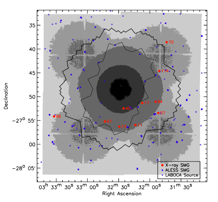
Figure 1.— Full-band X-ray sensitivity map for the E-CDF-S region. The gray-scale levels, from black to light gray, represent areas with flux limits of $<4.0\times 10^{-17}$, $4.0\times 10^{-17}$ to $10^{-16}$, $10^{-16}$ to $3.3\times 10^{-16}$, $3.3\times 10^{-16}$ to $10^{-15}$, and $>10^{-15}$ erg cm^-2 s^-1, respectively. For the overlapping region of the CDF-S and E-CDF-S where each sensitivity map reports a different flux limit, the smaller one (representing the best sensitivity) was used when creating the merged sensitivity map. The large red dots mark the X-ray detected SMGs, while the blue dots are other SMGs in the ALESS main catalog. X-ray detected SMGs are labeled with their short LESS IDs (e.g., ALESS 11.1 is labeled as “11”). The same labeling convention also applies to all plots following. The small open circles are the LABOCA submm sources (Weiß et al., 2009) that were followed up by ALMA but whose fields do not contain any ALESS main-catalog source (57 such sources; see Hodge et al. 2013 for details). The inner thin solid line shows the GOODS-S region (Giavalisco et al., 2004), which is also approximately the combined coverage for Hubble WFC3 Early Release Science and CANDELS (Grogin et al., 2011) in this region. The outer thick solid line marks the region for the 4 Ms CDF-S (X11). The LABOCA region is roughly a square whose edges are $\sim$ 2–3$\arcmin$ outside the E-CDF-S boundaries. The average exposure time of the X-ray detected SMGs is 2.2 Ms, while for the X-ray undetected SMGs it is 0.8 Ms. As also discussed in Section 5, some of the non-detections are simply due to shallower X-ray coverage.

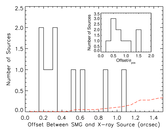
Figure 2.— Histogram of the positional offsets between the SMGs and their X-ray counterparts. The red dashed line is the average number of expected false matches, estimated for the search radius shown on the $x$-axis. For a matching radius of $1.5\arcsec$, the expected number of false match is 0.3 (consistent with the estimate given the likelihood-ratio method). The inset plot shows the histogram of offset$/\sigma_{\rm pos}$, where $\sigma_{\rm pos}$ is the quadrature sum of the positional error of each SMG and that of its matched X-ray source. None of our sources has an offset of over 2$\sigma_{\rm pos}$. See Section 2.3 for details.

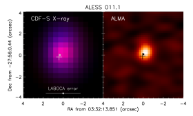
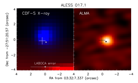
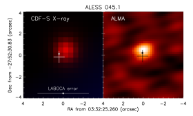
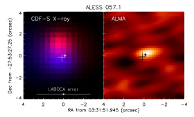
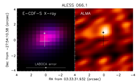
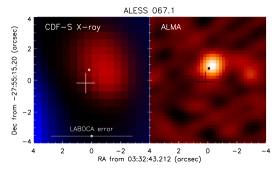
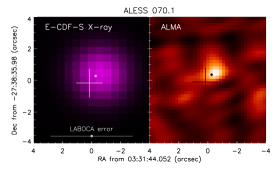
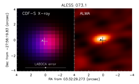
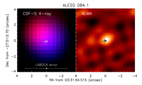
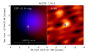
Figure 3.— X-ray and submm images of the X-ray detected SMGs (central R.A. and Dec. given in the $x$- and $y$-axis labels). The title gives the ALESS short ID for each source. The dot (with a plus sign) marks the submm position and the larger plus sign marks the X-ray position, with the sizes being their respective $\pm 1\sigma$ positional errors. Most of the submm positional error bars are too small to see ($<0.1\arcsec$). The LABOCA $1\sigma$ positional error bar is illustrated near the bottom of each X-ray image panel. The X-ray image (smoothed) is color-coded so that the 0.5–2 keV soft band image is red, while the 2–8 keV hard band image is blue. For sources at large off-axis angles, the X-ray positions are determined with a matched-filter technique to account for the complex PSFs (for sources at $>8\arcmin$ in the CDF-S and $>6\arcmin$ in the E-CDF-S; see L05 and X11 for details). Therefore, for sources at large off-axis angles, the position may appear shifted from the centroid of the smoothed image. The submm images are from Hodge et al. (2013) and Karim et al. (2013); X-ray images are from X11; and LABOCA positional errors are from Biggs et al. (2011).

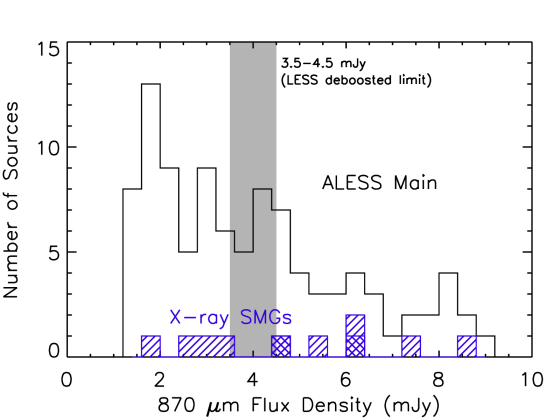
Figure 4.— Histograms of the 870 $\mu$m flux density for the ALESS main-catalog sources (solid line) and for the X-ray detected SMGs (hatched). The two sources plotted in cross-hatched histogram are ALESS 45.1 and 67.1, which are not classified as AGNs in Section 4. The gray region marks the deboosted flux limit of the LESS survey, whose submm sensitivity is about a factor of three poorer than that of ALESS (Weiß et al., 2009). The flux distribution of all ALESS SMGs does not appear statistically different from that of the X-ray detected SMGs, consistent with the result of a K-S test ($p=0.39$; see Section 2.3).

Figure 5.— X-ray spectral fits for ALESS 11.1, 57.1, 66.1, 84.1, and 114.2. Below the panel title the 0.5–8.0 keV (full-band) net photon counts and full-band effective exposure time are given, as also listed in Table 2. The solid lines in the upper panels of each sub-plot are the best-fit models (a power-law with the effects of both Galactic and intrinsic absorption, XSPEC wabs*zwabs*zpow), except for ALESS 66.1 in sub-plot (c), whose best-fit model has no intrinsic absorption (wabs*zpow). The upper $x$-axis gives the energy in the source rest frame. The lower panel in each sub-plot shows the ratio between the data and the best-fit model. The inset figures are the contours for the intrinsic photon index $\Gamma_{\rm int}$ and column density $N_{\rm H}$ at the 68.3%, 90%, and 99% confidence levels. The diamonds mark the best-fit values. The $\Gamma_{\rm int}$-$N_{\rm H}$ contours for ALESS 66.1 were computed using a wabs*zwabs*zpow model (different from its best-fit model wabs*zpow), which demonstrates that this source shows no detectable absorption. See Section 3.2 for more details.

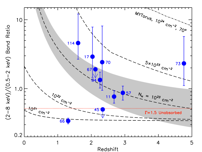
Figure 6.— The hardness ratio between the 2–8 keV (hard) and 0.5–2 keV (soft) bands (i.e., X-ray hardness) vs. redshift for our SMGs. Plotted are 1$\sigma$ error bars (68.3% CIs) for the hardness ratios. See the notes in Table 2 and Section 3.2 for details on the hardness ratios and their error bars (or 90% CI upper limits for ALESS 45.1 and 67.1). The dashed lines are tracks for AGN spectral models described by a power-law with the effects of both Galactic and intrinsic absorption with the intrinsic photon index $\Gamma_{\rm int}$ fixed to 1.8 (XSPEC wabs*zwabs*zpow). The shaded region is for models with a varying $\Gamma_{\rm int}=1.8\pm 0.5$ for $N_{\rm H}=10^{23}$ cm^-2. The dash dotted lines are tracks calculated using the MYTorus model (Murphy & Yaqoob 2009), with $\Gamma=1.8$, $N_{\rm H}=10^{24}$ cm^-2, and inclination angles of $50^{\circ}$ and $70^{\circ}$. The red dotted line marks the expected hardness ratio for $\Gamma=1.5$ and no intrinsic absorption, which could also describe a typical starbust/HMXB population (e.g., Teng et al. 2005; Lehmer et al. 2008). See Section 3.2 for additional discussion.

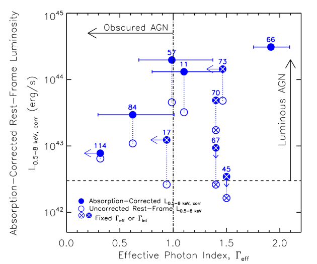
Figure 7.— Classification Method I & II: Sources with observed effective photon index ($x$-axis) $\Gamma_{\rm eff}<1.0$ (to the left of the dash-dotted line) are classified as obscured AGNs (Method I in Table 1), and sources with rest-frame 0.5–8.0 keV absorption-corrected luminosity ($y$-axis, filled circles) $L_{\rm 0.5-8\ keV,corr}>3\times 10^{42}$ erg s^-1 (above the dashed line) are classified as luminous AGNs (Method II; see Section 4.1). The open circles connected to each source by a dotted line are the rest-frame 0.5–8.0 keV apparent luminosity $L_{\rm 0.5-8\ keV}$ (without intrinsic absorption correction). Error bars along the $x$-axis direction mark the 90% confidence intervals for $\Gamma_{\rm eff}$; arrows indicate 90% upper limits (see the notes in Table 2 and Section 3.2 for details). The $\Gamma_{\rm eff}$ of ALESS 45.1 is plotted at 1.5 only for display clarity. Crosses mark the $L_{\rm 0.5-8\ keV}$ (or $L_{\rm 0.5-8\ keV,corr}$) values with larger uncertainties due to fixed $\Gamma_{\rm eff}$ (or $\Gamma_{\rm int}$) as a result of having low counts. These two classification criteria do not rule out ALESS 45.1, 67.1 or 70.1 as being AGNs, but to be conservative, we do not classify them as AGNs here (see Table 1). See Section 4.1 for more details.

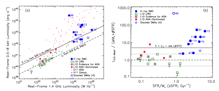
Figure 8.— Classification Method III: Panel (a): The rest-frame 0.5–8.0 keV apparent luminosity (no absorption correction) vs. the rest-frame 1.4 GHz monochromatic luminosity. The dashed line marks the $L_{\rm 0.5-8\ keV}$ to $L_{\rm 1.4\ GHz}$ ratio as calculated by converting $L_{\rm 1.4\ GHz}$ into star formation rate (SFR) following PR07, and then converting SFR into $L_{\rm 0.5-8\ keV}$ following L10. Panel (b): The ratio between the rest-frame 0.5–8.0 keV apparent luminosity $L_{\rm 0.5-8\ keV}$ and the expected 0.5–8.0 keV luminosity from star formation (calculated following L10) vs. the specific Star-Formation Rate (sSFR; $SFR/M_{\star}$, in per billion years, Gyr^-1). The dashed line marks the best-fit correlation of $L_{\rm 0.5-8\ keV}=\alpha M_{\star}+\beta\mbox{SFR}$ in L10, and the dotted lines show the 1$\sigma$ scatter in this correlation. For both panels: SMGs above the solid line (having $L_{\rm 0.5-8\ keV}>5\times L_{\rm X,SF}$) are classified as AGN hosts. As in previous plots, X-ray detected SMGs are plotted as large blue dots and labeled with their short LESS IDs. ALESS 66.1 is plotted as an open circle here as its stellar-mass estimate has high uncertainty (see Section 4.2). For comparison, the sources from L10 are also plotted. The green squares are LIRGs from L10, red dots are L10 LIRGs that are dominated by AGNs in the X-ray, and green squares with red dots in the center represent L10 LIRGs which show evidence of AGN activity. The small red dots are X-ray sources classified as ‘AGNs’ by X11, and the small green squares are sources classified as ‘Galaxies’ by X11. The star marks the average radio luminosity and averaged stacked X-ray luminosity for the 4 radio-bright SMGs in our stacking sample (see Section 6). All SMGs other than ALESS 17.1, 45.1, and 67.1 are classified as AGN hosts under Method III. See Section 4.2 and the notes in Table 4 for more details.

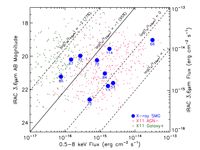
Figure 9.— Classification Method IV: IRAC 3.6 $\mu$m magnitude/flux vs. observed-frame 0.5–8.0 keV flux $f_{\rm 0.5-8\ keV}$ (with no absorption correction). The small red dots and green squares are for the X-ray sources in X11. However, as detailed in Section 4.3, to be conservative, the sources that have $z>1$ and were classified as ‘AGNs’ only under the $f_{R}$–$f_{\rm 0.5-8\ keV}$ criterion in X11 were taken as ‘Galaxies’ here (hence the label ‘AGN$-$’ and ‘Galaxy$+$’). To the lower right of the solid line ($\log{(f_{\rm 0.5-8\ keV}/f_{\rm 3.6\mu m})}>-1$), 95% of the X11 sources on the plot are AGNs (similarly for the 77% label). Therefore, we choose to classify the SMGs with $\log(f_{\rm 0.5-8\ keV}/f_{\rm 3.6\mu m})>-1$ as AGNs. For X11 sources that are only detected in the soft band or the hard band, the corresponding fluxes in the detection band are used instead of full-band flux upper limits.

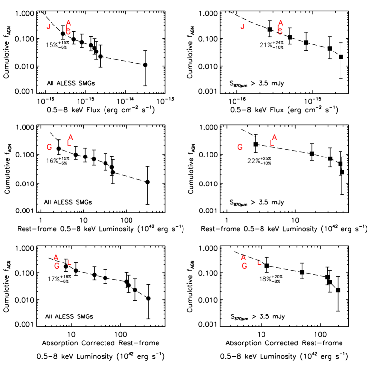
Figure 10.— Cumulative AGN fraction $f_{\rm AGN}$ for SMGs as a function of the observed-frame 0.5–8.0 keV flux ($f_{\rm 0.5-8\ keV}$), rest-frame 0.5–8.0 keV apparent luminosity ($L_{\rm 0.5-8\ keV}$), or rest-frame 0.5–8.0 keV absorption-corrected luminosity ($L_{\rm 0.5-8\ keV,corr}$). Each point represents the AGN fraction in the SMG sample for AGNs with a certain X-ray flux/luminosity value or larger. The percentage number and error bars given are for the left-most point on each plot (also listed in Table 5). The plotted flux or luminosity values are those of the 8 SMG-AGNs, as listed in Tables 1 and 2. The dashed lines are the $f_{\rm AGN}$ results if we classify all 10 X-ray SMGs (i.e., including ALESS 45.1 and 67.1) as AGNs. The three panels on the left (with filled circles) show $f_{\rm AGN}$ calculated using all ALESS main-catalog sources, while the three on the right (with filled squares) show $f_{\rm AGN}$ calculated using only ALESS sources that have $S_{\rm 870\mu\mbox{m}}>3.5$ mJy (a flux-limited sample; see Section 5.1). Error bars are 1$\sigma$ errors calculated using the methods in Gehrels (1986). The red letters mark the $f_{\rm AGN}$ estimates by Alexander et al. (2005b; ‘A’), Laird et al. (2010; ‘L’), Georgantopoulos et al. (2011; ‘G’), and Johnson et al. (2013; ‘J’, lowest X-ray luminosity values are not available thus not plotted in the four lower panels). See Section 5 and Section 7.1.1 for more details.

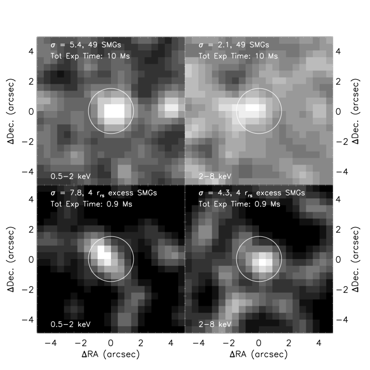
Figure 11.— Stacked X-ray images (Gaussian smoothed with a FWHM of 3 pixels) for the 49 SMGs within $7\arcmin$ of any of the E-CDF-S aim points (top) and for the 4 SMGs with $r_{\rm rs}$ excesses (bottom). On the left are the stacked images in the soft band (0.5–2 keV), and on the right are the hard band (2–8 keV). The circles show the size of the extraction aperture ($1.5\arcsec$ radius) for the source, which is the same for the individual background region (1000 such background regions were used to estimate the mean background for each band). See Section 6 for details.

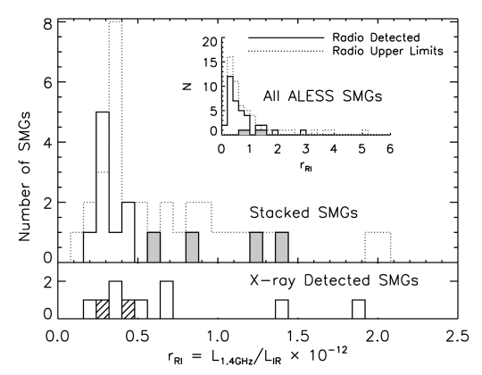
Figure 12.— Histogram of the ratios between the rest-frame 1.4 GHz monochromatic luminosity, $L_{\rm 1.4GHz}$, and the rest-frame IR luminosity, $L_{\rm IR}$ (8–1000 $\mu$m). The inset is for all ALESS SMGs and the lower panel for the 10 X-ray detected ones (non-AGN in hatched marks). Overall, the SMG-AGNs have high $r_{\rm RI}$ values, especially considering that the majority of SMGs only have radio upper limits but not detections (dotted histograms). Just like the X-ray detected SMGs, the four sources that are selected as potential AGN candidates in the stacking analysis (shaded in gray) are high in $r_{\rm RI}$ compared to either the rest of SMGs in the stacking sample or all ALESS SMGs. See Section 6 for details.

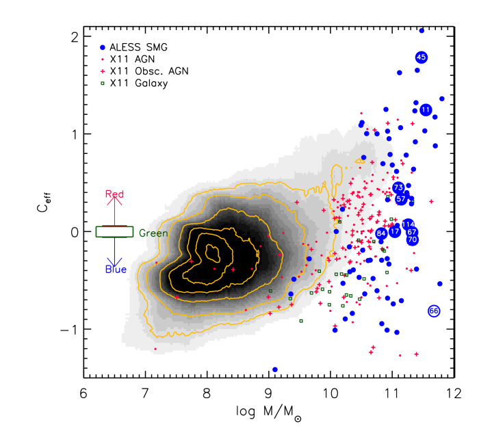
Figure 13.— Effective color vs. stellar mass. The effective color is defined as $C_{\rm eff}=(U-V)_{\rm rest}+0.31z+0.08M_{V}+0.51$, as in Bell et al. (2004). The divisions defined by $C_{\rm eff}$ values for the red sequence, blue cloud, and green valley are illustrated on the left side by the red/blue arrows and green square. The grayscale density map and contours (levels for 0.5, 1–5 sources per pixel) are for $\sim 20,000$ galaxies with $1\leqslant z\leqslant 5$ (a similar redshift range as for the ALESS SMGs) within the GOODS-S region. The galaxies are from the $z$-band selected catalog of Dahlen et al. (2010), with their $C_{\rm eff}$ values and stellar masses calculated by Xue et al. (2012). The red dots and crosses are the X11 AGNs, and green squares mark the X11 galaxies (both with $1\leqslant z\leqslant 5$). The red crosses are AGNs that are classified as obscured AGN by X11 as they have $\Gamma_{\rm eff}<1$. Other symbols are the same as in previous figures: blue dots for SMGs, with larger dots for the X-ray detected SMGs, labeled with their short LESS IDs. Again ALESS 66.1 is plotted as an open circle as its stellar mass has large uncertainty (see Section 3.3). See Section 7.2.1 for more discussion.

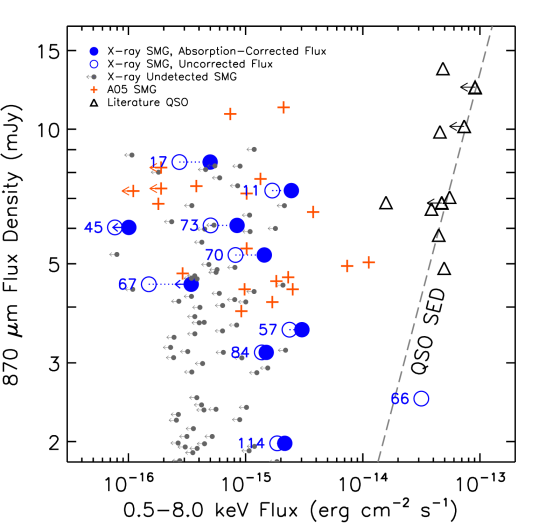
Figure 14.— Observed 870 $\mu$m flux density vs. 0.5–8.0 keV flux for our X-ray detected SMGs (large open blue circles), the X-ray detected SMGs in A05 (orange crosses), and quasars from the literature (black triangles). The large blue dots connected with dotted lines are for the absorption-corrected 0.5–8.0 keV flux (observed frame). The dots labeled with leftward arrows indicate 90% confidence upper limits as the hardness ratios for ALESS 45.1 and 67.1 are not well constrained and are given as 90% confidence upper limits (see Section 3.2 and Table 2). The small gray dots with leftward arrows are the X-ray-undetected SMGs with their X-ray flux upper limits (being the 0.5–8.0 keV X-ray sensitivity for their positions in the E-CDF-S region). The dashed line marks the 870 $\mu$m flux density to X-ray flux ratio for a typical 3C273-like unobscured quasar (Fabian et al. 2000). Arrows on the triangles indicate sources with X-ray flux upper limits. The data for the quasars are from Page et al. (2001), Vignali et al. (2001), and Isaak et al. (2002) as also plotted in A05. The $S_{870\mu\mbox{m}}$ of the A05 sources are converted from their $S_{850\mu\mbox{m}}$ values with an assumed submm spectral index of $\alpha=3$ ($S\propto\nu^{\alpha}$; see, e.g., Carilli & Yun 2000), and similarly for the quasars with $\alpha=1$. Except for ALESS 66.1, all of the X-ray detected SMGs show significant 870 $\mu$m flux excesses compared with typical unobscured quasars, indicating that their submm emission is likely host dominated. We remind the reader here that the flux distributions of the X-ray detected SMGs and the rest are not statistically different, as mentioned in the caption of Figure 4. See Section 7.2.2 for more discussion.

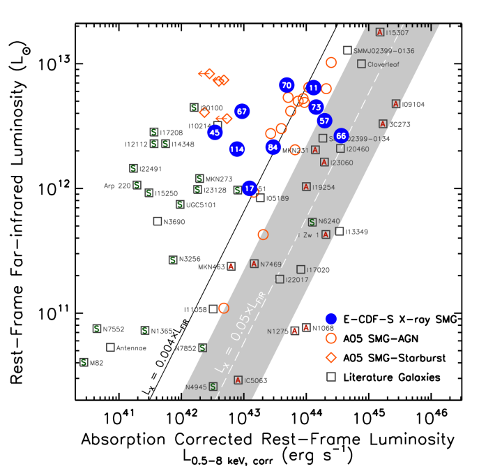
Figure 15.— Rest-frame far-infrared luminosity ($L_{\rm FIR}$) vs. rest-frame 0.5–8.0 keV absorption-corrected luminosity ($L_{\rm 0.5-8\ keV,corr}$). The large blue dots mark the X-ray detected SMGs in this work with their short LESS IDs in the middle. The small orange open circles (diamonds) are for SMG-AGN (SMG-Starbursts) in A05. The open squares are galaxies whose X-ray and far-IR luminosities were calculated by A05 based on data compiled from the literature (see caption of Fig. 8 in A05 and references therein). They are classified either as AGN-dominated (labeled with red letter ‘A’) or star formation-dominated (labeled with green letter ‘S’) by Rigopoulou et al. (1999) and Tran et al. (2001). The dashed line and gray region is the median luminosity ratio for the quasars in Elvis et al. (1994) and its standard deviation. See Section 7.2.2 for more discussion.

Table 1Properties of Matched Submm and X-ray Sources

		$S_{870\mu{\rm m}}$	X-ray Position		CDF-S	E-CDF-S	$f_{X}/10^{-15}$
ALESS SMG Full Name	ID	(mJy)	$\alpha_{\rm J2000.0}$	$\delta_{\rm J2000.0}$	Cat & ID	Cat & ID	erg cm-2 s-1
ALESS J$033213.85-275600.3$	011.1	$7.3\pm 0.4$	03 32 13.85	$-27$ 56 00.44	M 197	M 332	1.69
ALESS J$033207.30-275120.8$	017.1	$8.4\pm 0.5$	03 32 07.34	$-27$ 51 20.57	M 131	$\cdots$	0.27
ALESS J$033225.26-275230.5$	045.1	$6.0\pm 0.5$	03 32 25.26	$-27$ 52 30.83	M 348	$\cdots$	0.08
ALESS J$033151.92-275327.1$	057.1	$3.6\pm 0.6$	03 31 51.95	$-27$ 53 27.25	M 34	M 203	2.37
ALESS J$033331.93-275409.5$	066.1	$2.5\pm 0.5$	03 33 31.93	$-27$ 54 10.58	$\cdots$	M 725	31.60
ALESS J$033243.20-275514.3$	067.1	$4.5\pm 0.4$	03 32 43.21	$-27$ 55 15.20	A	$\cdots$	0.15
ALESS J$033144.02-273835.5$	070.1	$5.2\pm 0.5$	03 31 44.05	$-27$ 38 35.98	$\cdots$	M 146	0.82
ALESS J$033229.29-275619.7$	073.1	$6.1\pm 0.5$	03 32 29.27	$-27$ 56 19.83	M 403	$\cdots$	0.50
ALESS J$033154.50-275105.6$	084.1	$3.2\pm 0.6$	03 31 54.52	$-27$ 51 05.70	M 48	$\cdots$	1.38
ALESS J$033151.11-274437.3$	114.2	$2.0\pm 0.5$	03 31 51.11	$-27$ 44 37.48	M 31	M 194	1.86

Table 2X-ray Properties of X-ray Detected SMGs

ALESS		X-ray	Off-Axis	Exp.	FB	Bkg	Rest-frame	Hardness		$\log{L_{\rm 0.5-8keV}}$		$N_{\rm H}/10^{22}$	$\log{L_{\rm 0.5-8keV,corr}}$
ID	$z$	Cat & ID	Angle	Time	Counts	Counts	Energy (keV)	Ratio	$\Gamma_{\rm eff}$	$\mbox{erg\ s}^{-1}$	$\Gamma_{\rm int}$	cm-2	$\mbox{erg\ s}^{-1}$
011.1	2.6791	CDF-S M 197	$8.2\arcmin$	2.16 Ms	265	297	$1.84$–$29.43$	$0.77^{+0.17}_{-0.15}$	$1.10^{+0.36}_{-0.30}$	43.5	$1.89^{+0.64}_{-0.56}$	$22.4^{+11.4}_{-12.4}$	44.1
017.1	2.0351	CDF-S M 131	$5.4\arcmin$	3.04 Ms	46	83	$1.52$–$24.28$	$2.91^{+4.92}_{-1.46}$	$<0.94$	42.4	(1.80)	25.7	43.1
045.1	$2.34^{+0.26}_{-0.67}$2	CDF-S M 348	$4.1\arcmin$	3.36 Ms	21	37	$1.67$–$26.72$	$<0.86$	(1.40)	42.2	(1.80)	$<6.6$	$<42.5$
057.1	2.9403	CDF-S M 34	$9.4\arcmin$	1.44 Ms	237	306	$1.97$–$31.52$	$0.87^{+0.22}_{-0.19}$	$0.99^{+0.38}_{-0.31}$	43.7	$1.88^{+0.78}_{-0.61}$	$24.7^{+19.7}_{-13.7}$	44.3
066.1	1.3101	E-CDF-S M 725	$7.1\arcmin$	208 ks	676	53	$1.15$–$18.48$	$0.34^{+0.03}_{-0.03}$	$1.92^{+0.18}_{-0.16}$	44.5	$2.03^{+0.11}_{-0.14}$	$<0.2$	$<44.6$
067.1	2.1221	CDF-S A	$7.6\arcmin$	3.05 Ms	38	310	$1.56$–$24.98$	$<6.51$	(1.40)	42.4	(1.80)	$<56.7$	$<43.0$
070.1	2.3251	E-CDF-S M 146	$3.5\arcmin$	222 ks	15	7	$1.66$–$26.60$	$2.42^{+5.69}_{-1.48}$	(1.40)	43.2	(1.80)	27.8	43.7
073.1	4.7624	CDF-S M 403	$7.9\arcmin$	2.85 Ms	82	321	$2.88$–$46.10$	$2.32^{+3.38}_{-1.21}$	$<1.46$	43.7	(1.80)	85.4	44.2
084.1	2.2591	CDF-S M 48	$7.9\arcmin$	2.88 Ms	224	89	$1.63$–$26.07$	$1.34^{+0.40}_{-0.32}$	$0.62^{+0.39}_{-0.33}$	43.0	$1.39^{+1.56}_{-0.84}$	$17.1^{+44.4}_{-15.1}$	43.5
114.2	1.6061	CDF-S M 31	$9.0\arcmin$	1.46 Ms	126	310	$1.30$–$20.85$	$4.59^{+7.53}_{-1.92}$	$<0.32$	42.8	$0.35^{+0.93}_{-0.78}$	$4.8^{+14.7}_{-4.8}$	42.9

Table 3Multiwavelength Properties and Classification of X-ray Detected SMGs

ALESS	$3.6\mu$m	$\log{L_{\rm IR}}$	$\log{L_{\rm FIR}}$	$\log{L_{\rm 1.4GHz}}$	${M_{\star}}$	SFR	Classification					Has
ID	AB mag	${L_{\odot}}$	${L_{\odot}}$	${\rm W\ Hz^{-1}}$	$10^{11}\ {M_{\odot}}$	$M_{\odot}$yr-1	I	II	III	IV	V	AGN?
011.1	21.8	$12.90^{+0.12}_{-0.04}$	$12.81^{+0.12}_{-0.04}$	24.42	$3.5\pm 1.3$	$1420^{+340}_{-130}$	N	Y	Y	Y	N	Y
017.1	20.0	$12.21^{+0.03}_{-0.11}$	$12.00^{+0.03}_{-0.13}$	24.48	$1.1\pm 0.5$	$290^{+20}_{-80}$	Y	N	N	N	N	Y
045.1	21.2	$12.55^{+0.07}_{-0.02}$	$12.45^{+0.07}_{-0.02}$	24.03	$3.0\pm 1.1$	$630^{+90}_{-40}$	N	N	N	N	N	?
057.1	21.6	$12.64^{+0.08}_{-0.07}$	$12.54^{+0.08}_{-0.08}$	24.46	$1.4\pm 1.0$	$790^{+130}_{-140}$	Y	Y	Y	Y	N	Y
066.1	19.0	$12.51^{+0.10}_{-0.06}$	$12.42^{+0.11}_{-0.06}$	23.77	$4.8\pm 3.4$	$580^{+120}_{-80}$	N	Y	Y	Y	N	Y
067.1	20.2	$12.72^{+0.12}_{-0.06}$	$12.62^{+0.12}_{-0.06}$	24.40	$2.1\pm 1.5$	$950^{+230}_{-130}$	N	N	N	N	N	?
070.1	20.2	$12.90^{+0.07}_{-0.04}$	$12.83^{+0.07}_{-0.05}$	25.04	$2.1\pm 1.5$	$1420^{+220}_{-150}$	N	N	Y	Y	N	Y
073.1	22.6	$12.75^{+0.09}_{-0.12}$	$12.65^{+0.09}_{-0.14}$	24.51	$1.3\pm 0.3$	$1000^{+190}_{-320}$	N	Y	Y	Y	N	Y
084.1	21.0	$12.43^{+0.13}_{-0.05}$	$12.33^{+0.14}_{-0.05}$	24.03	$0.7\pm 0.5$	$480^{+130}_{-60}$	Y	Y	Y	Y	Y	Y
114.2	19.6	$12.42^{+0.05}_{-0.14}$	$12.32^{+0.05}_{-0.15}$	24.14	$1.8\pm 0.6$	$470^{+50}_{-190}$	Y	Y	Y	Y	N	Y

Table 4Classification Methods

Method	Relevant Figure	Classified as AGN if …	Reference
I	7	$\Gamma_{\rm eff}<1.0$	Alexander et al. (2005b); Xue et al. (2011)
II	7	$L_{\rm 0.5-8\ keV,corr}>3\times 10^{42}$ erg s-1	Bauer et al. (2004); Lehmer et al. (2008); Xue et al. (2011)
IIIa	8a	$L_{\rm 0.5-8\ keV}>5\times L_{\rm 0.5-8\ keV}$ as	Persic & Rephaeli (2007); Lehmer et al. (2010);
		expected from $L_{\rm 1.4\ GHz}$ (SFR)	Alexander et al. (2005b); Xue et al. (2011)
IIIb	8b	$L_{\rm 0.5-8\ keV}>5\times(L_{\rm 0.5-8\ keV}=\alpha M_{\star}+\beta$SFR$)$	Lehmer et al. (2010)
IV	9	$\log{(f_{\rm X}/f_{\rm 3.6\mu m})}>-1$	This paper — see Section 4.3
V	$\cdots$	X-ray Variable	Young et al. (2012)

Table 5AGN Fractions

	$f_{\rm X}>f_{\rm X,min}$	$L_{\rm X}>L_{\rm X,min}$	$L_{\rm X,corr}>L_{\rm X,corr,min}$
All ALESS $f_{\rm AGN}$ (%)	$14.9^{+14.8}_{-5.5}$	$15.5^{+15.3}_{-5.7}$	$17.0^{+15.9}_{-5.9}$
$S_{\rm 870\mu m}>3.5$ mJy $f_{\rm AGN}$	$21.0^{+23.7}_{-9.5}$	$21.6^{+24.9}_{-10.2}$	$18.1^{+20.1}_{-7.7}$

Table 6Stacking Results

Stacking	Number	Full-Band		Hardness		Mean Full-Band Flux	Median	Mean Rest-Frame Luminosity
Sample	of SMGs	Net Counts	S/N	Ratio	$\Gamma_{\rm eff}$	$f_{\rm 0.5-8\ keV}$ (erg cm-2 s-1)	Redshift	$L_{\rm 0.5-8\ keV}$ (erg s-1)
All	49	$33.2^{+10.5}_{-9.5}$	$4.5\sigma$	$0.6^{+0.6}_{-0.4}$	$1.3^{+1.2}_{-0.6}$	$5.5\times 10^{-17}$	2.6	$1.2\times 10^{42}$
$r_{\rm RI}\geqslant 0.5$	4	$15.5^{+5.6}_{-4.4}$	$7.4\sigma$	$1.0^{+0.8}_{-0.5}$	$0.8^{+0.6}_{-0.5}$	$3.6\times 10^{-16}$	2.2	$3.6\times 10^{42}$
$r_{\rm RI}<0.5$	45	$17.7^{+9.4}_{-8.4}$	$2.5\sigma$	$0.4^{+0.8}_{-0.4}$	$1.6^{+2.3}_{-1.0}$	$2.7\times 10^{-17}$	2.9	$1.2\times 10^{42}$

References

- Aird et al. (2012) Aird, J., et al. 2012, ApJ, 746, 90
- Alexander et al. (2003) Alexander, D. M., et al. 2003, AJ, 126, 539
- Alexander et al. (2005a) Alexander, D. M., Smail, I., Bauer, F. E., Chapman, S. C., Blain, A. W., Brandt, W. N., & Ivison, R. J. 2005, Nature, 434, 738
- Alexander et al. (2005b) Alexander, D. M., Bauer, F. E., Chapman, S. C., Smail, I., Blain, A. W., Brandt, W. N., & Ivison, R. J. 2005, ApJ, 632, 736 (A05)
- Alonso-Herrero (2013) Alonso-Herrero, A. 2013, arXiv:1302.2033
- Aretxaga et al. (2007) Aretxaga, I., et al. 2007, MNRAS, 379, 1571
- Arnaud (1996) Arnaud, K. A. 1996, Astronomical Data Analysis Software and Systems V, 101, 17
- Austermann et al. (2010) Austermann, J. E., et al. 2010, MNRAS, 401, 160
- Barger et al. (1998) Barger, A. J., Cowie, L. L., Sanders, D. B., Fulton, E., Taniguchi, Y., Sato, Y., Kawara, K., & Okuda, H. 1998, Nature, 394, 248
- Barger et al. (2012) Barger, A. J., Wang, W.-H., Cowie, L. L., Owen, F. N., Chen, C.-C., & Williams, J. P. 2012, ApJ, 761, 89
- Basu-Zych et al. (2013) Basu-Zych, A. R., et al. 2013, ApJ, 762, 45
- Bauer et al. (2004) Bauer, F. E., Alexander, D. M., Brandt, W. N., Schneider, D. P., Treister, E., Hornschemeier, A. E., & Garmire, G. P. 2004, AJ, 128, 2048
- Bell et al. (2004) Bell, E. F., et al. 2004, ApJ, 608, 752
- Bielby et al. (2012) Bielby, R. M., Hill, M. D., Metcalfe, N., & Shanks, T. 2012, MNRAS, 419, 1315
- Biggs et al. (2011) Biggs, A. D., et al. 2011, MNRAS, 413, 2314
- Bolzonella et al. (2000) Bolzonella, M., Miralles, J.-M., & Pelló, R. 2000, A&A, 363, 476
- Borys et al. (2004) Borys, C., Scott, D., Chapman, S., Halpern, M., Nandra, K., & Pope, A. 2004, MNRAS, 355, 485
- Borys et al. (2005) Borys, C., Smail, I., Chapman, S. C., Blain, A. W., Alexander, D. M., & Ivison, R. J. 2005, ApJ, 635, 853
- Bothwell et al. (2013) Bothwell, M. S., et al. 2013, MNRAS, 429, 3047
- Bruzual & Charlot (2003) Bruzual, G., & Charlot, S. 2003, MNRAS, 344, 1000
- Broos et al. (2010) Broos, P. S., Townsley, L. K., Feigelson, E. D., Getman, K. V., Bauer, F. E., & Garmire, G. P. 2010, ApJ, 714, 1582
- Carilli & Yun (2000) Carilli, C. L., & Yun, M. S. 2000, ApJ, 530, 618
- Carrera et al. (2013) Carrera, F. J., Ali, A. K., Page, M. J., et al. 2013, arXiv:1302.2844
- Cash (1979) Cash, W. 1979, ApJ, 228, 939
- Chary & Elbaz (2001) Chary, R., & Elbaz, D. 2001, ApJ, 556, 562
- Chapman et al. (2002) Chapman, S. C., Scott, D., Borys, C., & Fahlman, G. G. 2002, MNRAS, 330, 92
- Chapman et al. (2003) Chapman, S. C., Blain, A. W., Ivison, R. J., & Smail, I. R. 2003, Nature, 422, 695
- Chapman et al. (2004) Chapman, S. C., Smail, I., Windhorst, R., Muxlow, T., & Ivison, R. J. 2004, ApJ, 611, 732
- Chapman et al. (2005) Chapman, S. C., Blain, A. W., Smail, I., & Ivison, R. J. 2005, ApJ, 622, 772
- Chen et al. (2013) Chen, C.-T. J., et al. 2013, arXiv:1306.1227
- Ciliegi et al. (2003) Ciliegi, P., Zamorani, G., Hasinger, G., Lehmann, I., Szokoly, G., & Wilson, G. 2003, A&A, 398, 901
- Connolly et al. (1997) Connolly, A. J., Szalay, A. S., Dickinson, M., Subbarao, M. U., & Brunner, R. J. 1997, ApJ, 486, L11
- Coppin et al. (2006) Coppin, K., et al. 2006, MNRAS, 372, 1621
- Coppin et al. (2008) Coppin, K., et al. 2008, MNRAS, 384, 1597
- Coppin et al. (2010) Coppin, K., et al. 2010, ApJ, 713, 503
- Coppin et al. (2012) Coppin, K. E. K., et al. 2012, MNRAS, 427, 520
- Cucciati et al. (2012) Cucciati, O., et al. 2012, A&A, 539, A31
- Daddi et al. (2007) Daddi, E., et al. 2007, ApJ, 670, 156
- Dahlen et al. (2010) Dahlen, T., et al. 2010, ApJ, 724, 425
- Dai et al. (2012) Dai, Y. S., Bergeron, J., Elvis, M., et al. 2012, ApJ, 753, 33
- Damen et al. (2011) Damen, M., et al. 2011, ApJ, 727, 1
- Danielson et al. (in prep.) Danielson, A., et al. 2013, in prep
- Del Moro et al. (2013) Del Moro, A., et al. 2013, A&A, 549, A59
- Donley et al. (2005) Donley, J. L., Rieke, G. H., Rigby, J. R., & Pérez-González, P. G. 2005, ApJ, 634, 169
- Donley et al. (2012) Donley, J. L., et al. 2012, ApJ, 748, 142
- Downes et al. (2012) Downes, T. P., Welch, D., Scott, K. S., Austermann, J., Wilson, G. W., & Yun, M. S. 2012, MNRAS, 423, 529
- Elbaz et al. (2011) Elbaz, D., et al. 2011, A&A, 533, A119
- Elvis et al. (1994) Elvis, M., et al. 1994, ApJS, 95, 1
- Engel et al. (2010) Engel, H., et al. 2010, ApJ, 724, 233
- Feigelson & Babu (2012) Feigelson, E. D., & Babu, J. G. 2012, Modern Statistical Methods for Astronomy, Cambridge, UK: Cambridge University Press
- Feldmann et al. (2006) Feldmann, R., et al. 2006, MNRAS, 372, 565
- Ferrarese & Merritt (2000) Ferrarese, L., & Merritt, D. 2000, ApJ, 539, L9
- Fruscione et al. (2006) Fruscione, A., et al. 2006, Proc. SPIE, 6270,
- Gebhardt et al. (2000) Gebhardt, K., et al. 2000, ApJ, 539, L13
- Georgantopoulos et al. (2011) Georgantopoulos, I., Rovilos, E., & Comastri, A. 2011, A&A, 526, A46 (G11)
- Giavalisco et al. (2004) Giavalisco, M., et al. 2004, ApJ, 600, L93
- Gilli et al. (2011) Gilli, R., et al. 2011, ApJ, 730, L28
- Gilli (2013) Gilli, R. 2013, arXiv:1304.3665
- Grogin et al. (2011) Grogin, N. A., et al. 2011, ApJS, 197, 35
- Gültekin et al. (2009) Gültekin, K., et al. 2009, ApJ, 698, 198
- Häring & Rix (2004) Häring, N., & Rix, H.-W. 2004, ApJ, 604, L89
- Hainline et al. (2011) Hainline, L. J., Blain, A. W., Smail, I., Alexander, D. M., Armus, L., Chapman, S. C., & Ivison, R. J. 2011, ApJ, 740, 96
- Hodge et al. (2013) Hodge, J. A., et al. 2013, ApJ, 768, 91
- Hornschemeier et al. (2001) Hornschemeier, A. E., et al. 2001, ApJ, 554, 742
- Hill & Shanks (2011) Hill, M. D., & Shanks, T. 2011, MNRAS, 410, 762
- Holland et al. (1999) Holland, W. S., et al. 1999, MNRAS, 303, 659
- Hopkins et al. (2007) Hopkins, P. F., Richards, G. T., & Hernquist, L. 2007, ApJ, 654, 731
- Hopkins et al. (2008) Hopkins, P. F., Hernquist, L., Cox, T. J., & Kereš, D. 2008, ApJS, 175, 356
- Hopkins et al. (2010) Hopkins, P. F., Younger, J. D., Hayward, C. C., Narayanan, D., & Hernquist, L. 2010, MNRAS, 402, 1693
- Hughes et al. (1998) Hughes, D. H., et al. 1998, Nature, 394, 241
- Isaak et al. (2002) Isaak, K. G., Priddey, R. S., McMahon, R. G., Omont, A., Peroux, C., Sharp, R. G., & Withington, S. 2002, MNRAS, 329, 149
- Ivison et al. (1998) Ivison, R. J., Smail, I., Le Borgne, J.-F., Blain, A. W., Kneib, J.-P., Bezecourt, J., Kerr, T. H., & Davies, J. K. 1998, MNRAS, 298, 583
- Ivison et al. (2000) Ivison, R. J., Smail, I., Barger, A. J., Kneib, J.-P., Blain, A. W., Owen, F. N., Kerr, T. H., & Cowie, L. L. 2000, MNRAS, 315, 209
- Ivison et al. (2002) Ivison, R. J., et al. 2002, MNRAS, 337, 1
- Iwasawa et al. (2011) Iwasawa, K., et al. 2011, A&A, 529, A106
- Johnson et al. (2013) Johnson, S. P., et al. 2013, MNRAS, 431, 662 (J13)
- Karim et al. (2013) Karim, A., et al. 2013, MNRAS, 432, 2
- Kartaltepe et al. (2012) Kartaltepe, J. S., et al. 2012, ApJ, 757, 23
- Kennicutt (1998) Kennicutt, R. C., Jr. 1998, ApJ, 498, 541
- Komatsu et al. (2011) Komatsu, E., et al. 2011, ApJS, 192, 18
- Koss et al. (2013) Koss, M., Mushotzky, R., Baumgartner, W., Veilleux, S., Tueller, J., Markwardt, C., & Casey, C. M. 2013, ApJ, 765, L26
- Kovács et al. (2006) Kovács, A., Chapman, S. C., Dowell, C. D., Blain, A. W., Ivison, R. J., Smail, I., & Phillips, T. G. 2006, ApJ, 650, 592
- Lacy et al. (2004) Lacy, M., et al. 2004, ApJS, 154, 166
- Lacy et al. (2007) Lacy, M., Petric, A. O., Sajina, A., Canalizo, G., Storrie-Lombardi, L. J., Armus, L., Fadda, D., & Marleau, F. R. 2007, AJ, 133, 186
- Laird et al. (2010) Laird, E. S., Nandra, K., Pope, A., & Scott, D. 2010, MNRAS, 401, 2763 (La10)
- Lehmer et al. (2005) Lehmer, B. D., et al. 2005, ApJS, 161, 21 (L05)
- Lehmer et al. (2007) Lehmer, B. D., et al. 2007, ApJ, 657, 681
- Lehmer et al. (2008) Lehmer, B. D., et al. 2008, ApJ, 681, 1163
- Lehmer et al. (2010) Lehmer, B. D., Alexander, D. M., Bauer, F. E., Brandt, W. N., Goulding, A. D., Jenkins, L. P., Ptak, A., & Roberts, T. P. 2010, ApJ, 724, 559 (L10)
- Lehmer et al. (2012) Lehmer, B. D., et al. 2012, ApJ, 752, 46
- Lilly et al. (1999) Lilly, S. J., Eales, S. A., Gear, W. K. P., Hammer, F., Le Fèvre, O., Crampton, D., Bond, J. R., & Dunne, L. 1999, ApJ, 518, 641
- Lindner et al. (2012) Lindner, R. R., Baker, A. J., Beelen, A., Owen, F. N., & Polletta, M. 2012, ApJ, 757, 3
- Lonsdale et al. (2006) Lonsdale, C. J., Farrah, D., & Smith, H. E. 2006, Astrophysics Update 2, 285
- Luo et al. (2008) Luo, B., et al. 2008, ApJS, 179, 19
- Luo et al. (2010) Luo, B., et al. 2010, ApJS, 187, 560
- Luo et al. (2011) Luo, B., et al. 2011, ApJ, 740, 37
- Lutz et al. (2008) Lutz, D., Sturm, E., Tacconi, L. J., et al. 2008, ApJ, 684, 853
- Lutz et al. (2010) Lutz, D., et al. 2010, ApJ, 712, 1287
- Maccacaro et al. (1988) Maccacaro, T., Gioia, I. M., Wolter, A., Zamorani, G., & Stocke, J. T. 1988, ApJ, 326, 680
- Magnelli et al. (2009) Magnelli, B., Elbaz, D., Chary, R. R., Dickinson, M., Le Borgne, D., Frayer, D. T., & Willmer, C. N. A. 2009, A&A, 496, 57
- Magnelli et al. (2012) Magnelli, B., et al. 2012, A&A, 539, A155
- Menéndez-Delmestre et al. (2007) Menéndez-Delmestre, K., et al. 2007, ApJ, 655, L65
- Menéndez-Delmestre et al. (2009) Menéndez-Delmestre, K., et al. 2009, ApJ, 699, 667
- Merloni (2004) Merloni, A. 2004, MNRAS, 353, 1035
- Miller et al. (2008) Miller, N. A., Fomalont, E. B., Kellermann, K. I., Mainieri, V., Norman, C., Padovani, P., Rosati, P., & Tozzi, P. 2008, ApJS, 179, 114
- Mullaney et al. (2012) Mullaney, J. R., et al. 2012, MNRAS, 419, 95
- Murphy & Yaqoob (2009) Murphy, K. D., & Yaqoob, T. 2009, MNRAS, 397, 1549
- Narayanan et al. (2010) Narayanan, D., Hayward, C. C., Cox, T. J., Hernquist, L., Jonsson, P., Younger, J. D., & Groves, B. 2010, MNRAS, 401, 1613
- Nousek & Shue (1989) Nousek, J. A., & Shue, D. R. 1989, ApJ, 342, 1207
- Pérez-González et al. (2005) Pérez-González, P. G., et al. 2005, ApJ, 630, 82
- Page et al. (2001) Page, M. J., Stevens, J. A., Mittaz, J. P. D., & Carrera, F. J. 2001, Science, 294, 2516
- Park et al. (2006) Park, T., Kashyap, V. L., Siemiginowska, A., van Dyk, D. A., Zezas, A., Heinke, C., & Wargelin, B. J. 2006, ApJ, 652, 610
- Persic & Rephaeli (2007) Persic, M., & Rephaeli, Y. 2007, A&A, 463, 481 (PR07)
- Pope et al. (2006) Pope, A., et al. 2006, MNRAS, 370, 1185
- Pope et al. (2008) Pope, A., et al. 2008, ApJ, 675, 1171
- Preacher & Briggs (2001) Preacher, K. J., & Briggs, N. E. 2011, Calculation for Fisher’s Exact Test: An interactive calculation tool for Fisher’s exact probability test for 2 2 tables, http://quantpsy.org
- Rafferty et al. (2011) Rafferty, D. A., Brandt, W. N., Alexander, D. M., Xue, Y. Q., Bauer, F. E., Lehmer, B. D., Luo, B., & Papovich, C. 2011, ApJ, 742, 3
- Ranalli et al. (2003) Ranalli, P., Comastri, A., & Setti, G. 2003, A&A, 399, 39
- Richards (2000) Richards, E. A. 2000, ApJ, 533, 611
- Rigopoulou et al. (1999) Rigopoulou, D., Spoon, H. W. W., Genzel, R., Lutz, D., Moorwood, A. F. M., & Tran, Q. D. 1999, AJ, 118, 2625
- Rodighiero et al. (2011) Rodighiero, G., Daddi, E., Baronchelli, I., et al. 2011, ApJ, 739, L40
- Rosario et al. (2013) Rosario, D. J., et al. 2013, arXiv:1302.1202
- Roy & Norris (1997) Roy, A. L., & Norris, R. P. 1997, MNRAS, 289, 824
- Sanders & Mirabel (1996) Sanders, D. B., & Mirabel, I. F. 1996, ARA&A, 34, 749
- Santini et al. (2012) Santini, P., et al. 2012, A&A, 540, A109
- Sargent et al. (2012) Sargent, M. T., Béthermin, M., Daddi, E., & Elbaz, D. 2012, ApJ, 747, L31
- Schmitt et al. (2006) Schmitt, H. R., Calzetti, D., Armus, L., Giavalisco, M., Heckman, T. M., Kennicutt, R. C., Jr., Leitherer, C., & Meurer, G. R. 2006, ApJ, 643, 173
- Silverman et al. (2008) Silverman, J. D., et al. 2008, ApJ, 675, 1025
- Simpson et al. (in prep.) Simpson, J. M., et al. in prep.
- Smail et al. (1997) Smail, I., Ivison, R. J., & Blain, A. W. 1997, ApJ, 490, L5
- Smail et al. (2004) Smail, I., Chapman, S. C., Blain, A. W., & Ivison, R. J. 2004, ApJ, 616, 71
- Stark et al. (1992) Stark, A. A., Gammie, C. F., Wilson, R. W., Bally, J., Linke, R. A., Heiles, C., & Hurwitz, M. 1992, ApJS, 79, 77
- Stern et al. (2005) Stern, D., et al. 2005, ApJ, 631, 163
- Swinbank et al. (2010) Swinbank, A. M., et al. 2010, Nature, 464, 733
- Swinbank et al. (in prep.) Swinbank, A. M., et al. 2013, in prep
- Tacconi et al. (2008) Tacconi, L. J., et al. 2008, ApJ, 680, 246
- Teng et al. (2005) Teng, S. H., Wilson, A. S., Veilleux, S., Young, A. J., Sanders, D. B., & Nagar, N. M. 2005, ApJ, 633, 664
- Teng & Veilleux (2010) Teng, S. H., & Veilleux, S. 2010, ApJ, 725, 1848
- Tozzi et al. (2006) Tozzi, P., et al. 2006, A&A, 451, 457
- Tran et al. (2001) Tran, Q. D., et al. 2001, ApJ, 552, 527
- Valiante et al. (2007) Valiante, E., Lutz, D., Sturm, E., Genzel, R., Tacconi, L. J., Lehnert, M. D., & Baker, A. J. 2007, ApJ, 660, 1060
- Vanzella et al. (2008) Vanzella, E., et al. 2008, A&A, 478, 83
- Vignali et al. (2001) Vignali, C., Brandt, W. N., Fan, X., Gunn, J. E., Kaspi, S., Schneider, D. P., & Strauss, M. A. 2001, AJ, 122, 2143
- U et al. (2012) U, V., et al. 2012, ApJS, 203, 9
- Wang et al. (2010) Wang, R., Carilli, C. L., Neri, R., et al. 2010, ApJ, 714, 699
- Wang et al. (2011) Wang, W.-H., Cowie, L. L., Barger, A. J., & Williams, J. P. 2011, ApJ, 726, L18
- Wardlow et al. (2011) Wardlow, J. L., et al. 2011, MNRAS, 415, 1479
- Weiß et al. (2009) Weiß, A., et al. 2009, ApJ, 707, 1201
- Whitaker et al. (2012) Whitaker, K. E., van Dokkum, P. G., Brammer, G., & Franx, M. 2012, ApJ, 754, L29
- Wilson et al. (2008) Wilson, G. W., et al. 2008, MNRAS, 386, 807
- Xue et al. (2010) Xue, Y. Q., et al. 2010, ApJ, 720, 368
- Xue et al. (2011) Xue, Y. Q., et al. 2011, ApJS, 195, 10 (X11)
- Xue et al. (2012) Xue, Y. Q., et al. 2012, ApJ, 758, 129
- Young et al. (2012) Young, M., et al. 2012, ApJ, 748, 124
- Zezas et al. (2001) Zezas, A., Fabbiano, G., Prestwich, A., Murray, S., & Ward, M. 2001, The Central Kiloparsec of Starbursts and AGN: The La Palma Connection, 249, 425
- Zheng et al. (2004) Zheng, W., et al. 2004, ApJS, 155, 73