Haldane Statistics for Fractional Chern Insulators with an Arbitrary Chern number

Abstract

In this paper we provide analytical counting rules for the ground states and the quasiholes of fractional Chern insulators with an arbitrary Chern number. We first construct pseudopotential Hamiltonians for fractional Chern insulators. We achieve this by mapping the lattice problem to the lowest Landau level of a multicomponent continuum quantum Hall system with specially engineered boundary conditions. We then analyze the thin-torus limit of the pseudopotential Hamiltonians, and extract counting rules (generalized Pauli principles, or Haldane statistics) for the degeneracy of its zero modes in each Bloch momentum sector.

I Introduction

As the canonical example of topological order, the fractional quantum Hall (FQH) effect was originally discovered in two-dimensional electron gas subject to a strong perpendicular magnetic field. Tsui et al. (1982); Laughlin (1983) Recently, several groups demonstrated numerically that these strongly-correlated phases also exist in a topological flat band characterized by a non-zero Chern number $C$, even in the absence of a magnetic field. Sheng et al. (2011); Neupert et al. (2011a); Regnault and Bernevig (2011) This discovery of the so-called fractional Chern insulators (FCI) generated enormous interest. Parameswaran et al. (2013); Bergholtz and Liu (2013) Subsequent numerical studies Wang et al. (2011); Neupert et al. (2011b); Bernevig and Regnault (2012a); Wu et al. (2012a); Wang et al. (2012a); Venderbos et al. (2012); Läuchli et al. (2013); Liu et al. (2013a); Kourtis et al. (2012); Kourtis and Daghofer (2013) quickly confirmed the presence of more intricate single-component FQH states in lattice models Haldane (1988); Sun et al. (2011); Tang et al. (2011); Hu et al. (2011), such as the Read-Rezayi series Moore and Read (1991); Read and Rezayi (1999); Bernevig and Regnault (2012a); Wu et al. (2012a); Wang et al. (2012a) and the composite-fermion states Jain (1989); Läuchli et al. (2013); Liu et al. (2013a). Powerful techniques from the study of FQH, including density algebra, Girvin et al. (1986); Parameswaran et al. (2012); Bernevig and Regnault (2012a); Goerbig (2012); Roy (2012); Dobardžić et al. (2013) entanglement spectrum, Li and Haldane (2008); Sterdyniak et al. (2011); Regnault and Bernevig (2011); Wu et al. (2012a) parton construction, Wen (1999); Lu and Ran (2012); McGreevy et al. (2012) and the Hamiltonian theory of composite fermions, Murthy and Shankar (2011, 2012) were introduced to understand the topological ground state of FCI and the nature of its excitations. Wu et al. (2012b); Lee et al. (2013); Liu and Bergholtz (2013); Scaffidi and Möller (2012); Wu et al. (2012c); Zhu et al. (2013); Liu et al. (2013b); Lee and Qi (2013) Possible experimental realizations have also been proposed. Cooper and Dalibard (2013); Yao et al. (2013)

Most of the above progress dealt with a topological band with Chern number $C=1$, which is essentially the same Haldane (1988) as the continuum FQH in a periodic potential Kol and Read (1993); Möller and Cooper (2009); Sørensen et al. (2005). The strongly-correlated physics in a $C>1$ Chern band Wang and Ran (2011); Trescher and Bergholtz (2012); Yang et al. (2012); Wang et al. (2012b); Wu et al. (2013a) turned out much richer than the conventional FQH, due to the interplay between topological order and lattice structure. Barkeshli and Qi (2012); Liu et al. (2012); Sterdyniak et al. (2013); Lu and Ran (2012); Barkeshli et al. (2013) Barkeshli and Qi Barkeshli and Qi (2012) mapped a $C>1$ Chern band to a $C$-component lowest Landau level (LLL) using hybrid Wannier states Qi (2011), and suggested the possibility to realize multicomponent FQH states in a single Chern band. Numerical studies Wang et al. (2012b); Liu et al. (2012); Sterdyniak et al. (2013); Grushin et al. (2012) indeed found clear signature of such states, including the color $\mathrm{SU}(C)$ version of the Halperin Halperin (1983) and the non-Abelian spin-singlet states Ardonne and Schoutens (1999) (NASS), but also identified qualitative deviations from these states, Sterdyniak et al. (2013); Liu et al. (2012) which implies a more complex structure than proposed in Ref. Barkeshli and Qi, 2012. In a previous paper, Wu et al. (2013b) we proposed to understand these new features as the consequences of a special set of boundary conditions associated with the LLL mapping. In the simplest case, this alternative boundary condition can be understood as a color-dependent magnetic flux insertion. We demonstrated that the multicomponent LLL in a new Bloch basis can be seen as a single manifold with constant Berry curvature and Chern number $C$. Using pseudopotential Hamiltonians, we constructed model states for FCI with an arbitrary Chern number, and found high overlaps with the exact ground states. Crucially, our model states correctly capture the anomalous features in the particle entanglement spectrum of the $C>1$ FCI that make our states distinct from the conventional multicomponent FQH states.

In this paper we provide details of the mapping between a Chern band and a multicomponent LLL, and demonstrate the distinctive features of our pseudopotential Hamiltonian due to the new boundary conditions. We construct, in a $C$-component LLL, a momentum-space Bloch basis and a hybrid Wannier basis that mimic the lattice counterparts. Both bases entangle the real space and the internal color space. Using the explicit one-body wave functions for the bases, we derive the representation of the projected density operators in both bases. We define model states as the exact zero modes of the pseudopotential Hamiltonian built from the projected density operators. As we demonstrated in our previous paper Wu et al. (2013b), the Bloch basis is useful for numerical studies as it preserves the full lattice symmetry. The hybrid Wannier basis, on the other hand, facilitates the analysis of the pseudopotential Hamiltonian.

We give a detailed analysis of the simplest bosonic pseudopotential Hamiltonian for the Halperin color-entangled states. We show that the pseudopotential Hamiltonian reduces to almost classical electrostatics in the hybrid Wannier basis, when we take the so-called thin-torus limit Tao and Thouless (1983); Bergholtz and Karlhede (2005); Seidel and Lee (2006); Bergholtz and Karlhede (2006); Seidel and Lee (2007); Bergholtz and Karlhede (2008); Seidel and Yang (2008); Ardonne et al. (2008); Seidel (2008); Bergholtz et al. (2008); Seidel and Yang (2011); Kardell and Karlhede (2011); Nakamura et al. (2012); Bernevig and Regnault (2012b) and carry out truncations motivated by previous numerical results. Sterdyniak et al. (2013); Liu et al. (2012) This enables us to write down the form of its zero modes in this limit. However, in contrast to most well-known FQH states such as Laughlin and Read-Rezayi, a purely classical thin-torus description is not possible. We pinpoint the key difference from the conventional multicomponent FQH due to a subtle twist in the hybrid Wannier states, and detail the procedure to compute the total Bloch momentum of each zero mode. The resulting algorithm correctly predicts the degeneracy of the FCI quasiholes in each lattice momentum sector, without resorting to numerical diagonalization, and can be seen as the extension of the generalized Pauli principle Bernevig and Haldane (2008a, b) to the color-entangled states.

II One-Body States in a Multicomponent Lowest Landau Level

In this section we construct one-body bases in a multicomponent LLL that mimic the Bloch and the Wannier bases in a Chern band with an arbitrary Chern number $C$. We consider a $C$-component (generalized spin) electron moving on a torus with a perpendicular uniform magnetic field. The major difference between our approach and the usual treatment of the multicomponent LLL problem is the adoption of a new set of boundary conditions. This alternative choice entangles together the $C$ components and enables us to construct a single manifold of Bloch states with Chern number $C$. In contrast to the usual picture of multicomponent LLL as $C$ separate manifolds (one for each of the $C$ components) each with unity Chern number, our bases provide a natural foundation for the mapping to a single Chern band with an arbitrary Chern number $C$. The central result of this Section is Eq. (27), the expansion of the electron density operator in the Bloch basis.

II.1 Translations Operators

We consider electrons with $C$ internal (color) degrees of freedom

$$|\sigma\rangle,\quad\sigma\in\mathbb{Z}_{C}.$$ (1)

For simplicity, we work on a rectangular torus spanned by $\mathbf{L}_{x}=L_{x}\hat{x}$ and $\mathbf{L}_{y}=L_{y}\hat{y}$, where $L_{x}$ and $L_{y}$ are the two fundamental cycles of the torus, and $\hat{x}$ and $\hat{y}$ are orthonormal. The torus is pierced by a magnetic field in the $-\hat{e}_{z}$ direction, $\mathbf{B}=\nabla\times\mathbf{A}=B\hat{e}_{z}$ with $B<0$. We denote by $e<0$ the charge of the electron. The magnetic length is $l_{B}=\sqrt{\hbar/(eB)}$. We define the total number of fluxes $N_{\phi}$ penetrating the torus by

$$L_{x}L_{y}=2\pi l_{B}^{2}N_{\phi}.$$ (2)

Here we do not assume $N_{\phi}$ to be an integer as in the original treatment of the Landau level on a toroidal geometry Haldane (1985). As we will see soon, the alternative set of boundary conditions we pick only requires

$$CN_{\phi}\in\mathbb{Z}.$$ (3)

This integer is equal to the dimension of the one-body Hilbert space in the lowest Landau level. We define the magnetic translation operator

$$T(\mathbf{a})=e^{-i\mathbf{a}\cdot\mathbf{K}/\hbar},$$ (4)

where

$$\mathbf{K}=-i\hbar\nabla-e\mathbf{A}(\mathbf{r})+e\mathbf{B}\times\mathbf{r}$$ (5)

is the guiding center momentum. The translation $T(\mathbf{a})$ commutes with the one-body Landau Hamiltonian $H=(-i\hbar\nabla-e\mathbf{A})^{2}/(2m)$ but not with the translation $T(\mathbf{b})$ at a different displacement,

$$T(\mathbf{a})T(\mathbf{b})=T(\mathbf{b})T(\mathbf{a})e^{i\hat{z}\cdot\mathbf{a}\times\mathbf{b}/l_{B}^{2}}.$$ (6)

As argued in the introduction, we need to make contact between the multicomponent Landau level states and the Bloch states in a Chern band. For the latter, we consider a single Bloch band with Chern number $C$ in a tight-binding model on a lattice with $N_{x}\times N_{y}$ unit cells. The band has a total of $N_{x}N_{y}$ one-body states, one at each lattice momentum in the $N_{x}\times N_{y}$ Brillouin zone (BZ). To make contact with this lattice system, we first look in the Landau level for a pair of commuting translation operators that also resolve an $N_{x}\times N_{y}$ BZ. To this end, we tune the magnetic field to match the number of one-body states,

$$CN_{\phi}=N_{x}N_{y},$$ (7)

and we consider the magnetic translations over a fictitious $N_{x}\times N_{y}$ unit cell structure of the continuous torus, namely,

$$T_{x} =T(\mathbf{L}_{x}/N_{x}), T_{y} =T(\mathbf{L}_{y}/N_{y}).$$ (8)

The operator $T_{x}$ (resp. $T_{y}$) has $N_{x}$ (resp. $N_{y}$) different eigenvalues. As opposed to the $C=1$ case, however, for generic $C$ they do not commute due to the $N_{\phi}/(N_{x}N_{y})=1/C$ flux over each fictitious plaquette,

$$T_{x}T_{y}=T_{y}T_{x}e^{i2\pi/C}.$$ (9)

To compensate for this, we define the ‘clock and shift’ operators $Q$ and $P$ over the internal (color) Hilbert space by

$$P|\sigma\rangle =|\sigma+1\text{ (mod $C$)}\rangle, Q|\sigma\rangle =e^{i2\pi\sigma/C}|\sigma\rangle.$$ (10)

Both operators are unitary, and they satisfy

$$PQ=QPe^{-i2\pi/C}.$$ (11)

This leads to a pair of commuting composite operators

$$\widetilde{T}_{x} =T_{x}P, \widetilde{T}_{y} =T_{y}Q.$$ (12)

We will refer to this pair as the ‘color-entangled’ magnetic translation operators. For the (color-neutral) Landau Hamiltonian, both operators are good symmetries, and they resolve an $N_{x}\times N_{y}$ Brillouin zone once we specify the boundary conditions. Notice that in general $[T(\mathbf{L}_{x}),\widetilde{T}_{y}]\neq 0$, $[T(\mathbf{L}_{y}),\widetilde{T}_{x}]\neq 0$. This means that we have to abandon the usual boundaries Haldane (1985) $T(\mathbf{L}_{\alpha})=1$, $\alpha=x,y$. Instead, we adopt the color-entangled generalization $\widetilde{T}_{\alpha}^{N_{\alpha}}=1$, namely,

$$T(\mathbf{L}_{x})P^{N_{x}}=T(\mathbf{L}_{y})Q^{N_{y}}=1.$$ (13)

This alternative set of boundary conditions make it possible to construct two sets of basis states in the one-body Hilbert space with desirable properties spelled below.

II.2 Bloch and Wannier Bases

We define the Bloch states $|\mathbf{k}\rangle$ as the simultaneous eigenstates of $\widetilde{T}_{x}$ and $\widetilde{T}_{y}$ within the LLL,

$$\widetilde{T}_{\alpha}|\mathbf{k}\rangle=e^{-i2\pi k_{\alpha}/N_{\alpha}}|\mathbf{k}\rangle,$$ (14)

with $\mathbf{k}=(k_{x},k_{y})\in\mathbb{Z}^{2}$. The $N_{x}N_{y}$ states within the first Brillouin zone

$$\mathrm{1BZ}=[0~{}..~{}N_{x})\times[0~{}..~{}N_{y})$$ (15)

have distinct eigenvalues under $\widetilde{T}_{\alpha}$, and they constitute the Bloch basis in the $N_{x}N_{y}=CN_{\phi}$-dimensional Hilbert space of the $C$-component LLL.

We now look for the explicit wave function $\langle x,y,\sigma|\mathbf{k}\rangle$ for these basis states. We specialize to the Landau gauge $\mathbf{A}=Bx\hat{y}$. Consider the states $|X,k_{y}\rangle$ with $X,k_{y}\in\mathbb{Z}$ defined by the real- and internal-space wave function

$$\!\!\!\!\langle x,y,\sigma|X,k_{y}\rangle=\frac{1}{(\sqrt{\pi}L_{y}l_{B})^{1/2}}\!\!\sum_{m}^{\mathbb{Z}}\delta_{\sigma,X+mN_{x}}^{\text{mod }C}\\ \exp\Big{\{}\textstyle i2\pi\!\left(\frac{XN_{y}+k_{y}C}{C}+mN_{\phi}\right)\frac{y}{L_{y}}\qquad\qquad\qquad\qquad\\ -\frac{1}{2}\!\left[\frac{x}{l_{B}}-\frac{2\pi l_{B}}{L_{y}}\left(\frac{XN_{y}+k_{y}C}{C}+mN_{\phi}\right)\right]^{2}\Big{\}}.\!\!\!\!$$ (16)

Here $X,k_{y}$ are state labels taking integer values, while $x,y$ are real space coordinates taking continuous values, and $\sigma\in\mathbb{Z}_{C}$ is a discrete coordinate in the internal color space. It is not hard to see that $|X,k_{y}\rangle$ belongs to the lowest Landau level, as the above wave function can be recast in the form $f(x+iy,\sigma)\,e^{-x^{2}/(2l_{B}^{2})}$. Moreover, we find that $|X,k_{y}\rangle$ is periodic in $X$, but with a twist in $k_{y}$:

$$|X+N_{x},k_{y}\rangle =|X,k_{y}\rangle,$$ (17)

$$|X,k_{y}+N_{y}\rangle =|X+C,k_{y}\rangle.$$

These relations are reminiscent of the flow of hybrid Wannier states in a Chern insulator Wu et al. (2012b). Moreover, as we prove in Appendix A, the color-entangled magnetic translations [Eq. (12)] have a representation on $|X,k_{y}\rangle$ similar to the representation of the lattice translations on the hybrid Wannier states, namely,

$$\widetilde{T}_{x}|X,k_{y}\rangle =|X+1,k_{y}\rangle,$$ (18)

$$\widetilde{T}_{y}|X,k_{y}\rangle =e^{-i2\pi k_{y}/N_{y}}|X,k_{y}\rangle.$$

We thus refer to these states as the hybrid Wannier states in the $C$-component LLL. It is easy to see the states with $X\in[0~{}..~{}N_{x})$ and $k_{y}\in[0~{}..~{}N_{y})$ are linearly independent. We emphasize that unless $N_{x}$ is divisible by $C$, these states are not color eigenstates, in contrast to the states studied in Ref. Barkeshli and Qi, 2012.

We want to define the Bloch states in the LLL as a Fourier sum of the hybrid Wannier states,

$$|\mathbf{k}\rangle=|k_{x},k_{y}\rangle=\frac{1}{\sqrt{N_{x}}}\sum_{X}^{N_{x}}e^{i2\pi Xk_{x}/N_{x}}|X,k_{y}\rangle.$$ (19)

From Eqs. (17) and (18), we find that the simultaneous eigenvalue equation in (14) indeed holds. These states are periodic in $k_{x}$, but only quasi-periodic in $k_{y}$,

$$|k_{x}+N_{x},k_{y}\rangle =|k_{x},k_{y}\rangle,$$ (20)

$$|k_{x},k_{y}+N_{y}\rangle =e^{-i2\pi k_{x}C/N_{x}}|k_{x},k_{y}\rangle.$$ (21)

The latter non-periodicity signals the topological obstruction to a periodic smooth gauge due to the non-zero Chern number of a Landau level. 

II.3 Projected Density Operator

The density operator projected to the lowest Landau level plays a central role in the FQH physics, as it is used to define the inter-particle interaction. As we now show, this operator takes a particularly nice form in our Bloch basis.

By definition, the density operator of color $\sigma$ at $\mathbf{r}=(x,y)$ projected to the LLL is given by

$$\rho(\mathbf{r},\sigma)=\sum_{\mathbf{k}_{1}}^{\mathrm{BZ}}\sum_{\mathbf{k}_{2}}^{\mathrm{BZ}}|\mathbf{k}_{1}\rangle\phi^{*}_{\mathbf{k}_{1}}(\mathbf{r},\sigma)\phi_{\mathbf{k}_{2}}(\mathbf{r},\sigma)\langle\mathbf{k}_{2}|,$$ (22)

where $\phi_{\mathbf{k}}(\mathbf{r},\sigma)=\langle\mathbf{r},\sigma|\mathbf{k}\rangle$ is the wave function of the Bloch state $|\mathbf{k}\rangle$ defined in Eq. (19), and $\mathbf{k}_{1},\mathbf{k}_{2}$ are each summed over a full BZ.  Since $\rho(\mathbf{r},\sigma)$ must have torus periodicity, we can express it as a Fourier sum,

$$\rho(\mathbf{r},\sigma)=\frac{1}{L_{x}L_{y}}\sum_{\mathbf{q}}\,e^{i\mathbf{q}\cdot\mathbf{r}}\rho_{\mathbf{q},\sigma}.$$ (23)

Here, the wave vector $\mathbf{q}$ lives on the reciprocal lattice

$$\mathbf{q}=\left(\frac{2\pi q_{x}}{L_{x}},\frac{2\pi q_{y}}{L_{y}}\right),\quad(q_{x},q_{y})\in\mathbb{Z}^{2}.$$ (24)

The projected density operator in momentum space for a single color component $\sigma$ is thus given by

$$\rho_{\mathbf{q},\sigma}=\!\sum_{\mathbf{k}_{1}}^{\mathrm{BZ}}\!\sum_{\mathbf{k}_{2}}^{\mathrm{BZ}}|\mathbf{k}_{1}\rangle\langle\mathbf{k}_{2}|\!\int\!\mathrm{d}\mathbf{r}\,e^{-i\mathbf{q}\cdot\mathbf{r}}\phi^{*}_{\mathbf{k}_{1}}\!(\mathbf{r},\sigma)\phi_{\mathbf{k}_{2}}\!(\mathbf{r},\sigma),$$ (25)

where $\int\mathrm{d}\mathbf{r}$ is over the torus $[0,L_{x})\times[0,L_{y})$. We define the full projected density operator $\rho_{\mathbf{q}}$ by

$$\rho_{\mathbf{q}}=\sum_{\sigma}^{C}\rho_{\mathbf{q},\sigma}.$$ (26)

This operator is the building block of a color-neutral interacting Hamiltonian. In Appendix B, we finish the integral in Eq. (25) with the help of the sum over color $\sigma$, and prove the main result of this section,

$$\rho_{\mathbf{q}}=e^{-\mathbf{q}^{2}l_{B}^{2}/4}\sum_{\mathbf{k}}^{\mathrm{BZ}}e^{-i2\pi q_{x}(k_{y}+q_{y}/2)/N_{\phi}}\,|\mathbf{k}\rangle\langle{\mathbf{k}+\mathbf{q}}|.$$ (27)

It should be noted that when $N_{x}$ is divisible by $C$, the integral in Eq. (25) can be finished for each $\sigma$ individually, without the color sum. The above formula can be recast [using Eqs. (2) and (7)] as

$$\rho_{\mathbf{q}}=\sum_{\mathbf{k}}^{\mathrm{BZ}}|\mathbf{k}\rangle\langle{\mathbf{k}+\mathbf{q}}|\\ \left\{\exp\left[\frac{\pi}{2}\frac{L_{x}L_{y}}{N_{x}N_{y}}\!\left(\!\frac{q_{x}^{2}}{L_{x}^{2}}+\frac{q_{y}^{2}}{L_{y}^{2}}\!\right)\!-i2\pi\frac{q_{x}(k_{y}+q_{y}/2)}{N_{x}N_{y}}\right]\right\}^{C}.$$ (28)

Note that the dependence on $C$ enters only through the exponent shared by all $\rho_{\mathbf{q}}$ and all terms in $\sum_{\mathbf{k}}$.

II.4 Geometric Phase Structure

The above result suggests that the torus formed by the Bloch states $|\mathbf{k}\rangle$ is endowed with a rich geometric structure. As usual, the Berry connection between the BZ points $\mathbf{k}$ and $\mathbf{k}+\mathbf{q}$ is defined as (the phase of) the inner product between the periodic part of the Bloch states $|\mathbf{k}\rangle$ and $|\mathbf{k}+\mathbf{q}\rangle$. This amounts to the matrix element of the operator $e^{-i\mathbf{q}\cdot\mathbf{\hat{r}}}$ between the two states, where $\mathbf{\hat{r}}$ is the position operator. Notice that this exponentiated position operator, when projected to the lowest Landau level, is nothing but the full density operator $\rho_{\mathbf{q}}$ in Eq. (26). Therefore, we can interpret Eq. (27) as the parallel transport in the momentum space implemented by the projected density $\rho_{\mathbf{q}}$.

Define the primitive vectors on the reciprocal lattice $\mathbf{g}_{x}=(2\pi/L_{x},0)$ and $\mathbf{g}_{y}=(0,2\pi/L_{y})$, and the shorthand notations $\rho_{\alpha}=\rho_{\mathbf{q}=\mathbf{g}_{\alpha}}$ and $\mathrm{Phase}[z]=z/|z|$ for $z\in\mathbb{C}$. At momentum transfer $\mathbf{q}=\mathbf{g}_{\alpha}$, the (unitary) exponentiated Berry connection resolves the band geometry,

$$\mathcal{A}_{\alpha}(\mathbf{k})\equiv\mathrm{Phase}[\langle\mathbf{k}|\rho_{\alpha}|\mathbf{k}+\mathbf{g}_{\alpha}\rangle]=e^{-i2\pi q_{x}(k_{y}+q_{y}/2)/N_{\phi}},$$ (29)

while the norm

$$\Big{|}\langle\mathbf{k}|\rho_{\alpha}|\mathbf{k}+\mathbf{g}_{\alpha}\rangle\Big{|}=e^{-\mathbf{q}^{2}l_{B}^{2}/4}$$ (30)

is the quantum distance between $\mathbf{k}$ and $\mathbf{k}+\mathbf{g}_{\alpha}$. Notice that the quantum distance does not depend on $\mathbf{k}$. The gauge-invariant Berry phases can be extracted from parallel transport around closed loops of $|\mathbf{k}\rangle$ states over the BZ torus.

Given that we are interested in the Abelian Berry connection, each contractible loop can be decomposed into a product of loops around single plaquettes. Such plaquette Wilson loops take a particularly nice form for the Bloch states we constructed. Around the plaquette at $\mathbf{k}$,

$$W_{\rule{3.5pt}{3.5pt}}(\mathbf{k})\equiv\mathrm{Phase}[\langle\mathbf{k}|\rho_{x}\rho_{y}[\rho_{y}\rho_{x}]^{-1}|\mathbf{k}\rangle]=e^{i2\pi/N_{\phi}}$$ (31)

is independent from $\mathbf{k}$. Further, we can define the Berry curvature over a single plaquette Wu et al. (2013b) $f_{\mathbf{k}}=\frac{1}{2\pi}\Im\log W_{\rule{3.5pt}{3.5pt}}(\mathbf{k})$, where $\Im$ takes the imaginary part in the principal branch $\Im\log z\in(-\pi,\pi]$. We find that the BZ torus for the multicomponent Landau level has constant Berry curvature

$$f_{\mathbf{k}}=\frac{1}{N_{\phi}},$$ (32)

and its Chern number is equal to the number of components

$$\sum_{\mathbf{k}}^{\mathrm{BZ}}f_{\mathbf{k}}=\frac{N_{x}N_{y}}{N_{\phi}}=C.$$ (33)

In addition to the contractible loops, there are two independent non-contractible Wilson loops around the two fundamental cycles of the torus, related to charge polarization. We define

$$W_{x}(k_{y}) \equiv\mathrm{Phase}[\langle 0,k_{y}|\rho_{x}^{N_{x}}|0,k_{y}\rangle]=e^{-i2\pi k_{y}C/N_{y}},$$ (34)

$$W_{y}(k_{x}) \equiv\mathrm{Phase}[\langle k_{x},0|\rho_{y}^{N_{y}}|k_{x},0\rangle]=e^{i2\pi k_{x}C/N_{x}}.$$

The geometric phases over the BZ torus are fully specified by the following quantities

$$\{W_{\rule{3.5pt}{3.5pt}}(\mathbf{k})|\mathbf{k}\in\mathrm{BZ}\},W_{x}(0),W_{y}(0).$$ (35)

For example, $W_{x}(1)$ can be obtained from $W_{x}(0)$ times the product of $W_{\rule{3.5pt}{3.5pt}}(\mathbf{k})$ around each of the $N_{x}$ plaquettes between $k_{y}=0$ and $k_{y}=1$ in the first BZ.

We can easily add a twist to the color-entangled boundary conditions in Eq. (13),

$$T(\mathbf{L}_{x})P^{N_{x}} =e^{-i2\pi\gamma_{x}}, T(\mathbf{L}_{y})Q^{N_{y}} =e^{-i2\pi\gamma_{y}}.$$ (36)

The twist angles $\boldsymbol{\gamma}=(\gamma_{x},\gamma_{y})\in\mathbb{R}^{2}$ implement color-independent magnetic flux insertions. We incorporate this change by keeping $(k_{x},k_{y})\in\mathbb{Z}^{2}$, but applying

$$\mathbf{k}\rightarrow\mathbf{k}+\boldsymbol{\gamma}$$ (37)

to every equation so far.

II.5 Twisted Torus

The above results can be directly generalized to a twisted torus. Instead of the rectangular torus spanned by $\mathbf{L}_{x}=L_{x}\hat{x}$ and $\mathbf{L}_{y}=L_{y}\hat{y}$, we consider a torus with twist angle $\theta$, spanned by

$$\mathbf{L}_{x} =L_{x}\sin\theta\,\hat{x}+L_{x}\cos\theta\,\hat{y}, \mathbf{L}_{y} =L_{y}\hat{y}.$$ (38)

The number of fluxes $N_{\phi}$ is now defined by

$$L_{x}L_{y}\sin\theta=2\pi l_{B}^{2}N_{\phi}.$$ (39)

The reciprocal lattice primitive vectors $\mathbf{g}_{\alpha}$ are now defined by

$$\mathbf{g}_{\alpha}\cdot\mathbf{L}_{\beta}=2\pi\delta_{\alpha\beta},$$ (40)

and we have the wave vector $\mathbf{k}=k_{x}\mathbf{g}_{x}+k_{y}\mathbf{g}_{y}$, $(k_{x},k_{y})\in\mathbb{Z}^{2}$. Once we change the wave functions of the hybrid Wannier states in Landau gauge $\mathbf{A}=Bx\hat{y}$ to

$$\langle x,y,\sigma|X,k_{y}\rangle=\frac{1}{(\sqrt{\pi}L_{y}l_{B})^{1/2}}\!\!\sum_{m}^{\mathbb{Z}}\delta_{\sigma,X+mN_{x}}^{\text{mod }C}e^{-x^{2}/(2l_{B}^{2})}\\ \exp\Bigg{[}2\pi\!\left(\frac{XN_{y}+k_{y}C}{C}+mN_{\phi}\right)\frac{x+iy}{L_{y}}\\ -i\pi\frac{L_{x}e^{-i\theta}}{N_{\phi}L_{y}}\left(\frac{XN_{y}+k_{y}C}{C}+mN_{\phi}\right)^{2}\Bigg{]},$$ (41)

all of the earlier results still hold with no essential modifications. In particular, the proof in Appendix B can be adapted straight-forwardly (albeit with even more tedious algebra), and in Eq. (27) the density operator requires no formal change except for $\mathbf{q}=q_{x}\mathbf{g}_{x}+q_{y}\mathbf{g}_{y}$. For the rest of the paper, we return to the rectangular torus. The results can be similarly generalized to the twisted torus by simple substitutions.

III Pseudopotential Hamiltonian

With the one-body Bloch and hybrid Wannier bases at hand, we move to the many-body interacting problem. Our ultimate purpose is to build pseudopotential Hamiltonians for FCI with arbitrary Chern number $C$. As demonstrated in the last section, the multicomponent LLL resembles the Chern band once we impose appropriate boundary conditions that join together the $C$ components. This link enables us to take advantage of the well-developed pseudopotential formalism in the LLL. We construct pseudopotential Hamiltonians (in the same way as those of single-component LLL Haldane (1983); Simon et al. (2007)) in the LLL from the projected density operator $\rho_{\mathbf{q}}$, and obtain its zero modes through numerical diagonalization. Following the usual practice in the FQH literature, we define these zero modes at the FCI model wave functions.

Then, through the mapping between the Bloch states in the LLL and on the lattice, we transcribe these LLL wave functions to the lattice. The resulting trial wave functions can be directly compared with the FCI ground states obtained numerically for lattice Hamiltonians. As demonstrated in our earlier paper Wu et al. (2013b), this approach yields model Hamiltonians adiabatically connected to the microscopic lattice Hamiltonian, and leads to trial wave functions with the correct total momentum on lattice and very high overlaps with the actual FCI ground states. Our trial wave functions also reproduce the anomalous particle entanglement spectrum as observed in Ref. Sterdyniak et al., 2013.

The question remains, however, how to predict the total lattice momentum for the trial wave functions (including quasiholes) without numerical diagonalization, similar to the methods developed for the FQH Bernevig and Haldane (2008a, b). For $C=1$, this problem was solved by two of us Bernevig and Regnault (2012a) by combining the generalized Pauli principle Bernevig and Haldane (2008a, b) for single-component FQH states (including quasiholes) with lattice folding. For $C>1$, we now have the LLL-to-lattice mapping. What we still lack is a multicomponent version of the generalized Pauli principle. Refs. Estienne and Bernevig, 2012; Ardonne and Regnault, 2011 studied this problem for the usual boundary conditions. Due to our modifications to the boundary conditions, their results do not directly apply here.

Fortunately, we can also extract the generalized Pauli principle from the Hamiltonian in the thin-torus limit Tao and Thouless (1983); Bergholtz and Karlhede (2005); Seidel and Lee (2006). In this limit, the hybrid Wannier orbitals in the LLL become isolated from each other. Specifically, we find from Eq. (16) that the ratio between the width of the hybrid Wannier orbital and the spacing between them scales as

$$\frac{\mathrm{width}}{\mathrm{spacing}}\sim\frac{l_{B}}{2\pi l_{B}^{2}/L_{y}}\sim\sqrt{N_{\phi}\frac{L_{y}}{L_{x}}}.$$ (42)

Therefore, when the aspect ratio $L_{x}/L_{y}$ satisfies

$$\frac{L_{x}}{L_{y}}\gg N_{\phi},$$ (43)

the hybrid Wannier orbitals are so separated that the projected density operator becomes approximately diagonal in the hybrid Wannier basis. As a result, the pseudopotential Hamiltonian built from projected density operators also becomes approximately diagonal in the hybrid Wannier basis. (This is not true for certain non-unitary states Papic et al. .) By analyzing the classical electrostatics of the leading terms in the Hamiltonian, we can obtain the quantum numbers of the Hamiltonian zero modes. (For FQH with the usual boundary conditions, this was done in Refs. Bergholtz and Karlhede, 2005, 2006, 2008.) After the Bloch mapping between FCI and FQH, this will give us a counting rule for the degeneracy of the FCI quasiholes in each lattice momentum sector.

In the rest of this Section, we expand the new pseudopotential Hamiltonian proposed earlier Wu et al. (2013b) in the Wannier basis, and perform the necessary resummation to make it amenable to proper truncation in the thin-torus limit. The actual truncation and the analysis of the zero modes of the truncated Hamiltonian is left for the next Section.

III.1 Projected Density in the Hybrid Wannier Basis

We obtain the projected density operator in the hybrid Wannier basis by plugging the Fourier transform Eq. (19) into Eq. (27),

$$\rho_{\mathbf{q}}=e^{-\mathbf{q}^{2}l_{B}^{2}/4}\sum_{X}^{N_{x}}\sum_{k_{y}}^{N_{y}}e^{-i2\pi q_{x}[(XN_{y}+k_{y}C)/C+q_{y}/2]/N_{\phi}}\\ |X,k_{y}\rangle\langle X,k_{y}+q_{y}|.$$ (44)

Notice that the phase factor depends on the summation variables $X,k_{y}$ only through the linear combination $XN_{y}+k_{y}C$, which is proportional to the center position of the hybrid Wannier orbital $|X,k_{y}\rangle$ [Eq. (16)],

$$\langle X,k_{y}|\hat{x}|X,k_{y}\rangle=L_{x}\frac{XN_{y}+k_{y}C}{N_{x}N_{y}}\text{ mod }L_{x},$$ (45)

where $\hat{x}$ is the position operator in the $x$ direction. This motivates us to index these orbitals by their center position. In the following, we introduce an alternative labeling $|j,s\rangle$ for the Wannier states. The $j$ index gives the center position of the Wannier state while the $s$ index plays a role similar (but not identical) to the color index $\sigma$. As we will see in the next Section, the projected interaction decays exponentially when the difference in the $j$ indices between two particles increases.

As seen from Eq. (16), the hybrid Wannier state $|X,k_{y}\rangle$ depends on $(X,k_{y})$ only through

$$XN_{y}+k_{y}C$$ (46)

and

$$X\text{ mod }C,$$ (47)

in the exponential and the Kronecker-$\delta$ in Eq. (16), respectively. For integers $X,k_{y}$, the linear combination $XN_{y}+k_{y}C$ must be an integer multiple of the greatest common divisor (GCD)

$$\widetilde{C}\equiv\mathrm{GCD}(C,N_{y}).$$ (48)

Therefore, we introduce two integer labels

$$j =(XN_{y}+k_{y}C)/\widetilde{C},$$ (49)

$$s =X\text{ mod }C.$$

For future convenience, we also define integers

$$M =N_{x}N_{y}/\widetilde{C},$$ (50)

$$d =C/\widetilde{C},$$

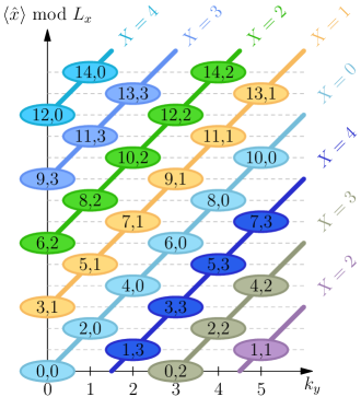
Figure 1: Relabeling of the Wannier states $|X,k_{y}\rangle\leftrightarrow|j,s\rangle$ for $(N_{x},N_{y})=(5,6)$ and $C=4$. We focus on the principal region with $X\in[{0~{}..~{}N_{x}})$ and $k_{y}\in[{0~{}..~{}N_{y}})$. Each solid ellipse represents a Wannier center. The horizontal axis gives the $k_{y}$ index while the vertical axis gives the position of the Wannier center in the $x$ direction (mod $L_{x}$). The ellipses are colored according to the $X$ index, and labeled by the $(j,s)$ indices. We have employed Eq. (58) to shift $j$ to $[0~{}..~{}M)$ and $s$ to $[0~{}..~{}C)$. Upon a color-independent flux insertion, each Wannier center flows along the solid lines of its color.

We emphasize that $j$ and $s$ are not independent. This can be seen by examining the solutions to the first equation in Eq. (49). For a given $j$, if $(X,k_{y})$ is a solution, then all the solutions can be parametrized as $(X+nC/\widetilde{C},k_{y}-nN_{y}/\widetilde{C})$, $n\in\mathbb{Z}$. Therefore $s=X$ mod $C$ can take $\widetilde{C}$ different values in $[0~{}..~{}C)$ with uniform spacing $d=C/\widetilde{C}$ [Eq. (50)], corresponding to $n=1,\ldots,\widetilde{C}$ in $X+nC/\widetilde{C}$. For a given $j$, we denote this set of $\widetilde{C}$ allowed values of $s$ by

$$S_{j}\subset[0~{}..~{}C).$$ (51)

A useful property is

$$S_{j}=S_{j+d},$$ (52)

which follows from the fact that $j\rightarrow j+d$ can be achieved by $k_{y}\rightarrow k_{y}+1$ without touching $X$. Plugging Eq. (49) into Eq. (16), we find that indeed we can relabel the hybrid Wannier states

$$|X,k_{y}\rangle\leftrightarrow|j,s\rangle,$$ (53)

modulo the identification

$$|j,s\rangle=|j,s+C\rangle.$$ (54)

An example is given in Fig. 1. It is not hard to see that this mapping is bijective, although we cannot easily write down an explicit formula for the solution $(X,k_{y})$ to Eq. (49) at a given $(j,s)$. We denote the $k_{y}$ solution formally as

$$k_{y}(j,s).$$ (55)

Then, the representation of the color-entangled magnetic translations $\widetilde{T}_{\alpha}$ in the $|j,s\rangle$ basis can be constructed indirectly from Eq. (18),

$$\widetilde{T}_{x}|j,s\rangle =|j+N_{y}/\widetilde{C},s+1\rangle,$$ (56)

$$\widetilde{T}_{y}|j,s\rangle =e^{-i2\pi k_{y}(j,s)/N_{y}}|j,s\rangle.$$

The wave functions for $|j,s\rangle$ can be obtained from Eq. (16),

$$\langle x,y,\sigma|j,s\rangle=\frac{1}{(\sqrt{\pi}L_{y}l_{B})^{1/2}}\sum_{m}^{\mathbb{Z}}\delta_{\sigma,s+mN_{x}}^{\text{mod }C}\\ \exp\Big{\{}\textstyle i2\pi\!\left(\frac{j}{d}+mN_{\phi}\right)\frac{y}{L_{y}}-\frac{1}{2}\!\left[\frac{x}{l_{B}}\!-\!\frac{2\pi l_{B}}{L_{y}}\left(\frac{j}{d}+mN_{\phi}\right)\right]^{2}\!\Big{\}}.$$ (57)

In parallel to Eq. (17), $|j,s\rangle$ is periodic in $s$ but quasi-periodic in $j$,

$$|j+M,s+N_{x}\rangle =|j,s\rangle,$$ (58)

$$|j,s+C\rangle =|j,s\rangle.$$

As we will see soon, this twist in $s$ when shifting $j$ is the main issue that sets the current problem apart from the usual multicomponent FQH. Estienne and Bernevig (2012)

We now want to expand the projected density operator in the relabeled hybrid Wannier basis. On the one hand, notice that due to the quasi-periodicity of $|X,k_{y}\rangle$ [Eq. (17)], the double sum of $(X,k_{y})$ over $[0~{}..~{}N_{x})\times[0~{}..~{}N_{y})$ in Eq. (44) can be shifted to any set of $N_{x}N_{y}$ points in the $\mathbb{Z}^{2}$ plane, as long as the corresponding hybrid states are independent from each other. On the other hand, notice that

$$\Big{\{}\,|j,s\rangle\,\Big{|}\,j\in[j_{0}~{}..~{}j_{0}+M),s\in S_{j}\Big{\}}$$ (59)

label a set of $N_{x}N_{y}$ hybrid Wannier states that are independent from each other for any given $j_{0}\in\mathbb{Z}$. Therefore, we can rewrite the double sum in Eq. (44) as a sum over the above set. Since increasing $k_{y}$ by $q_{y}$ while keeping $X$ constant sends $(j,s)$ to $(j+q_{y}d,s)$, we have

$$\rho_{\mathbf{q}}=e^{-\mathbf{q}^{2}l_{B}^{2}/4}\sum_{j}^{M}\!{}^{\prime}e^{-i2\pi q_{x}(j+\frac{q_{y}d}{2})/M}\sum_{s}^{S_{j}}|j,s\rangle\langle j+q_{y}d,s|,$$ (60)

where the primed sum is over $j\in[j_{0}~{}..~{}j_{0}+M)$ for an arbitrary $j_{0}\in\mathbb{Z}$, with $M=N_{x}N_{y}/\widetilde{C}$ [Eq. (50)]. The appearance of $\langle j+q_{y}d,s|$ requires special attention: when we shift $j+q_{y}d$ back to $[j_{0}~{}..~{}j_{0}+M)$ using Eq. (58), the $s$ index must be changed accordingly, by $N_{x}$ (mod $C$). This boundary effect dictates that $\rho_{\mathbf{q}}$ is not diagonal in $s$ unless $N_{x}$ is divisible by $C$, which discourages a seemingly plausible interpretation of $s$ as an effective spin index in general.

III.2 Interacting Hamiltonian

We consider only interactions between a pair of color-neutral densities $\rho_{\mathbf{q}}$. The relevance of such interactions to the Chern insulators was justified numerically in our previous paper Wu et al. (2013b). Such interactions can be specified in terms of the Haldane pseudopotentials. Higher-body pseudopotentialsSimon et al. (2007) can be implemented in the same spirit. We consider only the first two pseudopotentials $(V_{0},V_{1})$ being non-negative, with all $V_{m>1}=0$. The interaction strength at momentum transfer $\mathbf{q}$ then reads

$$V_{\mathbf{q}}=4\pi l_{B}^{2}[V_{0}+V_{1}\cdot(1-\mathbf{q}^{2}l_{B}^{2})],$$ (61)

and the Hamiltonian is given by

$$H=\frac{1}{2L_{x}L_{y}}\sum_{\mathbf{q}}V_{\mathbf{q}}\rho_{\mathbf{q}}\rho_{-\mathbf{q}}.$$ (62)

Here $\mathbf{q}$ is summed over the infinite reciprocal lattice.

As shown in our previous paper Wu et al. (2013b), the color-entangled generalizations of the bosonic/fermionic Halperin singlet states and the corresponding quasihole states are defined as the exact zero modes of the above Hamiltonian (using $V_{1}=0$ for the bosonic case). These states are distinct from the usual Halperin states due to the color-entangled boundary conditions inherent in $\rho_{\mathbf{q}}$. Through numerical diagonalization, we can obtain these zero modes, and then transcribe them to the lattice system of an arbitrary Chern insulator using the one-body mapping between the LLL Bloch states and the lattice Bloch states. We now attempt to achieve an analytic understanding of this Hamiltonian, by exploiting its assumed adiabatic connectivity Wu et al. (2013b) to the thin-torus limit.

We first plug Eq. (60) into Eq. (62) and write $H$ in the relabeled hybrid Wannier basis,

$$\!\!H\!=\frac{1}{2L_{x}L_{y}}\!\!\sum_{\mathbf{q}}e^{-\mathbf{q}^{2}l_{B}^{2}/2}V_{\mathbf{q}}\sum_{j_{1}}^{M}\!{}^{\prime}\sum_{j_{2}}^{M}\!{}^{\prime}e^{-i2\pi q_{x}(j_{1}-j_{2}+q_{y}d)/M}\\ \sum_{s_{1}}^{S_{j_{1}}}\!\sum_{s_{2}}^{S_{j_{2}}}\psi^{\dagger}_{j_{1},s_{1}}\psi^{\dagger}_{j_{2},s_{2}}\psi_{j_{2}-q_{y}d,s_{2}}\psi_{j_{1}+q_{y}d,s_{1}},$$ (63)

where $M$ and $d$ are defined in Eq. (50), and for $\mathbf{q}=(2\pi q_{x}/L_{x},2\pi q_{y}/L_{y})$, we have

$$\mathbf{q}^{2}l_{B}^{2}=\frac{2\pi}{N_{\phi}}\left(\frac{L_{y}}{L_{x}}q_{x}^{2}+\frac{L_{x}}{L_{y}}q_{y}^{2}\right).$$ (64)

We want to massage the above expansion of $H$ to a form amenable to justified truncation in the thin-torus limit. The main obstacle is obviously the oscillatory factor $e^{-i2\pi q_{x}(j_{1}-j_{2}+q_{y}d)/M}$ in the coefficient. This can be removed in exchange for a Gaussian factor by performing a Poisson resummation over $q_{x}$, which does not appear in the index of the creation/annihilation operators. After some straightforward but tedious algebra in Appendix C, we find

$$\!\!\!H=\sqrt{\frac{L_{x}}{N_{\phi}L_{y}}}\sum_{q_{y}}^{\mathbb{Z}}e^{-\beta(q_{y}d)^{2}}\sum_{j}^{M}\!{}^{\prime}\sum_{\Delta}\sum_{n}^{\mathbb{Z}}e^{-\beta(\Delta-q_{y}d+nM)^{2}}\\ \left\{V_{0}+2\beta V_{1}\left[(\Delta-q_{y}d+nM)^{2}-(q_{y}d)^{2}\right]\right\}\\ \sum_{s}^{S_{j}}\sum_{s^{\prime}}^{S_{j+\Delta}}\psi^{\dagger}_{j,s}\psi^{\dagger}_{j+\Delta,s^{\prime}}\psi_{j+\Delta-q_{y}d,s^{\prime}}\psi_{j+q_{y}d,s},$$ (65)

where $\Delta$ is summed over an interval of length $M$ centered around $q_{y}d$,

$$\Delta\in\big{[}\,q_{y}d-\lfloor M/2\rfloor~{}..~{}q_{y}d-\lfloor M/2\rfloor+M\,\big{)},$$ (66)

and we have defined the shorthand

$$\beta=\frac{1}{d^{2}}\frac{\pi}{N_{\phi}}\frac{L_{x}}{L_{y}}.$$ (67)

IV Thin-Torus Analysis

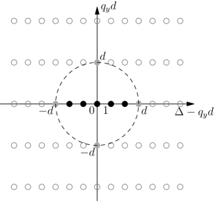
Figure 2: Terms in the expansion of the pseudopotential Hamiltonian. Here we illustrate the example of $d=3$. Each dot represents a term $(q_{y},\Delta)$ in Eq. (69). The weight of each term decays exponentially in its distance from the origin. The dashed circle marks the empirical threshold for truncation $(q_{y}d)^{2}+(\Delta-q_{y}d)^{2}=d^{2}$. The solid black dots inside are the density-density terms in Eq. (72), while the four solid gray dots contain the pair hopping and the density-density terms in Eqs. (75) and (85).

In Eq. (65), the Hamiltonian has been organized into groups of density-density or pair hopping terms. The strengths of the terms decay exponentially in the limit

$$\beta\gg 1.$$ (68)

This is exactly the thin-torus limit in Eq. (43). In the following, we perform a proper truncation of the Hamiltonian in this limit and analyze the degeneracy and quantum numbers of its zero modes.

The thin-torus analysis is a well-known, powerful technique to tackle the strongly-correlated physics in single-component FQH effect. Bergholtz and Karlhede (2005, 2006, 2008); Bernevig and Regnault (2012b) In the thin-torus limit, the pair hopping terms die off quickly, and the Hamiltonian becomes classical, dominated by density-density terms and thus solvable. (This is not true for certain non-unitary states Papic et al. .) One can obtain the correct degeneracy of the ground states and extract their total momenta simply by minimizing the classical electrostatic energy and completely ignoring the pair hoppings. By assumed adiabatic connectivity, Wu et al. (2013b) the results must also apply to the isotropic limit. The thin-torus analysis thus provides an intuitive picture for the ‘root partitions’ and the underlying generalized Pauli principle of Refs. Bernevig and Haldane, 2008a, b. Our multicomponent pseudopotential Hamiltonian with color-entangled boundaries (65) turns out to be considerably more complicated, due to the essential role played by the pair hopping terms. As we will see soon, the largest pair hopping terms have strengths comparable to the subleading density-density terms. Keeping only the leading density-density terms results in too many zero modes compared with the numerical studies Sterdyniak et al. (2013); Liu et al. (2012); Wu et al. (2013b). The correct ground-state degeneracy is recovered only after we put back the largest pair hoppings, which turn out to be of similar strength as some of the density-density terms. This indicates that the thin-torus limit of our multicomponent pseudopotential Hamiltonian cannot be described by classical electrostatics alone. The useful result of this Section is a set of rules [Sec. IV.4] that correctly predict the degeneracy and total lattice momenta of FCI ground states (including quasiholes). This is illustrated by explicit examples in Secs. IV.5 and IV.6.

IV.1 Truncation of Bosonic Hamiltonian

Numerical studies in Refs. Sterdyniak et al., 2013; Liu et al., 2012 found gapped FCI phases of bosons at filling $\nu=1/(C+1)$ with $(C+1)$-fold degenerate ground states, stabilized by on-site interactions projected to a topological flat band with Chern number $C$. In the following we specialize to the simplest case of bosons and try to understand the ground states of the pseudopotential Hamiltonian at filling $\nu=1/(C+1)$ and with quasiholes. Setting $V_{0}=\sqrt{N_{\phi}L_{y}/L_{x}}>0$ and $V_{1}=0$, the Hamiltonian in Eq. (65) becomes

$$H=\sum_{q_{y}}^{\mathbb{Z}}\sum_{j}^{M}\!{}^{\prime}\sum_{\Delta}\sum_{n}^{\mathbb{Z}}e^{-\beta(q_{y}d)^{2}-\beta(\Delta-q_{y}d+nM)^{2}}\\ \sum_{s}^{S_{j}}\sum_{s^{\prime}}^{S_{j+\Delta}}\psi^{\dagger}_{j,s}\psi^{\dagger}_{j+\Delta,s^{\prime}}\psi_{j+\Delta-q_{y}d,s^{\prime}}\psi_{j+q_{y}d,s}.$$ (69)

where the primed sum of $j$ is over

$$j\in[j_{0}~{}..~{}j_{0}+M)$$ (70)

for an arbitrary $j_{0}\in\mathbb{Z}$ [Eq. (59)], while $\Delta$ is summed over the interval of length $M$ given in Eq. (66).

In the $\beta\gg 1$ limit, we can safely truncate the sum over $n$ to a single term at $n=0$, if we assume that $M/d=N_{\phi}\gg 1$. Further, only the terms with $q_{y}\sim 0$ and $\Delta-q_{y}d\sim 0$ have a significant contribution, since the coefficients decay exponentially with respect to the (squared) Euclidean distance from $q_{y}d=\Delta-q_{y}d=0$,

$$R^{2}(q_{y},\Delta)\equiv(q_{y}d)^{2}+(\Delta-q_{y}d)^{2},$$ (71)

as illustrated in Fig. 2. The 4-boson $\psi^{\dagger}\psi^{\dagger}\psi\psi$ operator can be either density-density interaction or pair hopping. We find that the terms with $q_{y}=0$ are all density-density interactions, while the strongest pair hopping terms may appear at $|q_{y}|=1$, $\Delta=q_{y}d$, with Euclidean distance $R^{2}=d^{2}$.

In light of the previous studies Bergholtz and Karlhede (2005, 2006, 2008); Bernevig and Regnault (2012b), we first examine the effect of the terms with $R^{2}(q_{y},\Delta)<d^{2}$. They can be collected into

$$H_{<d^{2}}=\sum_{j}^{M}\sum_{\Delta}^{(-d~{}..~{}d)}e^{-\beta\Delta^{2}}n_{j}n_{j+\Delta},$$ (72)

where the number operator $n_{j}$ is defined by

$$n_{j}=\sum_{s}^{S_{j}}\psi^{\dagger}_{j,s}\psi_{j,s}.$$ (73)

Recall from Eq. (51) that $S_{j}$ is the set of all allowed values of $s$ for $\psi_{j,s}$ at a given $j$, and this set contains $\widetilde{C}$ different values. Also, recall from Eq. (50) that $d\,\widetilde{C}=C$. By solving the simple electrostatics, we find that the zero modes of $H_{<d^{2}}$ with highest density appear at filling $\nu=1/C$. This leads to much more than $(C+1)$ zero modes at filling $1/(C+1)$, inconsistent with the findings from numerical diagonalization of actual FCI Hamiltonians. Sterdyniak et al. (2013); Liu et al. (2012). This is a clear signal that we should include more terms in the truncated Hamiltonian.

In the following we analyze the effect of the next strongest terms in Eq. (69), with Euclidean distance $R^{2}(q_{y},\Delta)=d^{2}$. They are located at $({|\Delta-q_{y}d|},|q_{y}d|)=(0,d)$ and $(d,0)$, represented by the four solid gray dots in Fig. 2. In the next section we provide detailed analysis of the simplest case with $d=1$. The results for general $d$ will be presented afterwards.

IV.2 Effect of Pair Hopping Terms: $d=1$

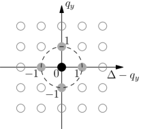
Figure 3: Terms in the expansion of the pseudopotential Hamiltonian at $d=1$. The presentation follows the same format as Fig. 2.

In this subsection we specialize to the simplest case $d=1$, illustrated in Fig. (3). In this case $N_{y}$ is divisible by $C$ [Eqs. (48) and (50)]. The pseudopotential Hamiltonian in Eq. (69) (after truncating the sum over $n$) becomes

$$H=\sum_{q_{y}}^{\mathbb{Z}}\sum_{j}^{M}\!{}^{\prime}\sum_{\Delta}e^{-\beta q_{y}^{2}-\beta(\Delta-q_{y})^{2}}\\ \sum_{s}^{S_{j}}\sum_{s^{\prime}}^{S_{j+\Delta}}\psi^{\dagger}_{j,s}\psi^{\dagger}_{j+\Delta,s^{\prime}}\psi_{j+\Delta-q_{y},s^{\prime}}\psi_{j+q_{y},s}.$$ (74)

We now extract the terms at $q_{y}^{2}+(\Delta-q_{y})^{2}=d^{2}=1$, namely, at $(q_{y},\Delta)=(1,1),(0,1),(-1,-1),(0,-1)$. To collect together the terms nicely, recall from Eq. (52) that $S_{j}=S_{j+1}$ at $d=1$, and note that we can take advantage of the freedom in Eq. (70) to shift the range of the primed sum over $j$. We then find

$$\sum_{j}^{M}e^{-\beta}\sum_{s}^{S_{j}}\sum_{s^{\prime}}^{S_{j}}\Big{[}(1,1)+(0,1)+(-1,-1)+(0,-1)\Big{]}.$$ (75)

The four terms in the above brackets are labeled by $(q_{y},\Delta)$, and explicitly they are given by

$$\psi^{\dagger}_{j,s}\psi^{\dagger}_{j+1,s^{\prime}}\psi_{j,s^{\prime}}\psi_{j+1,s}\!+\psi^{\dagger}_{j,s}\psi^{\dagger}_{j+1,s^{\prime}}\psi_{j+1,s^{\prime}}\psi_{j,s}$$ (76)

$$+ \psi^{\dagger}_{j+1,s}\psi^{\dagger}_{j,s^{\prime}}\psi_{j+1,s^{\prime}}\psi_{j,s}\!+\psi^{\dagger}_{j+1,s}\psi^{\dagger}_{j,s^{\prime}}\psi_{j,s^{\prime}}\psi_{j+1,s}.$$

Further, notice that we can combine the above four terms into a single product,

$$b^{\dagger}_{j,s,s^{\prime}}b_{j,s,s^{\prime}},$$ (77)

where the pair annihilation operator is given by

$$b_{j,s,s^{\prime}}=\psi_{j,s^{\prime}}\psi_{j+1,s}+\psi_{j+1,s^{\prime}}\psi_{j,s}.$$ (78)

This combination is the key to the enumeration of zero modes as we detail below. Together with the density-density terms in Eq. (72), the bosonic pseudopotential Hamiltonian takes the truncated form

$$H=\sum_{j}^{M}\Bigg{[}n_{j}n_{j}+e^{-\beta}\bigg{(}2n_{j}n_{j+1}+\sum_{s}^{S_{j}}\sum_{s^{\prime}}^{S_{j}}b^{\dagger}_{j,s,s^{\prime}}b_{j,s,s^{\prime}}\bigg{)}\Bigg{]}\\ +\sum_{j}^{M}\,\mathcal{O}\Big{(}e^{-2\beta}\Big{)}.$$ (79)

The residual terms are exponentially small for $\beta\gg 1$.

When $\widetilde{C}=1$, the $s$ index can take only a single value $s=0$, reducing $b_{j,s,s^{\prime}}$ to $2\psi_{j,0}\psi_{j+1,0}$. This includes the case of Chern number $C=1$. The truncated Hamiltonian becomes very simple:

$$H=\sum_{j}^{M}\left(n_{j}n_{j}+4e^{-\beta}n_{j}n_{j+1}\right)+\sum_{j}^{M}\,\mathcal{O}\Big{(}e^{-2\beta}\Big{)}.$$ (80)

Its zeros modes have no more than one boson in two consecutive orbitals. We thus recover the familiar result Bergholtz and Karlhede (2005); Bernevig and Haldane (2008a) for the bosonic Laughlin state at half filling.

We now come back to the case with generic $C$. We look for the constraints on the zero modes of the above truncated Hamiltonian in Eq. (79). Due to the two-body nature of the interaction, we only need to consider a pair of bosons at a time, with $j$ indices being $j_{1},j_{2}$. In Eq. (79), each term in the summation is positive-semidefinite by itself. This means that to find the zero modes of Eq. (79), we only need to identify the null space of each term individually, and then take their intersection. From the density-density terms, we find that in a zero mode we must have

$$|j_{1}-j_{2}|\geq 1.$$ (81)

This amounts to a minimal distance between adjacent bosons along the $j$ axis, with no discrimination of the $s$ indices. The pair hopping terms $\sum b^{\dagger}b$ in Eq. (79) kick in only when the equality sign is taken in Eq. (81), as is evident from Eq. (78). Specifically, $\sum b^{\dagger}b$ enforces in a zero mode the antisymmetrization of the $s$ indices between bosons with $|j_{1}-j_{2}|=1$,

$$\left(\psi^{\dagger}_{j_{1},s_{1}}\psi^{\dagger}_{j_{2},s_{2}}-\psi^{\dagger}_{j_{1},s_{2}}\psi^{\dagger}_{j_{2},s_{1}}\right)\,\big{|}\emptyset\big{\rangle}.$$ (82)

We emphasize that the $\psi^{\dagger}$’s are bosonic operators. It is easy to verify that the above antisymmetrized form is indeed annihilated by $\sum b^{\dagger}b$, whereas the symmetrized form acquires a positive energy $2e^{-\beta}$. To find the zero modes for a system of $N$ bosons, we need to perform the above procedure on each pair of bosons. This is explained in more details in Sec. IV.4, and illustrated by an example in Sec. IV.6.

One last subtlety comes from the quasi-periodicity of the $j$ index [Eq. (58)]. The orbitals at $j+M$ are identified with those at $j$, but there is a possible mismatch between the $s$ indices,

$$|j+M,s\rangle=|j,s-N_{x}\rangle.$$ (83)

For the density terms, this does not make much trouble since $n_{j}=n_{j+M}$ after the summation of the $s$ index over $S_{j}$ [Eq. (73)]; we just need to enforce the minimal distance condition [Eq. (81)] across the quasi-periodic boundary $j=0$ mod $M$. For the pair hopping terms, however, we have to be more careful about the $s$ index mismatch. We have to first shift their $j$ indices (by integer multiples of $M$) such that $|j_{1}-j_{2}|=1$ before we can apply the antisymmetrization in Eq. (82). More explicitly, if $|j_{1}-j_{2}+M|=1$ for example, then the correct antisymmetrization can be either of the following two equivalents,

$$\big{(}\psi^{\dagger}_{j_{1}+M,s_{1}}\psi^{\dagger}_{j_{2},s_{2}} -\psi^{\dagger}_{j_{1}+M,s_{2}}\psi^{\dagger}_{j_{2},s_{1}}\big{)}\,\big{|}\emptyset\big{\rangle}$$ (84)

$$=\big{(}\psi^{\dagger}_{j_{1},s_{1}-N_{x}}\psi^{\dagger}_{j_{2},s_{2}} -\psi^{\dagger}_{j_{1},s_{2}-N_{x}}\psi^{\dagger}_{j_{2},s_{1}}\big{)}\,\big{|}\emptyset\big{\rangle},$$

but not Eq. (82) anymore. This is the only reason why we were not able to consistently implement Wu et al. (2013b) the exclusion principle for conventional multicomponent FQH model states Estienne and Bernevig (2012); Ardonne and Regnault (2011) for the color-entangled system.

IV.3 Effect of Pair Hopping Terms: General $d$

The analysis for general $d$ is not much different from $d=1$. Here we just state the essential results. The pair hopping and density-density terms at $(q_{y}d)^{2}+({\Delta-q_{y}d})^{2}=d^{2}$ can be merged together,

$$\sum_{j}^{M}e^{-\beta d^{2}}\sum_{s}^{S_{j}}\sum_{s^{\prime}}^{S_{j}}b^{\dagger}_{j,s,s^{\prime}}b_{j,s,s^{\prime}},$$ (85)

where the two-body annihilation operator is given by

$$b_{j,s,s^{\prime}}=\psi_{j,s^{\prime}}\psi_{j+d,s}+\psi_{j+d,s^{\prime}}\psi_{j,s}.$$ (86)

Combined with the density-density terms in Eq. (72), the leading terms in the bosonic pseudopotential Hamiltonian in the limit of $\beta\gg 1$ are

$$H=\sum_{j}^{M}\Bigg{[}\sum_{\Delta}^{(-d~{}..~{}d)}e^{-\beta\Delta^{2}}n_{j}n_{j+\Delta}\\ +e^{-\beta d^{2}}\sum_{s}^{S_{j}}\sum_{s^{\prime}}^{S_{j}}b^{\dagger}_{j,s,s^{\prime}}b_{j,s,s^{\prime}}\Bigg{]}\\ +\sum_{j}^{M}\,\mathcal{O}\Big{(}e^{-\beta(d^{2}+1)}\Big{)}.$$ (87)

The zero modes of the truncated Hamiltonian satisfy the following pairwise constraints. First, for a pair of bosons with $j$ indices being $j_{1}$ and $j_{2}$, we must have

$$|j_{1}-j_{2}|\geq d.$$ (88)

Here the difference in $j$ is understood with the quasi-periodic identification $j\sim j+M$. When the equality in Eq. (88) holds, the two bosons are further subject to an antisymmetrization in the $s$ indices. For the simplest case $|j_{1}-j_{2}|=d$, we need Eq. (82), whereas for $|j_{1}-j_{2}+M|=d$, we need either of the two equivalents in Eq. (84). When $\widetilde{C}=1$, as $s$ can take only one value, this antisymmetrization consistently reduces to an electrostatic repulsion at distance $|j_{1}-j_{2}|=d$ (and also $|j_{1}-j_{2}+M|=d$).

IV.4 Counting Rule for Degeneracy and Momenta

Following the above constraints, we can enumerate all the zero modes of the truncated Hamiltonian for a given system size and a given number of particles, in the form

$$\mathcal{A}\big{[}\,\psi^{\dagger}_{j_{1},s_{1}}\psi^{\dagger}_{j_{2},s_{2}}\psi^{\dagger}_{j_{3},s_{3}}\psi^{\dagger}_{j_{4},s_{4}}\cdots\,\big{]}\,|\emptyset\rangle,$$ (89)

where $\mathcal{A}$ antisymmetrizes the $s$ indices as follows. As noted earlier, for any pair of particles $a$ and $b$ in a zero mode, we must have $|j_{a}-j_{b}|\geq d$, and when the equality holds, we need to carry out antisymmetrization over the $s$ indices $(s_{a},s_{b})$. Obviously, if we have $j_{1}-j_{2}=d$ and $j_{2}-j_{3}=d$, then we need to antisymmetrize over $(s_{1},s_{2},s_{3})$. More generally, if we have a cluster of $m$ consecutive particles satisfying $j_{a}-j_{a+1}=d$, we need a full antisymmetrization over all the $s$ indices of these $m$ particles.

The last remaining step is to group these zero modes according by the total Bloch momentum and count the degeneracy per momentum sector. The resulting degeneracy is linked by the Bloch mapping Wu et al. (2013b) to the degeneracy of FCI ground states per lattice momentum sector. This largely follows the same procedure as detailed in Ref. Bernevig and Regnault, 2012a. We represent by lowercase $k_{\alpha}$ the Bloch momenta of individual particles in the $\alpha=x,y$ direction, and by uppercase

$$K_{\alpha}=\sum k_{\alpha}\text{ mod }N_{\alpha}$$ (90)

the total Bloch momentum of the many-body system (the summation is over particles). We denote by $\widetilde{T}^{\mathrm{cm}}_{\alpha}$ the center-of-mass color-entangled magnetic translations, i.e. applying $\widetilde{T}_{\alpha}$ simultaneously on all the particles. Then, the total Bloch momentum $K_{\alpha}$ can be read off from the eigenvalue of $\widetilde{T}^{\mathrm{cm}}_{\alpha}$,

$$\widetilde{T}^{\mathrm{cm}}_{\alpha}=e^{-i2\pi K_{\alpha}/N_{\alpha}}.$$ (91)

The action of $\widetilde{T}^{\mathrm{cm}}_{\alpha}$ on the zero modes in Eq. (89) is spelled out in Eq. (56).

There are four points to make here. First, the zero modes in the form of Eq. (89) are automatically eigenstates of $\widetilde{T}^{\mathrm{cm}}_{y}$. Evidently each term in the antisymmetrization $\mathcal{A}$ individually is an eigenstate of $\widetilde{T}^{\mathrm{cm}}_{y}$. Moreover, the eigenvalues have to be the same for all those terms. This follows from the linearity of Eq. (49): to find the total $\sum k_{y}$ of all particles, we only need to know the total $\sum j$ and $\sum s$; the actual association of between $j$ and $s$ does not matter. Second, under the action of $\widetilde{T}^{\mathrm{cm}}_{x}$, the zero modes in Eq. (89) form closed orbits. This follows from the fact that $\widetilde{T}^{\mathrm{cm}}_{x}$ commutes with the (truncated) pseudopotential Hamiltonian, and thus preserves its null space. More directly, one can easily verify that the constraints on the zero modes described in Secs. IV.2 and IV.3 are invariant under the action of $\widetilde{T}^{\mathrm{cm}}_{x}$ (namely $X\rightarrow X+1$, or $|\{j,s\}\rangle\rightarrow|\{j+N_{y}/\widetilde{C},s+1\}\rangle$), and that the action of $\widetilde{T}^{\mathrm{cm}}_{x}$ always brings one zero mode in the form of Eq. (89) to another zero mode in the same form. Third, each action of $\widetilde{T}^{\mathrm{cm}}_{x}$ along the orbit is associated with a sign, since a term in the antisymmetrization $\mathcal{A}$ in Eq. (89) may be brought to a term with the opposite sign. Fourth, all the zero modes in an orbit under $\widetilde{T}^{\mathrm{cm}}_{x}$ share the same eigenvalue under $\widetilde{T}^{\mathrm{cm}}_{y}$. This is a direct consequence of $[\widetilde{T}^{\mathrm{cm}}_{x},\widetilde{T}^{\mathrm{cm}}_{y}]=0$.

For each zero mode in the form of Eq. (89), we can directly compute the total $K_{y}$ momentum by just looking at a single term in the antisymmetrization $\mathcal{A}$. We can group together the zero modes by the value of $K_{y}=\sum k_{y}$ mod $N_{y}$. Then, within each group, we successively apply $\widetilde{T}^{\mathrm{cm}}_{x}$ on each zero mode and further break them into disjoint orbits. Consider an orbit consisting of $n$ zero modes $|0\rangle,|1\rangle,\ldots,|n-1\rangle$ of the form in Eq. (89). They are linked together by

$$\widetilde{T}^{\mathrm{cm}}_{x}|r\rangle=g_{r}\,|r+1\text{ mod }n\rangle,\quad r\in[0~{}..~{}n),$$ (92)

with $g_{r}=\pm 1$ determined from the action of $\widetilde{T}_{x}^{\mathrm{cm}}$ on the antisymmetrization in Eq. (89). The $n$ eigenstates of $\widetilde{T}^{\mathrm{cm}}_{x}$ are linear recombinations of these $n$ states in the form of Fourier sums. Without actually writing down the linear recombinations, we can directly obtain the eigenvalues. By successively applying the above equation, we find

$$[\widetilde{T}^{\mathrm{cm}}_{x}]^{n}\,|r\rangle=g\,|r\rangle,$$ (93)

with $g=\prod_{r^{\prime}}^{n}g_{r^{\prime}}$. This fixes the $n$ eigenvalues of $\widetilde{T}^{\mathrm{cm}}_{x}$ to be the $n$ distinct $n$-th roots of $g$. If $g=1$, the total $K_{x}$ momenta of the zero modes are

$$K_{x}=k\frac{N_{x}}{n}\text{ mod }N_{x},\quad k\in[0~{}..~{}n),$$ (94)

whereas if $g=-1$, they are

$$K_{x}=k\frac{N_{x}}{n}+\frac{N_{x}}{2}\text{ mod }N_{x},\quad k\in[0~{}..~{}n).$$ (95)

The numbers on the right hand side of the above equation are guaranteed to be integers: Since $[\widetilde{T}^{\mathrm{cm}}_{x}]^{N_{x}}$ is the identity operator per the color-entangled boundary condition [Eq. (13)], we must have $N_{x}/n\in\mathbb{Z}$, and also $g^{N_{x}/n}=1$.

Our end goal is an analytic algorithm to obtain the degeneracy of the zero modes in each Bloch momentum sector. This request is more modest than to find the actual expression of the zero modes in each sector, and the above procedure can be further simplified. For example, we do not need to actually write down the zero modes as in Eq. (89). We only need to keep track of the structure of clusters of consecutive particles with $j_{a}-j_{a+1}=d$, as noted below Eq. (89), and the set of $s$ indices in each cluster. An open-source reference implementation can be found at http://fractionalized.github.io. We have tested our algorithm extensively against the total Bloch momenta of the actual ground states obtained from numerical diagonalization for various system sizes, and found perfect agreement across all cases.

IV.5 A Simple Example

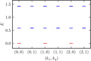
Figure 4: Energy spectrum of the pseudopotential Hamiltonian of 2 bosons on a $N_{x}\times N_{y}=3\times 2$ lattice with Chern number $C=2$. The three degenerate ground states at zero energy are marked in red.

To see the above counting rule in action, we consider a simple example, 2 bosons on a $N_{x}\times N_{y}=3\times 2$ lattice with Chern number $C=2$. From numerical diagonalization of the pseudopotential Hamiltonian (see Fig. 4), we find 3-fold degenerate ground states with total Bloch momenta

$$(K_{x},K_{y})=(0,0),(1,0),(2,0)\text{ mod }(3,2).$$ (96)

We note that the spinless counting rule Bernevig and Regnault (2012a) gives the wrong result $K_{y}=1$ mod $2$ when naively applied to this system. We now show how our new procedure produces the correct momenta.

From $(N_{x},N_{y})=(3,2)$ and $C=2$, we compute $\widetilde{C}=\mathrm{GCD}(C,N_{y})=2$, $d=C/\widetilde{C}=1$, $M=N_{x}N_{y}/\widetilde{C}=3$. Equation (49) reduces to

$$j =X+k_{y},$$ (97)

$$s =X\text{ mod }2.$$

We denote $s=0$ by $\downarrow$ and $s=1$ by $\uparrow$. To facilitate two-way lookup of the mapping $(X,k_{y})\leftrightarrow(j,s)$, we can make a table

$$X$$

0 0 0

0 1 1

1 0 1

1 1 2

2 0 2

2 1 0

(98)

The last line in the above table deserves special attention. From Eq. (97), for $(X,k_{y})=(2,1)$ we obtain $(j,s)={(3,\downarrow)}$. However, due to the quasi-periodicity condition in $j$, [Eq. (58)], this is equivalent to $(j,s)={(0,\uparrow)}$.

We enumerate all the two-boson zero modes of the truncated pseudopotential Hamiltonian [Eq. (87)] in the form of Eq. (89). Applying the constraint $|j_{1}-j_{2}|\geq 1$ across the quasi-periodic boundary of $j$, we find only three possibilities

$$(j_{1},j_{2})=(0,1),(1,2),(0,2).$$ (99)

All of them satisfy either $|j_{1}-j_{2}|=d$ (first two) or $|j_{1}-j_{2}+M|=d$ (last one), and are thus subject to full antisymmetrization of the $s$ indices $(s_{1},s_{2})$. Since there are only two allowed values of $s$, we can already see that there are only 3 zero modes in the form of Eq. (89). We now go through them one by one. First, consider $(j_{1},j_{2})=(0,1)$. Using Eq. (82), we find that the only possible $(s_{1},s_{2})$ antisymmetrization is

$$|0,1\rangle\!\rangle\equiv\left(\psi^{\dagger}_{0,\downarrow}\psi^{\dagger}_{1,\uparrow}-\psi^{\dagger}_{0,\uparrow}\psi^{\dagger}_{1,\downarrow}\right)\,\big{|}\emptyset\big{\rangle}.$$ (100)

Here the double bracket $|\cdot,\cdot\rangle\!\rangle$ distinguishes the many-body zero mode from the one-body basis state $|j,s\rangle$, and the subscript of the creation operator $\psi^{\dagger}$ denotes $(j,s)$. Similarly, for $(j_{1},j_{2})=(1,2)$, we find

$$|1,2\rangle\!\rangle\equiv\left(\psi^{\dagger}_{1,\downarrow}\psi^{\dagger}_{2,\uparrow}-\psi^{\dagger}_{1,\uparrow}\psi^{\dagger}_{2,\downarrow}\right)\,\big{|}\emptyset\big{\rangle}.$$ (101)

The case of $(j_{1},j_{2})=(0,2)$ satisfies $|j_{1}-j_{2}+M|=d$ rather than $|j_{1}-j_{2}|=d$. So we use Eq. (84) rather than Eq. (82), and find

$$|0,2\rangle\!\rangle \equiv\left(\psi^{\dagger}_{3,\downarrow}\psi^{\dagger}_{2,\uparrow}-\psi^{\dagger}_{3,\uparrow}\psi^{\dagger}_{2,\downarrow}\right)\,\big{|}\emptyset\big{\rangle}$$ (102)

$$=\left(\psi^{\dagger}_{0,\uparrow}\psi^{\dagger}_{2,\uparrow}-\psi^{\dagger}_{0,\downarrow}\psi^{\dagger}_{2,\downarrow}\right)\,\big{|}\emptyset\big{\rangle}.$$

Notice that after we bring the $j$ indices back to $[0~{}..~{}M)$ using Eq. (83), the $s$ indices on the second line are not in an explicit antisymmetrized form. This manifests the core difference of our problem from the usual FQH: When the lattice size is incommensurate with the Chern number, we cannot consistently distinguish the $C$ families of Wannier states, since the flow of Wannier centers are entangled on the quasi-perioidic boundary.

Using the lookup table in Eq. (98), we find that the total $K_{y}$ momenta of the three zero modes are all equal to $0$ mod $2$, consistent with Eq. (96). To compute the $K_{x}$ momentum, we need to find out the action of the center-of-mass translation $\widetilde{T}_{x}^{\mathrm{cm}}$ on these states. For our example, Equation (56) reduces to

$$\widetilde{T}_{x}|j,s\rangle=|j+1,s+1\rangle.$$ (103)

We thus find the representation of $\widetilde{T}_{x}^{\mathrm{cm}}$ on the zero modes:

$$\widetilde{T}_{x}^{\mathrm{cm}}|0,1\rangle\!\rangle =\left(\psi^{\dagger}_{1,\uparrow}\psi^{\dagger}_{2,\downarrow}-\psi^{\dagger}_{1,\downarrow}\psi^{\dagger}_{2,\uparrow}\right)\big{|}\emptyset\big{\rangle}=-|1,2\rangle\!\rangle,$$ (104)

$$\widetilde{T}_{x}^{\mathrm{cm}}|1,2\rangle\!\rangle =\left(\psi^{\dagger}_{2,\uparrow}\psi^{\dagger}_{3,\downarrow}-\psi^{\dagger}_{2,\downarrow}\psi^{\dagger}_{3,\uparrow}\right)\big{|}\emptyset\big{\rangle}=|0,2\rangle\!\rangle,$$

$$\widetilde{T}_{x}^{\mathrm{cm}}|0,2\rangle\!\rangle =\left(\psi^{\dagger}_{1,\downarrow}\psi^{\dagger}_{3,\downarrow}-\psi^{\dagger}_{1,\uparrow}\psi^{\dagger}_{3,\uparrow}\right)\big{|}\emptyset\big{\rangle}$$

$$=\left(\psi^{\dagger}_{1,\downarrow}\psi^{\dagger}_{0,\uparrow}-\psi^{\dagger}_{1,\uparrow}\psi^{\dagger}_{0,\downarrow}\right)\big{|}\emptyset\big{\rangle}=-|0,1\rangle\!\rangle.$$

Notice that we can evaluate $\widetilde{T}_{x}^{\mathrm{cm}}|0,2\rangle\!\rangle$ using either line in Eq. (102); the results are guaranteed to be the same by the consistency between Eqs. (56) and (58).

The three zero modes thus form a single orbit under the successive action of $\widetilde{T}_{x}^{\mathrm{cm}}$. They can be recombined to form eigenstates of $\widetilde{T}_{x}^{\mathrm{cm}}$. To find the total $K_{x}$ momenta of the recombined states, we can either follow the procedure detailed in the last subsection, or we can brute-force diagonalize $\widetilde{T}_{x}^{\mathrm{cm}}$. The representation matrix of $\widetilde{T}_{x}^{\mathrm{cm}}$ over the three zero modes reads

$$\left(\begin{array}[]{ccc}0&-1&0\\ 0&0&1\\ -1&0&0\end{array}\right).$$ (105)

From its eigenvalues $\{1,e^{i2\pi/3},e^{-i2\pi/3}\}$, we find the total $K_{x}$ momenta of the three recombined zero modes to be $0,1,2$ mod $3$. In summary, we reproduce the correct total Bloch momenta in Eq. (96).

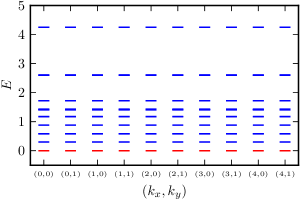
Figure 5: Energy spectrum of the pseudopotential Hamiltonian of 3 bosons on a $N_{x}\times N_{y}=5\times 2$ lattice with Chern number $C=2$. The 10 degenerate ground states at zero energy are marked in red.

IV.6 An Example with Quasiholes

Next, we consider a slightly more complicated example with quasiholes. For a system of 3 bosons with $C=2$, the densest zero modes of our pseudopotential Hamiltonian occur at filling $\nu=1/(C+1)=1/3$, i.e. 3 bosons in $9/2$ fluxes. The fractional flux is possible thanks to the color-entangled boundary conditions in Eq. (13). We now add $\frac{1}{2}$ flux to each color component and consider $N_{x}\times N_{y}=5\times 2$ and $N_{\phi}=9/2+1/2=N_{x}N_{y}/C=5$. This leads to a set of 10-fold degenerate quasihole states at zero energy, with one mode in each momentum sector $(K_{x},K_{y})\in[0~{}..~{}N_{x})\times[0~{}..~{}N_{y})$. This can be seen in the numerical diagonalization results in Fig. 5.

We now show how to obtain this counting using our algorithm. The basic procedure is the same as the previous example. We first compute $\widetilde{C}=\mathrm{GCD}(C,N_{y})=2$, $d=C/\widetilde{C}=1$, and $M=N_{x}N_{y}/\widetilde{C}=5$. Equation (49) again reduces to Eq. (97), and we have two allowed values of $s$ ($0$ and $1$), denoted by $\downarrow$ and $\uparrow$. Then we can build the $(X,k_{y})\leftrightarrow(j,s)$ lookup table,

$$X$$

0 0 0

0 1 1

1 0 1

1 1 2

2 0 2

2 1 3

3 0 3

3 1 4

4 0 4

4 1 0

(106)

Again, the last line in the table has a flipped $s$ index due to the quasi-periodic boundary condition in $j$ [Eq. (58)].

Compared with the previous example, the enumeration of the zero modes in the form of Eq. (89) has an extra complication. Let us first apply the $|j_{a}-j_{b}|\geq 1$ rule between each pair of bosons. We find two groups of allowed $(j_{1},j_{2},j_{3})$ configurations,

$$(\underline{0,1,2}),(\underline{1,2,3}),(\underline{2,3,4}),(\underline{3,4,0}),(\underline{4,0,1}),$$ (107)

and

$$(\underline{0,1},3),(\underline{1,2},4),(\underline{2,3},0),(\underline{3,4},1),(\underline{4,0},2).$$ (108)

Here we have underlined each cluster of bosons linked together by $|j_{a}-j_{b}|=d=1$ or $|j_{a}-j_{b}+M|=d=1$. Then, we need to antisymmetrize the $s$ indices of the bosons in the same cluster. This kills the five configurations in the first group [Eq. (107)]: the three bosons in the same cluster must take different values of $s$ under antisymmetrization, but there are only two possible values of $s$ ($\uparrow$ and $\downarrow$). We are left with the five $j$ configurations in Eq. (108). In each configuration, the two clustered bosons have antisymmetrized $s$ indices $\uparrow\downarrow-\downarrow\uparrow$, while the third boson can take either $\uparrow$ or $\downarrow$. For example, for $(j_{1},j_{2},j_{3})=(0,1,3)$, we have a pair of zero modes

$$\left(\psi^{\dagger}_{0,\downarrow}\psi^{\dagger}_{1,\uparrow}-\psi^{\dagger}_{0,\uparrow}\psi^{\dagger}_{1,\downarrow}\right)\psi^{\dagger}_{3,\uparrow}\,\big{|}\emptyset\big{\rangle},$$ (109)

$$\left(\psi^{\dagger}_{0,\downarrow}\psi^{\dagger}_{1,\uparrow}-\psi^{\dagger}_{0,\uparrow}\psi^{\dagger}_{1,\downarrow}\right)\psi^{\dagger}_{3,\downarrow}\,\big{|}\emptyset\big{\rangle}.$$

We can similarly write down the other 8 zero modes. This gives the correct 10-fold degeneracy. Using the lookup table in Eq. (106), we can compute the $K_{y}$ lattice momentum for each zero mode and construct the representation matrix of the color-entangled center-of-mass translation operator $\widetilde{T}_{x}^{\mathrm{cm}}$ in exactly the same manner as in the previous example. This reproduces the correct degeneracy in each momentum sector. We leave details of this last step for the interested readers.

V Conclusion

In this paper we have studied the pseudopotential model Hamiltonian for FCI with an arbitrary Chern number. We establish a one-body mapping between a Chern band with Chern number $C$, and a $C$-component LLL with specially engineered boundary conditions. The new boundary conditions lead to an alternative set of pseudopotential Hamiltonians, and the corresponding zero modes define new model wave functions. By taking the thin-torus limit and keeping only the leading density-density and pair hopping terms, we are able to analytically solve the pseudopotential Hamiltonian and obtain its zero modes. By analyzing the representation of the center-of-mass translation operators, we derive an algorithm to directly compute the total Bloch momenta of the degenerate zero modes. As we showed in our last paper Wu et al. (2013b), our pseudopotential Hamiltonian is adiabatically connected to the lattice FCI Hamiltonian, and the its zero modes serve as good trial wave functions for the FCI ground states. In particular, there is a 1-to-1 correspondence between the trial wave function and the FCI ground state in each momentum sector. Therefore, our counting algorithm can be used to obtain the total lattice momenta of the FCI ground states (including quasiholes) without diagonalizing the FCI Hamiltonian, for Abelian FCI states at filling $\nu=1/(C+1)$.

Appendix A Hybrid Wannier States under Color-Entangled Magnetic Translations

In this Appendix we prove Eq. (18), the representation of $\widetilde{T}_{x}$ and $\widetilde{T}_{y}$ in the hybrid Wannier basis $|X,k_{y}\rangle$.

In Landau gauge $\mathbf{A}=Bx\hat{y}$, the magnetic translation operators $T_{x}$ and $T_{y}$ defined in Eq. (8) have the real-space representation

$$T_{x} =e^{i2\pi\frac{N_{\phi}}{N_{x}}\frac{y}{L_{y}}}e^{-\frac{L_{x}}{N_{x}}\partial_{x}},$$ (110)

$$T_{y} =e^{-\frac{L_{y}}{N_{y}}\partial_{y}}.$$

Acting on a trial state $|\psi\rangle$, they transform the real-space wave function $\langle x,y|\psi\rangle$ by

$$\langle x,y|T_{x}|\psi\rangle =e^{i2\pi\frac{N_{\phi}}{N_{x}}\frac{y}{L_{y}}}\langle x-L_{x}/N_{x},y|\psi\rangle,$$ (111)

$$\langle x,y|T_{y}|\psi\rangle =\langle x,y-L_{y}/N_{y}|\psi\rangle.$$

Plugging these into the Landau-gauge definition of $|X,k_{y}\rangle$ in Eq. (16) and using Eq. (2), we find

$$\langle x,y,\sigma|T_{x}|X,k_{y}\rangle =\langle x,y,\sigma+1|X+1,k_{y}\rangle,$$ (112)

$$\langle x,y,\sigma|T_{y}|X,k_{y}\rangle =e^{-i2\pi(k_{y}/N_{y}+\sigma/C)}\langle x,y,\sigma|X,k_{y}\rangle.$$

Since the clock-and-shift operators $Q,P$ defined in Eq. (10) are unitary, we have

$$\langle\sigma|P =\langle{\sigma-1}|, \langle\sigma|Q =e^{i2\pi\sigma/C}\langle\sigma|.$$ (113)

Putting Eqs. (112) and (113) together, we find the action of $\widetilde{T}_{x}=T_{x}P$ and $\widetilde{T}_{y}=T_{y}Q$ to be particularly simple,

$$\langle x,y,\sigma|\widetilde{T}_{x}|X,k_{y}\rangle =\langle x,y,\sigma|X+1,k_{y}\rangle,$$ (114)

$$\langle x,y,\sigma|\widetilde{T}_{y}|X,k_{y}\rangle =e^{-i2\pi k_{y}/N_{y}}\langle x,y,\sigma|X,k_{y}\rangle.$$

This proves Eq. (18).

Appendix B Projected Density in Bloch Basis

In this Appendix we prove Eq. (27), the expansion of the projected density operator in the Bloch basis, proof which, due to lack of space, was not included in Ref. Wu et al., 2013b.

We first derive a simpler form for the Bloch wave function $\phi_{\mathbf{k}}(\mathbf{r},\sigma)=\langle\mathbf{r},\sigma|\mathbf{k}\rangle$. When we plug Eq. (16) into Eq. (19), we have a double sum over $X,m$. However, notice that $(X,m)$ in the double sum can always be combined into $X+mN_{x}$, thanks to $XN_{y}/C+mN_{\phi}=(X+mN_{x})N_{y}/C$ and $e^{i2\pi Xk_{x}/N_{x}}=e^{i2\pi(X+mN_{x})k_{x}/N_{x}}$ (recall that $N_{\phi}=N_{x}N_{y}/C$). This enables us to merge the double sum into a single sum of $X+mN_{x}$ over $\mathbb{Z}$. The Kronecker-$\delta$ enforcing $\sigma=X+mN_{x}$ mod $C$ suggests we split $X+mN_{x}\rightarrow nC+\sigma$ with $n$ summed over $\mathbb{Z}$. This leads to the final form of the Bloch wave function,

$$\langle x,y,\sigma|\mathbf{k}\rangle=\frac{1}{(\sqrt{\pi}N_{x}L_{y}l_{B})^{1/2}}\sum_{n}^{\mathbb{Z}}e^{i2\pi(nC+\sigma)k_{x}/N_{x}}\\ \exp\left\{i2\pi\left(k_{y}+nN_{y}+\frac{\sigma}{C}N_{y}\right)\frac{y}{L_{y}}-\frac{1}{2}\left[\frac{x}{l_{B}}-\frac{2\pi l_{B}}{L_{y}}\left(k_{y}+nN_{y}+\frac{\sigma}{C}N_{y}\right)\right]^{2}\right\}.$$ (115)

This wave function indeed depends only on $\sigma$ mod $C$ (by a re-shift in the dummy variable $n$), and it has the quasi-periodicity in $k_{y}$ as in Eq. (20). We now plug this into $\rho_{\mathbf{q},\sigma}$ defined in Eq. (25).

$$\rho_{\mathbf{q},\sigma}=\frac{1}{\sqrt{\pi}N_{x}L_{y}l_{B}}\sum_{\mathbf{k}_{1}}^{\mathrm{BZ}}\sum_{\mathbf{k}_{2}}^{\mathrm{BZ}}|\mathbf{k}_{1}\rangle\langle\mathbf{k}_{2}|\sum_{n_{1}}^{\mathbb{Z}}\sum_{n_{2}}^{\mathbb{Z}}e^{-i2\pi(n_{1}C+\sigma)k_{1x}/N_{x}}e^{i2\pi(n_{2}C+\sigma)k_{2x}/N_{x}}\\ \left[\int_{0}^{L_{x}}\mathrm{d}x\,e^{-i2\pi q_{x}x/L_{x}}\exp\left\{-\frac{1}{2}\left[\frac{x}{l_{B}}-\frac{2\pi l_{B}}{L_{y}}\left(k_{1y}+\frac{\sigma}{C}N_{y}+n_{1}N_{y}\right)\right]^{2}-\frac{1}{2}\left[\frac{x}{l_{B}}-\frac{2\pi l_{B}}{L_{y}}\left(k_{2y}+\frac{\sigma}{C}N_{y}+n_{2}N_{y}\right)\right]^{2}\right\}\right]\\ \left[\int_{0}^{L_{y}}\mathrm{d}y\,e^{-i2\pi q_{y}y/L_{y}-i2\pi(k_{1y}+n_{1}N_{y}-k_{2y}-n_{2}N_{y})y/L_{y}}\right].$$ (116)

We first finish the $\int\mathrm{d}y$ integral on the last line,

$$\int\mathrm{d}y\,e^{-i2\pi\cdots}=L_{y}\,\delta_{k_{2y}+n_{2}N_{y},\;k_{1y}+n_{1}N_{y}+q_{y}}.$$ (117)

Notice that the summations of $\mathbf{k}_{1}$ and $\mathbf{k}_{2}$ over BZ in the above equation are independent. To accommodate the Kronecker-$\delta$ in the above equation, we set the summation of $k_{1y}$ over $[0~{}..~{}N_{y})$, and the summation of $k_{2y}$ over $[q_{y}~{}..~{}N_{y}+q_{y})$. Then, the Kronecker-$\delta$ above can be decomposed into two separate Kronecker-$\delta$’s, enforcing

$$\begin{aligned} k_{2y}&=k_{1y}+q_{y},\\ n_{1}&=n_{2}.\end{aligned}$$ (118)

And we have

$$\rho_{\mathbf{q},\sigma}=\frac{1}{\sqrt{\pi}N_{x}l_{B}}\sum_{k_{1x}}^{N_{x}}\sum_{k_{2x}}^{N_{x}}\sum_{k_{y}}^{N_{y}}|k_{1x},k_{y}\rangle\langle k_{2x},{k_{y}+q_{y}}|\sum_{n}^{\mathbb{Z}}e^{i2\pi(nC+\sigma)(k_{2x}-k_{1x})/N_{x}}\\ \left[\int_{0}^{L_{x}}\mathrm{d}x\,e^{-i2\pi q_{x}x/L_{x}}\exp\left\{-\frac{1}{2}\left[\frac{x}{l_{B}}-\frac{2\pi l_{B}}{L_{y}}\left(k_{y}+\frac{\sigma}{C}N_{y}+nN_{y}\right)\right]^{2}-\frac{1}{2}\left[\frac{x}{l_{B}}-\frac{2\pi l_{B}}{L_{y}}\left(k_{y}+q_{y}+\frac{\sigma}{C}N_{y}+nN_{y}\right)\right]^{2}\right\}\right].$$ (119)

It is easy to check that $\rho_{\mathbf{q},\sigma}$ is indeed invariant under a shift of the dummy variable $k_{y}\rightarrow k_{y}+N_{y}$. We now tackle the $\int\mathrm{d}x$ integral in the bracket. We can collect terms and complete the square in the exponential. After some trivial but tedious algebra, the integrand becomes

$$e^{-\mathbf{q}^{2}l_{B}^{2}/4}\,e^{-i2\pi q_{x}(k_{y}+q_{y}/2+\sigma N_{y}/C+nN_{y})/N_{\phi}}\exp\left\{-\left[\frac{x}{l_{B}}-\frac{2\pi l_{B}}{L_{y}}\left(k_{y}+\frac{\sigma}{C}N_{y}+nN_{y}+\frac{1}{2}\left(q_{y}-i\frac{L_{y}}{L_{x}}q_{x}\right)\right)\right]^{2}\right\}.$$ (120)

Here we have used $2\pi l_{B}^{2}N_{\phi}=L_{x}L_{y}$ [Eq. (2)], and

$$\mathbf{q}^{2}l_{B}^{2}=\frac{2\pi}{N_{\phi}}\left(\frac{L_{y}}{L_{x}}q_{x}^{2}+\frac{L_{x}}{L_{y}}q_{y}^{2}\right).$$ (121)

The projected density can thus be written as

$$\rho_{\mathbf{q},\sigma}=\frac{1}{\sqrt{\pi}N_{x}l_{B}}e^{-\mathbf{q}^{2}l_{B}^{2}/4}\sum_{k_{1x}}^{N_{x}}\sum_{k_{2x}}^{N_{x}}\sum_{k_{y}}^{N_{y}}|k_{1x},k_{y}\rangle\langle k_{2x},{k_{y}+q_{y}}|\,e^{-i2\pi q_{x}(k_{y}+q_{y}/2)/N_{\phi}}\\ \sum_{n}^{\mathbb{Z}}e^{i2\pi(nC+\sigma)(k_{2x}-k_{1x}-q_{x})/N_{x}}\ \int_{0}^{L_{x}}\mathrm{d}x\exp\left\{-\left[\frac{x}{l_{B}}-\frac{2\pi l_{B}}{L_{y}}\left(k_{y}+\frac{\sigma}{C}N_{y}+nN_{y}+\frac{1}{2}\left(q_{y}-i\frac{L_{y}}{L_{x}}q_{x}\right)\right)\right]^{2}\right\}.$$ (122)

Notice that

$$\frac{x}{l_{B}}-\frac{2\pi l_{B}}{L_{y}}nN_{y}=\frac{x-nN_{y}L_{x}/N_{\phi}}{l_{B}};$$ (123)

we can shift the integration interval to

$$\int_{n\frac{N_{y}}{N_{\phi}}L_{x}}^{L_{x}+n\frac{N_{y}}{N_{\phi}}L_{x}}\mathrm{d}x.$$ (124)

This moves the dependence on $n$ from the integrand to the integration limits (and also the exponential prefactor $e^{i2\pi(nC+\sigma)(k_{2x}-k_{1x}-q_{x})/N_{x}}$).

We want to sew together the integrals for all $n$ so that we can finish the Gaussian integral, but the integration intervals for different $n$ are overlapping and cannot be joined head to tail in general, unless $N_{x}$ is divisible by $C$. However, recall that (to have symmetries $P,Q$) we restrict the interacting Hamiltonian to be color-neutral, so we are interested only in $\rho_{\mathbf{q}}=\sum_{\sigma}^{C}\rho_{\mathbf{q},\sigma}$. The color sum saves us. Notice that the dependence on $(\sigma,n)$ is all through the combination $nC+\sigma$. We can merge the two sums over $\sigma$ and $n$ into a single sum over integers, $nC+\sigma\rightarrow m$:

$$\rho_{\mathbf{q}}=\frac{1}{\sqrt{\pi}N_{x}l_{B}}e^{-\mathbf{q}^{2}l_{B}^{2}/4}\sum_{k_{1x}}^{N_{x}}\sum_{k_{2x}}^{N_{x}}\sum_{k_{y}}^{N_{y}}|k_{1x},k_{y}\rangle\langle k_{2x},{k_{y}+q_{y}}|\,e^{-i2\pi q_{x}(k_{y}+q_{y}/2)/N_{\phi}}\\ \sum_{n}^{\mathbb{Z}}e^{i2\pi n(k_{2x}-k_{1x}-q_{x})/N_{x}}\ \int_{0}^{L_{x}}\mathrm{d}x\exp\left\{-\left[\frac{x}{l_{B}}-\frac{2\pi l_{B}}{L_{y}}\left(k_{y}+\frac{n}{C}N_{y}+\frac{1}{2}\left(q_{y}-i\frac{L_{y}}{L_{x}}q_{x}\right)\right)\right]^{2}\right\}.$$ (125)

Notice that

$$\sum_{n}^{\mathbb{Z}}\cdots\!\int_{0}^{L_{x}}\!\!\mathrm{d}x\cdots\!=\sum_{n}^{\mathbb{Z}}e^{i2\pi n(k_{2x}-k_{1x}-q_{x})/N_{x}}\!\!\int_{(n/N_{x})L_{x}}^{\left(1+n/N_{x}\right)L_{x}}\!\!\!\!\mathrm{d}x\,\exp\left\{-\left[\frac{x}{l_{B}}-\frac{2\pi l_{B}}{L_{y}}\left(k_{y}+\frac{1}{2}\left(q_{y}-i\frac{L_{y}}{L_{x}}q_{x}\right)\right)\right]^{2}\right\}.$$ (126)

Each interval $[\frac{m}{N_{x}}L_{x},\frac{m+1}{N_{x}}L_{x})$ is covered by the integral for $N_{x}$ times, and during the $N_{x}$ times, the exponential prefactor runs through all the $N_{x}$ values of $e^{i2\pi t(k_{2x}-k_{1x}-q_{x})}$ for $t\in[0~{}..~{}N_{x})$. In formula, we have

$$\sum_{n}^{\mathbb{Z}}\cdots\int\mathrm{d}x\cdots =\sum_{n}^{N_{x}}e^{i2\pi n(k_{2x}-k_{1x}-q_{x})/N_{x}}\ \int_{-\infty}^{\infty}\mathrm{d}x\,\exp\left\{-\left[\frac{x}{l_{B}}-\frac{2\pi l_{B}}{L_{y}}\left(k_{y}+\frac{1}{2}\left(q_{y}-i\frac{L_{y}}{L_{x}}q_{x}\right)\right)\right]^{2}\right\}$$ (127)

$$=\sqrt{\pi}N_{x}l_{B}\,\delta_{k_{2x},\;k_{1x}+q_{x}}^{\text{mod }N_{x}}.$$ (128)

The “mod $N_{x}$” does not lead to any problem, since $|\mathbf{k}\rangle$ is periodic in $k_{x}$. Finally, we arrive at Eq. (27):

$$\rho_{\mathbf{q}}=e^{-\mathbf{q}^{2}l_{B}^{2}/4}\sum_{\mathbf{k}}^{\mathrm{BZ}}e^{-i2\pi q_{x}(k_{y}+q_{y}/2)/N_{\phi}}\,|\mathbf{k}\rangle\langle{\mathbf{k}+\mathbf{q}}|.$$

Appendix C Pseudopotential Hamiltonian Reorganized

In this Appendix we prove Eq. (65), the reorganized expression for the pseudopotential Hamiltonian in Eq. (63) suitable for truncation.

Starting from Eq. (63), we first isolate the $q_{x}$ dependence,

$$H=\sum_{q_{y}}^{\mathbb{Z}}e^{-\frac{\pi}{N_{\phi}}\frac{L_{x}}{L_{y}}q_{y}^{2}}\sum_{j_{1}}^{M}\!{}^{\prime}\sum_{j_{2}}^{M}\!{}^{\prime}G_{V}(j_{1}-j_{2},q_{y})\\ \sum_{s_{1}}^{S_{j_{1}}}\sum_{s_{2}}^{S_{j_{2}}}\psi^{\dagger}_{j_{1},s_{1}}\psi^{\dagger}_{j_{2},s_{2}}\psi_{j_{2}-q_{y}d,s_{2}}\psi_{j_{1}+q_{y}d,s_{1}},$$ (129)

where $G_{V}(j_{1}-j_{2},q_{y})$ is defined by

$$G_{V}(k,q_{y})=\\ \sum_{q_{x}}^{\mathbb{Z}}\frac{V_{\mathbf{q}}}{2L_{x}L_{y}}\exp\left[-\frac{\pi}{N_{\phi}}\frac{L_{y}}{L_{x}}q_{x}^{2}-i2\pi q_{x}\frac{k+q_{y}d}{M}\right].$$ (130)

Through a Poisson resummation, we can easily prove the general formula

$$\sum_{q_{x}}^{\mathbb{Z}}e^{-\pi Aq_{x}^{2}-i2\pi q_{x}\xi}=\frac{1}{\sqrt{A}}\sum_{n}^{\mathbb{Z}}e^{-\pi(n-\xi)^{2}/A}.$$ (131)

Setting $A=L_{y}/(N_{\phi}L_{x})$, $\xi=(k+q_{y}d)/M$, and defining

$$\beta=\frac{1}{d^{2}}\frac{\pi}{N_{\phi}}\frac{L_{x}}{L_{y}},$$

we get

$$\frac{1}{N_{\phi}}\sum_{q_{x}}^{\mathbb{Z}}\exp\left[-\frac{\pi}{N_{\phi}}\frac{L_{y}}{L_{x}}q_{x}^{2}-i2\pi q_{x}\frac{k+q_{y}d}{M}\right]\\ =\sqrt{\frac{L_{x}}{N_{\phi}L_{y}}}\sum_{n}^{\mathbb{Z}}e^{-\beta(k+q_{y}d-nM)^{2}}.$$ (132)

To handle $G_{V}(k,q_{y})$ in Eq. (130), we need to be able to insert powers of $q_{x}^{2}$ into the $q_{x}$ sum. This can be achieved by taking partial derivative with respect to $\frac{\pi L_{y}}{N_{\phi}L_{x}}=\beta d^{2}$ on Eq. (132). For the simple case of $V_{\mathbf{q}}=4\pi l_{B}^{2}[V_{0}+V_{1}\cdot(1-\mathbf{q}^{2}l_{B}^{2})]$ as in Eq. (61), we find

$$G_{V}(k,q_{y})=\sqrt{\frac{L_{x}}{N_{\phi}L_{y}}}\sum_{n}^{\mathbb{Z}}e^{-\beta(k+q_{y}d-nM)^{2}}\\ \left\{V_{0}+2\beta V_{1}\left[(k+q_{y}d-nM)^{2}-(q_{y}d)^{2}\right]\right\}.$$ (133)

Plugging this back to Eq. (129), we get

$$H=C\sum_{q_{y}}^{\mathbb{Z}}e^{-\beta(q_{y}d)^{2}}\sum_{j_{1}}^{M}\!{}^{\prime}\sum_{j_{2}}^{M}\!{}^{\prime}\sum_{n}^{\mathbb{Z}}e^{-\beta(j_{1}-j_{2}+q_{y}d-nM)^{2}}\\ \left\{V_{0}+2\beta V_{1}\left[(j_{1}-j_{2}+q_{y}d-nM)^{2}-(q_{y}d)^{2}\right]\right\}\\ \sum_{s_{1}}^{S_{j_{1}}}\sum_{s_{2}}^{S_{j_{2}}}\psi^{\dagger}_{j_{1},s_{1}}\psi^{\dagger}_{j_{2},s_{2}}\psi_{j_{2}-q_{y}d,s_{2}}\psi_{j_{1}+q_{y}d,s_{1}},$$ (134)

where $C=\sqrt{L_{x}/(N_{\phi}L_{y})}$ is an inconsequential overall factor.

At last, recall from Eq. (59) that the range of summations over $j_{1}$ and $j_{2}$ each contain an arbitrary shift. We can keep the outer sum over $j_{1}$ general, while make a convenient choice for the inner sum over $j_{2}$. We define $\Delta=j_{2}-j_{1}$ and rewrite the above equation as

$$H=C\sum_{q_{y}}^{\mathbb{Z}}e^{-\beta(q_{y}d)^{2}}\sum_{j}^{M}\!{}^{\prime}\sum_{\Delta}\sum_{n}^{\mathbb{Z}}e^{-\beta(\Delta-q_{y}d+nM)^{2}}\\ \left\{V_{0}+2\beta V_{1}\left[(\Delta-q_{y}d+nM)^{2}-(q_{y}d)^{2}\right]\right\}\\ \sum_{s}^{S_{j}}\sum_{s^{\prime}}^{S_{j+\Delta}}\psi^{\dagger}_{j,s}\psi^{\dagger}_{j+\Delta,s^{\prime}}\psi_{j+\Delta-q_{y}d,s^{\prime}}\psi_{j+q_{y}d,s},$$ (135)

where $\Delta$ is summed over an interval of length $M$ centered around $q_{y}d$,

$$\Delta\in\big{[}\,q_{y}d-\lfloor M/2\rfloor~{}..~{}q_{y}d-\lfloor M/2\rfloor+M\,\big{)}.$$ (136)

We make this special choice for the $\Delta$ sum to facilitate later truncations in the thin-torus limit $\beta\gg 1$. This proves Eq. (65).

References

- Tsui et al. (1982) D. C. Tsui, H. L. Stormer, and A. C. Gossard, Phys. Rev. Lett. 48, 1559 (1982).
- Laughlin (1983) R. B. Laughlin, Physical Review Letters 50, 1395 (1983).
- Sheng et al. (2011) D. N. Sheng, Z.-C. Gu, K. Sun, and L. Sheng, Nature Communications 2, 389 (2011).
- Neupert et al. (2011a) T. Neupert, L. Santos, C. Chamon, and C. Mudry, Physical Review Letters 106, 236804 (2011a).
- Regnault and Bernevig (2011) N. Regnault and B. A. Bernevig, Phys. Rev. X 1, 021014 (2011).
- Parameswaran et al. (2013) S. A. Parameswaran, R. Roy, and S. L. Sondhi, Comptes Rendus Physique (2013), ISSN 1631-0705.
- Bergholtz and Liu (2013) E. J. Bergholtz and Z. Liu, International Journal of Modern Physics B 27, 1330017 (2013).
- Wang et al. (2011) Y.-F. Wang, Z.-C. Gu, C.-D. Gong, and D. N. Sheng, Physical Review Letters 107, 146803 (2011).
- Neupert et al. (2011b) T. Neupert, L. Santos, S. Ryu, C. Chamon, and C. Mudry, Physical Review B 84, 165107 (2011b).
- Bernevig and Regnault (2012a) B. A. Bernevig and N. Regnault, Physical Review B 85, 075128 (2012a).
- Wu et al. (2012a) Y.-L. Wu, B. A. Bernevig, and N. Regnault, Physical Review B 85, 075116 (2012a).
- Wang et al. (2012a) Y.-F. Wang, H. Yao, Z.-C. Gu, C.-D. Gong, and D. N. Sheng, Physical Review Letters 108, 126805 (2012a).
- Venderbos et al. (2012) J. W. F. Venderbos, S. Kourtis, J. van den Brink, and M. Daghofer, Physical Review Letters 108, 126405 (2012).
- Läuchli et al. (2013) A. M. Läuchli, Z. Liu, E. J. Bergholtz, and R. Moessner, Phys. Rev. Lett. 111, 126802 (2013).
- Liu et al. (2013a) T. Liu, C. Repellin, B. A. Bernevig, and N. Regnault, Phys. Rev. B 87, 205136 (2013a).
- Kourtis et al. (2012) S. Kourtis, J. W. F. Venderbos, and M. Daghofer, Physical Review B 86, 235118 (2012).
- Kourtis and Daghofer (2013) S. Kourtis and M. Daghofer, ArXiv e-prints (2013), eprint 1305.6948.
- Haldane (1988) F. D. M. Haldane, Physical Review Letters 61, 2015 (1988).
- Sun et al. (2011) K. Sun, Z. Gu, H. Katsura, and S. Das Sarma, Physical Review Letters 106, 236803 (2011).
- Tang et al. (2011) E. Tang, J.-W. Mei, and X.-G. Wen, Physical Review Letters 106, 236802 (2011).
- Hu et al. (2011) X. Hu, M. Kargarian, and G. A. Fiete, Physical Review B 84, 155116 (2011).
- Moore and Read (1991) G. Moore and N. Read, Nuclear Physics B 360, 362 (1991).
- Read and Rezayi (1999) N. Read and E. Rezayi, Physical Review B 59, 8084 (1999).
- Jain (1989) J. K. Jain, Phys. Rev. Lett. 63, 199 (1989).
- Girvin et al. (1986) S. M. Girvin, A. H. MacDonald, and P. M. Platzman, Physical Review B 33, 2481 (1986).
- Parameswaran et al. (2012) S. A. Parameswaran, R. Roy, and S. L. Sondhi, Physical Review B 85, 241308 (2012).
- Goerbig (2012) M. O. Goerbig, The European Physical Journal B 85, 15 (2012).
- Roy (2012) R. Roy, ArXiv e-prints (2012), eprint 1208.2055.
- Dobardžić et al. (2013) E. Dobardžić, M. V. Milovanović, and N. Regnault, Phys. Rev. B 88, 115117 (2013).
- Li and Haldane (2008) H. Li and F. D. M. Haldane, Physical Review Letters 101, 010504 (2008).
- Sterdyniak et al. (2011) A. Sterdyniak, N. Regnault, and B. A. Bernevig, Physical Review Letters 106, 100405 (2011).
- Wen (1999) X.-G. Wen, Phys. Rev. B 60, 8827 (1999).
- Lu and Ran (2012) Y.-M. Lu and Y. Ran, Physical Review B 85, 165134 (2012).
- McGreevy et al. (2012) J. McGreevy, B. Swingle, and K.-A. Tran, Physical Review B 85, 125105 (2012).
- Murthy and Shankar (2011) G. Murthy and R. Shankar, ArXiv e-prints (2011), eprint 1108.5501.
- Murthy and Shankar (2012) G. Murthy and R. Shankar, Physical Review B 86, 195146 (2012).
- Wu et al. (2012b) Y.-L. Wu, N. Regnault, and B. A. Bernevig, Physical Review B 86, 085129 (2012b).
- Lee et al. (2013) C. H. Lee, R. Thomale, and X.-L. Qi, Phys. Rev. B 88, 035101 (2013).
- Liu and Bergholtz (2013) Z. Liu and E. J. Bergholtz, Physical Review B 87, 035306 (2013).
- Scaffidi and Möller (2012) T. Scaffidi and G. Möller, Physical Review Letters 109, 246805 (2012).
- Wu et al. (2012c) Y.-H. Wu, J. K. Jain, and K. Sun, Physical Review B 86, 165129 (2012c).
- Zhu et al. (2013) W. Zhu, D. N. Sheng, and F. D. M. Haldane, Phys. Rev. B 88, 035122 (2013).
- Liu et al. (2013b) Z. Liu, D. L. Kovrizhin, and E. J. Bergholtz, Phys. Rev. B 88, 081106 (2013b).
- Lee and Qi (2013) C. H. Lee and X. L. Qi, ArXiv e-prints (2013), eprint 1308.6831.
- Cooper and Dalibard (2013) N. R. Cooper and J. Dalibard, Phys. Rev. Lett. 110, 185301 (2013).
- Yao et al. (2013) N. Y. Yao, A. V. Gorshkov, C. R. Laumann, A. M. Läuchli, J. Ye, and M. D. Lukin, Phys. Rev. Lett. 110, 185302 (2013).
- Kol and Read (1993) A. Kol and N. Read, Phys. Rev. B 48, 8890 (1993).
- Möller and Cooper (2009) G. Möller and N. R. Cooper, Physical Review Letters 103, 105303 (2009).
- Sørensen et al. (2005) A. S. Sørensen, E. Demler, and M. D. Lukin, Phys. Rev. Lett. 94, 086803 (2005).
- Wang and Ran (2011) F. Wang and Y. Ran, Physical Review B 84, 241103 (2011).
- Trescher and Bergholtz (2012) M. Trescher and E. J. Bergholtz, Physical Review B 86, 241111 (2012).
- Yang et al. (2012) S. Yang, Z.-C. Gu, K. Sun, and S. Das Sarma, Physical Review B 86, 241112 (2012).
- Wang et al. (2012b) Y.-F. Wang, H. Yao, C.-D. Gong, and D. N. Sheng, Physical Review B 86, 201101 (2012b).
- Wu et al. (2013a) Y. H. Wu, J. K. Jain, and K. Sun, ArXiv e-prints (2013a), eprint 1309.1698.
- Barkeshli and Qi (2012) M. Barkeshli and X.-L. Qi, Physical Review X 2, 031013 (2012).
- Liu et al. (2012) Z. Liu, E. J. Bergholtz, H. Fan, and A. M. Läuchli, Physical Review Letters 109, 186805 (2012).
- Sterdyniak et al. (2013) A. Sterdyniak, C. Repellin, B. A. Bernevig, and N. Regnault, Phys. Rev. B 87, 205137 (2013).
- Barkeshli et al. (2013) M. Barkeshli, C.-M. Jian, and X.-L. Qi, Phys. Rev. B 87, 045130 (2013).
- Qi (2011) X.-L. Qi, Physical Review Letters 107, 126803 (2011).
- Grushin et al. (2012) A. G. Grushin, T. Neupert, C. Chamon, and C. Mudry, Physical Review B 86, 205125 (2012).
- Halperin (1983) B. I. Halperin, Helv. Phys. Acta 56, 75 (1983).
- Ardonne and Schoutens (1999) E. Ardonne and K. Schoutens, Phys. Rev. Lett. 82, 5096 (1999).
- Wu et al. (2013b) Y.-L. Wu, N. Regnault, and B. A. Bernevig, Physical Review Letters 110, 106802 (2013b).
- Tao and Thouless (1983) R. Tao and D. J. Thouless, Phys. Rev. B 28, 1142 (1983).
- Bergholtz and Karlhede (2005) E. J. Bergholtz and A. Karlhede, Phys. Rev. Lett. 94, 026802 (2005).
- Seidel and Lee (2006) A. Seidel and D.-H. Lee, Phys. Rev. Lett. 97, 056804 (2006).
- Bergholtz and Karlhede (2006) E. J. Bergholtz and A. Karlhede, Journal of Statistical Mechanics: Theory and Experiment 4, L04001 (2006).
- Seidel and Lee (2007) A. Seidel and D.-H. Lee, Phys. Rev. B 76, 155101 (2007).
- Bergholtz and Karlhede (2008) E. Bergholtz and A. Karlhede, Physical Review B 77, 155308 (2008).
- Seidel and Yang (2008) A. Seidel and K. Yang, Phys. Rev. Lett. 101, 036804 (2008).
- Ardonne et al. (2008) E. Ardonne, E. J. Bergholtz, J. Kailasvuori, and E. Wikberg, Journal of Statistical Mechanics: Theory and Experiment 04, P04016 (2008).
- Seidel (2008) A. Seidel, Phys. Rev. Lett. 101, 196802 (2008).
- Bergholtz et al. (2008) E. J. Bergholtz, T. H. Hansson, M. Hermanns, A. Karlhede, and S. Viefers, Phys. Rev. B 77, 165325 (2008).
- Seidel and Yang (2011) A. Seidel and K. Yang, Phys. Rev. B 84, 085122 (2011).
- Kardell and Karlhede (2011) M. Kardell and A. Karlhede, Journal of Statistical Mechanics: Theory and Experiment 2, P02037 (2011).
- Nakamura et al. (2012) M. Nakamura, Z.-Y. Wang, and E. Bergholtz, Physical Review Letters 109, 016401 (2012).
- Bernevig and Regnault (2012b) B. A. Bernevig and N. Regnault, ArXiv e-prints (2012b), eprint 1204.5682.
- Bernevig and Haldane (2008a) B. A. Bernevig and F. D. M. Haldane, Physical Review Letters 100, 246802 (2008a).
- Bernevig and Haldane (2008b) B. A. Bernevig and F. D. M. Haldane, Physical Review Letters 101, 246806 (2008b).
- Haldane (1985) F. D. M. Haldane, Phys. Rev. Lett. 55, 2095 (1985).
- Haldane (1983) F. D. M. Haldane, Phys. Rev. Lett. 51, 605 (1983).
- Simon et al. (2007) S. Simon, E. Rezayi, and N. Cooper, Physical Review B 75, 195306 (2007).
- Estienne and Bernevig (2012) B. Estienne and B. A. Bernevig, Nuclear Physics B 857, 185 (2012).
- Ardonne and Regnault (2011) E. Ardonne and N. Regnault, Physical Review B 84, 205134 (2011).
- (85) Z. Papic, N. Regnault, and B. A. Bernevig, in preparation.