Using an artificial electric field to create the analog of the red spot of Jupiter in light-heavy Fermi-Fermi mixtures of ultracold atoms

Abstract

Time-of-flight images are a common tool in ultracold atomic experiments, employed to determine the quasimomentum distribution of the interacting particles. If one introduces a constant artificial electric field, then the quasimomentum distribution evolves in time as Bloch oscillations are generated in the system and then damped showing a complex series of patterns. Surprisingly, in different mass Fermi-Fermi mixtures, these patterns can survive for long times, and resemble the stability of the red spot of Jupiter in classical nonlinear hydrodynamics. In this work, we illustrate the rich phenomena that can be seen in these driven quantum systems.

Figure 1: (Color online) False-color image of the initial equilibrium Wigner distribution function at $T=0.1$. The upper panel plots $n_{\mathbf{k}}$ as a function of $E(k)$ and $V(k)$ for $U=0.25$. The lower panel shows $n_{\mathbf{k}}$ as a function of $E(k)$ for $V(k)=0.0$ and different values of $U$; the shaded area represents the range $[0.45,0.55]$ over which $n_{\mathbf{k}}$ is plotted in the upper panel. The deviation from the Fermi-Dirac distribution for $\beta=0.1$ comes from the many-body effects of the interactions between the two types of atoms.

Introduction.

The system we study is a light-heavy Fermi-Fermi mixture of repulsively interacting atoms placed on an optical lattice which is described in equilibrium by the Falicov-Kimball model FalicovKimball ; AtesZiegler :

$${\mathcal{H}}_{eq}= - \frac{1}{2\sqrt{d}}\sum_{<ij>}J^{*}_{ij}\left(c^{\dagger}_{i}c_{j}+c^{\dagger}_{j}c_{i}\right)$$ (1)

$$- \mu\sum_{i}c^{\dagger}_{i}c_{i}+U\sum_{i}w_{i}c^{\dagger}_{i}c_{i}$$

where $c^{\dagger}_{i}(c_{i})$ is the creation (annihilation) operator for a light fermionic atom at site $i$, $w_{i}=0,1$ is the occupation number operator of a heavy fermionic atom at site $i$, $U$ is the s-wave interspecies interaction for doubly occupied lattice sites, $J^{*}_{ij}=J^{*}$ is the rescaled hopping amplitude between nearest-neighbor sites $i$ and $j$ of the light atoms and is used as the energy unit; $\mu$ is the light atom chemical potential. The system is solved in the infinite-dimensional limit of the hypercubic lattice ($d\rightarrow\infty$, noninteracting density of states is a Gaussian DMFT ) with dynamical mean-field theory (DMFT) DMFT_FK , which is often a good approximation to three-dimensional systems, at least if the temperature is not too low; we ignore the trap in this work. The system is initially in equilibrium at a temperature $T=0.1$ (in units of $J^{*}$), then a constant (artificial) electric field ${\mathcal{E}}$ along the diagonal of the hypercubic lattice with ${\mathcal{E}}={\mathcal{E}}(1,1,1,...)$ is switched on at time $t=t_{0}$ and kept constant for subsequent times. The uniform electric field ${\mathcal{E}}(t)$ can be described by a vector potential only gauge with nonzero ${\mathbf{A}}(t)$ and ${\mathcal{E}}(t)=-\partial{\mathbf{A}}(t)/\partial t$ regardless of how it is created in an experiment. This is incorporated in the time-dependent Hamiltonian via the Peierls substitution Peierls :

$$J^{*}_{ij}\to J^{*}_{ij}{\mathrm{exp}}\left[-i\int_{{\mathbf{R}}_{i}}^{{\mathbf{R}}_{j}}{\mathbf{A}}(t)d{\mathbf{r}}\right].$$ (2)

Note that we choose our units so that $c=e=\hbar=1$. Where $c$ is the speed of light, $e$ is the artificial charge, and $\hbar$ is Planck’s constant.

Each atomic species is chosen to have only one spin state, so we can ignore the intraspecies interaction. We consider the model at half-filling for each atomic species ($\rho_{light}=\rho_{heavy}=0.5$), where it obeys particle-hole symmetry. The problem is solved using nonequilibrium DMFT noneq ; FK_NonEq_DMFT08 . Our solutions are formulated in the Kadanoff-Baym-Keldysh formalism BaymKadanoff62 ; Keldysh64_65 where observables are related to various two time Green’s functions among which the retarded Green’s function is given by Eq. (3) and the lesser Green’s function is given by Eq. (4) as follows:

$$G^{R}_{\mathbf{k}}(t,t^{\prime})=-i\,\theta(t,t^{\prime}){\mathbf{Tr}}\,{\mathcal{T}_{c}}\,{\mathbf{e}}^{-\beta{\mathcal{H}}_{eq}}\{c_{\mathbf{k}}(t),c^{\dagger}_{\mathbf{k}}(t^{\prime})\}_{+}/{\mathcal{Z}}_{eq};$$ (3)

$$G^{<}_{\mathbf{k}}(t,t^{\prime})=i\,{\mathbf{Tr}}\,{\mathbf{e}}^{-\beta{\mathcal{H}}_{eq}}c^{\dagger}_{\mathbf{k}}(t^{\prime})c_{\mathbf{k}}(t)/{\mathcal{Z}}_{eq}.$$ (4)

Here $\mathbf{k}$ is a quasimomentum vector in the Brillouin zone, ${\mathcal{T}}_{c}$ is the time ordering operator on the Kadanoff-Baym-Keldysh contour, $\beta=1/T$ is the inverse temperature, ${\mathcal{Z}}_{eq}$ is the equilibrium partition function and $\{\cdot,\cdot\}_{+}$ denotes the anticommutator. (In the remainder of the article we will refer to quasimomentum as momentum.) The retarded Green’s function determines the quantum-mechanical states of the system while the lesser Green’s function determines the way in which atoms are distributed among these states.

In the presence of a constant electric field along the diagonal, the infinite dimensional $\mathbf{k}$-space can be mapped onto a two dimensional space characterized by a band energy $E(k)$ given by Eq. (5) and a band velocity $V(k)$ given by Eq. (6), as follows:

$$E(k) = \lim_{d\to\infty}\frac{-J^{*}}{\sqrt{d}}\sum_{i=1}^{d}{\cos}(k_{i});$$ (5)

$$V(k) = \lim_{d\to\infty}\frac{-J^{*}}{\sqrt{d}}\sum_{i=1}^{d}{\sin}(k_{i})$$ (6)

where the $k_{i}$’s denote the coordinate of the momentum vector along the different axes of the hypercubic lattice.

In equilibrium, the noninteracting momentum distribution is given by the Fermi-Dirac distribution function. In nonequilibrium and with interactions, it is given by the gauge-invariant Wigner distribution $n_{\mathbf{k}}(t)=-iG^{<}_{{\mathbf{k}}+{\mathbf{A}}(t)}(t,t)$ jauho which depends only on two variables and is denoted $n_{E(k),V(k)}(t)$. We use this quantity to track the occupation of states in momentum space as a function of time in different parameter regimes with both $E(k)$ and $V(k)$ between -3.9 and 4.0. This corresponds to the observable that would be measured in a time-of-flight experiment.

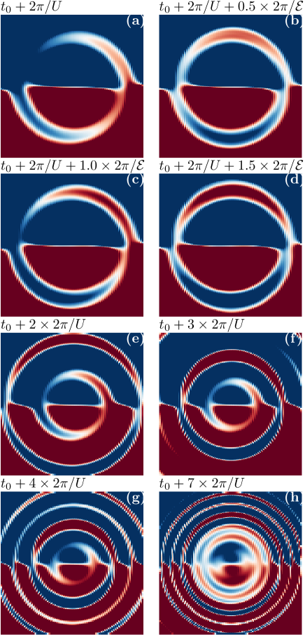
Figure 2: (Color online) False color images of the evolution of the gauge-invariant Wigner distribution in momentum space at different times for ${\mathcal{E}}=2.0$, and $U=0.25$. Each panel shows a snapshot of $n_{\mathbf{k}}(t)$ at an instant in time after the field is switched on (at $t_{0}$). Panels (a) through (d) show the evolution for multiples of the timescale $2\pi/{\mathcal{E}}$ while (e) through (h) show multiples of the timescale $2\pi/U$.

Results.

Prior to the electric field being switched on, the system is in equilibrium at a temperature $T=0.1$ and the Wigner distribution in momentum space is shown in the upper panel of Fig. 1 for $U=0.25$ and is similar for other values of $U$ (but broadened). Vertical cuts through the data are plotted in the lower panel for $V(k)=0$ as a function of $E(k)$ for various values of $U$. Note that despite its similarity to the Fermi-Dirac distribution of a non-interacting system, this result includes the effects of interactions. The shaded area represents the range $[0.45,0.55]$ over which $n_{\mathbf{k}}$ is plotted in the upper panel. This same range is used for all of the following figures, because it is the typical range over which the structures are seen in the long-time behavior. This 10% fluctuation in the signal should be measurable in current experiments.

In the case of a noninteracting system, turning on a static electric field produces Bloch oscillations characterized in frequency space by Wannier-Stark ladders Wannier and in momentum space by periodic oscillations with a period of $2\pi/{\mathcal{E}}$ [Fig. 1(a)]. These Bloch oscillations can be measured in the current or other observables noneq ; MeinertNagerl ; FK_NonEq_DMFT08 ; Kolovsky . The time-evolution of the gauge-invariant Wigner distribution in momentum space is simply the rotation of the equilibrium configuration around the origin like a clock hand with an unchanged Fermi surface shape.

With the interspecies interaction turned on, the Bloch oscillations are gradually damped and decay towards zero. The Joule heating resulting from the interaction increases the energy of the system at a rate given by ${\mathcal{J}}(t)\cdot{\mathcal{E}}$, with ${\mathcal{J}}(t)$ being the light atom current poles . This current eventually decays to zero as the isolated system either thermalizes to an infinite temperature or gets stuck in a nonthermal nonequilibrium steady state. When thermalization occurs, all states are equally occupied and we expect $\lim_{t\to\infty}n_{E,V}=0.5$ for all $(E,V)$ points thermalization . Regardless of the thermalization scenario, the long-time limit is approached with the formation of specific patterns depending on the values of the electric field and the interspecies interaction. Two timescales characterize this development. One is related to the Bloch oscillations, $T_{Bloch}=2\pi/{\mathcal{E}}$ and the other is related to the collapse and revival of the Bloch oscillations for large fields and small interactions, $T_{Beat}=2\pi/U$ MGreinerBlochNature ; MeinertNagerl ; BuchleitnerKolovsky . We focus here on the large-field case ($\mathcal{E}=2$), which has rich behavior that should be detectable in experiments.

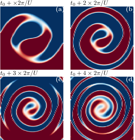
Figure 3: (Color online) False color images of the evolution of the gauge-invariant Wigner distribution in momentum space with time for ${\mathcal{E}}$=2.0 and $U=1.0$. Each panel shows a snapshot of $n_{\mathbf{k}}(t)$ at the corresponding instant in time.

Figure 2 shows different stages of the time evolution of the gauge-invariant Wigner distribution in the $(E,V)$-plane for ${\mathcal{E}}=2.0$, and $U=0.25$. Panels (a) through (d) probe the timescale $T_{Bloch}$ while (e) through (h) probe the timescale $T_{Beat}$. This evolution is characterized by the formation of concentric ring shaped turbulences with a region of high occupation and a region of low occupation that are spawned at the origin, $(E,V)=(0,0)$, and then move outward while at the same time oscillating around this origin (similar to a pebble being dropped into a pond). These turbulences are formed on a time scale of $T_{Beat}$ reminiscent of the beats that are observed in the current as a function of time for large fields and small interaction values as previously illustrated in Ref. FK_NonEq_DMFT08, . While they are moving away from the center, these turbulences also subtly rotate around the origin with a time scale of $T_{Bloch}$. Each new $T_{Beat}$ time interval sees the formation of a new ring at the origin; they eventually pack closer and closer together at long times, making the region more homogeneous. Movies of the evolutions are shown with the supplemental material, where it is easier to see the rotations with period $T_{Bloch}$.

In Fig. 3, the evolution is observed for the same value of the electric field, ${\mathcal{E}}=2.0$ and $U=1.0$. In this case, the formation of the rings, their outward motion away from the origin as well as their oscillation around the center occur on similar time scales. As a result the rings are no longer separated as in the case of smaller interactions. Instead we see the formation of a spiral whose length grows with time (like a dog catching its tail). The spiral grows in length with the addition of a new layer after each $T_{Beat}$ time step in a way analogous to the case of smaller interactions. The central region has a persistent pattern similar to the Yin and Yang symbol in Chinese culture.

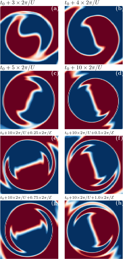
Figure 4: (Color online) False color image of the evolution of the gauge-invariant Wigner distribution with time for ${\mathcal{E}}=2.0$ and $U=3.0$. Panels (a) through (d) show the behavior of the system on the timescale $2\pi/U$ while panels (e) through (h) show the timescale $2\pi/{\mathcal{E}}$.

When the interspecies interaction becomes larger, we see the formation in the middle of the spiral of a feature topologically analogous to the “red spot of Jupiter” with one region of high occupation and one of low occupation (see Fig. 4). The formation of rings is initially reduced to that of small sharp edges on two well defined regions as shown in Fig. 4 (a) through (d). At even longer times, we observe no further changes to this central feature and all the disturbances seem to be taking place outside of the simulated region. Throughout this evolution, the whole system rotates around the origin with a period of $T_{Bloch}$ as seen in Fig. 4 (d) through (h). The size of this “red spot of Jupiter” grows with the interaction so that for even larger $U$, one would see a behavior analogous to the rotating Fermi surface of the noninteracting system at the Bloch frequency.

The evolution of the gauge-invariant Wigner distribution shows the development of patterns that are robust and persistent up to very long times. It is important to note that these patterns are most apparent when one focuses in on a window around the infinite temperature thermal state where $n_{\mathbf{k}}=0.5$. Initially, the Wigner distribution is between 0 and 1 and as the system heats up due to Joule heating, this interval is gradually reduced so that at long times, the high density region and the low density region are shown with Wigner distributions focused between 0.45 and 0.55. Note that the diffraction pattern at the boundaries between different regions is due to the rendering algorithm of the plotting software Paraview and are not physical results.

Conclusion.

We have studied the real-time evolution of the distribution function in momentum space of a field-driven light-heavy Fermi-Fermi mixture of atoms described by the Falicov-Kimball model. This evolution is governed by timescales related to Bloch oscillations and beats in the current through the formation of specific patterns of the distribution function. The system, initially in equilibrium with a distribution function similar to a Fermi-Dirac distribution, evolves through these patterns towards a stationary state where all states are equally occupied [$n_{\mathbf{k}}=0.5$]. For ${\mathcal{E}}=2.0$ and $U=0.25$, we found that the momentum space distribution function develops concentric ring-shaped turbulences around the origin (pebble in the pond). These become a spiral when $U=1.0$ (dog chasing its tail) and for larger $U$, we see the formation of a feature analogous to the “red spot of Jupiter” with a stable region of high occupation and low occupation that rotates around the origin with the Bloch period. Current technology in cold atom experiments should be able to see these features.

Supplemental Material for:
Using an artificial electric field to create the analog of the red spot of Jupiter in light-heavy Fermi-Fermi mixtures of ultracold atoms

Here we provide further details about the numerical calculation of the gauge-invariant Wigner distribution function as well as the production of the corresponding videos.

The nonequilibrium problem is solved on the Kadanoff-Baym-Keldysh contour which is discretized with a spacing $\Delta t$ between consecutive times on the real branch while the imaginary branch has a spacing of $0.1i$ as shown in Fig. 5. The calculation is carried out for different values of $\Delta t$ and then extrapolated using a quadratic extrapolation to $\Delta t=0$.

Figure 5: Kadanoff-Baym-Keldysh contour for the nonequilibrium calculation of the two-time Green’s function.

In dynamical mean-field theory, the self-energy keeps its time dependence but has no momentum dependence. This can be written as:

$$\Sigma_{\mathbf{k}}(t,t^{\prime})=\Sigma(t,t^{\prime}).$$ (1)

The DMFT problem is solved for the two-time contour-ordered Green’s function defined by

$$G^{c}_{\mathbf{k}}(t,t^{\prime})=-i\,{\mathbf{Tr}}\,{\mathcal{T}_{c}}{\mathbf{e}}^{-\beta{\mathcal{H}}_{eq}}c_{\mathbf{k}}(t)c^{\dagger}_{\mathbf{k}}(t^{\prime})/{\mathcal{Z}}_{eq}$$ (2)

with the operators in the Heisenberg representation. To calculate the local contour-ordered Green’s function $G^{c}_{loc}(t,t^{\prime})$, a summation over momentum is necessary. The problem is first mapped onto the two band energies $E(\mathbf{k})$ and $V(\mathbf{k})$, so that the summation is reduced to a double integration. This integral is then calculated with a double Gaussian integration.

The local retarded and the lesser Green’s functions, $G^{R}(t,t^{\prime})$ and $G^{<}(t,t^{\prime})$, are extracted from the local contour ordered Green’s function. The complete description of this solution is given in Ref. FK_NonEq_DMFT08 . In addition, the algorithm also determines the local self-energy. From this, the k-dependent retarded and lesser Green’s functions, $G^{<}_{E({\mathbf{k}}),V({\mathbf{k}})}(t,t^{\prime})$ and $G^{R}_{E({\mathbf{k}}),V({\mathbf{k}})}(t,t^{\prime})$ are constructed by using Dyson’s equation and the momentum-dependent noninteracting Green’s function in the presence of a field.

Note that these Green’s functions are calculated in the vector-potential-only gauge. However, it is the gauge-invariant Wigner distribution jauho that is experimentally measurable. The gauge-invariant Wigner distribution is defined by:

$$n_{E({\mathbf{k}}),V({\mathbf{k}})}(t)=-iG^{<}_{E({\mathbf{k}}+{\mathbf{A}}(t)),V({\mathbf{k}}+{\mathbf{A}}(t))}(t,t),$$ (3)

but we actually calculate it from the ratio

$$n_{E({\mathbf{k}}),V({\mathbf{k}})}(t)=-i\frac{G^{<}_{E({\mathbf{k}}+{\mathbf{A}}(t)),V({\mathbf{k}}+{\mathbf{A}}(t))}(t,t)}{G^{R}_{E({\mathbf{k}}+{\mathbf{A}}(t)),V({\mathbf{k}}+{\mathbf{A}}(t))}(t,t)}$$ (4)

since the equal-time retarded Green’s function is simply the equalt-time anticommutator which is equal to 1. We find this ratio expression to converge faster to the $\Delta t\rightarrow 0$ result, since the retarded Green’s function for a given discretization size often is not precisely equal to 1.

The convergence is generally robust for small interactions and becomes harder for large interactions where a finer time grid is required and where the equilibrium result is difficult to reproduce. Moment sum rules extrapolated to $\Delta t=0$ are used to gauge the accuracy of the final calculations.

To produce the movies of the time evolution of the gauge-invariant Wigner distribution, we use the visualization software paraview Paraview . The distribution function $n_{E({\mathbf{k}}),V({\mathbf{k}})}(t)$ is represented with a false color plot for each time step as a function of $E(\mathbf{k})$ and $V(\mathbf{k})$ producing the corresponding frame. The frames are then linked together to produce a video. A measure of time is given by the horizontal bar at the top of the graph. Initially, it’s orange color indicates elapsed time with the system in equilibrium (no electric field). This is followed by the coloring in green that indicates elapsed time after the electric field is switched on at $t_{0}=5.0$.

For the animations, we used a region of k-space defined by a disk of radius 4 in the $[E(\mathbf{k}),V(\mathbf{k})]$ plane. This choice is due to the fact that the band energy and band velocity will be constrained in a similar way for an experiment in finite dimensions and also that it is visually more compatible with the rotations arising from the electric field.

All the movies presented are for the electric field ${\mathcal{E}}=2.0$. For $U=0.25$, the system can be tracked up to long times (here up to $t=200$) with $\Delta t=0.1$ and no extrapolation. For $U=1.0$, the time evolution is carried out up to $t=40$ and the scaled result for $\Delta t=0.0$ is obtained by quadratically extrapolating the data with $\Delta t=0.066$, $\Delta t=0.05$ and $\Delta t=0.04$. For $U=3.0$, since the equilibrium result is difficult to reproduce, we simply use one frame repeated for times prior to the electric field being switched on. For subsequent times, the data is extrapolated to $\Delta t=0$ using results from $\Delta t=0.033$, $\Delta t=0.025$ and $\Delta t=0.02$. This produces a small jump in the data at $t_{0}=5$

To improve the resolution of the videos, an interpolation is performed for $n(E,V)$ from a grid with spacing $\Delta E=\Delta V=0.1$ to one with $\Delta E=\Delta V=0.025$. This improves the resolution of the images by increasing the pixelation without changing the underlying structure. Note that the rendering algorithim of paraview works by coloring triangulated images, which produces an artificial diffraction effect at some of the boundaries of the images, which is an artifact of this rendering algorithm and not a real effect in the data.

References

- (1) L. M. Falicov and J. C. Kimball, Phys. Rev. Lett. 22, 997 (1969).
- (2) C. Ates and K. Ziegler, Phys. Rev. A 71, 063610 (2005).
- (3) W. Metzner and D. Vollhardt, Phys. Rev. Lett. 62, 324 (1989).
- (4) J. K. Freericks and V. Zlatić, Rev. Mod. Phys. 75, 1333 (2003).
- (5) R. Peierls, Z. Phys. 80, 763 (1933).
- (6) J. K. Freericks, V. M. Turkowski, and V. Zlatić, Phys. Rev. Lett. 97, 266408 (2006).
- (7) J. K. Freericks, Phys. Rev. B 77, 075109 (2008).
- (8) L. P. Kadanoff and G. Baym, Quantum Statistical Mechanics ( Benjamin, New York, 1962).
- (9) L. V. Keldysh, Zh. Eksp. Teor. Fiz. 47, 1945 (1964) [Sov. Phys. JETP 20, 1018 (1964)].
- (10) R. Bertoncini and A. P. Jauho, Phys. Rev. B 44, 3655 (1991).
- (11) G. H. Wannier, Phys. Rev. 100, 1227 (1955); 101, 1835 (1956); 117, 432 (1960); Rev. Mod. Phys. 34, 645 (1962).
- (12) A. R. Kolovsky, Phys. Rev. Lett. 90, 213002 (2003).
- (13) F. Meinert, M. J. Mark, E. Kirilov, K. Lauber, P. Weinmann, M. Gröbner and H.-C. Nägerl, arxiv:1309.4045v1 (2013).
- (14) M. Mierzejewski, J. Bonča, and P. Prelovšek, Phys. Rev. Lett. 107, 126601 (2011).
- (15) H. F. Fotso, K. Mikelsons and J. K. Freericks, Thermalization of driven quantum systems, unpublished.
- (16) M. Greiner, O. Mandel, T. W. Hänsch and I. Bloch, Nature 419, 51 (2002).
- (17) A. Buchleitner and A. R. Kolovsky, Phys. Rev. Lett. 91, 253002 (2003).
- (18) http://www.paraview.org/