Revisionist Integral Deferred Correction with Adaptive Step-Size Control

Abstract

Adaptive step-size control is a critical feature for the robust and efficient numerical solution of initial-value problems in ordinary differential equations. In this paper, we show that adaptive step-size control can be incorporated within a family of parallel time integrators known as Revisionist Integral Deferred Correction (RIDC) methods. The RIDC framework allows for various strategies to implement step-size control, and we report results from exploring a few of them.

Keywords: Initial-value problems, revisionist integral deferred correction, parallel time integrators, local error estimation, adaptive step-size control.

1 Introduction

The purpose of this paper is to show that local error estimation and adaptive step-size control can be incorporated in an effective manner within a family of parallel time integrators based on Revisionist Integral Deferred Correction (RIDC). RIDC methods, introduced in [1], are “parallel-across-the-step” integrators that can be efficiently implemented with multi-core [1, 2], multi-GPGPU [3], and multi-node [4] architectures. The “revisionist” terminology was adopted to highlight that (1) RIDC is a revision of the standard integral defect correction (IDC) formulation [5], and (2) successive corrections, running in parallel but (slightly) lagging in time, revise and improve the approximation to the solution.

RIDC methods have been shown to be effective parallel time-integration methods. They can typically produce a high-order solution in essentially the same amount of wall-clock time as the constituent lower-order methods. In general, for a given amount of wall-clock time, RIDC methods are able to produce a more accurate solution than conventional methods. These results have thus far been demonstrated with constant time steps. It has long been accepted that local error estimation and adaptive step-size control form a critical part of a robust and efficient strategy for solving initial-value problems in ordinary differential equations (ODEs), in particular problems with multiple timescales; see e.g., [6]. Accordingly, in order to assess the practical viability of RIDC methods, it is important to establish whether they can operate effectively with variable step sizes. It turns out that there are subtleties associated with modifying the RIDC framework to incorporate functionality for local error estimation and adaptive step-size control: there are a number of different implementation options, and some of them are more effective than others.

The remainder of this paper is organized as follows. In Section 2, we review the ideas behind RIDC as well as strategies for local error estimation and step-size control. We then combine these ideas to propose various strategies for RIDC methods with error and step-size control. In Section 3, we describe the implementation of these strategies within the RIDC framework and suggest avenues that can be explored for a production-level code. In Section 4, we demonstrate that the use of local error estimation and adaptive step-size control inside RIDC is computationally advantageous. Finally, in Section 5, we summarize the conclusions reached from this investigation and comment on some potential directions for future research.

2 Review of Relevant Background

We are interested in numerical solutions to initial-value problems (IVPs) of the form

$$\left\{\begin{array}[]{l}\displaystyle y^{\prime}(t)=f(t,y(t)),\quad t\in[a,b],\\ \displaystyle y(a)=y_{a}.\end{array}\right.$$ (3)

where $y(t):\mathbb{R}\to\mathbb{R}^{m}$, $y_{a}\in\mathbb{R}^{m}$, and $f:\mathbb{R}\times\mathbb{R}^{m}\to\mathbb{R}^{m}$. We first review RIDC methods, a family of parallel time integrators that can be applied to solve (3). Then, we review strategies for local error estimation and adaptive step-size control for IVP solvers.

2.1 RIDC

RIDC methods [1, 2, 3] are a class of time integrators based on integral deferred correction [5] that can be implemented in parallel via pipelining. RIDC methods first compute an initial (or provisional) solution, typically using a standard low-order scheme, followed by one or more corrections. Each correction revises the current solution and increases its formal order of accuracy. After initial start-up costs, the predictor and all the correctors can be executed in parallel. It has been shown that parallel RIDC methods give almost perfect parallel speedups [1]. In this section, we review RIDC algorithms, generalizing the overall framework slightly to allow for non-uniform step-sizes on the different correction levels.

We denote the nodes for correction level $\ell$ by

$$a=t_{0}^{[\ell]}<t_{1}^{[\ell]}<\cdots<t_{N^{[\ell]}}^{[\ell]}=b,$$

where $N^{[\ell]}$ denotes the number of time steps on the level $\ell$. In practice, the nodes on each level are obtained dynamically by the step-size controller.

2.1.1 The Predictor

To generate a provisional solution, a low-order integrator is applied to solve the IVP (3). For example, a first-order forward Euler integrator applied to (3) gives

$$\eta^{[0]}_{n}=\eta^{[0]}_{n-1}+\left(t_{n}^{[0]}-t_{n-1}^{[0]}\right)f(t_{n-1}^{[0]},\eta^{[0]}_{n-1}),$$ (4)

for $n=1,2,\ldots,N^{[0]}$, with $\eta_{0}^{[0]}=y_{a}$, and where we have indexed the prediction level as level $0$. We denote $\eta^{[\ell]}(t)$ as a continuous extension [6] of the numerical solution at level $\ell$, i.e., a piecewise polynomial $\eta^{[0]}(t)$ that satisfies

$$\eta^{[0]}(t_{n}^{[0]})=\eta_{n}^{[0]}.$$

The continuous extension of a numerical solution is often of the same order of accuracy as the underlying discrete solution [6]. Indeed, for the purposes of this study, we assume $\eta^{[\ell]}(t)$ is of the same order as $\eta^{[\ell]}_{n}$.

2.1.2 The Correctors

Suppose an approximate solution $\eta(t)$ to IVP (3) is computed. Denote the exact solution by $y(t)$. Then, the error of the approximate solution is $e(t)=y(t)-\eta(t)$. If we define the defect as $\delta(t)=f(t,\eta(t))-\eta^{\prime}(t)$, then

$$e^{\prime}(t)=y^{\prime}(t)-\eta^{\prime}(t)=f(t,\eta(t)+e(t))-f(t,\eta(t))+\delta(t).$$

The error equation can be written in the form

$$\left[e(t)-\int_{a}^{t}\delta(\tau)\,d\tau\right]^{\prime}=f\left(t,\eta(t)+e(t)\right)-f\left(t,\eta(t)\right)$$ (5)

subject to the initial condition $e(a)=0$. In RIDC, the corrector at level $\ell$ solves for the error $e^{[\ell-1]}(t)$ of the solution $\eta^{[\ell-1]}(t)$ at the previous level to generate the corrected solution $\eta^{[\ell]}(t)$,

$$\eta^{[\ell]}(t)=\eta^{[\ell-1]}(t)+e^{[\ell-1]}(t).$$

For example, a corrector at level $\ell$ that corrects $\eta^{[\ell-1]}(t)$ by applying a first-order forward Euler integrator to the error equation (5) takes the form

$$e^{[\ell-1]}(t_{n}^{[\ell]})-e^{[\ell-1]}(t_{n-1}^{[\ell]})-\int_{t_{n-1}^{[\ell]}}^{t_{n}^{[\ell]}}\delta^{[\ell-1]}(\tau)\,d\tau=\\ \Delta t_{n}^{[\ell]}\left[f\left(t_{n-1}^{[\ell]},\eta^{[\ell-1]}(t_{n-1}^{[\ell]})+e^{[\ell-1]}(t_{n-1}^{[\ell]})\right)-f\left(t_{n-1}^{[\ell]},\eta^{[\ell-1]}(t_{n-1}^{[\ell]})\right)\right],$$

where $\Delta t_{n}^{[\ell]}=t_{n}^{[\ell]}-t_{n-1}^{[\ell]}$. After some algebraic manipulation, one obtains

$$\eta^{[\ell]}_{n}=\, \eta^{[\ell]}_{n-1}+\Delta t_{n}^{[\ell]}\left(f\left(t_{n-1}^{[\ell]},\eta^{[\ell]}(t_{n-1}^{[\ell]})\right)-f\left(t_{n-1}^{[\ell]},\eta^{[\ell-1]}(t_{n-1}^{[\ell]})\right)\right)$$ (6)

$$+\int_{t_{n-1}^{[\ell]}}^{t_{n}^{[\ell]}}f\left(\tau,\eta^{[\ell-1]}(\tau)\right)\,d\tau.$$

The integral in equation (6) is approximated using quadrature,

$$\int_{t_{n-1}^{[\ell]}}^{t_{n}^{[\ell]}}f\left(\tau,\eta^{[\ell-1]}(\tau)\right)\,d\tau\approx\sum_{i=1}^{|\vec{\mathcal{T}}^{[\ell]}_{n}|}\alpha_{n,i}^{[\ell-1]}f\left(\tau_{i},\eta^{[\ell-1]}(\tau_{i})\right),\quad\tau_{i}\in\vec{\mathcal{T}}^{[\ell]}_{n},$$ (7)

where the set of quadrature nodes, $\vec{\mathcal{T}}^{[\ell]}_{n}$, for a first-order corrector satisfies

1. $|\vec{\mathcal{T}}^{[\ell]}_{n}|=\ell+1$

2. $\vec{\mathcal{T}}^{[\ell]}_{n}\subseteq\{t_{n}^{[\ell-1]}\}_{n=0}^{N^{[\ell-1]}}$

3. $\min(\vec{\mathcal{T}}^{[\ell]}_{n})\leq t_{n-1}^{[\ell]}$

4. $\max(\vec{\mathcal{T}}^{[\ell]}_{n})\geq t_{n}^{[\ell]}$

The quadrature weights, $\alpha_{n,i}^{[\ell-1]}$, are found by integrating the interpolating Lagrange polynomials exactly,

$$\alpha_{n,i}^{[\ell-1]}=\prod_{j=1,j\neq i}^{|\vec{\mathcal{T}}^{[\ell]}_{n}|}\int_{t_{n-1}^{[\ell]}}^{t_{n}^{[\ell]}}\frac{(t-\tau_{j})}{(\tau_{i}-\tau_{j})}\,dt,\quad\tau_{i}\in\vec{\mathcal{T}}^{[\ell]}_{n}.$$ (8)

The term $f\left(t_{n-1}^{[\ell]},\eta^{[\ell-1]}(t_{n-1}^{[\ell]})\right)$ in equation (6) is approximated using Lagrange interpolation,

$$f\left(t_{n-1}^{[\ell]},\eta^{[\ell-1]}(t_{n-1}^{[\ell]})\right)\approx\sum_{i=1}^{|\vec{\mathcal{T}}^{[\ell]}_{n}|}\gamma_{n,i}^{[\ell-1]}f\left(\tau_{i},\eta^{[\ell-1]}(\tau_{i})\right),\quad\tau_{i}\in\vec{\mathcal{T}}^{[\ell]}_{n},$$ (9)

where the same set of nodes, $\vec{\mathcal{T}}^{[\ell]}_{n}$, for the quadrature is used for the interpolation. The interpolation weights are given by

$$\gamma_{n,i}^{[\ell-1]}=\prod_{j=1,j\neq i}^{|\vec{\mathcal{T}}^{[\ell]}_{n}|}\frac{(t_{n-1}^{[\ell]}-\tau_{j})}{(\tau_{i}-\tau_{j})},\quad\tau_{i}\in\vec{\mathcal{T}}^{[\ell]}_{n}.$$ (10)

2.2 Adaptive Step-Size Control

Adaptive step-size control is typically used to achieve a user-specified error tolerance with minimal computational effort by varying the step-sizes used by an IVP integrator. This is commonly done based on a local error estimate. It may also be desirable that the step-size vary smoothly over the course of the integration. We review common techniques for estimating the local error, followed by algorithms for optimal step-size selection.

2.2.1 Error Estimators

Two common approaches for estimating the local truncation error of a single-step IVP solver are through the use of Richardson extrapolation (commonly used within a step-size selection framework known as step-doubling) and embedded Runge–Kutta pairs [6]. Step-doubling is perhaps the more intuitive technique. The solution after each step is estimated twice: once as a full step and once as two half steps. The difference between the two numerical estimates gives an estimate of the truncation error. For example, denoting the exact solution to IVP (3) at time $t_{n}+\Delta t$ as $y(t_{n}+\Delta t)$, the forward Euler step starting from the exact solution at time $t_{n}$ and using a step size of size $\Delta t$ is

$$\eta_{1,n+1}=y(t_{n})+\Delta t\,f(t_{n},y_{n}),$$

and the forward Euler step using two steps of size $\frac{\Delta t}{2}$ is

$$\eta_{2,n+1}=\left(y(t_{n})+\frac{\Delta t}{2}\,f(t_{n},y_{n})\right)+\frac{\Delta t}{2}f\left(t_{n}+\frac{\Delta t}{2},y(t_{n})+\frac{\Delta t}{2}\,f(t_{n},y_{n})\right).$$

Because forward Euler is a first-order method (and thus has a local truncation error of $\mathcal{O}(\Delta t^{2})$), the two numerical approximations satisfy

$$y(t_{n}+\Delta t) =\eta_{1,n+1}+(\Delta t)^{2}\phi+\mathcal{O}(\Delta t^{3})+\cdots,$$

$$y(t_{n}+\Delta t) =\eta_{2,n+1}+2\left(\frac{\Delta t}{2}\right)^{2}\phi+\mathcal{O}(\Delta t^{3})+\cdots,$$

where a Taylor series expansion gives that $\phi$ is a constant proportional to $y^{\prime\prime}(t_{n})$. The difference between the two numerical approximations gives an estimate for the local truncation error of $\eta_{2,n+1}$,

$$e_{n+1}=\eta_{2,n+1}-\eta_{1,n+1}=\frac{\Delta t^{2}}{2}\phi+\mathcal{O}(\Delta t^{3}).$$

An alternative approach to estimating the local truncation error is to use embedded RK pairs [7]. An $s$-stage Runge–Kutta method is a single-step method that takes the form

$$\eta_{n+1} =\eta_{n}+\Delta t\sum_{i=1}^{s}b_{i}k_{i},$$

$$\text{where}\qquad\qquad\ k_{i} =f\left(t_{i}+c_{i}h,\eta_{n}+\Delta t\sum_{j=1}^{s}a_{ij}k_{j}\right),\quad i=1,2,\ldots,s.$$

The idea is to find two single-step RK methods, typically one with order $p$ and the other with order $p-1$, that share most (if not all) of their stages but have different quadrature weights. This is represented compactly in the extended Butcher tableau

$$\begin{array}[]{l|c}c&A\\ \hline\cr&b\\ &\hat{b}\end{array}$$

Denoting the solution from the order-$p$ method as

$$\eta^{*}_{n+1}=\eta_{n}+\Delta t\sum_{i=1}^{s}\hat{b}_{i}k_{i},$$ (11a)

and the solution from the order-$$(p-1)$$ method as

$$\eta_{n+1}=\eta_{n}+\Delta t\sum_{i=1}^{s}b_{i}k_{i},$$ (11b)

the error estimate is

$$e_{n+1}=\eta_{n+1}-\eta^{*}_{n+1}=\Delta t\sum_{i=1}^{s}(b_{i}-\hat{b}_{i})k_{i},$$ (11c)

which is $\mathcal{O}(\Delta t^{p})$.

A third approach for approximating the local truncation error is possible within the deferred correction framework. We observe that that in solving the error equation (5), one is in fact obtaining an approximation to the error. As discussed in Section 3.3, it can be shown that the approximate error after $\ell$ first-order corrections satisfies $o(\Delta t^{p_{0}+\ell+1})$. We shall see in Section 3.3 that this error estimate proves to be a poor choice for optimal step size selection because in our formulation the time step selection for level $\ell$ does not allow for the refinement of time steps at earlier levels.

2.2.2 Optimal Step-Size Selection

Given an error estimate from Section 2.2.1 for a step $\Delta t$, one would like to either accept or reject the step based on the error estimate and then estimate an optimal step-size for the next time step or retry the current step. Following [8], Algorithm 1 outlines optimal step-size selection given an estimate of the local truncation error. In lines 1–4, one computes a scaled error estimate. In line 5, an optimal time step is computed by scaling the current time step. In lines 6–10, a new time step is suggested; a more conservative step-size is suggested if the previous step was rejected.

Input:

$y_{n}$: approximate solution at time $t_{n}$;

$y_{n+1}$: approximate solution at time $t_{n+1}$;

$e_{n+1}$: error estimate for $y_{n+1}$;

$p$: order of integrator;

$m$: number of ODEs;

atol, rtol: user specified tolerances;

prev_rej: flag that indicates whether the previous step was rejected;

$\alpha<1$: safety factor;

$\beta>1$: allowable change in step-size.

Output:

accept_flag: flag to accept or reject this step;

$\Delta t_{new}$: optimal time step

Set $a(i)=\max\{|y_{n}(i)|,|y_{n+1}(i)|\},\,i=1,2,\ldots,m$.

Compute $\tau(i)={\tt atol}+{\tt rtol}*a(i),\,i=1,2,\ldots,m$.

Compute $\epsilon=\sqrt{\frac{\sum_{i=1}^{m}(e(i)/\tau(i))^{2}}{m}}$.

Compute $\Delta t_{opt}=\Delta t\,(\frac{1}{\epsilon})^{1/(p+1)}$.

if prev_rej then

       $\Delta t_{new}=\alpha\min\{\Delta t,\max\{\Delta t_{opt},\Delta t/\beta\}\}$

else

       $\Delta t_{new}=\alpha\min\{\beta\Delta t,\max\{\Delta t_{opt},\Delta t/\beta\}\}$

end if

if $\epsilon>1$ then

       ${\tt accept\_flag}=1$

else

       ${\tt accept\_flag}=0$

end if

Algorithm 1 Optimal step-size selection algorithm. The approximate solution, the error estimate, and its order are provided as inputs. For the numerical experiments in Section 4, we fix $\alpha=0.9$, $\beta=10$.

3 RIDC with Adaptive Step-Size Control

There are numerous adaptive step-size control strategies that can be implemented within the RIDC framework. We consider three of them in this paper as well as discuss other strategies that are possible.

3.1 Adaptive Step-Size Control: Prediction Level Only

One simple approach to step-size control with RIDC is to perform adaptive step-size control on the prediction level only, for example using step-doubling or embedded RK pairs as error estimators for the step-size control strategy. The subsequent correctors then use this grid unchanged (i.e., without performing further step-size control). With this strategy, corrector $\ell$ is lagged behind corrector $\ell-1$ so that each node simultaneously computes an update on its level (after an initial startup period). This is illustrated graphically in Figure 1. In principle, parallel speedup is maintained with this approach, and a minimal memory footprint is required in an implementation. Additionally, an interpolation step is circumvented because the nodes are the same on each level. There are however a few potential drawbacks in this approach. First, it is not clear how to distribute the user-defined tolerance among the levels. Clearly, satisfying the user-specified tolerance on the prediction level defeats the purpose of the deferred correction approach. Estimating a reduced tolerance criterion may be possible a priori, but such an estimate would at present be ad hoc. Second, there is no reason to expect the corrector (6) should take the same steps to satisfy an error tolerance when computing a numerical approximation to the error equation (5).

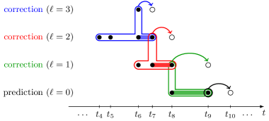
Figure 1: Schematic diagram of step-size control on the prediction level only. The filled circles denote previously computed and stored solution values at particular times. The corrections are run in parallel (but lagging in time) and the open circles indicate which values are being simultaneously computed. The stencil of points required by each level is shown by the “bubbles” surrounding certain grid points; the thick horizontal shading indicates the integrals needed in (6). Note each level uses the same grid in time.

3.2 Adaptive Step-Size Control: All Levels

A generalization of the above formulation is to utilize adaptive step-size control to solve the error equations (5) as well. The variant we consider is step-doubling on all levels, where each predictor and corrector performs Algorithm 1; embedded RK pairs can also be used to estimate the error for step-size adaptivity on all levels. Intuitively, step-size control on every level gives more opportunity to detect and adapt to error than simply adapting using the (lowest-order) predictor. For example, this allows the corrector take a smaller step if necessary to satisfy an error tolerance when solving the error equation. Some drawbacks are: (i) an interpolation step is necessary because the nodes are generally no longer in the same locations on each level, (ii) more memory registers are required, and (iii) there is a potential loss of parallel efficiency because a corrector may be stalled waiting for an adequate stencil to become available to compute a quadrature approximation to the integral in equation (6). Another issue — both a potential benefit and a potential drawback — is the number of parameters that can be tuned for each problem. A discussion on the effect of tolerance choices for each level is provided in Section 4. One can in practice also tune step-size control parameters $\alpha,\beta$, atol, and rtol for Algorithm 1 separately on each level. Figure 2 highlights that some nodes might not be able to compute an updated solution on their current level if an adequate stencil is not available to approximate the integral in equation (6) using quadrature. In this example, the level $\ell=2$ correction is unable to proceed, whereas the prediction level $\ell=0$ and corrections $\ell=1$ and $\ell=3$ are all able to advance the solution by one step.

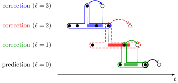
Figure 2: Schematic diagram of a scenario when step-size control is applied on all levels. Unlike in Figure 1, here each level has its own grid in time. Solid circles indicate particular times and levels where the solution is known. In this particular diagram, levels $\ell=0,1,3$ are all able to advance simultaneously to the open circles. However, correction level $\ell=2$ is unable to advance to the time indicated by the triangle symbol because correction level $\ell=1$ has not yet computed far enough. The stencil of points required by each level is shown by the “bubbles” surrounding certain grid points; the thick horizontal shading indicates the integrals needed in (6). Note in particular that the dashed stencil includes a open circle at level $\ell=1$ that is not yet computed.

3.3 Adaptive Step-Size Control: Using the Error Equation

A third strategy one might consider is adaptive step-size control for the error equation (5) using the solution to the error equation itself as the error estimate. (One still uses step-doubling or embedded RK pairs to obtain an error estimate for step-size control on the predictor equation (3)). At first glance, this looks promising provided the order of the integrator can be established because it is used to determine an optimal step-size. One would expect computational savings from utilizing available error information, as opposed to estimating it via step-doubling or an embedded RK pair.

If first-order predictor and first-order correctors are used to construct the RIDC method, the analysis in [9] can be easily extended to the proposed RIDC methods with adaptive step-size control. We note that the numerical quadrature approximation given in equation (7) and the numerical interpolation given in equation (9) are accurate to the order $\mathcal{O}(\Delta t_{n}^{\ell+2})$; this is sufficient for the inductive proof in [9] to hold. Hence, one can show that the method has a formal order of accuracy $\mathcal{O}(\Delta t^{\ell+2})$, where $\Delta t=\max_{n,\ell}(t_{n}^{[\ell]}-t_{n-1}^{[\ell]})$.

Although the formal order of accuracy can be established, using the error estimate from successive levels is a poor choice for optimal step-size selection. Consider step-size selection for level $\ell$, time step $t_{n}^{[\ell]}$, using $\eta_{n}^{[\ell]}-\eta^{[\ell-1]}(t_{n}^{[\ell]})$ as the error estimator in Algorithm 1. The optimal step-size is chosen to control the local error estimate via the step-size $\Delta t_{n}^{[\ell]}=t_{n}^{[\ell]}-t_{n-1}^{[\ell]}$. However, the local error for the correctors generally contains contributions from the solutions at all the previous levels. The validity of the asymptotic local error expansion of the RIDC method in terms of $\Delta t_{n}^{[\ell]}$ requires that $\Delta t=\max_{n,\ell}(t_{n}^{[\ell]}-t_{n-1}^{[\ell]})$ be sufficiently small, and it is not normally possible to guarantee this in the context of an IVP solver. In other words, the step-size controller for a corrector at a given level cannot control the entire local error, and hence standard step-control strategies, which are predicated on the validity of error expansions in terms of only the step-size to be taken, cannot be expected to perform well. We present some numerical tests in Section 4.2.4 to illustrate the difficulties with using successive errors as the basis for step-size control.

3.4 Further Discussion

There are many other strategies/implementation choices that affect the overall performance of the adaptive RIDC algorithm. Some have already been discussed in the previous section. We summarize some of the implementation choices that must be made:

• The choice of how to estimate the error of the discretization must be made. Three possibilities have already been mentioned: step-doubling, embedded RK pairs, and solutions to the error equation (5). A combination of all three is also possible.

• If an IVP method with adaptive step-size control is used to solve equation (5), choices must be made as to how the tolerances and step-size control parameters, $\alpha$ and $\beta$, are to be chosen for each correction level.

We also list a few implementation details that should be considered when designing adaptive RIDC schemes.

• If adaptive step-size control is implemented on all levels, some correction levels may sit idle because the information required to perform the quadrature and interpolation in (6) is not available. This idle time adversely affects the parallel efficiency of the algorithm. One possibility to decrease this idle time is instead of taking an “optimal step” (as suggested by the step-size control routine), one could take a smaller step for which the quadrature and interpolation stencil is available. There is some flexibility in choosing exactly which points are used in the quadrature stencil, and it might also be possible to choose a stencil to minimize the time that correction levels are sitting idle.

• Because values are needed from lower-order correction levels, the storage required by a RIDC scheme depends on when values can be overwritten (see, e.g., the stencils in Figures 1 and 2). Thus to avoid increasing the storage requirements, the prediction level and each correction level should not be allowed to get too far ahead of higher correction levels. Although this is also the case for the non-adaptive RIDC schemes [1, 2], if adaptive step-size control is implemented on all levels (Figure 2), the memory footprint is likely to increase. Some consideration should thus be given to a potential trade-off between parallel efficiency and the overall memory footprint of the scheme.

• It is important to reduce round-off error when computing the quadrature weights (8) and the interpolation weights (10). This can be done by through careful scaling and control of the order of the floating-point operations [10].

• If one wishes to use higher-order correctors and predictors to construct RIDC integrators, we note that the convergence analysis in [11, 12, 13] only holds for uniform steps. A non-uniform mesh introduces discrete “roughness” (see [12]); hence, an increase of only one order per correction level is guaranteed even though a high-order method is used to solve equation (5).

Additionally, the RIDC framework, by construction, solves a series of error equations to generate a successively more accurate solution. This framework can be potentially be exploited to generate order-adaptive RIDC methods. For example, one might control the number of corrector levels adaptively based on an error estimate.

4 Numerical Examples

We focus on the solutions to three nonlinear IVPs. The first is presented in [14]; we refer to it as the Auzinger IVP:

$$\left\{\begin{array}[]{l}\displaystyle\vspace*{1mm}y_{1}^{\prime}=-y_{2}+y_{1}(1-y_{1}^{2}-y_{2}^{2}),\\ \vspace*{1mm}\displaystyle y_{2}^{\prime}=y_{1}+3y_{2}(1-y_{1}^{2}-y_{2}^{2}),\\ \displaystyle y(0)=(1,0)^{T},\quad t\in[0,10],\\ \end{array}\right.$$ (15)

that has the analytic solution $y(t)=(\cos{t},\sin{t})^{T}$.

The second is the IVP associated with the Lorenz attractor:

$$\left\{\begin{array}[]{l}\displaystyle\vspace*{1mm}y_{1}^{\prime}=\sigma(y_{2}-y_{1}),\\ y_{2}^{\prime}=\rho y_{1}-y_{2}-y_{1}y_{3},\\ \vspace*{1mm}y_{3}^{\prime}=y_{1}y_{2}-\beta y_{3},\\ y(0)=(1,1,1)^{T},\quad t\in[0,1].\end{array}\right.$$ (20)

For the parameter settings $\sigma=10,\ \rho=28,\ \beta=8/3$, this system is highly sensitive to perturbations, and an IVP integrator with adaptive step-size control may be advantageous.

The third is the restricted three-body problem from [6]; we refer to it as the Orbit IVP:

$$\left\{\begin{array}[]{l}\displaystyle\vspace*{1mm}\displaystyle y_{1}^{\prime\prime}=y_{1}+2y_{2}^{\prime}-\mu^{\prime}\frac{y_{1}+\mu}{D_{1}}-\mu\frac{y_{1}-\mu^{\prime}}{D_{2}}\\ \vspace*{1mm}\displaystyle y_{2}^{\prime\prime}=y_{2}-2y_{1}^{\prime}-\mu^{\prime}\frac{y_{2}}{D_{1}}-\mu\frac{y_{2}}{D_{2}}\\ \vspace*{1mm}\displaystyle D_{1}=\left((y_{1}+\mu)^{2}+y_{2}^{2}\right)^{3/2},\quad D_{2}=\left((y_{1}-\mu^{\prime})^{2}+y_{2}^{2}\right)^{3/2},\\ \displaystyle\mu=0.012277471,\quad\mu^{\prime}=1-\mu.\end{array}\right.$$ (25)

Choosing the initial conditions

$$y_{1}(0)=0.994,\quad y_{1}^{\prime}(0)=0,\quad y_{2}(0)=0,$$

$$y_{2}^{\prime}(0)=-2.00158510637908252240537862224,$$

gives a periodic solution with period $t_{end}=17.065216560159625588917206249$.

We now present numerical evidence to demonstrate that:

1. RIDC integrators with non-uniform step-sizes converge and achieve their designed orders of accuracy.

2. RIDC methods with adaptive step-size based on step-doubling and embedded RK error estimators, on the prediction level only, converge.

3. RIDC methods with adaptive step-size control based on step-doubling to estimate the local error on the prediction and correction levels converge; however, the step-sizes selected are poor (many rejected steps), even for the smooth Auzinger problem.

4. RIDC methods with adaptive step-size control based on step-doubling to estimate the local error on the prediction level but using the solution to the error equation for step-size control results is problematic.

4.1 RIDC with non-uniform step-sizes

For our first numerical experiment, we demonstrate that RIDC integrators with non-uniform step-sizes converge and achieve their design orders of accuracy. Figure 3 shows the classical convergence study (error as a function of mean step-size) for the RIDC integrator applied to equation (15). Figure 3(a) shows the convergence of RIDC integrators with uniform step-sizes; Figures 3(b)–(d) show the convergence of RIDC integrators when random step-sizes are chosen. The random step-sizes are chosen so that

$$\Delta t_{n}^{[\ell]}\in\left[\frac{1}{\omega}\Delta t_{n-1}^{[\ell]},\omega\Delta t_{n-1}^{[\ell]}\right],\quad\omega\in\mathbb{R},$$

where $\omega$ controls how rapidly a step-size is allowed to change. The figures show that RIDC integrators with non-uniform step-sizes achieve their designed order of accuracy (each additional correction improves the order of accuracy by one), at least up to order 6. In Figure 3 (corresponding to RIDC with uniform step-sizes), we observe that the error stagnates at a value significantly larger than machine precision. This is likely due to numerical issues associated with quadrature on equispaced nodes [15]. We note that $\omega=1$ gives the uniformly distributed case. We also observe that as the ratio of the largest to the smallest cell increases, the performance of higher-order RIDC methods degrades, likely due to round-off error associated with calculating the quadrature and interpolation weights.

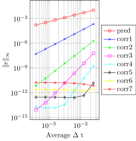
(a) Uniform steps

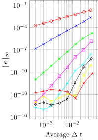
(b) Random steps, $\omega=2$

(c) Random steps, $\omega=4$

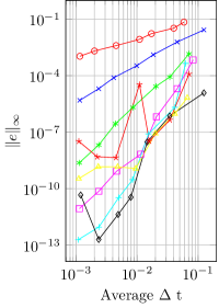
(d) Random steps, $\omega=100$

Figure 3: Auzinger IVP: The design order is illustrated for the RIDC methods.

Figure 4 shows the convergence study (error as a function of mean step-size) for equation (20). The reference solution is computed using an RK-45 integrator with a fine time step. Similar observations can be made that RIDC methods with non-uniform step-sizes converge with their designed orders of accuracy (at least up to order 6).

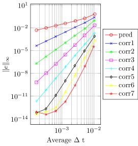
(a) Ratio = 1 (uniform)

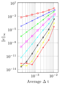
(b) Ratio = 2

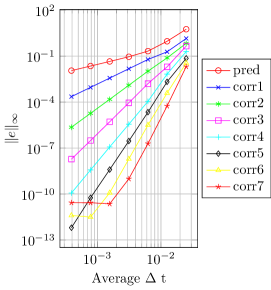
(c) Ratio = 4

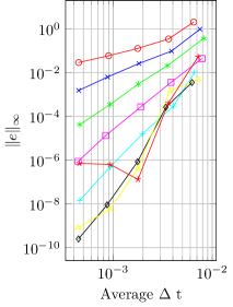
(d) Ratio = 100

Figure 4: Lorenz IVP: The design order is illustrated for the RIDC methods.

4.2 Adaptive RIDC

We study four different variants of RIDC methods with adaptive step-size control: (i) step-doubling is used for adaptive step-size control on the prediction level only (Section 4.2.1); (ii) an embedded RK pair is used for adaptive step-size control on the prediction level only (Section 4.2.2); (iii) step-doubling is used for adaptive step-size control on the prediction and correction levels (Section 4.2.3); and (iv) step-doubling is used for adaptive step-size control on the prediction level, and the computed errors from the error equation (5) are used for adaptive step-size control on the correction levels.

4.2.1 Step-Doubling on the Prediction Level Only

In this numerical experiment, we solve the orbit problem (25) using a fourth-order RIDC method (constructed using forward Euler integrators), and adaptive step-size control on the prediction level only, where step-doubling is used to provide the error estimate. As shown in Figure 5, successive correction loops are able to reduce the error in the solution and recover the desired orbit. The red circles in Figure 5a indicate rejected steps.

(a) prediction

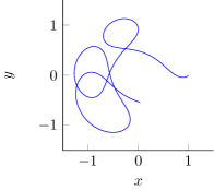
(b) 1^st Correction

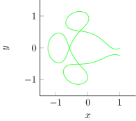
(c) 2^nd Correction

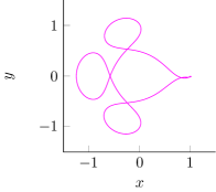
(d) 3^rd Correction

Figure 5: Orbit problem: Although the prediction level gives a highly inaccurate solution, successive correction loops are able to reduce the error and produce the desired orbit. The red circles on the prediction level (a) indicate rejected steps.

Figure 6a shows that RIDC with step-doubling only on the prediction level converges as the tolerance is reduced. In this experiment, the RIDC integrator is reset after every 100 accepted steps. By “reset” [1], we mean that the highest-order solution after every 100 steps is used as an initial condition to re-initialize the provisional solution; e.g., instead of solving equation (3), one solves a sequence of problems

$$\left\{\begin{array}[]{l}\displaystyle y^{\prime}(t)=f(t,y),\quad t\in[t_{100},\min(b,t_{200})],\\ \displaystyle y(t_{100i})=\eta_{100(i-1)}^{[P-1]}.\end{array}\right.$$

if $(L-1)$ correctors are applied and $\eta_{0}^{[L-1]}=y_{a}$. The time steps chosen by the RIDC integrator with resets performed every 100 and 400 steps are shown in Figures 6b and 6c.

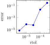
(a) Convergence study

rtol	atol	error	naccept	nreject
$10^{-3.5}$	$10^{-6.5}$	2.72e–01	1456	99
$10^{-4.0}$	$10^{-7.0}$	2.08e–02	2650	81
$10^{-4.5}$	$10^{-7.5}$	5.35e–05	4730	68
$10^{-5.0}$	$10^{-8.0}$	7.39e–05	8436	42
$10^{-5.5}$	$10^{-8.5}$	6.72e–06	15031	10

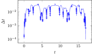
(b) Adaptive step-sizes selected (reset every 100 steps)

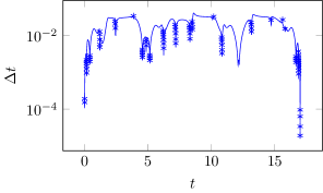
(c) Adaptive step-sizes selected (reset every 400 steps)

Figure 6: Orbit Problem: (a) Convergence of a fourth-order RIDC method constructed with forward Euler integrators and adaptive step-size control on the prediction level (using step-doubling). Convergence is measured relative to the exact solution as the tolerance is decreased. A reset is performed after every 100 accepted steps for this convergence study. In (b), the step-sizes selected for rtol = $10^{-3.5}$ and atol = $10^{-6.5}$ are displayed as the solid curve and rejected steps as “x”s; a reset is performed after every 100 steps. In (c), the reset is performed after every 400 steps. Observe that although the number of rejected steps increases, the overall $\Delta t$ chosen remains qualitatively similar.

In Figure 6b, $\Delta t_{min}=1.06\times 10^{-4}$. If a non-adaptive fourth-order RIDC method was used with $\Delta t_{min}$, 160814 uniform time steps would have been required. By adaptively selecting the time steps for this example and tolerance, the adaptive RIDC method required approximately one one-hundredth of the functional evaluations, corresponding to a one hundred-fold speedup.

4.2.2 Embedded RK on the Prediction Level Only

In this numerical experiment, we repeat the orbit problem (25) using a fourth-order RIDC method constructed again using forward Euler integrators, but the step-size adaptivity on the prediction level uses a Heun–Euler embedded RK pair. This simple scheme combines Heun’s method, which is second order, with the forward Euler method, which is first order. Figure 7a shows the convergence of this adaptive RIDC method as the tolerance is reduced. As the previous example, the RIDC integrator is reset after every 100 accepted steps for the convergence study. In Figures 7b and 7c, we show the time steps chosen by the RIDC integrator with resets performed after 100 or 400 steps, respectively.

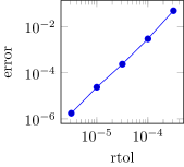
(a) Convergence study

rtol	atol	error	naccept	nreject
$10^{-3.5}$	$10^{-6.5}$	4.91e–02	2082	93
$10^{-4.0}$	$10^{-7.0}$	2.96e–03	3754	71
$10^{-4.5}$	$10^{-7.5}$	2.36e–04	6703	50
$10^{-5.0}$	$10^{-8.0}$	2.28e–05	11945	20
$10^{-5.5}$	$10^{-8.5}$	1.77e–06	21277	10

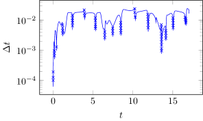
(b) Adaptive step-sizes selected (reset every 100 steps)

(c) Adaptive step-sizes selected (reset every 400 steps)

Figure 7: Orbit Problem: (a) Convergence of a fourth-order RIDC method constructed with forward Euler integrators and adaptive step-size control on the prediction level (using an embedded RK pair to estimate the error). Convergence is measured relative to the exact solution as the tolerance is decreased. A reset is performed after every 100 accepted steps for this convergence study. In (b), the step-sizes selected for rtol = $10^{-3.5}$ and atol = $10^{-6.5}$ are displayed as the solid curve and rejected steps as “x”s; a reset is performed after every 100 steps. In (c), the reset is performed after every 400 steps.

Not surprisingly, the time steps chosen by the RIDC method are dependent on the specified tolerances and the error estimator (and consequently the integrators used to obtain a provisional solution to (3)) used for the control strategy. One can easily construct a RIDC integrator using higher-order embedded RK pairs to solve for a provisional solution to (3), and then use the forward Euler method to solve the error equation (5) on subsequent levels. For example, Figure 8 shows the step sizes chosen when the Bogacki–Shampine method [16] (a 3(2) embedded RK pair) and the popular Runge–Kutta–Fehlberg 4(5) pair [17] is used to compute the provisional solution (and error estimate) for the RIDC integrator. The same tolerance of rtol = $10^{-3.5}$ is used to generate both graphs. As the order and accuracy of the predictor increases, one can take larger time steps. For this example, using higher-order embedded RK pairs as step-size control mechanisms for RIDC methods result in less variations in time steps.

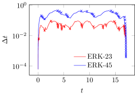
Figure 8: Step-sizes selected by RIDC methods constructed using a Bogacki–Shampine method, a 3(2) embedded pair (red) and the Runge–Kutta-Fehlberg 4(5) pair. ’x’ indicates rejected steps.

4.2.3 Step-Doubling on All Levels

As mentioned in Subsection 3.2, it might be advantageous to use adaptive step-size control when solving the error equations. This affords a myriad of parameters that can be used to tune the step-size control mechanism. In this set of numerical experiments, we explore how the choice of tolerances for the prediction/correction levels affect the step-size selection.

We first solve the Auzinger IVP using step-doubling on all the levels, i.e., both predictor and corrector levels. In Figure 9, we show the computed step-sizes when we naively choose the same tolerances on each level. As expected, the predictor has to take many steps (to satisfy the stringent user-supplied tolerance), whereas life is easy for the correctors. In principle, the correctors are not even needed. Equally important to note is that the error increases after the last correction loop. This might seem surprising at first glance but ultimately may not unreasonable because the steps selected to solve the third correction are not based on the solution to the error equation but rather the original IVP.

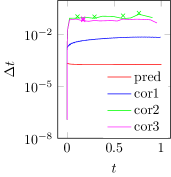
$\ell$	rtol	atol	error	naccept	nreject
0	$10^{-8}$	$10^{-10}$	2.028e–05	5480	0
1	$10^{-8}$	$10^{-10}$	8.824e–07	197	0
2	$10^{-8}$	$10^{-10}$	1.917e–08	19	4
3	$10^{-8}$	$10^{-10}$	6.386e–07	25	2

Figure 9: Auzinger IVP: step-size control is implemented on all prediction and correction levels. The same tolerances are used for each level. As expected, the predictor has a hard time (forward Euler must satisfy a stringent tolerance); on the other hand, life is easy for the correctors. ’x’ in the figure indicate the rejected steps.

Instead of naively choosing the same tolerances on each level, we now change the tolerance at each level, as described in Figure 10. By making this simple change, the number of accepted steps on each level are now on the same order of magnitude. Not surprisingly, the predictor still selects good steps. Interestingly in Figure 10(a), the first correction is “noisy”, especially initially. By picking a different set of tolerances, we can eliminate the noise, as shown in Figure 10(b).

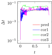
(a) Set 1 of tolerances

$\ell$	rtol	atol	error	naccept	nreject
0	1e–04	1e–06	2.031e–03	59	0
1	1e–06	1e–08	7.002e–05	81	61
2	1e–08	1e–10	1.412e–07	30	3
3	1e–10	1e–12	9.847e–08	60	33

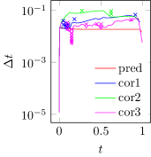
(b) Set 2 of tolerances

$\ell$	rtol	atol	error	naccept	nreject
0	1e–04	1e–06	2.031e–03	59	0
1	1e–05	1e–07	1.853e–04	31	10
2	1e–07	1e–09	1.505e–06	21	3
3	1e–09	1e–11	9.473e–07	44	14

Figure 10: Auzinger IVP: Different tolerances at each level. With the first set of tolerances, the step-size controller for the predictor is well behaved, as are the second and third correctors. The step-size controller for the first corrector however is noisy. With the second set of tolerances, the step-size controllers for all correctors are reasonably well behaved.

4.2.4 Using Solutions from the Error Equation

As mentioned in Subsection 3.3, using the solution from the error equation (5) as the local error estimate for step-size control on a given level is potentially problematic because the step-size controller can only control the local error introduced on that level whereas the true local error generally contains contributions from all previous levels. For completeness, we present the results of this adaptive RIDC formulation applied to the Auzinger problem (Figure 11) and the Orbit problem (Figure 12). Step-doubling is used for step-size adaptivity on the predictor level, solutions from the error equation are used to control step-sizes for the corrector levels. For the Auzinger problem, we observe in the top figure that if the tolerances are held fixed on each level, each correction level improves the solution. If the tolerance is reduced slightly on each level, the step-size controller gives a poor step-size selection (many rejected steps), even for this smoothly varying problem. For the Orbit IVP, Figure 12 shows that the corrector improves the solution if the tolerances are held fixed at all levels; however the corrector requires many steps. A second correction loop was not attempted. Reducing the tolerance for the first corrector resulted in inordinately many rejected steps.

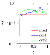
$\ell$	rtol	atol	error	naccept	nreject
0	1e–04	1e–06	2.031e–03	59	0
1	1e–04	1e–06	7.249e–04	33	3
2	1e–04	1e–06	6.513e–06	26	10

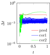
$\ell$	rtol	atol	error	naccept	nreject
0	1e–04	1e–06	2.031e–03	59	0
1	1e–05	1e–07	1.063e–05	657	305
2	1e–06	1e–08	9.446e–08	75	76

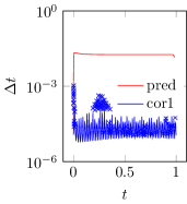
$\ell$	rtol	atol	error	naccept	nreject
0	1e–04	1e–06	2.031e–03	59	0
1	1e–07	1e–09	1.178e–07	60571	94

Figure 11: Auzinger Problem: Step-doubling on prediction levelz, using successive levels for error estimation for step control on the error equation. Step-size controller for the corrector is noisy.

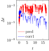
$\ell$	rtol	atol	error	naccept	nreject
0	1e–04	1e–04	2.405e–00	2261	230
1	1e–04	1e–04	7.234e–01	475181	84

Figure 12: Orbit Problem: Step-doubling on prediction level, using successive levels for error estimation for step control on the error equation.

5 Conclusions

In this paper, we formulated RIDC methods that incorporate local error estimation and adaptive step-size control. Several formulations were discussed in detail: (i) step-doubling on the prediction level, (ii) embedded RK pairs on the prediction level, (iii) step-doubling on the prediction and error levels, and (iv) step-doubling for the prediction level but using the solution from the error equation for step-size control; other formulations are also alluded to. A convergence theorem from [9] can be extended to RIDC methods that use adaptive step-size control on the prediction level. Numerical experiments demonstrate that RIDC methods with non-uniform steps converge as designed and illustrate the type of behavior that might be observed when adaptive step-size control is used on the prediction and correction levels. Based on our numerical study, we conclude that adaptive step-size control on the prediction level is viable for RIDC methods. In a practical application where a user gives a specified tolerance, this prescribed tolerance must be transformed to a specific tolerance that is fed to the predictor.

References

- [1] A. Christlieb, C. Macdonald, and B. Ong, “Parallel high-order integrators,” SIAM J. Sci. Comput., vol. 32, no. 2, pp. 818–835, 2010.
- [2] A. Christlieb and B. Ong, “Implicit parallel time integrators,” J. Sci. Comput., vol. 49, no. 2, pp. 167–179, 2011.
- [3] A. Christlieb, A. Melfi, and B. Ong, “Distributed parallel semi-implicit time integrators,” arXiv:1209.4297v1.
- [4] A. Christlieb, R. Haynes, and B. Ong, “A parallel space-time algorithm,” SIAM J. Sci. Comput., vol. 34, no. 5, pp. 233–248, 2012.
- [5] A. Dutt, L. Greengard, and V. Rokhlin, “Spectral deferred correction methods for ordinary differential equations,” BIT, vol. 40, no. 2, pp. 241–266, 2000.
- [6] E. Hairer, S. P. Nørsett, and G. Wanner, Solving ordinary differential equations. I, vol. 8 of Springer Series in Computational Mathematics. Berlin: Springer-Verlag, second ed., 1993. Nonstiff problems.
- [7] J. R. Dormand and P. J. Prince, “A family of embedded Runge-Kutta formulae,” J. Comput. Appl. Math., vol. 6, no. 1, pp. 19–26, 1980.
- [8] E. Hairer and G. Wanner, Solving ordinary differential equations. II, vol. 14 of Springer Series in Computational Mathematics. Berlin: Springer-Verlag, second ed., 1996. Stiff and differential-algebraic problems.
- [9] Y. Xia, Y. Xu, and C.-W. Shu, “Efficient time discretization for local discontinuous Galerkin methods,” Discrete Contin. Dyn. Syst. Ser. B, vol. 8, no. 3, pp. 677–693, 2007.
- [10] B. Bradie, A Friendly Introduction to Numerical Analysis: With C and MATLAB. Person Prentice Hall, 2006.
- [11] A. Christlieb, B. Ong, and J.-M. Qiu, “Comments on high order integrators embedded within integral deferred correction methods,” Comm. Appl. Math. Comput. Sci., vol. 4, no. 1, pp. 27–56, 2009.
- [12] A. Christlieb, B. Ong, and J.-M. Qiu, “Integral deferred correction methods constructed with high order Runge-Kutta integrators,” Math. Comput., vol. 79, pp. 761–783, 2010.
- [13] A. Christlieb, M. Morton, B. Ong, and J.-M. Qiu, “Semi-implicit integral deferred correction constructed with additive Runge–Kutta methods,” Commun. Math. Sci., vol. 9, no. 3, pp. 879–902, 2011.
- [14] W. Auzinger, H. Hofstätter, W. Kreuzer, and E. Weinmüller, “Modified defect correction algorithms for ODEs part I: General theory,” Numer. Algorithms, vol. 36, pp. 135–156, 2004.
- [15] S. Güttel and G. Klein, “Efficient high-order rational integration and deferred correction with equispaced data.” preprint.
- [16] P. Bogacki and L. F. Shampine, “A 3 (2) pair of runge-kutta formulas,” Applied Mathematics Letters, vol. 2, no. 4, pp. 321–325, 1989.
- [17] E. Fehlberg, “Low-order classical runge-kutta formulas with step size control and their application to some heat transfer problems,” tech. rep., NASA Techincal Report 315, 1969.