IFIC/13-77

Abstract:

Contrary to what is sometimes stated, the current electroweak precision data easily allow for massive composite resonance states at the natural EW scale, i.e., well over the TeV. The oblique parameters $S$ and $T$ are analyzed by means of an effective Lagrangian that implements the $SU(2)_{L}\otimes SU(2)_{R}\to SU(2)_{L+R}$ pattern of electroweak symmetry breaking. They are computed at the one-loop level and incorporating the newly discovered Higgs-like boson and possible spin–1 composite resonances. Imposing a proper ultraviolet behaviour is crucial and allows us to determine $S$ and $T$ at next-to-leading order in terms of a few resonance parameters. Electroweak precision data force the vector and axial-vector states to have masses above the TeV scale and suggest that the $W^{+}W^{-}$ and $ZZ$ couplings to the Higgs-like scalar should be close to the Standard Model value. Our findings are generic: they only rely on symmetry principles and soft requirements on the short-distance properties of the underlying strongly-coupled theory, which are widely satisfied in more specific scenarios.

1 Introduction

In this talk we present the first combined analysis of the oblique parameters $S$ and $T$ [1, 2], including the newly discovered Higgs-like boson and possible spin–1 composite resonances at the one-loop level [3, 4]. We consider a general Lagrangian implementing the $SU(2)_{L}\otimes SU(2)_{R}\to SU(2)_{L+R}$ pattern of electroweak symmetry breaking (EWSB), with a non-linear realization of the corresponding Goldstone bosons [5]. We consider strongly-coupled models where the gauge symmetry is dynamically broken by means of some non-perturbative interaction. Usually, theories of this kind do not contain a fundamental Higgs, bringing instead composite states of different types, in a similar way as it happens in Quantum Chromodynamics. In the past, electroweak (EW) chiral effective Lagrangians [5] were used for the study of the oblique parameters [6]. In the recent years, several works have incorporated vector and axial-vector resonances and performed one-loop computations of $S$ and $T$ within a similar $SU(2)_{L}\otimes SU(2)_{R}/SU(2)_{L+R}$ effective framework [7, 8]. However, they contained unphysical dependences on the ultraviolet (UV) cut-off, manifesting the need for local contributions to account for a proper UV completion. Our calculation avoids this problem through the implementation of short-distance conditions on the relevant Green functions, in order to satisfy the assumed UV behaviour of the strongly-coupled theory. As shown in Refs. [9, 10], the dispersive approach we adopt avoids all technicalities associated with the renormalization procedure, allowing for a much more transparent understanding of the underlying physics.

2 Electroweak effective theory

Let us consider a low-energy effective theory containing the Standard Model (SM) gauge bosons coupled to the EW Goldstones, one scalar state $S_{1}$ with mass $m_{S_{1}}=126$ GeV and the lightest vector and axial-vector resonance multiplets $V$ and $A$, which are expected to be the most relevant ones at low energies. We assume the SM pattern of EWSB and the scalar field $S_{1}$ is taken to be a singlet, whereas $V$ and $A$ are introduced as triplets.

The relevant one-loop absorptive diagrams we will compute require interaction vertices with at most three legs. In addition, since we just consider contributions from the lightest channels, $\varphi\varphi$ (two Goldstones) and $S_{1}\varphi$ for the $S$–parameter, and $\varphi B$ and $S_{1}B$ for $T$, we will just need the Lagrangian operators [3, 4]

$$\mathcal{L} = \bigg{(}\,1\,+\,\frac{\displaystyle 2\kappa_{W}}{\displaystyle v}\,S_{1}\,\bigg{)}\,\frac{\displaystyle v^{2}}{\displaystyle 4}\,\langle\,u_{\mu}u^{\mu}\,\rangle\,+\frac{F_{V}}{2\sqrt{2}}\,\langle\,V_{\mu\nu}f^{\mu\nu}_{+}\,\rangle+\frac{i\,G_{V}}{2\sqrt{2}}\,\langle\,V_{\mu\nu}[u^{\mu},u^{\nu}]\,\rangle$$ (1)

$$\qquad\qquad\qquad\qquad\qquad\qquad+\frac{F_{A}}{2\sqrt{2}}\,\langle\,A_{\mu\nu}f^{\mu\nu}_{-}\,\rangle+\sqrt{2}\,\lambda_{1}^{SA}\,\partial_{\mu}S_{1}\,\langle\,A^{\mu\nu}u_{\nu}\,\rangle\,,$$

with $u_{\mu}=\,-\vec{\sigma}\partial_{\mu}\vec{\varphi}/v+...$ and the other chiral tensors are defined in [4, 11]. In addition, we will have the Yang-Mills and gauge-fixing terms, with the computation performed in the Landau gauge. The term proportional to $\kappa_{W}$ in Eq. (1) contains the coupling of the scalar $S_{1}$ resonance to two gauge bosons. For $\kappa_{W}=1$ one recovers the $S_{1}\to\varphi\varphi$ vertex of the SM. The computation is performed in the Landau gauge.

3 Oblique parameters

The $S$–parameter measures the difference between the off-diagonal $W^{3}B$ correlator and its SM value, while $T$ parametrizes the breaking of custodial symmetry [1]:

$$S\,=\,\frac{\displaystyle 16\pi}{\displaystyle g^{2}}\;\big{(}e_{3}-e_{3}^{\rm SM}\big{)}\,,\qquad\qquad T\,=\,\frac{\displaystyle 4\pi}{\displaystyle g^{2}\sin^{2}{\theta_{W}}}\;\big{(}e_{1}-e_{1}^{\rm SM}\big{)}\,,$$ (2)

with

$$e_{3}\,=\,\frac{\displaystyle g}{\displaystyle g^{\prime}}\;\widetilde{\Pi}_{30}(0)\,,\qquad\qquad e_{1}\,=\,\frac{\displaystyle 1}{\displaystyle M_{W}^{2}}(\Pi_{33}(0)-\Pi_{WW}(0))\,.$$ (3)

The tree-level   Goldstone contribution  in $e_{3}$   has been removed from $\Pi_{30}(q^{2})$ in the form ${\Pi_{30}(q^{2})\,=\,q^{2}\,\widetilde{\Pi}_{30}(q^{2})+g^{2}\tan{\theta_{W}}\,v^{2}/4}$. For the computation of these oblique parameters we have made use of the dispersive representations [1, 3, 4]

$$S = \frac{\displaystyle 16\pi}{\displaystyle g^{2}\tan\theta_{W}}\;\displaystyle{\int}_{0}^{\infty}\frac{\displaystyle{\rm dt}}{\displaystyle t}\;[\rho_{S}(t)\,-\,\rho_{S}(t)^{\rm SM}]\,,$$ (4)

$$T = \frac{\displaystyle 4\pi}{\displaystyle g^{\prime\,2}\cos^{2}\theta_{W}}\;\displaystyle{\int}_{0}^{\infty}\frac{\displaystyle{\rm dt}}{\displaystyle t^{2}}\;[\rho_{T}(t)\,-\,\rho_{T}(t)^{\rm SM}]\,,$$ (5)

with the one-loop spectral functions (we will remain at lowest order in $g$ and $g^{\prime}$)

$$\rho_{S}(t) = \frac{\displaystyle 1}{\displaystyle\pi}\,\mbox{Im}\widetilde{\Pi}_{30}(t)\,,\qquad\qquad\rho_{T}(t)\,=\,\frac{1}{\pi}\mbox{Im}[\Sigma(t)^{(0)}-\Sigma(t)^{(+)}]\,.$$ (6)

The first dispersion relation (4) was worked out by Peskin and Takeuchi [1] and its convergence requires a vanishing spectral function at short distances. Since $\rho_{S}(t)^{\rm SM}$ vanishes at high energies, the spectral function $\rho_{S}(t)$ of the theory we want to analyze must also go to zero for $s\to\infty$. This removes from the picture any undesired UV cut-off and $S$ depends only on the physical scales of the problem. For the computation of $T$, we employ the Ward-Takahashi identity [12] which relates the $\Pi_{33}$ and $\Pi_{WW}$ polarizations with the EW Goldstone self-energies $\Sigma^{(0)}$ and $\Sigma^{(+)}$, respectively. In the Landau gauge one finds the next-to-leading order (NLO) relation ${e_{1}=\Sigma^{\prime}(0)^{(0)}\,-\,\Sigma^{\prime}(0)^{(+)}}$, with $\Sigma^{\prime}(t)\equiv\mathrm{\frac{d}{dt}}\Sigma(t)$ [3, 4]. We have computed the one-loop contributions to the Goldstone self-energies from the lightest two-particle absorptive cuts: $\varphi B$ and $S_{1}B$. Our analysis [3, 4] shows that, once proper short-distance conditions have been imposed on the form-factors that determine $\rho_{S}(t)$, the spectral function $\rho_{T}(t)$ also vanishes at high momentum and one is allowed to recover $T$ by means of the UV–converging dispersion relation (5). Nonetheless, we want to stress that this property, hinted previously by Ref. [8], has only been explicitly checked for the leading channels, $\varphi B$ and $S_{1}B$, contributing to $T$. The $1/t$ and $1/t^{2}$ weights in Eqs. (4) and (5), respectively, enhance the contribution from the lightest thresholds and suppress channels with heavy states [10]. Thus, in this talk we focus our attention on the lightest one and two-particle cuts: $\varphi$, $V$, $A$, $\varphi\varphi$ and $S_{1}\varphi$ for the $S$–parameter; $\varphi B$ and $S_{1}B$ for $T$. Since the leading-order (LO) determination of $S$ already implies that the vector and axial-vector masses must be above the TeV scale, two-particle cuts with $V$ and $A$ resonances are very suppressed. Their effect was estimated in Ref. [11] and found to be small.

4 Short-distance constraints: Weinberg sum-rules

Since we are assuming that weak isospin and parity are good symmetries of the strong dynamics, the correlator $\Pi_{30}(s)$ can be written in terms of the vector ($R+L$) and axial-vector ($R-L$) two-point functions as [1]

$$\Pi_{30}(s)\,=\,\frac{g^{2}\tan{\theta_{W}}}{4}\;s\;\left[\Pi_{VV}(s)-\Pi_{AA}(s)\right]\,.$$ (7)

In asymptotically-free gauge theories the difference $\Pi_{VV}(s)-\Pi_{AA}(s)$ vanishes at $s\to\infty$ as $1/s^{3}$ [13]. This implies two super-convergent sum rules, known as the 1st and 2nd Weinberg sum-rules (WSRs) [14]. At LO (tree-level), the 1st and 2nd WSRs imply, respectively, [1, 14]

$$F_{V}^{2}\,-\,F_{A}^{2}\,=\,v^{2}\,,\qquad\qquad F_{V}^{2}\,M_{V}^{2}\,-\,F_{A}^{2}\,M_{A}^{2}\,=\,0\,,$$ (8)

where the 1st (2nd) WSR stems from requiring $\Pi_{VV}(s)-\Pi_{AA}(s)$ to vanish faster than $1/s$ ($1/s^{2}$) at short distances. If both WSRs are valid, one has $M_{V}<M_{A}$ and the vector and axial-vector couplings $F_{V,A}$ can be determined at LO in terms of the resonance masses [1, 3, 4, 15]. On the other hand, if only the 1st WSR is assumed then the vector is no longer forced to be lighter than the axial-vector [16, 17]; all one can say is that $F_{V}^{2}>F_{A}^{2}$. It is likely that the 1st WSR is also true in gauge theories with non-trivial UV fixed points [8]. However, the 2nd WSR cannot be used in Conformal Technicolour models [8] and its validity is questionable in most Walking Technicolour scenarios [16].

The $\varphi\varphi$ and $S_{1}\varphi$ contributions to the spectral function $\rho_{S}(t)$ are given by

$$\rho_{S}(s)|_{\varphi\varphi} = \theta(s)\;\frac{\displaystyle g^{2}\tan\theta_{W}}{\displaystyle 192\pi^{2}}\;|\mathcal{F}^{v}_{\varphi\varphi}(s)|^{2}\,,$$ (9)

$$\rho_{S}(s)|_{S_{1}\varphi} = \mbox{}-\theta(s-m_{S_{1}}^{2})\;\frac{\displaystyle g^{2}\tan\theta_{W}}{\displaystyle 192\pi^{2}}\;|\mathcal{F}^{a}_{S_{1}\varphi}(s)|^{2}\;\left(1-\frac{\displaystyle m_{S_{1}}^{2}}{\displaystyle s}\right)^{3}\,,$$ (10)

with the $\varphi\varphi$ and $S_{1}\varphi$ form-factors, respectively, provided at LO by [3, 4, 10]

$$\mathcal{F}^{v}_{\varphi\varphi}(s) = 1\,+\,\sigma_{V}\;\frac{\displaystyle s}{\displaystyle M_{V}^{2}-s}\,,\qquad\qquad\mathcal{F}^{a}_{S_{1}\varphi}(s)=\kappa_{W}\;\left(\,1\,+\,\sigma_{A}\>\frac{\displaystyle s}{\displaystyle M_{A}^{2}-s}\,\right)\,,$$ (11)

with $\sigma_{V}\equiv F_{V}G_{V}/v^{2}$ and $\sigma_{A}\equiv F_{A}\lambda_{1}^{\mathrm{SA}}/(\kappa_{W}v)$. We will demand these form factors to fall as ${\cal O}(1/s)$, i.e., $\sigma_{V}=\sigma_{A}=1$ [3, 4]. When computing the $T$ parameter at NLO we found that the $\varphi B$ and $S_{1}B$ channels in the $\rho_{T}(t)$ spectral function were fully determined by the form-factors $\mathcal{F}^{v}_{\varphi\varphi}$ and $\mathcal{F}^{a}_{S_{1}\varphi}$, respectively [4]. This relation between the $\varphi\varphi$ vector form-factor and the $T$–parameter was also previously hinted in Ref. [8]. Thus, in addition to making $\Pi_{30}(t)$ and $\rho_{S}(t)$ well-behaved at short distances, these conditions alone lead to a good high-energy behaviour for the $\rho_{T}(t)$ spectral function [3, 4].

5 Theoretical predictions at LO and NLO

At leading order, the tree-level Goldstone self-energies are identically zero and one has ${T_{\rm LO}=0}$. On the other hand, for the $S$–parameter one obtains [1, 3, 4, 11]

$$S_{\rm LO} = \frac{\displaystyle 4\pi v^{2}}{\displaystyle M_{V}^{2}}\,\bigg{(}\,1\,+\,\frac{\displaystyle M_{V}^{2}}{\displaystyle M_{A}^{2}}\,\bigg{)}\,\qquad\qquad\mbox{(Two WSRs)}\,,$$ (12)

$$S_{\rm LO} > \frac{\displaystyle 4\pi v^{2}}{\displaystyle M_{V}^{2}}\qquad\qquad\qquad\qquad\mbox{(Only the 1st WSRs; $M_{V}<M_{A}$)}\,,$$ (13)

with the last inequality flipping sign (becoming an identity) in the inverted-mass scenario $M_{V}>M_{A}$ [16, 17] (degenerate-mass scenario $M_{V}=M_{A}$). Eq. (12) assumes the validity of the two WSRs, while only the 1st WSR is taken into account in Eq. (13), but assuming $M_{V}<M_{A}$. In both cases, the resonance masses need to be heavy enough to comply with the stringent experimental limits on $S$ [2], implying $M_{V}>1.5$ TeV (2.3 TeV) at the 3$\sigma$ (1$\sigma$) level.

At NLO, the requirement that Im$\widetilde{\Pi}_{30}(s)$ vanishes at short distances allows us to reconstruct the full correlator $\Pi_{30}(s)$ through a one subtracted dispersion relation [3, 4, 10, 11]:

$$\left.\Pi_{30}(s)\right|_{\mathrm{NLO}}\;=\;\frac{g^{2}\tan{\theta_{W}}}{4}\;s\;\left(\frac{v^{2}}{s}+\frac{F_{V}^{r\,2}}{M_{V}^{r\,2}-s}-\frac{F_{A}^{r\,2}}{M_{A}^{r\,2}-s}\;+\;\overline{\Pi}(s)\right)\,,$$ (14)

with the renormalized $F_{R}^{r}$ and $M_{R}^{r}$ and the finite one-loop contribution $\overline{\Pi}(s)$, fully determined by Im$\widetilde{\Pi}_{30}(s)$ (see App. A of Ref. [11]). By imposing the WSRs at NLO, one obtains NLO conditions on the high-energy expansion of $\Pi_{30}(s)|_{\rm NLO}$ in powers of $1/s$. Its real and imaginary parts allow us to constrain the renormalized resonance couplings $F_{V,A}^{r\,\,2}$ and produces the condition $\kappa_{W}=M_{V}^{2}/M_{A}^{2}$ (in the case with two WSRs), respectively. Thus, for the NLO $S$–parameter one finds [3, 4]

$$S = 4\pi v^{2}\left(\frac{1}{M_{V}^{2}}+\frac{1}{M_{A}^{2}}\right)\,+\,\frac{1}{12\pi}\,\left[\log\frac{M_{V}^{2}}{m_{H}^{2}}-\frac{11}{6}\right.\left.+\;\frac{M_{V}^{2}}{M_{A}^{2}}\log\frac{M_{A}^{2}}{M_{V}^{2}}-\frac{M_{V}^{4}}{M_{A}^{4}}\,\bigg{(}\log\frac{M_{A}^{2}}{m_{S_{1}}^{2}}-\frac{11}{6}\bigg{)}\right]$$ (15)

$$\quad\qquad\qquad\qquad\qquad\qquad\qquad\qquad\qquad\qquad\qquad\qquad\qquad\qquad\mbox{(Two WSRs)}\,,$$

$$S > \frac{\displaystyle 4\pi v^{2}}{\displaystyle M_{V}^{2}}\,\,+\,\,\frac{\displaystyle 1}{\displaystyle 12\pi}\left[\left(\ln\frac{\displaystyle M_{V}^{2}}{\displaystyle m_{H}^{2}}-\frac{\displaystyle 11}{\displaystyle 6}\right)-\,\kappa_{W}^{2}\,\left(\log\frac{\displaystyle M_{A}^{2}}{\displaystyle m_{S_{1}}^{2}}-\frac{\displaystyle 17}{\displaystyle 6}+\frac{\displaystyle M_{A}^{2}}{\displaystyle M_{V}^{2}}\right)\right]$$ (16)

$$\qquad\qquad\qquad\qquad\qquad\qquad\qquad\qquad\qquad\qquad\mbox{(Only the 1st WSR; $M_{V}<M_{A}$)}\,,$$

where $m_{H}$ sets the reference Higgs mass in the definition of the oblique parameters. We have used the renormalized masses in the NLO expressions and the superscript $r$ is dropped from now on. As in the LO case, in the case $M_{V}>M_{A}$ [16, 17] ($M_{A}=M_{V}$), the inequality (16) flips direction (becomes an identity).

As we saw in the previous section, one also has $\rho_{T}(t)\stackrel{{\scriptstyle t\to\infty}}{{\longrightarrow}}0$ for the $\varphi B$ and $S_{1}B$ channels once the $\rho_{S}(t)$ spectral function constraints $\sigma_{V}=\sigma_{A}=1$ are imposed and the form-factors vanish at high energies. The $T$ dispersion relation (5) becomes then UV convergent and yields [3, 4]

$$T\;=\;\frac{3}{16\pi\cos^{2}\theta_{W}}\;\left[1+\log{\frac{m_{H}^{2}}{M_{V}^{2}}}-\kappa_{W}^{2}\,\left(1+\log{\frac{m_{S_{1}}^{2}}{M_{A}^{2}}}\right)\right]\,.$$ (17)

Terms of $\mathcal{O}(m_{S_{1}}^{2}/M_{A}^{2})$ have been neglected in Eqs. (15)–(17). After imposing the high-energy constraints, the $S$ and $T$ determinations can be written in terms of two (three) parameters, e.g., $M_{V}$ and $\kappa_{W}$ ($M_{V}$, $M_{A}$ and $\kappa_{W}$), in the case with two WSRs (with only the 1st WSR).

6 Phenomenology

• 1) Case with two WSRs: In the more restrictive scenario, we find at 68% (95%) CL (Fig. 1):

  $$0.97\;(0.94)\;<\;\kappa_{W}\;<\;1\,,\qquad\qquad M_{A}\;>\;M_{V}\;>\;5\;(4)\>\mathrm{TeV}.$$ (18)

  As $\kappa_{W}=M_{V}^{2}/M_{A}^{2}$ due to the 2nd WSR at NLO, the vector and axial-vector turn out to be quite degenerate.

  

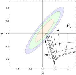
  Figure 1: NLO determinations of $S$ and $T$, imposing the two WSRs. The grid lines correspond to $M_{V}$ values from $1.5$ to $6.0$ TeV, at intervals of $0.5$ TeV, and $\kappa_{W}=0,0.25,0.50,0.75,1$. The arrows indicate the directions of growing $M_{V}$ and $\kappa_{W}$. The ellipses give the experimentally allowed regions at 68% (orange), 95% (green) and 99% (blue) CL [2].

• 2) Case with only the 1st WSR: The previous stringent bounds get softened when only the 1st WSR is required to be valid. On general grounds, one would expect this scenario to satisfy the mass hierarchy $M_{V}<M_{A}$. Assuming a moderate splitting $0.5<M_{V}/M_{A}<1$, we obtain (68% CL)

  $$0.84\;<\;\kappa_{W}\;<\;1.3\,,\qquad\qquad M_{V}\;>\;1.5\;\mathrm{TeV}.$$ (19)

  Slightly larger departures from the SM can be achieved by considering a larger mass splitting.
  When the resonance masses become degenerate, the allowed range for the scalar coupling shrinks to $0.97<\kappa_{W}<1.3$ (68% CL) (black band Fig. 2, right-hand side). A heavier resonance mass is also necessary, with $M_{V}=M_{A}>1.8$ TeV (68% CL).
  Finally, in the inverted-mass scenario, we obtain the upper bound $\kappa_{W}<2$ (68% CL) for $1<M_{V}/M_{A}<2$. Nonetheless, if no vector resonance is seen below the TeV ($M_{V}>1$ TeV) the scalar coupling becomes again constrained to be around $\kappa_{W}\simeq 1$ for $1<M_{V}/M_{A}<2$, with the 68% CL interval $0.7<\kappa_{W}<1.9$. The outcomes for various mass splittings in the different scenarios with only the 1st WSR (normal-ordered, degenerate and inverted-mass) can be observed in Fig. 2.

In summary, contrary to what is sometimes stated, the current electroweak precision data easily allow for resonance states at the natural EW scale, i.e., well over the TeV. The present results are in good agreement with the $H\to WW,ZZ$ couplings measured at LHC, compatible with the Standard Model up to deviations of the order of 20% or smaller [18]). These conclusions are generic, since we have only used mild assumptions about the UV behavior of the underlying strongly-coupled theory, and can be easily particularized to more specific models obeying the $SU(2)_{L}\otimes SU(2)_{R}\to SU(2)_{L+R}$ EWSB pattern.

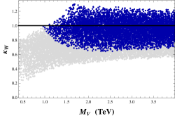
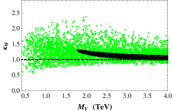
Figure 2: Left-hand side: Scatter plot for the 68% CL region, in the case when only the 1st WSR is assumed, for $M_{V}<M_{A}$. The dark blue and light gray regions correspond, respectively, to $0.2<M_{V}/M_{A}<1$ and $0.02<M_{V}/M_{A}<0.2$. Right-hand side: 68% CL region with only the 1st WSR for the degenerate and inverted-hierarchy scenarios. The black (dark) and green (lighter) regions correspond, respectively, to $M_{V}=M_{A}$ and $1<M_{V}/M_{A}<5$. We consider $M_{V,A}>0.4$ TeV in both plots.

References

- [1] M. E. Peskin and T. Takeuchi, Phys. Rev. D 46 (1992) 381; Phys. Rev. Lett. 65 (1990) 964.
- [2] M. Baak et al., Eur. Phys. J. C 72 (2012) 2205; http://gfitter.desy.de/ .
- [3] A. Pich, I. Rosell and J. J. Sanz-Cillero, Phys. Rev. Lett. 110 (2013) 181801; [arXiv:1307.1958 [hep-ph]].
- [4] A. Pich, I. Rosell and J.J. Sanz-Cillero, [arXiv:1310.3121 [hep-ph]].
- [5] T. Appelquist and C. W. Bernard, Phys. Rev. D 22 (1980) 200; A. C. Longhitano, Phys. Rev. D 22 (1980) 1166; Nucl. Phys. B 188 (1981) 118.
- [6] A. Dobado, D. Espriu and M. J. Herrero, Phys. Lett. B 255 (1991) 405.
- [7] S. Matsuzaki et al., Phys. Rev. D 75 (2007) 073002; 075012; R. Barbieri et al., Phys. Rev. D 78 (2008) 036012; O. Catà and J.F. Kamenik, Phys. Rev. D 83 (2011) 053010; A. Orgogozo and S. Rychkov, JHEP 1306 (2013) 014.
- [8] A. Orgogozo and S. Rychkov, JHEP 1203 (2012) 046;
- [9] A. Pich, I. Rosell and J.J. Sanz-Cillero, JHEP 0701 (2007) 039; JHEP 1102 (2011) 109.
- [10] A. Pich, I. Rosell and J. J. Sanz-Cillero, JHEP 0807 (2008) 014.
- [11] A. Pich, I. Rosell and J. J. Sanz-Cillero, JHEP 1208 (2012) 106.
- [12] R. Barbieri et al., Nucl. Phys. B 409 (1993) 105.
- [13] C. W. Bernard et al., Phys. Rev. D 12 (1975) 792.
- [14] S. Weinberg, Phys. Rev. Lett. 18 (1967) 507.
- [15] M. Knecht and E. de Rafael, Phys. Lett. B 424 (1998) 335.
- [16] T. Appelquist and F. Sannino, Phys. Rev. D 59 (1999) 067702.
- [17] D. Marzocca, M. Serone and J. Shu, JHEP 1208 (2012) 013 [arXiv:1205.0770 [hep-ph]].
- [18] ATLAS Collaboration, Phys. Lett. B 726 (2013) 88; ATLAS-CONF-2013-079 (July 19, 2013); CMS Collaboration, JHEP 06 (2013) 081; CMS-PAS-HIG-13-005 (April 17, 2013).