Comment on “Quantum versus classical instability of scalar fields in curved backgrounds” [arXiv:1310.2185]

Abstract

I show that the claim of the paper [arXiv:1310.2185] on the absence of instability for a minimally coupled scalar field on a static spherically symmetric gravitational background is incorrect.

The authors of the paper MMV claim that “… there are no tachyonic modes for minimally coupled scalar fields in asymptotically flat spherically symmetric static spacetimes containing no horizons…” (p. 2 and Appendix of MMV ). In fact, the authors tried to prove that there is no any Jeans instability in this case contrary to the results of psfss . This statement is, of course, incorrect as I shall show below.

Consider a static spherically symmetric metric [Eq. (1), MMV ]

$$ds^{2}=-e^{2\Xi(r)}dt^{2}+e^{2\Lambda(r)}dr^{2}+r^{2}(d\theta^{2}+\sin^{2}\theta d\phi^{2}).$$ (1)

Changing the variable [Eq. (14), MMV ]

$$x(r)=\int_{0}^{r}dr^{\prime}e^{\Lambda(r^{\prime})-\Xi(r^{\prime})},$$ (2)

the authors reduce this interval to

$$ds^{2}=e^{2\Xi}(-dt^{2}+dx^{2})+r^{2}d\Omega^{2}.$$ (3)

Then, the variables in the massless KG equation,

$$(\nabla^{2}-\xi R)\Phi=0,$$ (4)

are separated,

$$\Phi=e^{-i\omega t}\frac{\psi_{\omega l}(r)}{r}Y_{lm}(\theta,\phi),$$ (5)

and the radial part of the KG equation becomes

$$-\psi^{\prime\prime}+\Big{[}\frac{r^{\prime\prime}}{r}+e^{2\Xi}\big{(}\frac{l(l+1)}{r^{2}}+\xi R\big{)}\Big{]}\psi=\omega^{2}\psi,$$ (6)

where all the derivatives are taken with respect to $x$. For the $s$-wave ($l=0$) and for the minimal coupling, $\xi=0$, it becomes

$$-\psi^{\prime\prime}+\frac{r^{\prime\prime}}{r}\psi=\omega^{2}\psi,$$ (7)

As follows from Eq. (14), the function $r(x)$ is an arbitrary smooth function on the interval $x\in[0,+\infty)$, but obeying the restrictions

1. $r^{\prime}(x)>0$,  $x\in[0,+\infty)$,

2. $\lim_{x\rightarrow+\infty}r^{\prime}(x)=1$.

In Appendix of MMV , the authors provide an obscure reasoning that Eq. (7) has no bound states for any $r(x)$ satisfying the requirements above. If the latter took place then the general statement proposed by the authors (see the first paragraph) would hold.

However, it is clear from (7) that one can simply draw the monotonic function $r(x)$ satisfying all the requirements and possessing a negative second derivative on a sufficiently large interval such that the effective potential,

$$V_{eff}=r^{\prime\prime}/r,$$ (8)

admits bound states. To be more specific, I shall give the explicit example.

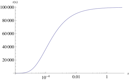
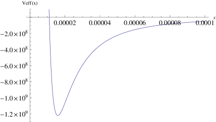
Figure 1: Left panel: The plot of $r(x)$ with $a=10^{-2}$, $b=10^{5}$, and $\alpha=1/2$. Right panel: The plot of $V_{eff}(x)=r^{\prime\prime}/r$ with $a=10^{-2}$, $b=10^{5}$, and $\alpha=1/2$.

Consider the function

$$r(x)=x+be^{-a/x^{\alpha}},\quad a,b,\alpha>0.$$ (9)

It complies with all the requirements above. I take $a=10^{-2}$, $b=10^{5}$, and $\alpha=1/2$. The plots of $r(x)$ and $V_{eff}$ with these parameters are given in Fig. 1. The profile of the effective potential resembles the Lennard-Jones one. In order to prove that $V_{eff}$ possesses the bound states, I use the quasiclassical criterion (the Borh-Sommerfeld quantization rule)

$$\int_{x_{1}}^{x_{2}}dx\sqrt{-r^{\prime\prime}/r}\geq\pi/2,$$ (10)

where $x_{1}$ and $x_{2}$ are the turning points. If the turning point $x_{1}=0$ then the RHS of this inequality should be replaced by $\pi/4$. In our case, one can find that $x_{1}\approx 1.11\times 10^{-5}$, $x_{2}=+\infty$, and the numerical evaluation of the integral (10) results in

$$\int_{x_{1}}^{+\infty}dx\sqrt{-r^{\prime\prime}/r}\approx 4.7>\pi/2.$$ (11)

Thus the bound state exists. Curiously enough, this example can be treated analytically at very large $b$. In this case, in evaluating the integral (10), one may replace

$$r(x)\approx be^{-a/x^{\alpha}}\;\Rightarrow\;V_{eff}=\frac{\alpha^{2}a^{2}}{x^{2\alpha+2}}-\frac{\alpha(\alpha+1)a}{x^{\alpha+2}},\qquad x_{1}=\Big{(}\frac{\alpha a}{\alpha+1}\Big{)}^{1/\alpha}.$$ (12)

The LHS of (10) equals $\pi(1+\alpha^{-1})/2$ and can be made as large as one wants by choosing sufficiently small $\alpha$. In particular, in the case $\alpha=1/2$ we have $3\pi/2\approx 4.7$. Of course, one may object that the example above is somewhat unphysical. Nevertheless it provides a counterexample to the general statement of MMV .

Moreover, one can prove that the instability (tachyonic modes) exists even in a more physically reasonable situation. Using the fact that

$$r^{\prime\prime}/r=e^{2(\Xi-\Lambda)}\frac{\Xi^{\prime}_{r}-\Lambda^{\prime}_{r}}{r}=r^{\prime 2}\frac{\Xi^{\prime}_{r}-\Lambda^{\prime}_{r}}{r},$$ (13)

the integral (10) can be rewritten as

$$\int_{x_{1}}^{x_{2}}dx\sqrt{-r^{\prime\prime}/r-e^{2\Xi}\xi R}=\int_{r_{1}}^{r_{2}}dr\sqrt{(\Lambda^{\prime}_{r}-\Xi^{\prime}_{r})/r-e^{2\Lambda}\xi R},$$ (14)

where the nonminial coupling has been restored. Then, employing the Einstein equations for a static spherically symmetric metric LandLifshCTF , we have

$$\int_{x_{1}}^{x_{2}}dx\sqrt{-r^{\prime\prime}/r-e^{2\Xi}\xi R}=\int_{r_{1}}^{r_{2}}dr\Big{[}-4\pi Ge^{2\Lambda}(T^{t}_{t}+T^{r}_{r}-2\xi T)+(1-e^{2\Lambda})/r^{2}\Big{]}^{1/2}\geq\pi/2.$$ (15)

At large $r$, one can neglect the terms at $r^{-2}$ and obtain

$$\int_{r_{1}}^{r_{2}}dre^{\Lambda}\Big{[}-4\pi G(T^{t}_{t}+T^{r}_{r}-2\xi T)\Big{]}^{1/2}\geq\pi/2.$$ (16)

Introducing the Jeans length (see, e.g., GorbRub ),

$$\lambda_{J}:=\Big{(}\frac{\pi c_{s}^{2}}{G\varepsilon}\Big{)}^{1/2},$$ (17)

where $\varepsilon$ is the energy density and $c_{s}$ is the sound speed in the matter, which I assume to be a fluid with

$$p=c_{s}^{2}\varepsilon,$$ (18)

one can estimate from (16) the characteristic wavelengths $\ell$ of unstable modes. Roughly,

$$\ell\geq\frac{\lambda_{J}}{4c_{s}\sqrt{1-2\xi-(1-6\xi)c_{s}^{2}}},$$ (19)

in the weak field limit. The case $\xi=1/6$ corresponds to the conformal coupling. If the radicand in (19) is nonpositive then one may expect that there is no such an instability. However, we see that for an ultrarelativistic fluid, $c_{s}^{2}=1/3$, this instability takes place for any $\xi$. It also always exist at $\xi\in[0,1/2]$ and, in particular, for the minimal and conformal couplings. Thus the Bose-Einstein condensation discussed in psfss exist even in the weak field limit for the minimal coupling contrary to the claims of MMV . Such a condensation develops on the scales comparable with the structure formation scale of the Universe.

References

• (1) R. F. P. Mendes, G. E. A. Matsa, and D. A. T. Vanzella, Quantum versus classical instability of scalar fields in curved backgrounds, arXiv:1310.2185.
• (2) P. O. Kazinski, Propagator of a scalar field on a stationary slowly varying gravitational background, arXiv:1211.3448; P. O. Kazinski, I. S. Kalinichenko, High-temperature expansion of the one-loop free energy of a scalar field on a curved background, Phys. Rev. D. 87, 084036 (2013), arXiv:1301.5103.
• (3) L. D. Landau, E. M. Lifshitz, The Classical Theory of Fields (Butterworth-Heinemann, San Francisco, 1994), Sec. 100.
• (4) D. S. Gorbunov, V. A. Rubakov, Introduction to the Theory of Early Universe Vol. 1 (Krasand, Moscow, 2009) [in Russian], Sec. 1.1.