The Planetary System to KIC 11442793: A Compact Analogue to the Solar System

Abstract

We announce the discovery of a planetary system with 7 transiting planets around a Kepler target, a current record for transiting systems. Planets b, c, e and f are reported for the first time in this work. Planets d, g and h were previously reported in the literature (Batalha et al., 2013), although here we revise their orbital parameters and validate their planetary nature. Planets h and g are gas giants and show strong dynamical interactions. The orbit of planet g is perturbed in such way that its orbital period changes by 25.7h between two consecutive transits during the length of the observations, which is the largest such perturbation found so far. The rest of the planets also show mutual interactions: planets d, e and f are super-Earths close to a mean motion resonance chain (2:3:4), and planets b and c, with sizes below 2 Earth radii, are within 0.5% of the 4:5 mean motion resonance. This complex system presents some similarities to our Solar System, with small planets in inner orbits and gas giants in outer orbits. It is, however, more compact. The outer planet has an orbital distance around 1 AU, and the relative position of the gas giants is opposite to that of Jupiter and Saturn, which is closer to the expected result of planet formation theories. The dynamical interactions between planets are also much richer.

1 Introduction

Finding planetary systems similar to our own is one of the main goals of exoplanet search. It is of particular interest if such systems show planetary transits, since multiple transiting planetary systems provide crucial information for the understanding of planet formation and evolution (Ford & Gaudi, 2006). Mutual dynamical interactions between planets especially require an additional effort to understand their origin and to justify their long term stability. Unfortunately, such systems are difficult to find because of the low geometrical probability for transiting planets. The satellite Kepler (Borucki et al., 2010) has observed the planetary system orbiting the star KIC 11442793 almost continuously for more than 4 years. The Kepler team has published the parameters of 3 transiting candidates around this star (Batalha et al., 2013) with the identification numbers KOI 351.01, .02, and .03. A careful analysis of the light curve with the transit detection algorithm DST (Cabrera et al., 2012) reveals the presence of 4 additional transiting planets, making this system the most populated among the transiting ones. These 4 planets are reported here for the first time (see the results of Ofir & Dreizler 2013; Huang et al. 2013; Tenenbaum et al. 2013). Considering the magnitude of the star (13.7 magnitude in SDSS r) and the characteristics of the transiting candidates, we were not able to independently confirm the planets by measuring their masses with radial velocity. However, we have performed the following steps to validate the planetary nature of the candidates: 1) medium resolution spectra of the star were taken with the Coudé-Echelle spectrograph at the Tautenburg observatory, characterizing the host star as a solar-like dwarf; 2) the analysis of the Kepler photometry, including the study of the motion of the PSF centroid (Batalha et al., 2010), which does not reveal any hint of the presence of contaminating eclipsing binary; 3) the analysis of the timing of the eclipses reveals that the planetary candidates are dynamically interacting one with each other; and finally 4) a stability analysis of the system with the orbital dynamics integrator Mercury (Chambers, 1999) reveals that, for the system to be stable, all the planetary candidates must have planetary masses. Therefore, we validate in this paper the planetary nature of the 7 candidates.

2 Stellar characterization

In order to characterize the host star, five spectra were taken on June 6 and 7, 2013, with the Coudé-Echelle spectrograph attached to the 2-m telescope at the Thüringer Landessternwarte Tautenburg. The wavelength coverage was 472-736 nm and a 2 arcsec slit provided a spectral resolving power of $32\,000$. The exposure time for each spectrum was 40 minutes.

The spectra were reduced using standard ESO-MIDAS packages. The reduction steps included filtering of cosmic rays, background and straylight subtraction, flat fielding using a halogen lamp, optimum extraction of diffraction orders, and wavelength calibration using a ThAr lamp. Due to the low signal-to-noise ratio (SNR) of a single spectrum it was difficult to define the local continuum. Because no radial velocity shifts between the single spectra could be found, we repeated the reduction using the co-added raw spectra. The continuum of the resulting mean spectrum was then well enough defined for a proper normalization. The SNR of the mean spectrum, measured from some almost line-free parts of the continuum, was about 19.

We used the spectral synthesis method, which compared the observed spectrum with synthetic spectra computed on a grid in atmospheric parameters. The synthetic spectra were computed with the SynthV program (Tsymbal, 1996), based on a library of atmosphere models calculated with the LLmodels code (Shulyak et al., 2004). The error estimation was done from $\chi^{2}$ statistics taking all interdependencies between the different parameters into account (Lehmann et al., 2011).

The step widths of the grid were 100K in T_eff, 0.1 dex in $\log g$, 0.1 dex in [M/H], 0.5 km s^-1 in microturbulent velocity, and 1 km s^-1 in $v\sin i$; where [M/H] means scaled solar abundances. For the determination of $v\sin i$ we used the metal lines-rich wavelengths region 491-567 nm. For all other parameters, the wavelengths range utilized was 472-567 nm which also includes H_β.

Table 1 lists the results obtained from the full grid in all parameters. The large uncertainties mainly originate from the large ambiguities between the different parameters and from the low SNR of the observed spectrum. We use a compilation of empirical values of stellar parameters from (Gray, 2005). Comparing our results from the full grid search with the literature data, we see that we can exclude luminosity class III stars because of the values of $\log g$ and v$\sin i$. The $T_{\mathrm{eff}}$ derived from spectral analysis lies, within the uncertainties, between $5\,600$ and $6\,250$K which is consistent with dwarfs of spectral type G6 to F6. Based on the measured $\log g$, we cannot determine if the star is slightly evolved. Assuming that the star is a typical main sequence star of early G-type, we can adopt a $\log g$ of 4.4, which lies within the measurement error, obtaining a better constraint on on $T_{\mathrm{eff}}$ and a slightly higher value for the metallicity (last column of Table 1). Under this assumption, we obtain $T_{\mathrm{eff}}$ between $5\,910$ and $6\,340$ K, corresponding to spectral types between G1 and F6. The corresponding ranges in mass and radius are relatively small, between 1.1 and 1.3 M_sun and 1.1 and 1.3 R_sun.

2.1 Reddening and distance

We determined the interstellar extinction $A_{\mathrm{v}}$ and distance $d$ to KIC 11442793 by applying the method described in Gandolfi et al. (2008). This technique is based on the simultaneous fit of the observed stellar colours with theoretical magnitudes obtained from the NextGen model spectrum (Hauschildt et al., 1999) with the same photospheric parameters as the target star. For KIC 11442793 we used SDSS, 2MASS, and WISE photometry (see Table 2 and Fig. 1). We excluded the $W_{3}$ and $W_{4}$ WISE magnitudes, as the former has a SNR of 3.5 and the latter is only an upper limit. Assuming a normal extinction ($R_{\mathrm{v}}=3.1$) and a black body emission at the stellar effective temperature and radius, we found that the star reddening amounts to $A_{\mathrm{v}}=0.15\pm 0.10$ mag and that the distance to KIC 11442793 is $d=780\pm 100$ pc.

Figure 1: Dereddened spectral energy distribution of KIC 11442793. The optical SDSS-$g$,-$r$,-$i$,-$z$ photometry is from the Kepler Input Catalogue. Infrared $J$,$H$,$Ks$ and $W1$, $W2$, $W3$, $W4$ data are taken from the 2MASS (Cutri et al., 2003) and WISE (Wright et al., 2010) database, respectively. The NextGen model spectrum by Hauschildt et al. (1999) with the same photospheric parameters as KIC 11442793 and scaled to the stellar radius and distance is overplotted with a light-blue line.

Table 1: Derived atmospheric parameters for the star.

	full grid	$\log g$ fixed
Teff (K)	$5\,930\pm 320$	$6\,080^{+260}_{-170}$
$\log g$ (cgs)	$4.0\pm 0.5$	$4.4$ (fixed)
vmic (km s-1)	$1.2\pm 0.6$	$1.2\pm 0.6$
$[$M/H$]$ (dex)	$-0.17\pm 0.21$	$-0.12\pm 0.18$
v $\sin i$ (km s-1)	$4.6\pm 2.1$	$4.6\pm 2.1$

Table 2: Kepler, GSC2.3, USNO-A2, and 2MASS identifiers of the target star. Equatorial coordinates and optical SDSS-$g$,-$r$,-$i$,-$z$ photometry are from the Kepler Input Catalogue. Infrared $J$,$H$,$Ks$ and $W1$,$W2$,$W3$,$W4$ data are taken from the 2MASS (Cutri et al., 2003) and WISE (Wright et al., 2010) database, respectively.

Main identifiers
Kepler IDs	KIC 11442793 - KOI 351 - Kepler-90
GSC2.3 ID	N2EM001018
USNO-A2 ID	1350-10067455
2MASS ID	18574403+4918185
Equatorial coordinates
RA  (J2000) $18^{h}\,57^{m}\,44^{s}.038$	Dec (J2000) $+49^{\mathrm{o}}18^{\prime}18^{\prime\prime}.58$
Magnitudes
Filter   ($\lambda_{\mathrm{e}ff}$)	Mag	Uncertainty
$g$     ( 0.48 $\mu m$)	14.139	0.030
$r$     ( 0.63 $\mu m$)	13.741	0.030
$i$     ( 0.77 $\mu m$)	13.660	0.030
$z$     ( 0.91 $\mu m$)	13.634	0.030
$J$     ( 1.24 $\mu m$)	12.790	0.029
$H$    ( 1.66 $\mu m$)	12.531	0.033
$Ks$  ( 2.16 $\mu m$)	12.482	0.024
$W_{1}$  ( 3.35 $\mu m$)	12.429	0.024
$W_{2}$  ( 4.60 $\mu m$)	12.462	0.024
$W_{3}$  (11.56 $\mu m$)	12.750	0.308
$W_{4}$  (22.09 $\mu m$)	$~{}~{}9.702^{a}$	-

^aUpper limit

3 Light curve analysis

Kepler observations of KIC 11442793 extend for $1\,340$ days with a duty cycle of 82%. The light curve, shown in Figure 2, reveals that the host star is not particularly active. It barely shows hints of some variations compatible with the evolution of stellar spots on its surface, with an amplitude of 0.1%

We have applied a detrending algorithm to treat the stellar activity optimized for the CoRoT mission (Baglin et al., 2006), but adapted to the treatment of Kepler data (Cabrera et al., 2012). Then we have applied the transit detection algorithm DST (Cabrera et al., 2012) to search for the periodic signature of transiting planets.

We confirm the detection of the candidates KOI 351.01, .02, and .03, previously announced (Batalha et al., 2013), and we assign them the identifications KIC 11442793 h, g, and d. We present the discovery of four additional candidates, b, c, e, and f, reported for the first time here. The ephemerides of these objects are given in Table 3. The orbital ephemerides have been calculated as follows: the transit detection algorithm DST provides preliminary values of the period, epoch, depth and duration of the transiting candidates. With this information, we first fit separately the transits of every candidate. Then we make a weighted linear fit to the epochs of the individual transits, the slope of the fit is the period and the intercept the epoch.The residuals between the linear fit and the actual position of the transits (observed minus calculated, O-C) are usually referred as transit timing variations (TTVs), which are discussed later on Section 5.

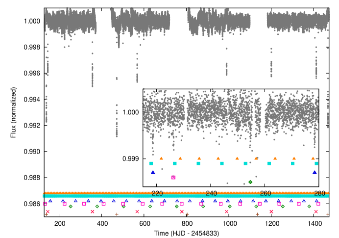
Figure 2: Public raw light curve of KIC 11442793. The seven sets of periodic transits are indicated with symbols of different colors: planet h with red plus-signs, planet g with red crosses, planet f with green diamonds, planet e with magenta squares, planet d with blue triangles, planet c with turquoise filled squares, and planet b with orange filled triangles. In the enlarged region the stellar variability has been subtracted to show a subset of the shallower transits.

4 Planetary parameter modelling

Several planets in this system show significant transit timing variations (TTVs), described in Section 5, which need to be removed before proceeding with the modeling of the planetary parameters. We use an iterative method to correct for this effect, similar to the one described by Alapini & Aigrain (2009), but accounting for the TTVs. We take a geometrical model of the transit based on the preliminary value of the planetary parameters obtained by the detection method. We use a genetic algorithm (Geem et al., 2001) to fit the value of the epoch, fixing the other transit parameters. For every trial value of the epoch, we correct for stellar activity in a region covering ten times the transit duration with a second order Legendre polynomial (first order for planets b and c). The polynomial is interpolated in the expected region of the transit, to preserve the transit shape. We then fold the light curve with the obtained values of the individual epochs. This method does not converge in the case of planets b and c because of the low SNR of their transit signal. Therefore, for planets b and c we fix the period, we do not fit for the epochs, but we do apply the stellar activity correction for each individual transit described above.

A detailed description of the modeling of the planetary parameters applied here can be found in Csizmadia et al. (2011). We used the publicly available short cadence Kepler light curves. For candidates b, c, d, e and f we binned the light curves (we formed 2000 binned points in the $\pm 2D$ vicinity of the mid-transit, $D$ being the transit duration), while for candidates g and h we used the original short cadence photometric points. We used the Mandel & Agol (2002) transit model. This model gives the light loss of the star due to the transit of an object as a function of their size ratio (k), of their mutual sky-projected distance (denoted by $\delta$), and of the limb darkening coefficients of the transited star ($ld_{1}=u_{1}+u_{2},$ and $ld_{2}=u_{1}-u_{2}$).

Following Csizmadia et al. (2013) we determined the limb darkening coefficients from the light curve instead of using theoretical predictions. This fit was first applied to planet h, which has the largest transit depth i.e. the highest signal-to-noise ratio. Having obtained the values of the limb darkening coefficients, we set the limb darkening coefficients at the value obtained from the fit of planet g’s transit light curve, but we allowed them to vary within the uncertainties of the determined values.

Since we do not have any radial velocity measurements, nor occultations, nor phase-curves of any of these seven planets, we had no a priori information about eccentricities and arguments of periastron. Therefore we could not calculate the sky-projected distance of the stellar and planetary centers in the usual way (e.g. Giménez 2006). Instead, we fitted the duration of the transit, the epoch ($t_{0}$), the period ($P$), the impact parameter ($b$), the planet-to-stellar radii ratio ($k=R_{p}/R_{s}$). Then the sky-projected mutual distance of the star and the planet were calculated with the formula

$$\delta\approxeq\sqrt{b^{2}+\left[(1+k)^{2}-b^{2}\right]\left(\frac{t-t_{0}}{P}\right)^{2}}$$ (1)

where $t$ is the time. We checked the validity of this latter formula via numerical experiments and we found that in our cases it yields a very good agreement with the theoretical value in the vicinities of transits. No mutual transit event was modeled. For the optimization, a genetic algorithm process described in Csizmadia et al. (2011) was used, and the results were refined by a Simulated Annealing algorithm which was also used for the error estimation. The reported uncertainties in Table 3 are 1$\sigma$ uncertainties.

We report the modeled values of $k$ and $b$ in Table 3 with their respective uncertainties for each of the seven candidates in the system. Once $k$, $b$, $D$, $P$ became known from the modeling procedure, the value of the scaled semi-major ($a/R_{s}$) for circular orbits can then be calculated as

$$\frac{a}{R_{s}}=\frac{1}{\pi}\frac{P}{D}\sqrt{(1+k)^{2}-b^{2}}$$ (2)

We then calculated the scaled semi-major axes for every planet in the system assuming circular orbits (see Table 3). Re-writing Kepler’s third law, we obtained for the stellar density parameter (neglecting the mass of the planet):

$$\frac{M^{1/3}}{R_{s}}=\left(\frac{3\pi}{GP^{2}}\right)^{1/3}\frac{a}{R_{S}}$$ (3)

or equivallentily

$$\frac{M^{1/3}}{R_{s}}=\left(\frac{3}{GPD}\right)^{1/3}\left[(1+k)^{2}-b^{2}\right]^{(3/2)}\left(\frac{1-e^{2}}{1+e^{2}-2e\sin\omega}\right)^{3/2}$$ (4)

We also report the density parameter derived from every candidate in Table 3. Figure 3 shows in graphical form the modelling of the photometric light curves and the model residuals for each planet.

Table 3: Planetary parameters. Values calculated for $R_{s}=1.2\pm 0.1R_{\odot}$; $R_{\odot}=696\,342$km and $R_{E}=6\,378$ km.

KIC 11442793 h (KOI 351.01)		KIC 11442793 d (KOI 351.03)
period (days)	331.600 59 $\pm$ 0.000 37	period (days)	59.736 67 $\pm$ 0.000 38
epoch (HJD - 2454833)	140.496 31 $\pm$ 0.000 82	epoch (HJD - 2454833)	158.965 6 $\pm$ 0.004 2
duration (h)	14.737 $\pm$ 0.046	duration (h)	8.40 $\pm$ 0.19
$a/R_{s}$	180.7 $\pm$ 4.7	$a/R_{s}$	56.1 $\pm$ 4.8
$a$ (AU)	1.01 $\pm$ 0.11	$a$ (AU)	0.32 $\pm$ 0.05
$R_{p}/R_{s}$	0.0866 $\pm$ 0.0007	$R_{p}/R_{s}$	0.0219 $\pm$ 0.0005
$R_{p}$ ($R_{E}$)	11.3 $\pm$ 1.0	$R_{p}$ ($R_{E}$)	2.87 $\pm$ 0.30
$b$	0.36 $\pm$ 0.07	$b$	0.28 $\pm$ 0.25
$i$ (deg)	89.6 $\pm$ 1.3	$i$ (deg)	89.71 $\pm$ 0.29
$M^{1/3}/R_{s}$	0.90 $\pm$ 0.13	$M^{1/3}/R_{s}$	0.88 $\pm$ 0.15
$ld_{1}$	0.348 $\pm$ 0.056	$ld_{1}$	0.371 $\pm$ 0.087
$ld_{2}$	1.03 $\pm$ 0.19	$ld_{2}$	1.04 $\pm$ 0.23
KIC 11442793 g (KOI 351.02)		KIC 11442793 c
period (days)	210.606 97 $\pm$ 0.000 43	period (days)	8.719 375 $\pm$ 0.000 027
epoch (HJD - 2454833)	147.036 4 $\pm$ 0.001 4	epoch (HJD - 2454833)	139.568 7 $\pm$ 0.002 3
duration (h)	12.593 $\pm$ 0.045	duration (h)	4.41 $\pm$ 0.18
$a/R_{s}$	127.3 $\pm$ 4.1	$a/R_{s}$	16.0 $\pm$ 0.8
$a$ (AU)	0.71 $\pm$ 0.08	$a$ (AU)	0.089 $\pm$ 0.012
$R_{p}/R_{s}$	0.0615 $\pm$ 0.0011	$R_{p}/R_{s}$	0.0091 $\pm$ 0.0003
$R_{p}$ ($R_{E}$)	8.1 $\pm$ 0.8	$R_{p}$ ($R_{E}$)	1.19 $\pm$ 0.14
$b$	0.45 $\pm$ 0.10	$b$	0.09 $\pm$ 0.20
$i$ (deg)	89.80 $\pm$ 0.06	$i$ (deg)	89.68 $\pm$ 0.74
$M^{1/3}/R_{s}$	0.84 $\pm$ 0.14	$M^{1/3}/R_{s}$	0.90 $\pm$ 0.16
$ld_{1}$	0.34 $\pm$ 0.10	$ld_{1}$	0.40 $\pm$ 0.20
$ld_{2}$	0.98 $\pm$ 0.10	$ld_{2}$	1.21 $\pm$ 0.26
KIC 11442793 f		KIC 11442793 b
period (days)	124.914 4 $\pm$ 0.001 9	period (days)	7.008 151 $\pm$ 0.000 019
epoch (HJD - 2454833)	254.704 $\pm$ 0.014	epoch (HJD - 2454833)	137.690 6 $\pm$ 0.001 7
duration (h)	10.94 $\pm$ 0.25	duration (h)	3.99 $\pm$ 0.15
$a/R_{s}$	86.4 $\pm$ 9.7	$a/R_{s}$	13.2 $\pm$ 1.8
$a$ (AU)	0.48 $\pm$ 0.09	$a$ (AU)	0.074 $\pm$ 0.016
$R_{p}/R_{s}$	0.0220 $\pm$ 0.0022	$R_{p}/R_{s}$	0.0100 $\pm$ 0.0005
$R_{p}$ ($R_{E}$)	2.88 $\pm$ 0.52	$R_{p}$ ($R_{E}$)	1.31 $\pm$ 0.17
$b$	0.35 $\pm$ 0.40	$b$	0.13 $\pm$ 0.32
$i$ (deg)	89.77 $\pm$ 0.31	$i$ (deg)	89.4 $\pm$ 1.5
$M^{1/3}/R_{s}$	0.84 $\pm$ 0.20	$M^{1/3}/R_{s}$	0.85 $\pm$ 0.21
$ld_{1}$	0.360 $\pm$ 0.068	$ld_{1}$	0.378 $\pm$ 0.060
$ld_{2}$	1.01 $\pm$ 0.18	$ld_{2}$	1.11 $\pm$ 0.20
KIC 11442793 e
period (days)	91.939 13 $\pm$ 0.000 73
epoch (HJD - 2454833)	134.312 7 $\pm$ 0.006 3
duration (h)	9.71 $\pm$ 0.19
$a/R_{s}$	74.7 $\pm$ 4.3
$a$ (AU)	0.42 $\pm$ 0.06
$R_{p}/R_{s}$	0.0203 $\pm$ 0.0005
$R_{p}$ ($R_{E}$)	2.66 $\pm$ 0.29
$b$	0.27 $\pm$ 0.22
$i$ (deg)	89.79 $\pm$ 0.19
$M^{1/3}/R_{s}$	0.87 $\pm$ 0.15
$ld_{1}$	0.360 $\pm$ 0.049
$ld_{2}$	1.05 $\pm$ 0.17

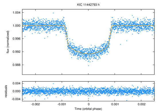
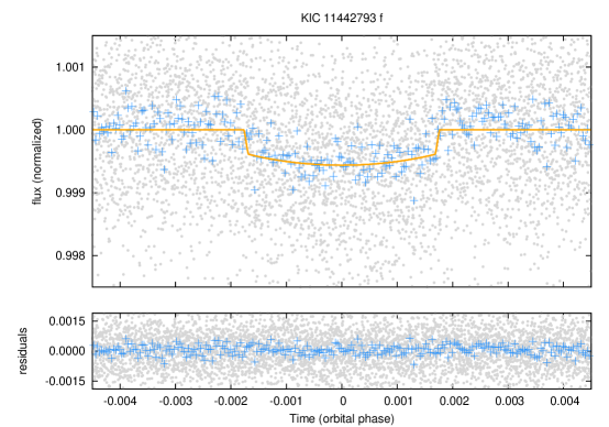
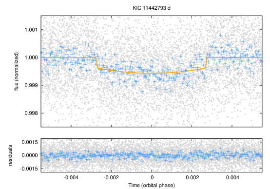
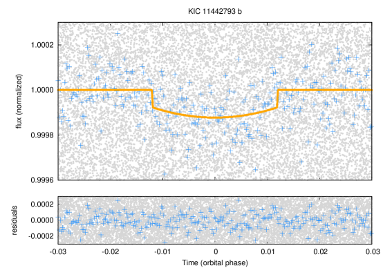
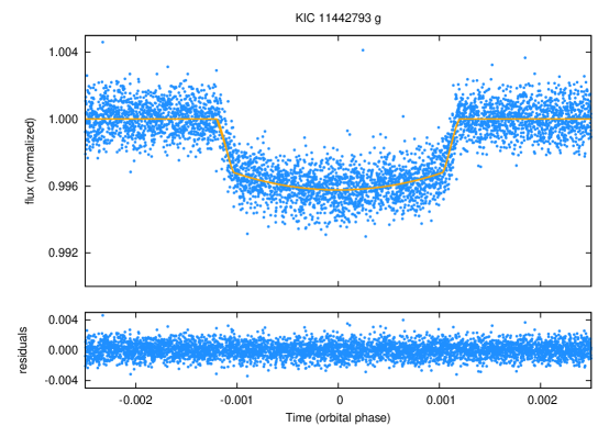
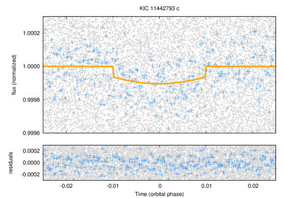
Figure 3: Filtered light curve of KIC 11442793 folded at the period of the different planets. For planets b and c the light curve has been binned, to help the eye. The orange solid line shows the light curve fit (Table 3). The lower panels show respectively the residuals of the light curve fit.

4.1 Analysis of the geometry of the transits

One argument supporting the hypothesis that all these planet candidates orbit the same star comes from the modeling of the planetary parameters. The inclinations and stellar densities ($M^{1/3}/R_{s}$) shown in Table 3 were calculated independently for each planet. They are all compatible to each other and the density is compatible with the value obtained independently for the stellar parameters in Section 2.

We can also provide another geometrical argument supporting the former hypothesis using the measured durations and periods of the transiting planets. These are obtained from a pure geometrical fit to the transits, independently of the planetary modelling techniques. This argument has previously been used in the literature to support the hypothesis that multiple candidate systems actually orbit the same star (Chaplin et al., 2013). Figure 4 shows how the transit durations distribute as a function of planetary periods. If all planets orbit the same star in circular, coplanar orbits, the transit duration $D$ should relate to the orbital period $P$ through Kepler’s third law:

$$D=\frac{\alpha}{\pi}P^{1/3}\sqrt{1-\left(\frac{\cos i}{\alpha}^{2}P^{4/3}\right)},$$ (5)

where $\alpha=(3\pi/G/\rho_{s})^{1/3}$, and $\rho_{s}$ is the density of the star. If $D$ and $P$ are in days, the best fit to the data gives a value of $\alpha=0.23$ and $i=90^{\circ}$, compatible with the values obtained from the stellar and planetary modelling. Note that the fit is not a physical solution, because all planetary orbits do not need to be exactly coplanar. However, they are compatible with all planets orbiting the same star in nearly edge-on aligned orbits, which supports our hypothesis that all planets orbiting the same star.

Figure 4: Transit duration of each planet as a function of their orbital period. The observed values are compatible with the seven planets orbiting a star whose density is that given by the stellar and planetary parameter modelling on edge-on aligned orbits. The range allowed by the modelling of the stellar parameters is indicated with the continuous blue lines.

5 Transit timing variations

The analysis of the transit timing variations (TTVs) has proved to be a versatile tool to confirm the planetary nature of transiting candidates (Ford et al., 2011). Typically, TTVs have amplitudes of several minutes (with some exceptional cases like KOI 142, Nesvorný et al. 2013, with an amplitude of 12h) and typically periods one order of magnitude larger than the orbital period of the planet involved (Mazeh et al., 2013).

Figure 5 shows the individual transits and Fig. 6 the O-C diagram for candidate g. The transit corresponding to epoch 7 (epoch 1 being the value provided in Table 3) has a displacement of 25.7 hours with respect to its expected position. This abrupt change is due to a change in the osculating orbital elements produced by the gravitational interaction with other objects in the system, possibly candidate h (see Section 6). Most surveys of TTVs expect discovering periodic modulations of the timing perturbations (see a derivation of the searched expression in Lithwick et al. 2012 and the series of papers  Ford et al. 2011, 2012a; Steffen et al. 2012a; Fabrycky et al. 2012; Ford et al. 2012b; Steffen et al. 2012b, 2013; Mazeh et al. 2013). However, non-periodic, sudden changes of the orbital elements, corresponding to irregular behavior such as the one displayed by planet g, have been theoretically described (for example, though in a different context, Holman & Murray 2005), but we believe that we report an observational example for the first time.

In addition to the change in the osculating elements, it is interesting to discuss separately the other transit events recorded for candidate g. The depth and the duration of transit events 1, 2, and 3 changes significantly. One can speculate that the perturbations seen around these transits are morphologically equivalent to those produced by a moon around the planet (Sartoretti & Schneider, 1999; Kipping et al., 2013b). This hypothesis is further discussed in Section 7.1. We do not have enough evidence to prove that these perturbations are produced by a moon and until we have constraints on the planetary masses we cannot assess the stability of moons around candidate g. We note, just for completion, that a moon could not be responsible in any case for the abrupt change in the osculating orbital elements displayed in transit event 7. The amplitudes of the perturbations produced by moons are typically only a few seconds (Cabrera, 2010; Kipping, 2009a, b).

The available data set for KIC 11442793 does not allow us to do an unambiguous determination of the planetary masses from the analysis of the TTVs. Candidates b and c are too small and too close to the detection limit to measure any reliable TTV amplitude (see Figure 6), which is not unusual in the case of low-mass planets in compact systems (see the case of CoRoT-7b Léger et al. 2009). The TTVs of candidates d and e are compatible with zero within the limits of our current modelling (see Figure 6). There are only 5 full transits observed from the 9 expected transits of candidate f due to some unfortunate coincidence of observing interruptions with the expected transit positions. However, there is a significant signal in the available O-C diagram, which means that candidate f is interacting dynamically with other objects in the system.

Candidate g shows 6 transits in the available data set (expected 7) and candidate h shows 3 transits (expected 5), less than expected due to the interruptions of the photometric record (duty cycle is 82%). However, candidates g and h show both significant TTVs and also transit duration variations, consequently we deduce that they are interacting dynamically.

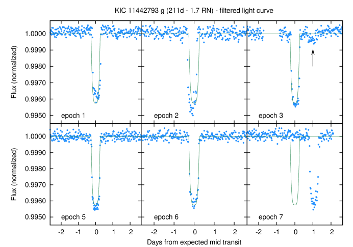
Figure 5: Individual observed transit events of planet g and the expected position of those transits assuming a constant period, marked with a line. Note the irregularities in the transit depth and duration at epochs 1 and 2 and the displacement from the expected position of epoch 7. The additional transit like event marked with an arrow close to epoch 3 is discussed in the text.

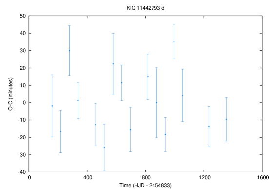
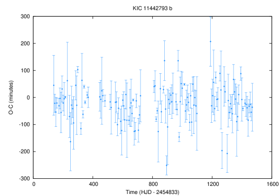
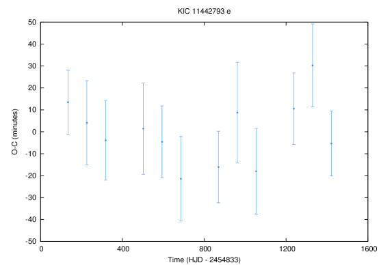
Figure 6: Transit timing variations of the different planets. Observed mid-times of planetary transits (O) minus calculated linear ephemeris (C) are plotted with 1$\sigma$ uncertainties.

6 Dynamical study

6.1 Analysis with a numerical integrator

We have done a stability analysis of the system with the orbital dynamics integrator Mercury (Chambers, 1999). The system is only stable if candidates g and h have masses below some Jupiter units (typically, less than 5 Jupiter masses). Therefore, we conclude that g and h are planets because they interact gravitationally and their long term dynamical stability is only guaranteed if these bodies have planetary masses.

The Mercury numerical analysis of the planetary system reveals that objects d, e, and f are in stable orbits only if those are very circular (typically, less than 3% for mass values of 10 Earth masses, representative of 2.5 Earth radii super-Earths) and planetary masses (less than the mass of Jupiter). Therefore, we conclude that these three must also be planets. Actually, the requirement of the circularity of their orbits implies that, for the system to be stable, the mean motion resonance has to play a role to guarantee the survival of the system.

We did not see any sign that candidates b and c interact dynamically with the other planets in the system because the low SNR of the transit light curves. The Mercury numerical analysis reveals that their orbits are in principle only stable if the objects have planetary masses.

6.2 A first dynamical study

We estimated the masses of the seven planets considering their sizes and assuming representative mean densities for each planetary class (gas giant, ice giants, large and small super-Earth) as follows: planet $m_{h}=0.8M_{\textrm{Jupiter}}$, $m_{g}=0.7M_{\textrm{Neptune}}$, planets $m_{f}\sim m_{e}\sim m_{d}\sim 10M_{\textrm{Earth}}$ and planets $m_{c}\sim m_{b}\sim 3M_{\textrm{Earth}}$. Given the the periods and the estimated semi-major axes we can compute their separation in terms of Hill radii. Using the formula given below (Chambers et al., 1996):

$$H=\left(\frac{m_{1}+m_{2}}{3}\right)^{\frac{1}{3}}\frac{a_{1}+a_{2}}{2}$$ (6)

we get the following numbers for the separation of neighboring planets in Hill radii:

$$g-h:5,h-f:11,f-e:5,e-d:10,d-c:47,\;\mathrm{and}\;c-b:10.$$ (7)

This indicates the stability of the different subsystem given they are moving in almost circular orbits. Especially the inner planets b, c, d, e and f are relative safe in their orbits, which is evident from their Hill radii. It is interesting to note, that the innermost two planets are in a 4:5 mean motion resonance (MMR); the two massive outer ones are not far from a 5:8 MMR. It is also worth to mention that the three planets d, e and f are close to the interesting Laplace resonance, which is known to happen for the the motion of the three Galilean Moons of Jupiter (Io, Europa and Ganymede) but also for the three Moons of Uranus (Miranda, Ariel and Umbriel, e.g. Ferraz-Mello 1979):

$$\frac{1}{P_{d}}-\frac{3}{P_{e}}+\frac{2}{P_{f}}\sim 0$$ (8)

Because the inner system consisting of super-earth planets is quite stable we concentrate on the dynamics of the planets h and g. The stability of this extrasolar planetary system seems to depend on the stability of the orbits of these two outer gas giants, which may have even eccentric orbits given the relative distance to the star. So we tried to find borders for stable motion of the two outer gas giants using the results of long term integrations up to $10^{7}$ years.

It turned out that inside the domain of motion for $e_{h}<0.095$ and $e_{g}<0.025$ the orbits of the two outer planets are regular with only slight periodic changes in the eccentricities (see Fig. 8, lower right graph). The closeness to the 8:5 MMR is not destroying their stability; an additional resonance appears for the motions of the perihelia of g and h. This secular resonance is depicted in Fig.7, where the 1:1 resonance of the motion of $\omega_{g}$ and $\omega_{h}$ with a period of about $1.7\cdot 10^{4}$ years is visible.

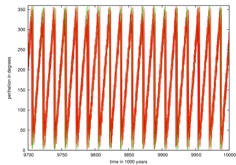
Figure 7: Perihelion motion of the two outer planets h and g for initial conditions in the stable domain (see text). Out of the whole integration time of $10^{7}$ years we show the first $3\cdot 10^{5}$ (upper graph) and the last $3\cdot 10^{5}$ years (lower graph). The strong coupling in a 1:1 secular resonance of the perihelion motion with a period of around $17\cdot 10^{4}$ is clearly visible.

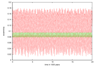
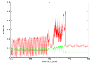
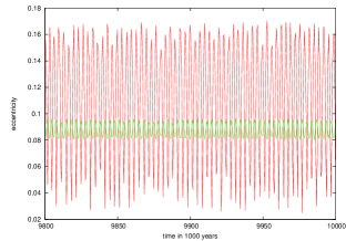
Figure 8: Orbits close to the stability region: time evolution of the eccentricities of the orbits of planets h (green) and g (red). Stable seeming orbit (upper left) which turns out to be unstable after about $7.69\cdot 10^{5}$ years (upper right). Another close by orbit unstable after $5.\cdot 10^{6}$ years (lower left); another close by, but stable orbit is shown (lower right). For details, see text.

Close to the edge of the stable region we have an intermediate region where stable and unstable orbits are very close to each other (see Fig. 8). In this domain we find the so-called sticky orbits - a well known phenomenon of dynamical systems (e.g. Dvorak et al. 1998): an orbit there is ’sticked’ to an invariant torus in phase space and then escapes through a hole of the last KAM-torus. We show in the respective figure three such examples, where a small shift in eccentricity of planet h ($\Delta e=0.005$) causes such a different dynamical behavior of an orbit.

We need to explain the large TTV for planet g: the answer is visible from Fig.9, where one can see the relatively large variations of the semi-major axis of this planet even for a time scale of years. This change can lead to a change in the period which achieves values up to a day from one transit to another one, comparable to the changes observed in the Kepler data.

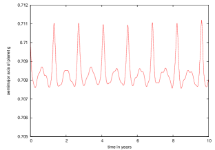
Figure 9: Variation of the semi-major axis of planet g caused by the presence of planet h during 10 years (left graph). Variation of the semi-major axis of the outer gas giant caused by the inner gas giant g (red color) and vice versa on planet g (green color) during $10^{3}$ years (right graph). Note that the lower curve is normalized with respect to the semi-major axis of a=0.71 AU of planet g

But the system is quite more complex: because planet g is in 5:3 MMR with planet f and this one is in the formerly mentioned Laplace resonance (with the planets e and d) the stability limit for the eccentricities of all planets is very small. Integrating the ’complete’ system it is only stable well before the stability limit mentioned above for the eccentricities of planets h and g: this absolute limit for a stable system is $e<0.001$ for all 5 outer planets!

We conclude from the preliminary dynamical study of this seven planet system that with the actual parameters determined it is quite close to instability. Consequently the parameters like the masses and the semi-major axes need some revision after a deeper dynamical study, out of the scope of this paper. Even in our Solar System, where the orbital parameters are well determined, the issue of the long term stability is debated (e.g. Laskar 1994, 2008) and the influence of many different resonances is complex. We are currently working on that dynamical study (Dvorak et al. in preparation).

7 KIC 11442793 in the context of other multiplanet systems

Models of planet formation include theories about planet-planet scattering followed by tidal circularization (Rasio & Ford, 1996; Lin & Ida, 1997; Chatterjee et al., 2008; Beaugé & Nesvorný, 2012). Another possible mechanism of planet formation builds planets at relative large distances of the star and later these planets migrate inwards through a disk (Goldreich & Tremaine, 1980; Lin et al., 1996; Ward, 1997; Murray et al., 1998). The first mechanism does not likely form compact multiple systems such the ones observed by Kepler (Batalha et al., 2013), characterized by being compact and by having low relative inclination orbits (Fang & Margot, 2012; Tremaine & Dong, 2012). Different mechanisms have been proposed to explain the origin of the latter systems. One promising possibility is in-situ formation, see for example (Chiang & Laughlin, 2013; Chatterjee & Tan, 2013), including the observed feature that many of those systems have planets orbiting close to, but not exactly at, mean motion resonances (Lithwick & Wu, 2012; Petrovich et al., 2013).

We show in Fig. 10 a schematic view of the periods and relative sizes of 9 multiple transiting planetary systems discovered by Kepler with 5 transiting planets or more, together with the planetary system reported in this paper. There are also multiple systems discovered by radial velocity hosting 6 or more planets, like GJ 667C (Anglada-Escudé et al., 2013), HD 40307 (Tuomi et al., 2013), or HD 10180 (Lovis et al., 2011). But their orbital properties and even their existence is not as secure as those of transiting candidates. For example, consider the case of the system GJ 581 (Hatzes, 2013) or the discussion in the literature if HD 10180 is orbited by six (Feroz et al., 2011), seven (Lovis et al., 2011), or even nine (Tuomi, 2012) planets. Therefore, we limit ourselves in Fig. 10 to the discussion of multiple transiting systems. Among the systems shown, KIC 11442973 presented here is the only one showing a clear hierarchy, like our Solar System. Additionally, only KIC 11442973 and KOI 435 include a giant planet larger than 10 Earth radii. Such systems are typically more difficult to form because giant planets tend to excite the eccentricity of less massive planets during the migration processes, compromising the long term stability of the system (see, for example, Raymond et al. 2008). Note that there are two additional known systems hosting simultaneously super-Earths and gas giants, but these two systems orbit M dwarfs, and only the second example is a compact system. GJ 676A (Anglada-Escudé & Tuomi, 2012) hosts up to 4 planets, including one super-Earth in a 3.6 days orbit and one 5 Jupiter masses planet in a 1050 days orbit. GJ 876 (Rivera et al., 2010) is also an M-dwarf hosting one super-Earth of 6 Earth masses at 1.9 days orbital period, a 0.7 Jupiter masses planet at 20 days, a 2.3 Jupiter masses planet at 61 days, and a 14 Earth masses planet in a 124 days orbit. However, KIC 11442793 is a late F/early G solar-like star, hosting a more complex system where dynamical interactions play an important role in the long term stability of the system.

7.1 About the possible existence of moons in the planetary system

We have discussed in previous sections the possibility that KIC 11442793g hosts a moon. Figure 5 shows that the transit epochs 1, 2 and 3 show features morphologically equivalent to an exomoon orbiting the planet (Sartoretti & Schneider, 1999; Szabó et al., 2006; Kipping, 2011). However, considering the distance between the transit epoch 3 and the moon-like event marked with an arrow in Figure 5, the estimated projected distance between the planet and the exomoon candidate would be orbiting close to the Hill radius of the planet, which is too far away to guarantee the long term stability of the satellite, usually limited to a distance of one third (Barnes & O’Brien, 2002) to one half (Domingos et al., 2006) of the planetary Hill sphere. With the current data set, we cannot exclude that the event marked with an arrow in Figure 5 is caused by instrumental residuals. However, the distorted shape features of transits 1 and 2 cannot be explained simply by the impact of stellar activity and their origin remains unclear. Space surveys have regularly been used to rule out the presence of moons around extrasolar planets (Pont et al., 2007; Deeg et al., 2010). So far, the most extensive search for exomoons (Kipping et al., 2012) has taken the advantage of the simultaneous change in the transit timing and transit duration changes produced by the hypothetical satellites (Kipping, 2009a, b). However, until now only negative results have been reported (Kipping et al., 2013b, a). A possible reason for this lack of success is that searches have been limited to isolated, typically non-giant planets. However, if these systems are formed by planet-planet scattering, they are unlikely to maintain the moons during their formation process (Gong et al., 2013). In turn, migration tends to remove moons from planetary systems (Namouni, 2010). Therefore, in-situ formed compact systems could be more prone to host exomoons in long timescales.

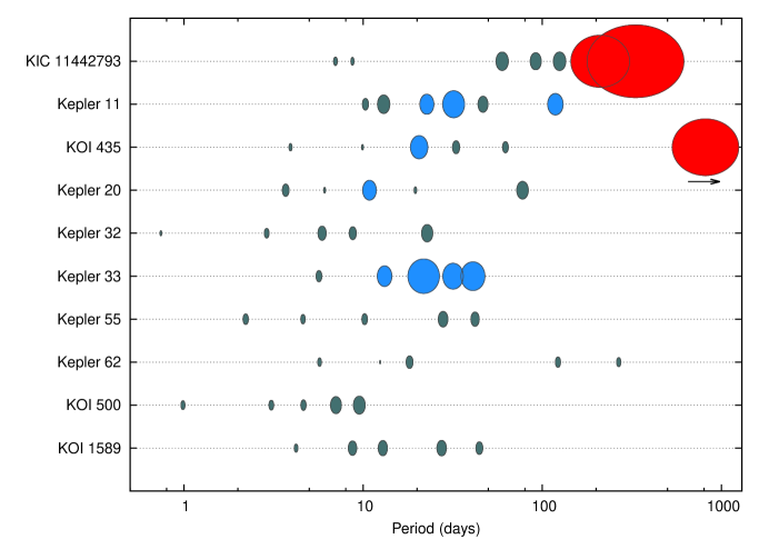
Figure 10: Comparison of different multiple systems. Kepler-11 (Lissauer et al., 2011), KOI-435 (Ofir & Dreizler, 2013), Kepler-20 (Gautier et al., 2012; Fressin et al., 2012), Kepler-32 (Fabrycky et al., 2012), Kepler-33 (Lissauer et al., 2012), Kepler-55 (Steffen et al., 2013), Kepler-62 (Borucki et al., 2013), KOI-500 (Xie, 2013; Wu & Lithwick, 2013), KOI-1589 (Xie, 2013; Wu & Lithwick, 2013). Color codes separate Earth and Super-Earth planets (up to 4 Earth radii, shown in green), Neptune-sized planets (between 4 and 8 Earth radii, shown in blue), and gas giants (larger than 8 Earth radii, shown in red).

8 Summary

We report the discovery of a planetary system with seven transiting planets with orbital periods in the range from 7 to 330 days (0.074 to 1.01 AU). The system is hierarchical, the two innermost planets have sizes close to Earth and their period ratio is within 0.5% of the 4:5 mean motion resonance. The three following planets are super-Earths with sizes between 2 and 3 Earth radii whose periods are close to a 2:3:4 chain. From the observational data set we cannot determine their masses or the value of their mean longitudes, but the ratio of their mean motions is close to a Laplace resonance. The outermost planets are two gas giants at distances of 0.7 and 1.0 AU. There are other systems of super-Earths, discovered either by radial velocity or by transit,which show some similarities, for example GJ 876 (Rivera et al., 2010) or KOI 152 (Wang et al., 2012), but these systems only contain super-Earths, while KIC 11442793 is a hierarchical system. As a singularity among the other multiple systems found by Kepler or radial velocity, KIC 11442793 contains a gas giant planet similar to Jupiter orbiting at 1 AU. Systems with super-Earths close to a Laplace resonance are also believed to be frequent (Chiang & Laughlin, 2013), but this particular system poses new challenges due to the presence of the gas giants g and h, which seem to have the most intense gravitational interaction measured among extrasolar planets so far (25.7 h of change in the ephemeris). If Kepler cannot continue the follow up of this system (Cowen, 2013), the follow-up of the Earth and super-Earth planets of this system will be challenging in the near future, as they are beyond reach for CHEOPS (Broeg et al., 2013) or TESS (Ricker et al., 2010). Only PLATO (Rauer & Catala, 2011) will be able to study in detail their evolution. However, the gas giants g and f produce 0.5% and 0.8% transits, which should be observable from ground, which makes of this system an attractive target for future follow-up studies.

References

- Alapini & Aigrain (2009) Alapini, A., & Aigrain, S. 2009, MNRAS, 397, 1591
- Anglada-Escudé & Tuomi (2012) Anglada-Escudé, G., & Tuomi, M. 2012, A&A, 548, A58
- Anglada-Escudé et al. (2013) Anglada-Escudé, G., Tuomi, M., Gerlach, E., et al. 2013, A&A, 556, A126
- Baglin et al. (2006) Baglin, A., Auvergne, M., Boisnard, L., et al. 2006, in COSPAR, Plenary Meeting, Vol. 36, 36th COSPAR Scientific Assembly, 3749
- Barnes & O’Brien (2002) Barnes, J. W., & O’Brien, D. P. 2002, ApJ, 575, 1087
- Batalha et al. (2010) Batalha, N. M., Rowe, J. F., Gilliland, R. L., et al. 2010, ApJ, 713, L103
- Batalha et al. (2013) Batalha, N. M., Rowe, J. F., Bryson, S. T., et al. 2013, ApJS, 204, 24
- Beaugé & Nesvorný (2012) Beaugé, C., & Nesvorný, D. 2012, ApJ, 751, 119
- Borucki et al. (2010) Borucki, W. J., Koch, D., Basri, G., et al. 2010, Science, 327, 977
- Borucki et al. (2013) Borucki, W. J., Agol, E., Fressin, F., et al. 2013, Science, 340, 587
- Broeg et al. (2013) Broeg, C., Fortier, A., Ehrenreich, D., et al. 2013, in European Physical Journal Web of Conferences, Vol. 47, European Physical Journal Web of Conferences, 3005
- Cabrera (2010) Cabrera, J. 2010, in EAS Publications Series, Vol. 42, EAS Publications Series, ed. K. Gożdziewski, A. Niedzielski, & J. Schneider, 109–116
- Cabrera et al. (2012) Cabrera, J., Csizmadia, S., Erikson, A., Rauer, H., & Kirste, S. 2012, A&A, 548, A44
- Chambers (1999) Chambers, J. E. 1999, MNRAS, 304, 793
- Chambers et al. (1996) Chambers, J. E., Wetherill, G. W., & Boss, A. P. 1996, Icarus, 119, 261
- Chaplin et al. (2013) Chaplin, W. J., Sanchis-Ojeda, R., Campante, T. L., et al. 2013, ApJ, 766, 101
- Chatterjee et al. (2008) Chatterjee, S., Ford, E. B., Matsumura, S., & Rasio, F. A. 2008, ApJ, 686, 580
- Chatterjee & Tan (2013) Chatterjee, S., & Tan, J. C. 2013, ArXiv e-prints, arXiv:1306.0576
- Chiang & Laughlin (2013) Chiang, E., & Laughlin, G. 2013, MNRAS, 431, 3444
- Cowen (2013) Cowen, R. 2013, Nature, 497, 417
- Csizmadia et al. (2013) Csizmadia, S., Pasternacki, T., Dreyer, C., et al. 2013, A&A, 549, A9
- Csizmadia et al. (2011) Csizmadia, S., Moutou, C., Deleuil, M., et al. 2011, A&A, 531, A41
- Cutri et al. (2003) Cutri, R. M., Skrutskie, M. F., van Dyk, S., et al. 2003, 2MASS All Sky Catalog of point sources.
- Deeg et al. (2010) Deeg, H. J., Moutou, C., Erikson, A., et al. 2010, Nature, 464, 384
- Domingos et al. (2006) Domingos, R. C., Winter, O. C., & Yokoyama, T. 2006, MNRAS, 373, 1227
- Dvorak et al. (1998) Dvorak, R., Contopoulos, G., Efthymiopoulos, C., & Voglis, N. 1998, Planet. Space Sci., 46, 1567
- Fabrycky et al. (2012) Fabrycky, D. C., Ford, E. B., Steffen, J. H., et al. 2012, ApJ, 750, 114
- Fang & Margot (2012) Fang, J., & Margot, J.-L. 2012, ApJ, 761, 92
- Feroz et al. (2011) Feroz, F., Balan, S. T., & Hobson, M. P. 2011, MNRAS, 415, 3462
- Ferraz-Mello (1979) Ferraz-Mello, S. 1979, Dynamics of the Galilean satellites - an introductory treatise
- Ford & Gaudi (2006) Ford, E. B., & Gaudi, B. S. 2006, ApJ, 652, L137
- Ford et al. (2011) Ford, E. B., Rowe, J. F., Fabrycky, D. C., et al. 2011, ApJS, 197, 2
- Ford et al. (2012a) Ford, E. B., Fabrycky, D. C., Steffen, J. H., et al. 2012a, ApJ, 750, 113
- Ford et al. (2012b) Ford, E. B., Ragozzine, D., Rowe, J. F., et al. 2012b, ApJ, 756, 185
- Fressin et al. (2012) Fressin, F., Torres, G., Rowe, J. F., et al. 2012, Nature, 482, 195
- Gandolfi et al. (2008) Gandolfi, D., Alcalá, J. M., Leccia, S., et al. 2008, ApJ, 687, 1303
- Gautier et al. (2012) Gautier, III, T. N., Charbonneau, D., Rowe, J. F., et al. 2012, ApJ, 749, 15
- Geem et al. (2001) Geem, Z. G., Kim, J. H., & Loganathan, G. V. 2001, Simulation, 76, 60, http://sim.sagepub.com/cgi/content/abstract/76/2/60
- Giménez (2006) Giménez, A. 2006, A&A, 450, 1231
- Goldreich & Tremaine (1980) Goldreich, P., & Tremaine, S. 1980, ApJ, 241, 425
- Gong et al. (2013) Gong, Y.-X., Zhou, J.-L., Xie, J.-W., & Wu, X.-M. 2013, ApJ, 769, L14
- Gray (2005) Gray, D. F. 2005, The Observation and Analysis of Stellar Photospheres
- Hanslmeier & Dvorak (1984) Hanslmeier, A., & Dvorak, R. 1984, A&A, 132, 203
- Hatzes (2013) Hatzes, A. P. 2013, Astronomische Nachrichten, 334, 616
- Hauschildt et al. (1999) Hauschildt, P. H., Allard, F., & Baron, E. 1999, ApJ, 512, 377
- Holman & Murray (2005) Holman, M. J., & Murray, N. W. 2005, Science, 307, 1288
- Huang et al. (2013) Huang, X., Bakos, G. Á., & Hartman, J. D. 2013, MNRAS, 429, 2001
- Kipping (2009a) Kipping, D. M. 2009a, MNRAS, 392, 181
- Kipping (2009b) —. 2009b, MNRAS, 396, 1797
- Kipping (2011) —. 2011, MNRAS, 416, 689
- Kipping et al. (2012) Kipping, D. M., Bakos, G. Á., Buchhave, L., Nesvorný, D., & Schmitt, A. 2012, ApJ, 750, 115
- Kipping et al. (2013a) Kipping, D. M., Forgan, D., Hartman, J., et al. 2013a, ArXiv e-prints, arXiv:1306.1530
- Kipping et al. (2013b) Kipping, D. M., Hartman, J., Buchhave, L. A., et al. 2013b, ApJ, 770, 101
- Laskar (1994) Laskar, J. 1994, A&A, 287, L9
- Laskar (2008) —. 2008, Icarus, 196, 1
- Léger et al. (2009) Léger, A., Rouan, D., Schneider, J., et al. 2009, A&A, 506, 287
- Lehmann et al. (2011) Lehmann, H., Tkachenko, A., Semaan, T., et al. 2011, A&A, 526, A124
- Lin et al. (1996) Lin, D. N. C., Bodenheimer, P., & Richardson, D. C. 1996, Nature, 380, 606
- Lin & Ida (1997) Lin, D. N. C., & Ida, S. 1997, ApJ, 477, 781
- Lissauer et al. (2011) Lissauer, J. J., Fabrycky, D. C., Ford, E. B., et al. 2011, Nature, 470, 53
- Lissauer et al. (2012) Lissauer, J. J., Marcy, G. W., Rowe, J. F., et al. 2012, ApJ, 750, 112
- Lithwick & Wu (2012) Lithwick, Y., & Wu, Y. 2012, ApJ, 756, L11
- Lithwick et al. (2012) Lithwick, Y., Xie, J., & Wu, Y. 2012, ApJ, 761, 122
- Lovis et al. (2011) Lovis, C., Ségransan, D., Mayor, M., et al. 2011, A&A, 528, A112
- Mandel & Agol (2002) Mandel, K., & Agol, E. 2002, ApJ, 580, L171
- Mazeh et al. (2013) Mazeh, T., Nachmani, G., Holczer, T., et al. 2013, ApJS, 208, 16
- Murray et al. (1998) Murray, N., Hansen, B., Holman, M., & Tremaine, S. 1998, Science, 279, 69
- Namouni (2010) Namouni, F. 2010, ApJ, 719, L145
- Nesvorný et al. (2013) Nesvorný, D., Kipping, D., Terrell, D., et al. 2013, ApJ, 777, 3
- Ofir & Dreizler (2013) Ofir, A., & Dreizler, S. 2013, A&A, 555, A58
- Petrovich et al. (2013) Petrovich, C., Malhotra, R., & Tremaine, S. 2013, ApJ, 770, 24
- Pont et al. (2007) Pont, F., Gilliland, R. L., Moutou, C., et al. 2007, A&A, 476, 1347
- Rasio & Ford (1996) Rasio, F. A., & Ford, E. B. 1996, Science, 274, 954
- Rauer & Catala (2011) Rauer, H., & Catala, C. 2011, in IAU Symposium, Vol. 276, IAU Symposium, ed. A. Sozzetti, M. G. Lattanzi, & A. P. Boss, 354–358
- Raymond et al. (2008) Raymond, S. N., Barnes, R., & Mandell, A. M. 2008, MNRAS, 384, 663
- Ricker et al. (2010) Ricker, G. R., Latham, D. W., Vanderspek, R. K., et al. 2010, in Bulletin of the American Astronomical Society, Vol. 42, American Astronomical Society Meeting Abstracts 215, 450.06
- Rivera et al. (2010) Rivera, E. J., Laughlin, G., Butler, R. P., et al. 2010, ApJ, 719, 890
- Sartoretti & Schneider (1999) Sartoretti, P., & Schneider, J. 1999, A&AS, 134, 553
- Shulyak et al. (2004) Shulyak, D., Tsymbal, V., Ryabchikova, T., Stütz, C., & Weiss, W. W. 2004, A&A, 428, 993
- Steffen et al. (2012a) Steffen, J. H., Fabrycky, D. C., Ford, E. B., et al. 2012a, MNRAS, 421, 2342
- Steffen et al. (2012b) Steffen, J. H., Ford, E. B., Rowe, J. F., et al. 2012b, ApJ, 756, 186
- Steffen et al. (2013) Steffen, J. H., Fabrycky, D. C., Agol, E., et al. 2013, MNRAS, 428, 1077
- Szabó et al. (2006) Szabó, G. M., Szatmáry, K., Divéki, Z., & Simon, A. 2006, A&A, 450, 395
- Tenenbaum et al. (2013) Tenenbaum, P., Jenkins, J. M., Seader, S., et al. 2013, ApJS, 206, 5
- Tremaine & Dong (2012) Tremaine, S., & Dong, S. 2012, AJ, 143, 94
- Tsymbal (1996) Tsymbal, V. 1996, in Astronomical Society of the Pacific Conference Series, Vol. 108, M.A.S.S., Model Atmospheres and Spectrum Synthesis, ed. S. J. Adelman, F. Kupka, & W. W. Weiss, 198
- Tuomi (2012) Tuomi, M. 2012, A&A, 543, A52
- Tuomi et al. (2013) Tuomi, M., Anglada-Escudé, G., Gerlach, E., et al. 2013, A&A, 549, A48
- Wang et al. (2012) Wang, S., Ji, J., & Zhou, J.-L. 2012, ApJ, 753, 170
- Ward (1997) Ward, W. R. 1997, Icarus, 126, 261
- Wright et al. (2010) Wright, E. L., Eisenhardt, P. R. M., Mainzer, A. K., et al. 2010, AJ, 140, 1868
- Wu & Lithwick (2013) Wu, Y., & Lithwick, Y. 2013, ApJ, 772, 74
- Xie (2013) Xie, J.-W. 2013, ApJS, 208, 22