Collective Interactions in an Array of Atoms Coupled to a Nanophotonic Waveguide

Abstract

A lattice of trapped atoms strongly coupled to a one-dimensional nanophotonic waveguide is investigated in exploiting the concept of polariton as the system natural eigenstate. We apply a bosonization procedure, which was presented separately by P. W. Anderson and V. M. Agranovich, to transform excitation spin-half operators into interacting bosons, and which shown here to confirm the hard-core boson model. We derive polariton-polariton kinematic interactions and study them by solving the scattering problem. In using the excitation-photon detuning as a control parameter, we examine the regime in which polaritons behave as weakly interacting photons, and propose the system for realizing superfluidity of photons. We implement the kinematic interaction as a mechanism for nonlinear optical processes that provide an observation tool for the system properties, e.g. the interaction strength produces a blue shift in pump-probe experiments.

I Introduction

The interest in light-matter interactions continue to be of big importance for fundamental physics and applications. The localization of a Bose-Einstein Condensate (BEC) of ultracold atoms between optical cavity mirrors has been realized and the strong coupling regime observed Brennecke ; Colombe . In the recent years nanophotonic waveguides Vetsch ; Goban seem to have more advantages in manipulating, trapping and detecting neutral cold and ultracold atoms over the other conventional traps Metcalf , e.g. in using optical lattices Jaksch ; Greiner . Tapered optical nanofibers with radius smaller than the guided field wavelength give rise to hybrid modes with significant part of their energy in the evanescent fields surrounding the fiber NayakA ; NayakB . The atoms are trapped on an array outside and parallel to the fiber by the coupling to the evanescent fields of counter propagating red and blue detuned beams, as have been demonstrated for cesium atoms Vetsch . Using magic wavelengths state-insensitive and compensated nanofiber trap have been implemented Goban . The atoms are shown to be efficiently interrogated with resonant green light field sent through the nanofiber and observed through transmission and reflection spectra Vetsch ; Goban . The collective enhancement effect is shown to allow the atomic lattice to form high-quality cavity within the nanofiber, and impurity atom that designated within the cavity can experience strongly enhanced coherent coupling with fiber photons Chang . Atomic forces and optical scattering is also addressed and shown to lead to self-organization of the atomic positions along the nanophotonic waveguide Cirac .

On the other hand a BEC has been realized for ultracold atoms of a dilute boson gas Dalfovo , and for cavity polaritons in semiconductor microcavities Kasprzak . Photons as bosons in principle can be condensate into BEC and behave as a superfluid. Two main features are required to achieve these phenomena: first the photons need to acquire an effective mass with a finite energy at zero wave number that can be realized within a cavity, and second a mechanism for photon-photon interactions which can be achieved by active material medium. Chiao Chiao proposed conventional nonlinear optical susceptibility as a mechanism for interacting photons in two dimensional Fabry-Perot resonator and discussed possible superfluidity of photons. A BEC of photons has been realized experimentally for optical cavity filled with dye solution at room temperature Klaers .

In our previous work ZoubiA ; ZoubiRev the linear optical spectra was evaluated for a linear atomic lattice strongly coupled to one dimensional propagating fiber photons, where the excitations and photons are coherently mixed to introduce polaritons as the real system eigenstates Kavokin ; ZoubiB ; and the atoms are considered to be of two-level systems with spin-half statistics. For the case of a single excitation at most to appear in the system no meaning of statistics and excitations can be treated either as bosons or fermions; while for two excitations and more, excitations at different sites behave as bosons and on-site excitations behave as fermions. Namely electronic excitations in a lattice of two-level systems have no defined quantum statistics and they are termed paulions, but it is desirable to work either with bosons or fermions. Here we discard the fermionic picture, even though the Jordan-Wigner transformation is an exact one from paulions into fermions in one dimensional systems Altland ; as part of our concern implies collective excitations to behave as dilute boson gas, we concentrate only in the bosonic picture.

Different bosonization scenarios are available in the literature. The Holestein-Primakof bosonization is not a good choice, as the spin operator is represented by square-root of boson operators, the fact that leads to more complexity Holstein . The Schwinger transformation is also not useful here as each paulion operator is represented in terms of two kinds of boson operators Altland . Agranovich et al. Agranovich suggested an exact transformation from paulions into bosons, in which each spin operator is represented by an infinite power series of boson operators. In the limit of low density of excitations it is a good approximation to keep the lowest order terms of the series, and this limit agrees with the ad hoc bosonization proposed by P. W. Anderson Anderson . The transformation forbids two excitations from being localized on the same atom site and results in kinematic interactions ZoubiC .

In the present paper we apply the above transformation to extract polariton-polariton interactions, which we plan to introduce as a significant mechanism for nonlinear optical processes and many-body effects. In using the excitation-photon detuning as a control parameter for the strength of the interaction, we emphasize the limit in which polaritons weakly interact and behave as dilute boson gas. In this limit we examine the regime in which interacting polaritons can be treated as interacting photons, and we show that the present set-up has all the features for achieving BEC and superfluidity of photons. To get more quantitative understanding of the above kinematic interaction we study the polariton-polariton scattering. In the center of mass frame such scattering can be modeled as a scattering of polaritons from a defect in the lattice, and we examine the validity of using the hard-core boson model in the present context and that hold for any density of excitations. We use the kinematic interactions as a source of nonlinearity for different optical processes Boyd , e.g. pump-probe experiments, that allow extracting the interaction strength and atom-atom correlations, with optical bistability behavior.

The paper is organized as follows: in section 2 we present the concept of polariton. The polariton-polariton kinematic interactions are derived in section 3. The scattering problem of polaritons is studied in section 4. Section 5 is about nonlinear optical processes. Conclusions appear in section 6. The polaritons scattering off an atom impurity is included in the Appendix.

II Excitation-Photon Strong Coupling: Nanophotonic Polaritons

We start by treating one dimensional lattice of atoms resonantly coupled to one dimensional propagating photons. The system can be realized for tapered nanofiber parallel to the atomic lattice as in figure (1). A pair of counter propagating red-detuned beams form attractive optical lattice, and a pair of blue-detuned beams form repulsive optical lattice. The interference of these evanescent fields surrounding optical nanofiber provides an array of optical microtraps in which the cold atoms loaded Vetsch ; Goban . The experiments can easily achieve hundreds of atomic sites, and larger number is expected in the future for smaller lattice constant. The set-up properties justify the introduction of the concept of polariton as a natural excitation in the strong coupling regime ZoubiA .

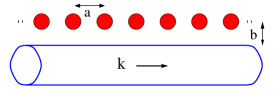
Figure 1: The atomic lattice of lattice constant $a$ is localized parallel to the nanofiber at distance $b$.

We consider a linear atomic lattice with one atom per site and lattice constant $a$. The atoms are taken to be of two-level systems with atomic transition $E_{A}$. The electronic excitation Hamiltonian is

$$H_{A}=E_{A}\sum_{n}B_{n}^{\dagger}B_{n},$$ (1)

where $B_{n}^{\dagger}$ and $B_{n}$ are the creation and annihilation operators of an excitation at atom $n$, and the operators are of spin half. In the present section as we deal with single excitation at most in the system we can assume the operators to be of bosons with the commutation relation $[B_{n},B_{m}^{\dagger}]=\delta_{nm}$. From symmetry consideration, in the limit of large number of lattice sites $N$, that is $N\gg 1$, where the periodic boundary condition makes sense, we can use the Fourier transform

$$B_{n}=\frac{1}{\sqrt{N}}\sum_{k}B_{k}e^{-ikz_{n}},$$ (2)

where the position of atom $n$ is $z_{n}=an$, with $n=0,\pm 1,\cdots,\pm M$, and $2M+1=N$. The wave number $k$ takes the values $k=\frac{2\pi}{Na}l$, with $l=0,\pm 1,\cdots,\pm M$. The Hamiltonian casts to

$$H_{A}=E_{A}\sum_{k}B_{k}^{\dagger}B_{k}.$$ (3)

The excited atom have a finite life time, e.g. the damping rate of the $D2$ transition of cesium atom at zero temperature is $5.2\ MHz$. Later the excited atom damping rate is included phenomenologically. Life times of electronic excitations in a lattice of atoms of finite size and in which the interatomic distance can be larger or of the order of the transition wavelength have been studied in ZoubiD . It is shown that the life time of excited atom is strongly affected by the existence of the other atoms in the lattice.

We consider one dimensional propagating photons, and to concentrate in the lowest fiber hybrid modes of $HE_{11}$. The photons are represented by the Hamiltonian

$$H_{C}=\sum_{q}\ E_{C}(q)\ a_{q}^{\dagger}a_{q},$$ (4)

where $a_{q}^{\dagger}$ and $a_{q}$ are the creation and annihilation operators of a photon of mode $q$. In order to define the values of the wave number $q$, we assume two parallel quantization mirrors, at the far sides of the long nanofiber, and that are separated by a distance $L$. Hence, using period boundary condition that allows propagating photons, the wave number $q$ is quantized and takes the values $q=2\pi l/L$, where $l=0,\pm 1,\pm 2,\cdots,\pm\infty$. The photon dispersion can be given by

$$E_{C}(q)=\frac{\hbar c}{\sqrt{\epsilon}}\sqrt{q_{0}^{2}+q^{2}},$$ (5)

where $\epsilon$ is an effective dielectric constant, and $q_{0}$ is the confinement wave number that absorb all the complexity arouses in the fiber photon dispersion. The fiber photons have relatively long life time, but they can be damped indirectly through their coupling to the atoms. The damping rate of the cavity photons is contained later phenomenologically.

The excitation-photon coupling is taken in the electric dipole approximation by $H_{I}=-\hat{\mbox{\boldmath$\mu$}}\cdot\hat{E}$, where the excitation transition dipole operator is given by $\hat{\mbox{\boldmath$\mu$}}=\mbox{\boldmath$\mu$}\sum_{n}\left(B_{n}+B_{n}^{\dagger}\right)$, and $\mu$ is the transition dipole. The photon electric field operator is given by

$$\hat{E}(r,z)=i\sum_{q}\sqrt{\frac{E_{C}(q)}{2\epsilon_{0}V}}{\bf e}u(r)\left(a_{q}e^{-iqz}-a_{q}^{\dagger}e^{iqz}\right),$$ (6)

where $V$ is the photon effective volume, ${\bf e}$ is the photon unit vector polarization, and $u(r)$ is the photon mode function that can contain all the complexity of the real fiber photon mode function.

The interaction Hamiltonian in the rotating wave approximation, and in the Schr$\ddot{o}$dinger picture, reads

$$H_{AC} = -i\sum_{qn}\sqrt{\frac{E_{C}(q)}{2\epsilon_{0}V}}u(b)(\mbox{\boldmath$\mu$}\cdot{\bf e})$$ (7)

$$\times \left(a_{q}B_{n}^{\dagger}e^{-iqz_{n}}-B_{n}a_{q}^{\dagger}e^{iqz_{n}}\right).$$

The electric field is taken at the atom positions with $u(b)$ the mode function at the lattice position that is separated by $b$ from the fiber. We consider here the case in which the fiber length is equal to the lattice length. Using the inverse of the above Fourier transform, and in using the known lattice identity $\frac{1}{N}\sum_{n}e^{i(q-k)z_{n}}=\delta_{kq}$, at the limit of $N\gg 1$, we get

$$H_{AC}=\sum_{k}\left(g_{k}\ a_{k}B_{k}^{\dagger}+g_{k}^{\star}\ B_{k}a_{k}^{\dagger}\right),$$ (8)

where we define the coupling parameter

$$g_{k}=-i\sqrt{\frac{E_{C}(k)N}{2\epsilon_{0}V}}u(b)(\mbox{\boldmath$\mu$}\cdot{\bf e}).$$ (9)

Due to translational symmetry the interaction is between an excitation and a photon with the same wave number.

The total Hamiltonian, as a results of exploiting the lattice symmetry, is separated for each $k$ and given by

$$H=\sum_{k}\left\{E_{A}\ B_{k}^{\dagger}B_{k}+E_{C}(k)\ a_{k}^{\dagger}a_{k}+g_{k}\ a_{k}B_{k}^{\dagger}+g_{k}^{\star}\ B_{k}a_{k}^{\dagger}\right\}.$$ (10)

The Hamiltonian also includes the term $H_{dec}=\sum_{q\neq k}E_{C}(q)\ a_{q}^{\dagger}a_{q}$, that represents all the photons which decouple to the excitations. For the case where the fiber length is exactly equal to the lattice length, that is $L=aN$, the last term represents all photons with half wave length smaller than the lattice constant, that is $a>\lambda/2$ where $q=2\pi/\lambda$. Or for photons with wave numbers larger than the Brillouin zone boundary, that is $q>k_{B}$ where $k_{B}=\pi/a$. As in the following we interest in excitation-photon resonances only at small wave numbers, with $k\ll k_{B}$, the last term photons are far off resonance with the atomic transition and they fall outside the first Brillouin zone boundary. Namely we have $E_{C}(k_{B})>E_{A}$. Hence we drop this term as it includes photons that are not involved in the dynamics.

On the other hand the fiber can naturally provide propagating evanescent fields only for modes with wavelengths larger than the tapered fiber radius, which is in the experiment about $250\ nm$, and all modes with wavelengths smaller than the fiber radius are concentrated inside the fiber, which is the case for the $HE_{11}$ modes that considered in the experiments Warken . As the lattice constant is about $500\ nm$, the number of effective photon modes is not much larger than the number of atom sites, the fact that supports our representation.

In the strong coupling regime where the excitation and photon line widths are smaller than the coupling parameter, the excitations and photons are coherently mixed to give two polariton branches. The Hamiltonian is diagonalized by using the upper and lower polariton operators

$$A_{k}^{\pm}=X_{k}^{\pm}\ B_{k}+Y_{k}^{\pm}\ a_{k},$$ (11)

which is a coherent superposition of excitations and photons. The mixing amplitudes are defined by

$$X_{k}^{\pm}=\pm\sqrt{\frac{D_{k}\mp\delta_{k}}{2D_{k}}},\ \ \ Y_{k}^{\pm}=\frac{g_{k}}{\sqrt{2D_{k}(D_{k}\mp\delta_{k})}},$$ (12)

where $D_{k}=\sqrt{\delta_{k}^{2}+|g_{k}|^{2}}$, and the detuning is $\delta_{k}=\frac{E_{C}(k)-E_{A}}{2}$. The polariton Hamiltonian reads

$$H_{pol}=\sum_{k,\nu}E_{\nu}(k)\ A_{k}^{\nu\dagger}A_{k}^{\nu},$$ (13)

with the polariton dispersions

$$E_{\pm}(k)=\frac{E_{C}(k)+E_{A}}{2}\pm D_{k}.$$ (14)

We present the results for some typical numbers. The transition energy is $E_{A}=1\ eV$, the lattice constant is $a=5000\ \AA$, the dielectric constant $\epsilon=4$, the transition dipole is $\mu=2\ e\AA$, and the mode function is estimated to be $u(b)=0.25$. We also use $V=SNa$ with the effective area $S=\pi a^{2}$. We have resonance excitation-photon at $k=0$, where $q_{0}\approx 10^{-3}\ \AA^{-1}$, with $E_{C}(0)=E_{A}$. The boundary of the Brillouin zone is at $k_{B}\approx 6.28\times 10^{-4}\ \AA^{-1}$ with photon energy of $E_{C}(k_{B})\approx 1.18\ eV$. Hence the photon at the Brillouin zone boundary are far off resonance with the atomic transition, where $E_{C}(k_{B})-E_{A}\approx 0.18\ eV$, that justifies the neglect of photons with wave numbers beyond $k_{B}$.

We plot the polariton eigen-energies for the two branches in figure (2.a) with their excitation and photon fractions in figure (2.b). The excitation and photon are coherently mix and split to give two polariton branches that are separated by the Rabi splitting at the intersection point. In the present zero detuning case we have Rabi splitting of $2|g_{0}|$, which is about $1.5\times 10^{-6}\ eV$ or $3.7\ GHz$. Around the excitation-photon intersection point, at $k=0$, the polariton is half excitation and half photon. For large $k$ the lower branch becomes excitation and the upper one photon.

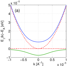
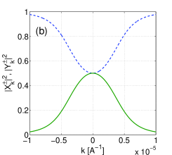
Figure 2: (a) The polariton relative energies $E_{\pm}(k)-E_{A}$ vs. $k$ for the upper and lower branches. The dashed lines are for the transition and the photon energies. (b) The excitation and photon fractions in the two polariton branches vs. $k$. In the lower branch the full line is for the photon fraction $|Y_{k}^{-}|^{2}$ and the dashed line for the excitation fraction $|X_{k}^{-}|^{2}$. In the upper branch the dashed line is for the photon fraction $|Y_{k}^{+}|^{2}$ and the full line for the excitation fraction $|X_{k}^{+}|^{2}$.

III Polariton-Polariton Kinematic Interactions

Electronic excitations are treated here as two level systems where the atomic operators are of spin-half. In the previous consideration we treated single excitation to appear at most in the system and the operators are assumed to be of bosons. For more excitations things start to be different as each atom can be excited only once by absorbing a photon. After the excitation the atom is saturated and the second photon will not be absorbed by the same excited atom.

First let us present the properties of spin-half operators on a lattice, $S_{n}^{\dagger}$ and $S_{n}$. They obey the fermi anti-commutation relation on the same site, that is

$$S_{n}S_{n}^{\dagger}+S_{n}^{\dagger}S_{n}=1\ ,\ S_{n}S_{n}=S_{n}^{\dagger}S_{n}^{\dagger}=0,$$ (15)

and the bose commutation relation between different sites, that is

$$\left[S_{n},S_{m}^{\dagger}\right]=\left[S_{n},S_{m}\right]=\left[S_{n}^{\dagger},S_{m}^{\dagger}\right]=0,\ (n\neq m).$$ (16)

Then spin-half operators on a lattice have mixed statistics. They are fermions on-site and bosons among different sites, where they usually termed paulions.

An exact transformation from paulions into bosons was suggested by Agranovich et al. Agranovich , in which each spin operator is represented in terms of infinite power series of boson operators. At low density of excitations, when the number of excitations is taken to be much smaller than the number of atoms in the system, it is a good approximation to keep the lowest terms of the series. Hence we have the transformation

$$S_{n}\rightarrow\left(1-B_{n}^{\dagger}B_{n}\right)B_{n}\ ,\ S_{n}^{\dagger}\rightarrow B_{n}^{\dagger}\left(1-B_{n}^{\dagger}B_{n}\right).$$ (17)

The transformation results in the previous boson Hamiltonian (10), and in the additional kinematic interaction Hamiltonian, as it is due to quantum statistics,

$$H_{I}=U\sum_{n}B_{n}^{\dagger}B_{n}^{\dagger}B_{n}B_{n},$$ (18)

where here $U=-E_{A}$. We neglect the interaction term results of the excitation-photon coupling, as we are in the limit of $E_{A}\gg|g_{k}|$. The present bosonization transforms the system from free paulions into interacting bosons. The interaction is on-site with parameter $E_{A}$. The interaction is attractive, but the formation of bound states is immaterial as it is of deep energy of $2E_{A}$ and no source avaliable to absorb such energy. Hence the interaction can lead only to scattering among the particles. In the hard-core boson model presented later we have the limit $U\rightarrow\infty$, and the above transformation becomes exact and hold for any density of excitations. The dynamical interactions due to electrostatic forces among neutral atoms are much smaller than the above kinematic ones at the present experimental interatomic distances.

In momentum space, by using the previous excitation operators, the interaction reads

$$H_{I}=\frac{U}{N}\sum_{kk^{\prime}\bar{k}}B_{k^{\prime}-\bar{k}}^{\dagger}B_{k+\bar{k}}^{\dagger}B_{k^{\prime}}B_{k}.$$ (19)

The next step is to write the interaction in terms of polariton operators, to get

$$H_{I}=\frac{U}{N}\sum_{kk^{\prime}\bar{k}}\sum_{rsuv}\left(X_{k}^{r\star}X_{k^{\prime}}^{s\star}X_{k+\bar{k}}^{u}X_{k^{\prime}-\bar{k}}^{v}\right)A_{k^{\prime}-\bar{k}}^{v\dagger}A_{k+\bar{k}}^{u\dagger}A_{k^{\prime}}^{s}A_{k}^{r}.$$ (20)

The Hamiltonian represents the interaction between two polaritons initially in branches $r$ and $s$ with momenta $k$ and $k^{\prime}$, and after the interaction in branches $u$ and $v$ with momenta $k+\bar{k}$ and $k^{\prime}-\bar{k}$, where they exchange momentum $\bar{k}$ and can also change branches.

Let us concentrate here in the interaction among lower branch polaritons. We assume the higher branch to be un-populated and we neglect the possibility of the scattering of two lower polaritons with final states in the upper branch. This process can be excluded due to conservation of energy and momentum. We treat polaritons with small wave numbers and around the minimum energy of the lower branch. These polaritons can be assumed to have a parabolic dispersion with a mass of the order of the cavity photon effective mass. Hence we can drop here the branch index. As $X_{k}$ are smooth functions of $k$ for small $k$ we can neglect the dependent of $X_{k}$ on $k$ and we use $X_{0}$. The interaction can be at any lattice site with the same probability of $1/N$. Finally we can write

$$H_{I}=\frac{a}{L}U|X_{0}|^{4}\sum_{kk^{\prime}\bar{k}}A_{k^{\prime}-\bar{k}}^{\dagger}A_{k+\bar{k}}^{\dagger}A_{k^{\prime}}A_{k},$$ (21)

where $|X_{0}|^{4}=\frac{\left(\sqrt{\delta_{0}^{2}+|g_{0}|^{2}}+\delta_{0}\right)^{2}}{4\left(\delta_{0}^{2}+|g_{0}|^{2}\right)}$, with $N=L/a$.

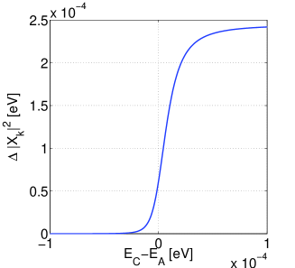
Figure 3: The scattering strength $\Delta|X_{k}|^{4}$ vs. the excitation-photon detuning $E_{C}(k)-E_{A}$, at $k=10^{-6}\ \AA^{-1}$.

In the hard core boson model the scattering length is exactly the potential range, which is for the lattice case the lattice constant $a$. In the next section we give detail calculation of the scattering problem that confirm using the hard-core boson model. For large wavelength polaritons, the interaction strength $U$ can be represented in term of the scattering length Dalibard , by $U=\frac{4\pi\hbar^{2}}{m_{eff}a^{2}}$, where $m_{eff}$ is the polariton effective mass that can be defined by $\frac{1}{m_{eff}}=\frac{1}{\hbar^{2}}\frac{\partial^{2}E_{\nu}(k)}{\partial k^{2}}$. Hence we get the effective interaction Hamiltonian

$$H_{I}=\Delta\sum_{rsuv}\sum_{kk^{\prime}\bar{k}}\left(X_{k}^{r\star}X_{k^{\prime}}^{s\star}X_{k+\bar{k}}^{u}X_{k^{\prime}-\bar{k}}^{v}\right)A_{k^{\prime}-\bar{k}}^{v\dagger}A_{k+\bar{k}}^{u\dagger}A_{k^{\prime}}^{s}A_{k}^{r},$$ (22)

where $\Delta=\frac{4\pi\hbar^{2}}{m_{eff}aL}$. For the lower polariton branch around small wave numbers, $m_{eff}$ is of the order of the photon effective mass. We can write

$$H_{I}=\Delta|X_{0}|^{4}\sum_{kk^{\prime}\bar{k}}A_{k^{\prime}-\bar{k}}^{\dagger}A_{k+\bar{k}}^{\dagger}A_{k^{\prime}}A_{k}.$$ (23)

In using the previous numbers, in figure (3) we plot the effective interaction as a function of the excitation-photon detuning for a fixed wave number of $k=10^{-6}\ \AA^{-1}$. We take the lattice length to be $L=1\ mm$. The photon effective mass is about $m_{eff}c^{2}=4eV$. It is clear that the interaction strength is strong around zero detuning and decreased with increasing the negative detuning.

We conclude here that the excitation-photon detuning serves as a significant control parameter for the strength of the kinematic interaction. By varying the detuning from being positive where polaritons are mainly excitations into positive where they are mainly photons, the polaritons switch from strongly interacting quasi-particles into weakly interacting ones. For a fixed fiber properties, the atomic excitation level can be changed in applying external fields.

We examine now the validity of considering the system of polaritons as a dilute degenerate bose gas. The inter-polariton separation needs to be of the order of the de Broglie thermal wavelength, that is defined by Dalfovo $\lambda_{dB}=\sqrt{\frac{2\pi\hbar^{2}}{m_{pol}k_{B}T}}$. For interacting polaritons the dilute Bose gas limit is for de Broglie wave length much larger than the interaction range, that is $\lambda_{dB}\gg a$. Using the previous numbers at resonance where $m_{pol}c^{2}\approx 4\ eV$ and at room temperature, that is $k_{B}T\approx 25\ meV$, we get $\lambda_{dB}\approx 15\times 10^{3}\ \AA$, which is a bit larger than $a=5\times 10^{3}\ \AA$. Hence one needs either smaller lattice constant or to go to lower temperatures. At temperature of $T=25\ K$ we have $k_{B}T\approx 2.5\ meV$ and we get $\lambda_{dB}\approx 5\times 10^{4}\ \AA$ which is one order of magnitude larger than $a$.

The polariton effective mass for small wave numbers is of the order of the cavity photon effective mass at small wave numbers. For small wave number photons, or long wave length ones, in the limit $q\ll q_{0}$, we have $E_{C}(q)\approx E_{0}+\frac{\hbar^{2}q^{2}}{2m_{C}}$, where $E_{0}=\frac{\hbar cq_{0}}{\sqrt{\epsilon}}$, and we defined the confined photon effective mass $m_{C}c^{2}=\hbar cq_{0}\sqrt{\epsilon}$. The dispersion is parabolic with finite zero energy of $E_{0}$, the fact that has big influence on the system properties that treated later.

This discussion is a step toward achieving BEC of polaritons in such system, which is possible due to the small effective mass and the finite minimum energy. Thermalization of polaritons toward the minimum energy is a critical issue here and can be achieved through polariton-polariton kinematic interactions. This topic needs much more study that we leave for the future.

IV Backward and Forward Scattering of Polaritons

Let us now examine the scattering problem of two polaritons via the kinematic interaction, where the scattering is only among the polariton excitation parts. We consider analytically the scattering of lower branch polaritons with small wave numbers. Here we neglect the scattering of lower polaritons into upper ones as final states, that can be justified due to conservation of energy and momentum, but the upper polaritons still appear as intermediate scattering states. This case is of a single channel scattering problem, and we can use well known results of scattering theory. In the center of mass frame the problem is equivalent to the scattering of a polariton with reduced effective mass from the potential results of the other polariton, which is equivalent to the scattering of a polariton from an effective potential that can be modeled as a defect in the lattice Baym ; Newton .

For the scattering of a polariton from a defect, we assume that single atom is missed in the ideal lattice as in figure (4). Namely we have a localized vacancy at the origin site $n=0$. We add and subtract atomic Hamiltonian part at the vacancy site to get the above free polariton Hamiltonian $H_{pol}$ with additional impurity Hamiltonian, that is we have $H=H_{pol}+H_{v}$ where $H_{v}=U\ B_{0}^{\dagger}B_{0}$. The vacancy appears as potential well of depth $E_{A}$ and width $a$. We will not try to diagonalize the whole Hamiltonian, but we will treat the elastic scattering problem.

Figure 4: A lattice of lattice constant $a$ with a localized vacancy.

The polariton eigenstates obey $H_{pol}|\phi^{pol}_{{k}\nu}\rangle=E_{\nu}(k)|\phi^{pol}_{{k}\nu}\rangle$, and the whole system eigenstates obey $H|\psi\rangle=E|\psi\rangle$. The cavity photon eigenstate is defined by $a_{k}^{\dagger}|vac\rangle=|\phi_{k}^{ph}\rangle$, and the excitation eigenstate in quasi-momentum space is defined by $B_{k}^{\dagger}|vac\rangle=|\phi_{k}^{ex}\rangle$. The $\nu$ polariton branch eigenstate is defined by $A_{{k}\nu}^{\dagger}|vac\rangle=|\phi_{{k}\nu}^{pol}\rangle$, and in terms of excitation and photon states we get $|\phi_{{k}\pm}^{pol}\rangle=X_{k}^{\pm}\ |\phi_{k}^{ex}\rangle+Y_{k}^{\pm}\ |\phi_{k}^{ph}\rangle$. In terms of real lattice space, we get $|\phi_{{k}\pm}^{pol}\rangle=\frac{X_{k}^{\pm}}{\sqrt{N}}\sum_{n}e^{ikz_{n}}\ |\phi_{n}^{ex}\rangle+Y_{k}^{\pm}\ |\phi_{k}^{ph}\rangle$. A general state $|\psi\rangle$ can be expanded as $|\psi\rangle=\sum_{k}\psi_{k}^{ph}\ |\phi_{k}^{ph}\rangle+\sum_{m}\psi_{m}^{ex}\ |\phi_{m}^{ex}\rangle$.

In the scattering problem the incoming polariton is prepared very far from the impurity in the unperturbed state $|\phi_{{k}\nu}^{pol}\rangle$ and the scattered polariton is observed very far from the impurity. Hence, the whole system eigenstates $|\psi\rangle$ needs to obey the boundary condition $|\psi\rangle\rightarrow|\phi_{{k}\nu}^{pol}\rangle$ as $H_{v}\rightarrow 0$. The required solution is given by the Schwinger-Lippmann equation Newton

$$|\psi\rangle=|\phi_{{k}\nu}^{pol}\rangle+G_{0}H_{v}|\psi\rangle,$$ (24)

where

$$G_{0}=\lim_{\eta\rightarrow 0_{+}}\left(\frac{1}{E-H_{0}+i\eta}\right).$$ (25)

The sign of $+i\eta$ is chosen in such a way to ensure that the scattered polariton propagates far from the impurity.

We multiply the equation from the left by the lattice excitation eigenstate $\langle\phi_{n}^{ex}|$, and insert the identity operator, $\sum_{m}|\phi_{m}^{ex}\rangle\langle\phi_{m}^{ex}|=\hat{\bf 1}$, between $G_{0}$ and $H_{v}$, to get

$$\langle\phi_{n}^{ex}|\psi\rangle=\langle\phi_{n}^{ex}|\phi^{pol}_{{k}\nu}\rangle+\sum_{m}\langle\phi_{n}^{ex}|G_{0}|\phi_{m}^{ex}\rangle\langle\phi_{m}^{ex}|H_{v}|\psi\rangle.$$ (26)

Using the above definitions, we get the scattered polariton excitation part amplitude by

$$\psi_{n}^{ex}=\frac{X_{k}^{\nu}}{\sqrt{N}}e^{ikz_{n}}+\frac{U}{N}\sum_{{k^{\prime}}\mu}\lim_{\eta\rightarrow 0_{+}}\frac{|X_{k^{\prime}}^{\mu}|^{2}\ e^{i{k^{\prime}z_{n}}}}{E_{\nu}(k)-E_{\mu}(k^{\prime})+i\eta}\ \psi_{0}^{ex},$$ (27)

where due to energy conservation we replaced the energy $E$ by the initial energy $E_{\nu}(k)$. For the impurity site amplitude we have

$$\psi_{0}^{ex}=\frac{X_{k}^{\nu}}{\sqrt{N}}\left\{1-\frac{U}{N}\sum_{{k^{\prime}}{\mu}}\lim_{\eta\rightarrow 0_{+}}\frac{|X_{k^{\prime}}^{\mu}|^{2}}{E_{\nu}(k)-E_{\mu}(k^{\prime})+i\eta}\right\}^{-1}.$$ (28)

We thus obtain

$$\psi_{n}^{ex}=\frac{X_{k}^{\nu}}{\sqrt{N}}\left\{e^{i{kz}_{n}}-\frac{UI_{O}}{1+UI_{S}}\right\}.$$ (29)

For simplicity, at large number of lattice sites, the $k$-space can be assumed continuous and the sums converted to the integral $\frac{1}{N}\sum_{k^{\prime}}\rightarrow\frac{a}{2\pi}\int dk^{\prime}$, we get

$$I_{O} = \sum_{\mu}\frac{aU}{2\pi}\int dk^{\prime}\lim_{\eta\rightarrow 0_{+}}\frac{|X_{k^{\prime}}^{\mu}|^{2}\ e^{i{k^{\prime}z}_{n}}}{E_{\nu}(k)-E_{\mu}(k^{\prime})+i\eta},$$

$$I_{S} = \sum_{\mu}\frac{aU}{2\pi}\int dk^{\prime}\lim_{\eta\rightarrow 0_{+}}\frac{|X_{k^{\prime}}^{\mu}|^{2}}{E_{\nu}(k)-E_{\mu}(k^{\prime})+i\eta}.$$

We calculate here analytically the scattering case with small wave number polaritons, where one can approximate the dispersion to be parabolic around $k\approx 0$, where we have $E_{-}(k)\approx E_{-}(0)+\frac{\hbar^{2}k^{2}}{2m_{pol}}$, and we defined the polariton effective mass around $k\approx 0$. In the case of excitation-photon close to resonance it is of the order of the cavity photon effective mass. We also neglect the contribution of the upper branch polaritons as intermediate states in the scattering. They are of higher energy and their excitation fraction become smaller and smaller with increasing $k$. Here the integrals cast into

$$I_{O} = \frac{aU}{2\pi}\frac{2m_{pol}}{\hbar^{2}}\int dk^{\prime}\lim_{\eta\rightarrow 0_{+}}\frac{|X_{k^{\prime}}^{-}|^{2}\ e^{i{k^{\prime}z}_{n}}}{k^{2}-{k^{\prime}}^{2}+i\eta},$$

$$I_{S} = \frac{aU}{2\pi}\frac{2m_{pol}}{\hbar^{2}}\int dk^{\prime}\lim_{\eta\rightarrow 0_{+}}\frac{|X_{k^{\prime}}^{-}|^{2}}{k^{2}-{k^{\prime}}^{2}+i\eta}.$$

The calculus of residue yields

$$I_{O}=iU\frac{am_{pol}}{\hbar^{2}k}|X_{k}^{-}|^{2}\ e^{-i{kz}_{n}},\ \ \ I_{S}=iU\frac{am_{pol}}{\hbar^{2}k}|X_{k}^{-}|^{2}.$$ (32)

We write

$$\psi_{n}^{ex}=\frac{X_{k}^{\nu}}{\sqrt{N}}\left\{e^{i{kz}_{n}}+f(k)e^{-ikz_{n}}\right\},$$ (33)

where we defined the scattering amplitude by

$$f(k)=\frac{i\frac{U}{\Lambda}\left(\frac{\pi^{2}}{2ka}\right)|X_{k}^{-}|^{2}}{1-i\frac{U}{\Lambda}\left(\frac{\pi^{2}}{2ka}\right)|X_{k}^{-}|^{2}},$$ (34)

and we defined the energy $\Lambda=\frac{\hbar^{2}\pi^{2}}{2a^{2}m_{pol}}$. The square absolute value is given by

$$|f(k)|^{2}=\frac{\frac{U^{2}}{\Lambda^{2}}\left(\frac{\pi^{2}}{2ka}\right)^{2}|X_{k}^{-}|^{4}}{1+\frac{U^{2}}{\Lambda^{2}}\left(\frac{\pi^{2}}{2ka}\right)^{2}|X_{k}^{-}|^{4}}.$$ (35)

As $U\gg\Lambda$, the excitation part scattering of small wave vector lower polaritons is complete with $|f(k)|^{2}\approx 1$. We conclude that the polariton reflection is $|X_{k}^{-}|^{2}$ and the polariton transmission is $|Y_{k}^{-}|^{2}$. One need to worry about the case of large positive detuning as the parabolic assumption breaks down and numerical calculation is needed, but the conclusion is the same. We obtain

$$\psi_{n}^{ex}=\frac{X_{k}^{\nu}}{\sqrt{N}}\left\{e^{i{kz}_{n}}-e^{-ikz_{n}}\right\}.$$ (36)

We showed that the reflection amplitude is exactly the excitation amplitude and the transmission amplitude is the photon amplitude for the scatterer polaritons. The results of this limit is exactly that of the scattering from a hard core potential of radius $a$, where it is in the limit of $U\rightarrow\infty$ for the defect potential, and that verifies the use of the hard-core boson model in the present context. In the appendix we implement the above result to the scattering of polaritons from an impurity consists of an atom of a different type in the lattice.

The above conclusion can be easily generalized to the scattering of any pair of polaritons with any wave numbers and in any branches. Careful inspection of the polariton excitation part scattering amplitude reveals the fact that the polariton excitation parts of two polaritons can be only back scattered, in the one dimensional case. This fact is due to the large value of $U$ relative to the other system parameters, and much more strongly, in the hard-core boson model this conclusion is exact. Hence if we consider two incident polaritons with wave numbers $k_{1}$ and $k_{2}$ and in polariton branches $r$ and $s$, respectively, the scattered polaritons are with wave numbers $k_{1}^{\prime}$ and $k_{2}^{\prime}$, and in the branches $r^{\prime}$ and $s^{\prime}$, where the elastic scattering respects conservation of energy and momentum

$$E_{r}(k_{1})+E_{s}(k_{2})=E_{r^{\prime}}(k_{1}^{\prime})+E_{s^{\prime}}(k_{2}^{\prime}),\ |k_{1}+k_{2}|=|k_{1}^{\prime}+k_{2}^{\prime}|.$$ (37)

The scattering is represented by the scattering matrix

$$\left(\begin{array}[]{cc}A_{k_{1}^{\prime}}^{r^{\prime}}\\ A_{k_{2}^{\prime}}^{s^{\prime}}\end{array}\right)=\left(\begin{array}[]{ccc}X_{k_{1}}^{r}&Y^{s}_{k_{2}}\\ Y^{r}_{k_{1}}&X_{k_{2}}^{s}\end{array}\right)\left(\begin{array}[]{cc}A_{k_{1}}^{r}\\ A_{k_{2}}^{s}\end{array}\right).$$ (38)

The scattering process is plotted in figure (5).

For the lower branch polaritons around small wave numbers the dispersion is parabolic with an effective mass, hence the conservation of energy condition becomes $k_{1}^{2}+k_{2}^{2}=k_{1}^{\prime 2}+k_{2}^{\prime 2}$. We have only two possible scattering channels: forward scattering with $k_{1}=k_{2}^{\prime}$ and $k_{2}=k_{1}^{\prime}$, or backward scattering with $k_{1}=k_{1}^{\prime}$ and $k_{2}=k_{2}^{\prime}$. The process can lead to the formation of entangled polaritons discriminated by their wave numbers. For two incident polaritons with $k_{1}$ and $k_{2}$ in the lower branch, we get the final entangled state $|Ent(k_{1},k_{2})\rangle=Y_{k_{1}}Y_{k_{2}}|k_{1},k_{2}\rangle+X_{k_{1}}X_{k_{2}}|k_{2},k_{1}\rangle$.

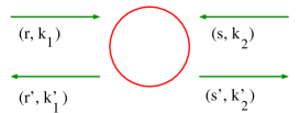
Figure 5: Schematic plot of two incident polaritons $(r,k_{1})$ and $(s,k_{2})$, scattered into final polaritons $(r^{\prime},k_{1}^{\prime})$ and $(s^{\prime},k_{2}^{\prime})$.

Polaritons in the case of large negative detuning are weakly interact and can form a superfluid. In this limit as the polaritons are mainly photons we can treat them as interacting photons and there is a place to examine the superfluidity of photons. The main reasons that allow us to consider the superfluidity of photons are: First as polaritons include very small component of excitation they become interacting particles. Second we dealing here with confined photons and they have effective mass and non-zero energy at zero wave number. The only point to worry about is the finite life time of polaritons which is due to the life time of the photons and the excited atoms.

These features are important toward achieving the superfluidity of photons. The finite minimum energy needs to be larger than the thermal energy as then the disappearance of photons within the cavity can be negligible and one get finite photon chemical potential, which is important for defining conserved number of photons in the system. Using the Bogoliubov theory for a dilute Bose gas, the elementary excitation spectrum of the superfluid of photons is linear with sound wave excitations. The sound waves are found to be Dalfovo ; Chiao $v_{s}=\sqrt{\frac{N_{0}}{N}\frac{2\bar{U}}{m_{pol}c^{2}}}c$, where here $N_{0}$ is the number of condensate polaritons, $N$ the total number of lattice sites, and $\bar{U}$ is an effective polariton-polariton potential that can be extracted from the above scattering amplitudes. We use the previous effective potential of $\bar{U}=\Delta|X_{k}|^{4}$.

V Polariton Nonlinear Optical Processes

We aim now to apply the polariton-polariton kinematic interaction as a mechanism for nonlinear optical processes Boyd , and that provide a direct observation tool for the strength of the above kinematic interaction. We start by formal discussion in deriving the mean field equations of motion and including the damping rates phenomenologically with the coupling to external fields, and later we concentrate in few specific cases. The interacting polariton Hamiltonian reads

$$H=\sum_{k,r}E_{r}(k)\ A_{k}^{r\dagger}A_{k}^{r}+\sum_{rsuv}\sum_{k,k^{\prime},\bar{k}}U^{rsuv}_{k,k^{\prime},\bar{k}}\ A_{k^{\prime}-\bar{k}}^{v\dagger}A_{k+\bar{k}}^{u\dagger}A_{k^{\prime}}^{s}A_{k}^{r},$$ (39)

where $U^{rsuv}_{k,k^{\prime},\bar{k}}=\Delta\ \left(X_{k}^{r\star}X_{k^{\prime}}^{s\star}X_{k+\bar{k}}^{u}X_{k^{\prime}-\bar{k}}^{v}\right)$.

The equation of motion for the polariton operator, in the Heisenberg picture, is given by $i\hbar\frac{d}{dt}A_{k^{\prime\prime}}^{w}=[A_{k^{\prime\prime}}^{w},H]$, that yields

$$i\frac{d}{dt}A_{k^{\prime\prime}}^{w} = \left(\Omega_{k^{\prime\prime}}^{w}-i\Gamma_{k^{\prime\prime}}^{w}\right)A_{k^{\prime\prime}}^{w}+F_{k^{\prime\prime}}^{w}$$

$$+ \sum_{rsu}\sum_{k,k^{\prime}}V^{rsuw}_{k,k^{\prime},k^{\prime\prime}}\ A_{k+k^{\prime}-k^{\prime\prime}}^{u\dagger}A_{k^{\prime}}^{s}A_{k}^{r}.$$

We used $E_{r}(k)=\hbar\Omega_{k}^{r}$, and defined $\hbar V^{rsuw}_{k,k^{\prime},k^{\prime\prime}}=U^{rsuw}_{k,k^{\prime},k^{\prime}-k^{\prime\prime}}+U^{rswu}_{k,k^{\prime},k^{\prime\prime}-k}$. The polariton damping rate $\Gamma_{k}^{r}$, of branch $r$ and wave number $k$, is included phenomenologically. It is a good approximation when the thermal energy is much smaller than the polariton energy. The damping is due to the life times of both the fiber photons and the excited atoms, where we can write

$$\Gamma_{k}^{r}=\frac{\Gamma_{A}}{2}|X_{k}^{r}|^{2}+\frac{\Gamma_{C}}{2}|Y_{k}^{r}|^{2},$$ (41)

with $\Gamma_{A}$ is the excited atom damping rate, and $\Gamma_{C}$ is the fiber photon damping rate.

Furthermore, we include in the equation of motion external pump of polaritons, $F_{k}^{r}$, at branch $r$ and wave number $k$. We consider external pumps at the two far edges of the fiber, by assuming effective mirrors at the far sides of the fiber that couple the fiber photon to external pump fields. Namely we have the Hamiltonian $H_{ex}=\hbar\gamma\sum_{k}\left(a_{k}\mathcal{F}^{\ast}_{k}+a_{k}^{\dagger}\mathcal{F}_{k}\right)$, where $\gamma$ is the coupling parameter at the mirrors, and $\mathcal{F}_{k}$ is the external classical field of wave number $k$. In term of polaritons, by using the inverse transformation $a_{k}=\sum_{r}Y_{k}^{r\ast}A_{k}^{r}$, we obtain $H_{ex}=\hbar\sum_{k,r}\left(F^{r\star}_{k}A_{k}^{r}+F^{r}_{k}A_{k}^{r\dagger}\right)$, where we defined $F^{r}_{k}=\gamma Y_{k}^{r\ast}\mathcal{F}_{k}$. This Hamiltonian leads to the external field term in the above equation of motion.

We concentrate mainly in lower branch polaritons, and we drop the branch indices. Then we have

$$i\frac{d}{dt}A_{k^{\prime\prime}} = \left(\Omega_{k^{\prime\prime}}-i\Gamma_{k^{\prime\prime}}\right)A_{k^{\prime\prime}}$$ (42)

$$+ \sum_{k,k^{\prime}}V_{k,k^{\prime},k^{\prime\prime}}\ A_{k+k^{\prime}-k^{\prime\prime}}^{\dagger}A_{k^{\prime}}A_{k}+F_{k^{\prime\prime}}.$$

We consider only polaritons of two fixed wave numbers, $k_{1}$ and $k_{2}$. As we discussed before due to conservation of energy and momentum, we have only two possible channels: (i) forward scattering $(k_{1},k_{2})\rightarrow(k_{1},k_{2})$, and (ii) backward scattering $(k_{1},k_{2})\rightarrow(k_{2},k_{1})$. We obtain the two equations of motion

$$i\frac{d}{dt}A_{k_{1}} = \left(\Omega_{k_{1}}-i\Gamma_{k_{1}}\right)A_{k_{1}}+V_{k_{1},k_{2}}\ A_{k_{2}}^{\dagger}A_{k_{2}}A_{k_{1}}+F_{k_{1}},$$

$$i\frac{d}{dt}A_{k_{2}} = \left(\Omega_{k_{2}}-i\Gamma_{k_{2}}\right)A_{k_{2}}+V_{k_{1},k_{2}}\ A_{k_{1}}^{\dagger}A_{k_{1}}A_{k_{2}}+F_{k_{2}},$$

where $\hbar V_{k_{1},k_{2}}=2\Delta|X_{k_{1}}|^{2}|X_{k_{2}}|^{2}$.

The two external fields are oscillating with frequencies $\omega_{1}$ and $\omega_{2}$. Namely

$$F_{k_{1}}=\tilde{F}_{k_{1}}e^{-i\omega_{1}t},\ F_{k_{2}}=\tilde{F}_{k_{2}}e^{-i\omega_{2}t},$$ (44)

and the polaritons oscillate with the same frequencies

$$A_{k_{1}}=\tilde{A}_{k_{1}}e^{-i\omega_{1}t},\ A_{k_{2}}=\tilde{A}_{k_{2}}e^{-i\omega_{2}t},$$ (45)

which yield equations of motion in rotating frames

$$i\frac{d}{dt}\tilde{A}_{k_{1}} = \left(\Omega_{k_{1}}-\omega_{1}-i\Gamma_{k_{1}}\right)\tilde{A}_{k_{1}}$$

$$+ V_{k_{1},k_{2}}\ \tilde{A}_{k_{2}}^{\dagger}\tilde{A}_{k_{2}}\tilde{A}_{k_{1}}+\tilde{F}_{k_{1}},$$

$$i\frac{d}{dt}\tilde{A}_{k_{2}} = \left(\Omega_{k_{2}}-\omega_{2}-i\Gamma_{k_{2}}\right)\tilde{A}_{k_{2}}$$ (46)

$$+ V_{k_{1},k_{2}}\ \tilde{A}_{k_{1}}^{\dagger}\tilde{A}_{k_{1}}\tilde{A}_{k_{2}}+\tilde{F}_{k_{2}}.$$

At this point we apply the mean field theory by defining the expectation value of the polariton operators by $\tilde{\mathcal{A}}_{k_{1}}=\langle\tilde{A}_{k_{1}}\rangle$, and $\tilde{\mathcal{A}}_{k_{2}}=\langle\tilde{A}_{k_{2}}\rangle$. Moreover we apply the factorization approximation, in the mean field, $\langle\tilde{A}_{k_{2}}^{\dagger}\tilde{A}_{k_{2}}\tilde{A}_{k_{1}}\rangle=\langle\tilde{A}_{k_{2}}^{\dagger}\tilde{A}_{k_{2}}\rangle\langle\tilde{A}_{k_{1}}\rangle$ and $\langle\tilde{A}_{k_{1}}^{\dagger}\tilde{A}_{k_{1}}\tilde{A}_{k_{2}}\rangle=\langle\tilde{A}_{k_{1}}^{\dagger}\tilde{A}_{k_{1}}\rangle\langle\tilde{A}_{k_{2}}\rangle$. We can write $\langle\tilde{A}_{k_{2}}^{\dagger}\tilde{A}_{k_{2}}\tilde{A}_{k_{1}}\rangle=\mathcal{N}_{k_{2}}\tilde{\mathcal{A}}_{k_{1}}$ and $\langle\tilde{A}_{k_{1}}^{\dagger}\tilde{A}_{k_{1}}\tilde{A}_{k_{2}}\rangle=\mathcal{N}_{k_{1}}\tilde{\mathcal{A}}_{k_{2}}$, where we defined the expectation value of the number operators by $\mathcal{N}_{k_{1}}=\langle\tilde{A}_{k_{1}}^{\dagger}\tilde{A}_{k_{1}}\rangle$ and $\mathcal{N}_{k_{2}}=\langle\tilde{A}_{k_{2}}^{\dagger}\tilde{A}_{k_{2}}\rangle$. The equations of motion cast into

$$i\frac{d}{dt}\tilde{\mathcal{A}}_{k_{1}} = \left(\Omega_{k_{1}}-\omega_{1}-i\Gamma_{k_{1}}+V_{k_{1},k_{2}}\mathcal{N}_{k_{2}}\right)\tilde{\mathcal{A}}_{k_{1}}+\tilde{F}_{k_{1}},$$

$$i\frac{d}{dt}\tilde{\mathcal{A}}_{k_{2}} = \left(\Omega_{k_{2}}-\omega_{2}-i\Gamma_{k_{2}}+V_{k_{1},k_{2}}\mathcal{N}_{k_{1}}\right)\tilde{\mathcal{A}}_{k_{2}}+\tilde{F}_{k_{2}}.$$

The steady state solutions are obtained at $i\frac{d}{dt}\tilde{\mathcal{A}}_{k_{1}}=i\frac{d}{dt}\tilde{\mathcal{A}}_{k_{2}}=0$. Hence the steady state average number of polaritons, in the mean field theory, can be defined by $\mathcal{N}_{k_{1}}^{st}=|\tilde{\mathcal{A}}_{k_{1}}^{st}|^{2}$ and $\mathcal{N}_{k_{2}}^{st}=|\tilde{\mathcal{A}}_{k_{2}}^{st}|^{2}$, and that are given by

$$\mathcal{N}_{k_{1}}^{st} = \frac{|\tilde{F}_{k_{1}}|^{2}}{\left(\omega_{1}-\Omega_{k_{1}}-V_{k_{1},k_{2}}\mathcal{N}_{k_{2}}^{st}\right)^{2}+\Gamma_{k_{1}}^{2}},$$ (48)

$$\mathcal{N}_{k_{2}}^{st} = \frac{|\tilde{F}_{k_{2}}|^{2}}{\left(\omega_{2}-\Omega_{k_{2}}-V_{k_{1},k_{2}}\mathcal{N}_{k_{1}}^{st}\right)^{2}+\Gamma_{k_{2}}^{2}},$$

and which can be solved for $\mathcal{N}_{k_{1}}^{st}$ and $\mathcal{N}_{k_{2}}^{st}$.

We treat now pump-probe experiments in which one of the fields is taken to be strong and in resonance where $\omega_{1}=\Omega_{k_{1}}$ and that called the pump field, say the one with $k_{1}$, and results in a fixed $\mathcal{N}_{k_{1}}^{pump}$. The second field with $k_{2}$ is the weak probe field of $\tilde{F}_{k_{2}}^{probe}$, and that oscillates in frequency $\omega_{2}=\omega$, with the average number of polaritons

$$\mathcal{N}_{k_{2}}^{st}=\frac{|\tilde{F}_{k_{2}}^{probe}|^{2}}{\left(\omega-\Omega_{k_{2}}-V_{k_{1},k_{2}}\mathcal{N}_{k_{1}}^{pump}\right)^{2}+\Gamma_{k_{2}}^{2}}.$$ (49)

The spectrum can be obtained by changing $\omega$. The observed spectrum is a tool for evaluating the interaction strength. The blue shift in the probe spectrum is proportional to the interaction strength at a fixed pump.

We plot the probe spectrum for the cases with and without a pump, in which $\mathcal{N}_{k_{2}}^{st}(0)=\frac{|\tilde{F}_{k_{2}}^{probe}|^{2}}{\left(\omega-\Omega_{k_{2}}\right)^{2}+\Gamma_{k_{2}}^{2}}$. We use the previous numbers, and for the excited atom damping rate we have $\hbar\Gamma_{A}=2.15\times 10^{-8}\ eV$, and for the cavity photon damping rate we take $\hbar\Gamma_{C}=2.15\times 10^{-10}\ eV$. The average number of pump polaritons is taken to be $\mathcal{N}_{k_{1}}^{pump}=100$. We plot the scaled $\mathcal{N}_{k_{2}}^{st}/|\tilde{F}_{k_{2}}^{probe}|^{2}$ for arbitrary units as a function of the detuning $\omega-\Omega_{k_{2}}$, at $k_{2}=10^{-6}\ \AA^{-1}$. Figure (6.a) is for the zero excitation-photon detuning case with $E_{C}(k)-E_{A}=0$, and figure (6.b) for the detuning of $E_{C}(k)-E_{A}=-10^{-4}\ eV$. The shift in the probe spectrum after switching on the pump field can be used to extract the strength of the interaction for given average number of pump polaritons. It is clear that for larger negative detuning the shift is much smaller than the zero detuning case, as here the polaritons are much more photonic and weakly interact. Moreover, the scattering through the kinematic interaction significantly reduce the probe polariton intensity at the two cases.

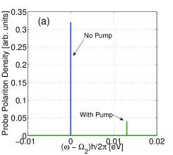
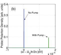
Figure 6: (a) The density of probe polaritons, with arbitrary units, as a function of the detuning $\omega-\Omega_{k_{2}}$, for $k_{2}=10^{-6}\ \AA^{-1}$. (a) At zero atom-photon detuning, that is $E_{C}(k)-E_{A}=0$. (b) At finite atom-photon detuning of $E_{C}(k)-E_{A}=-10^{-4}\ eV$.

Now we consider the case of two identical counter propagating resonance external fields of $\tilde{F}_{k_{1}}=\tilde{F}_{k_{2}}=\tilde{F}$, where $\omega_{1}=\Omega_{k_{1}}$ and $\omega_{2}=\Omega_{k_{2}}$, with $\Omega_{k_{1}}=\Omega_{k_{2}}=\Omega$ and $\Gamma_{k_{1}}=\Gamma_{k_{2}}=\Gamma$. We have $k_{1}=+k$ and $k_{1}=-k$. This fact leads to a fixed $\mathcal{N}_{k_{1}}=\mathcal{N}_{k_{2}}=\mathcal{N}$. At steady state $\tilde{\mathcal{A}}_{+k}^{st}=\tilde{\mathcal{A}}_{-k}^{st}=\frac{\tilde{F}}{i\Gamma-V\mathcal{N}}$, where $V=V_{k_{1},k_{2}}$. We have $\mathcal{N}=|\tilde{\mathcal{A}}_{+k}^{st}|^{2}=|\tilde{\mathcal{A}}_{-k}^{st}|^{2}=\tilde{\mathcal{A}}_{+k}^{st\star}\tilde{\mathcal{A}}_{-k}^{st}=\tilde{\mathcal{A}}_{-k}^{st\star}\tilde{\mathcal{A}}_{+k}^{st}$, with

$$\mathcal{N}(\Gamma^{2}+V^{2}\mathcal{N}^{2})=|\tilde{F}|^{2},$$ (50)

that needs to be solved for $\mathcal{N}$. In figure (7) we plot the average polariton number $\mathcal{N}$ as a function of the scaled external field intensity $|\tilde{F}|^{2}$ in using the previous numbers, and for zero excitation-photon detuning, that is $E_{C}(k)-E_{A}=0$, at $k=10^{-6}\ \AA^{-1}$. The finite detuning case of $E_{C}(k)-E_{A}=-10^{-5}\ eV$ is also plotted. It is easier to achieve higher average number of polaritons at fixed external field for the case of finite detuning than in the case of zero detuning.

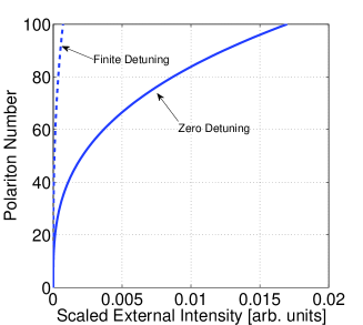
Figure 7: The average polariton number $\mathcal{N}$ vs. the scaled external field $|\tilde{F}|^{2}$, at zero atom-photon detuning, $E_{C}(k)-E_{A}=0$, and with $k=10^{-6}\ \AA^{-1}$. The dashed line is for the case of finite detuning with $E_{C}(k)-E_{A}=-10^{-5}\ eV$.

At this point we aim to calculate the correlation among two atoms setting at different sites in the lattice, which are $(n)$ and $(m)$. Namely, we target to calculate $\langle B_{m}^{\dagger}B_{n}\rangle$. But first we present the excitation operator in terms of polariton ones by $B_{n}=\frac{1}{\sqrt{N}}\sum_{k,r}X_{k}^{r}e^{-ikz_{n}}A_{k}^{r}$. For the present case we have

$$B_{n}=\frac{1}{\sqrt{N}}\left\{X_{+k}e^{-ikz_{n}}A_{+k}+X_{-k}e^{ikz_{n}}A_{-k}\right\}.$$ (51)

We have also $X_{+k}=X_{-k}=X$, and we get

$$\langle B_{m}^{\dagger}B_{n}\rangle = \frac{|X|^{2}}{N}\left\{\langle A_{+k}^{\dagger}A_{+k}\rangle e^{-ik(z_{n}-z_{m})}\right.$$

$$+ \left.\langle A_{-k}^{\dagger}A_{-k}\rangle e^{ik(z_{n}-z_{m})}+\langle A_{+k}^{\dagger}A_{-k}\rangle e^{ik(z_{n}+z_{m})}\right.$$

$$+ \left.\langle A_{-k}^{\dagger}A_{+k}\rangle e^{-ik(z_{n}+z_{m})}\right\}.$$

In the mean field theory and at steady state we obtain

$$\langle B_{m}^{\dagger}B_{n}\rangle^{st}_{mean}=\frac{4|X|^{2}\mathcal{N}}{N}\ \cos(kz_{n})\cos(kz_{m}),$$ (53)

where $\mathcal{N}$ is the solution of the above equation. If we fix the $(n)$ atom, e.g., at the origin with $z_{n}=0$ then the correlation have $cos$ behavior with $z_{m}$. The result emphasizes the fact that photons mediate long range interactions among atoms.

Here we present the possibility of optical bistability behavior in such a system. We consider, as before, the case of two identical counter propagating external fields of $\omega_{1}=\omega_{2}=\omega$. But most important now the external field is off resonance with the polaritons, and we have finite $\bar{\delta}=\omega-\Omega$. We conclude that at steady state

$$\mathcal{N}\left[(\bar{\delta}-V\mathcal{N})^{2}+\Gamma^{2}\right]=|\tilde{F}|^{2},$$ (54)

and that gives $\mathcal{N}$. In figure (8) we plot the average polariton number $\mathcal{N}$ as a function of the scaled external field intensity $|\tilde{F}|^{2}$ in using the previous numbers, with the external field-polariton detuning of $\bar{\delta}=10^{-3}\ eV$, at $k=10^{-6}\ \AA^{-1}$. We present the two cases of zero and finite excitation-photon detunings, which are $E_{C}(k)-E_{A}=0$ and $E_{C}(k)-E_{A}=-10^{-5}\ eV$. The plot show clear optical bistability behavior. The optical bistability zone increases with increasing the excitation-photon detuning.

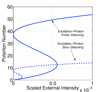
Figure 8: The average polariton number $\mathcal{N}$ vs. the scaled external field $|\tilde{F}|^{2}$, for the external field-polariton detuning of $\bar{\delta}=10^{-3}\ eV$, and with $k=10^{-6}\ \AA^{-1}$. The full line is at zero atom-photon detuning, $E_{C}(k)-E_{A}=0$, and the dashed line is for the case of finite detuning with $E_{C}(k)-E_{A}=-10^{-5}\ eV$.

VI Conclusions

The present paper is opened by introducing polaritons as natural excitations in a lattice of cold atoms strongly coupled to a nanophotonic waveguide, where a tapered nanofiber is used as a prototype system. Afterward we exploited a bosonization procedure that end in interacting polaritons by converting spin-half operators into combinations of boson ones with terms that result in polariton interactions. The kinematic polariton-polariton interaction is introduced as a significant mechanism for different nonlinear processes. The regime where polaritons behave as a dilute boson gas is presented, which is a step toward the possibility of achieving BEC of polaritons in such system. Emphasize is put on lower branch polaritons with long wavelengths that behave as quasi-particles with effective mass and finite zero energy. The coherent mixing of dispersion-less excitations and confined photons of parabolic dispersion leads to the above features of polaritons. The excitation-photon detuning is presented as a tool for controlling the kinematic polariton-polariton interaction strength.

The polariton-polariton scattering, due to the kinematic interaction, is for the polariton excitation part that modeled in the center of mass frame as a scattering of a polariton with a reduced mass from a potential that results of the other polariton, and which appears as a defect in the lattice. The polariton excitation part is completely backward scattered, and we concluded that the polariton backward scattering have reflection amplitude as their excitation amplitude, and the polariton forward scattering have transmission amplitude as their photonic amplitude. Significant exception appeared for large negative detuning, as here lower branch polaritons of long wave lengths are much more photonic than excitation and they are weakly interact via the kinematic interactions. Polaritons in this regime can be treated as interacting photons, where the issue of superfluidity of photons is proposed for such a system.

Different optical nonlinear processes are treated and presented as a tool for observing physical properties of the system. Here the finite life time of the fiber photons and of the excited atoms are included and external source fields contained. In the mean field theory we derived equations of motion for the polariton amplitudes and solved for the steady state case. The pump-probe experiment is introduced, where the weak probe spectrum calculated under the existence of fixed strong pump. The blue shift in the probe spectrum found to be proportional to the kinematic interaction strength. Furthermore, for identical counter propagating pump fields, we derived the steady state average number of photons for various parameters. In this case we extracted the atom-atom correlation of two separated atoms in the lattice that indicates possible significant long range interaction mediated by the cavity photons. For finite external pump-polariton detuning we got optical bistability behavior in the average number of polaritons as a function of the external pump intensity.

The above scattering results are directly adopted in the appendix for the scattering of polaritons from an impurity atom of different kind than the lattice atoms. The language of polaritons is shown to provide direct conclusions concerning the scattering problem, and more useful cases can be engineered. The scattering amplitude can be easily changed by controlling the impurity level relative to the lattice atoms in using external fields. The results of the present paper can be adapted for any set-up of one dimensional optically active materials that are strongly coupled to one dimensional propagating photons.

The author gratefully acknowledges helpful and fruitful discussions with Thomas Pohl.

Appendix A Polariton Scattering from an Atom Impurity in the Lattice

The appearance of defects in the atomic lattice is unavoidable in real experiments. In the present appendix we discuss the scattering of a polariton from an impurity atom of different type in the lattice that is localized in the origin, as seen in figure (9). The defect Hamiltonian is given by $H_{d}=\bar{E}\ B_{0}^{\dagger}B_{0}$, where $\bar{E}=E_{d}-E_{A}$, with $E_{d}$ is the impurity atom transition energy. Using the previous results for the scattering of small wave number polaritons with parabolic dispersion, one get the square scattering amplitude

$$|f(k)|^{2}=\frac{\frac{\bar{E}^{2}}{\Lambda^{2}}\left(\frac{\pi^{2}}{2ka}\right)^{2}|X_{k}^{-}|^{4}}{1+\frac{\bar{E}^{2}}{\Lambda^{2}}\left(\frac{\pi^{2}}{2ka}\right)^{2}|X_{k}^{-}|^{4}}.$$ (55)

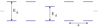
Figure 9: The atomic lattice of lattice constant $a$ with localized impurity of different transition energy $E_{d}$.

We present the results for the previous numbers. First we plot the eigen-energies in figure (10.a) and the excitation and photon fractions in figure (10.b) for the two branches as a function of the excitation-photon detuning, $E_{C}(k)-E_{A}$, for fixed small wave number of $k\approx 10^{-6}\ \AA^{-1}$, which is much smaller than $k_{0}$. Around zero excitation-photon detuning the polariton is half excitation and half photon. For large negative detuning the lower branch becomes more photonic and the upper one more excitation, and for large positive detuning the opposite the lower branch becomes more excitation and the upper one more photonic. Note that the detuning need to be much smaller than the atomic transition for the rotating wave approximation to hold.

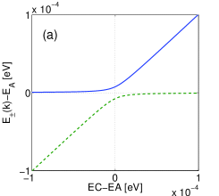
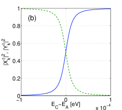
Figure 10: (a) The polariton relative energies $E_{\pm}(k)-E_{A}$ vs. the detuning $E_{C}(k)-E_{A}$ in the upper and lower branches by changing the photon energy, for $k=10^{-6}\ \AA^{-1}$. (b) The excitation and photon fractions in the two polariton branches vs. the detuning $E_{C}(k)-E_{A}$, for $k=10^{-6}\ \AA^{-1}$. In the upper branch the full line is for the photon fraction $|Y_{k}^{+}|^{2}$ and the dashed line for the excitation fraction $|X_{k}^{+}|^{2}$. In the lower branch the dashed line is for the photon fraction $|Y_{k}^{-}|^{2}$ and the full line for the excitation fraction $|X_{k}^{-}|^{2}$.

We plot in figure (11) the absolute square of the scattering amplitude, that is $|f(k)|^{2}$ as a function of the detuning $E_{C}(k)-E_{A}$ for small fixed wave number of $k\approx 10^{-6}\ \AA^{-1}$, and for deep impurity with $E_{d}=0$. Things are drastically changed for large negative detuning, as now the lower branch around small wave numbers becomes more photonic and in the off-resonance case the scattering become finite and drops down with increasing the negative detuning.

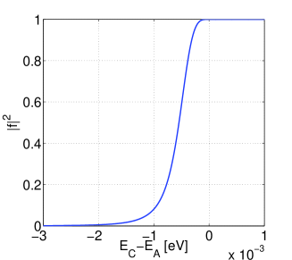
Figure 11: The absolute square of the scattering amplitude, $|f(k)|^{2}$ vs. the detuning $E_{C}(k)-E_{A}$, for $k=10^{-6}\ \AA^{-1}$, and with $E_{d}=0$.

The polariton for large negative detuning is weakly scattered in the limit of $\frac{\bar{E}}{\Lambda}\left(\frac{\pi^{2}}{2ka}\right)|X_{k}^{-}|^{2}\ll 1$, where the absolute value of the scattering amplitude is

$$|f(k)|\approx\frac{\bar{E}}{\Lambda}\left(\frac{\pi^{2}}{2ka}\right)|X_{k}^{-}|^{2}.$$ (56)

In the limit of large negative detuning the parabolic assumption holds and the contribution of the upper branch is negligible. Here the polaritons are weakly scattered from the vacancy.

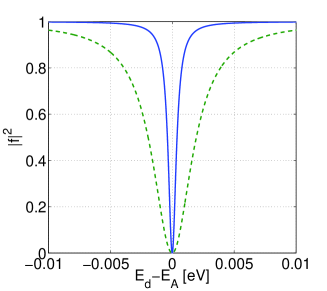
Figure 12: The absolute square of the scattering amplitude, $|f(k)|^{2}$ vs. the detuning $E_{d}-E_{A}$, for (full-line) $ka=5\times 10^{-3}$, and for (dashed-line) $ka=25\times 10^{-3}$.

As the defect potential is relatively a deep square well potential of depth $E_{A}$ and width $a$, the scattering is the same as that from a square barrier potential of height $E_{A}$ and width $a$. Namely, we have the known result that for deep potentials the appearance of bound states is immaterial as the probability to hit a resonance is very small. Hence the defect is repulsive potential where the polariton excitation part backward reflected, and only the polariton photon part have forward scattering or move through the defect without interaction.

For the case of $E_{C}(0)-E_{A}=0$, we have

$$|f(k)|^{2}=\frac{\frac{\bar{E}^{2}}{\Lambda^{2}}\left(\frac{\pi^{2}}{4ka}\right)^{2}}{1+\frac{\bar{E}^{2}}{\Lambda^{2}}\left(\frac{\pi^{2}}{4ka}\right)^{2}}.$$ (57)

In figure (12) we plot the square scattering amplitude, $|f|^{2}$, as a function of $\bar{E}$, for small wave number polaritons of $ka=5\times 10^{-3}$, and $ka=25\times 10^{-3}$, and in using the previous numbers where $\Lambda\approx 0.19\ eV$. It is clear that scattering resonance appears at $\bar{E}=0$ where the impurity become similar to the other lattice atoms. Complete scattering appears at large positive and negative $\bar{E}$. The resonance width is related on the wave number, where it is wide for large $k$ and narrow for small one. For the case of large positive and negative $\bar{E}$ the polariton transmission is $|Y_{0}|^{2}$ and the polariton reflection is $|X_{0}|^{2}$, which are $1/2$ for the case of $E_{C}(0)-E_{A}=0$.

The localization of two identical impurities at separation distance that is larger than $a$ gives rise to atomic mirror, as in the paper Chang , but here the results can be obtained directly in terms of polaritons. The scattering of polaritons from a defect in planar optical lattice in the Mott insulator phase with one atom per site has been studied in ZoubiE ; ZoubiRev .

References

- (1) F. Brennecke, T. Donner, S. Ritter, T. Bourdel, M. Kohl, and T. Esslinger, Nature 450, 268 (2007).
- (2) Y. Colombe, T. Steinmetz, G. Dubois, F. Linke, D. Hunger, and J. Reichel, Nature 450, 272 (2007).
- (3) E. Vetsch, D. Reitz, G. Sague, R. Schmidt, S. T. Dawkins, and A. Rauschenbeutel, Phys. Rev. Lett. 104, 203603 (2010).
- (4) A. Goban, K. S. Choi, D. J. Alton, D. Ding, C. Lacroute, M. Pototschnig, T. Thiele, N. P. Stern, and H. J. Kimble, Phys. Rev. Lett. 109, 033603 (2012).
- (5) H. J. Metcalf, and P. van der Straten, Laser Cooling and Trapping, (Springer, NY 1999).
- (6) D. Jaksch, C. Bruder, J. I. Cirac, C. W. Gardiner, and P. Zoller, Phys. Rev. Lett. 81, 3108 (1998).
- (7) M. Greiner, O. Mandel, T. Esslinger, T. W. Hansch, and I. Bloch, Nature 415, 39 (2002).
- (8) K. P. Nayak, P. N. Melentiev, M. Morinaga, F. L. Kien, V. I. Balykin, and K. Hakuta, Opt. Express 15, 5431 (2007).
- (9) K. P. Nayak, and K. Hakuta, New J. Phys. 10, 053003 (2008).
- (10) D. E. Chang, L. Jiang, A. V. Gorshkov, and H. J. Kimble, New J. Phys. 14, 063003 (2012).
- (11) D. E. Chang, J. I. Cirac, and H. J. Kimble, Phys. Rev. Lett. 110, 113606 (2013).
- (12) F. Dalfovo, S. Giorgini, L. P. Pitaevskii, and S. Stringari, Rev. Mod. Phys. 71, 463 (1999).
- (13) J. Kasprzak, M. Richard, S. Kundermann, A. Baas, P. Jeambrun, J. M. J. Keeling, F. M. Marchetti, M. H. Szymanska, R. Andre, J. L. Staehli, V. Savona, P. B. Littlewood, B. Deveaud, and L. S. Dang, Nature 443, 409 (2006).
- (14) R. Y. Chiao, Optics Commun., 179, 157 (2000).
- (15) J. Klaers, J. Schmitt, F. Vewinger, and M. Weitz, Nature 468, 545 (2010).
- (16) H. Zoubi, and H. Ritsch, New J. Phys. 12, 103014 (2010).
- (17) H. Zoubi, and H. Ritsch, Advances in Atomic, Molecular, and Optical Physics 62, 171, (Eds.: E. Arimondo, P. Berman, C. Lin), (Elsevier, 2013).
- (18) A. Kavokin, and G. Malpuech, Cavity Polaritons, Thin Films and Nanostruct., 32 (Elsevier, 2003).
- (19) H. Zoubi, and G. C. La Rocca, Phys. Rev. B 71, 235316 (2005).
- (20) A. Altland, and B. D. Simons, Condensed Matter Field Theory, (Cambridge, 2006).
- (21) T. Holstein, and H. Primakoff, Phys. Rev. 58, 1098 (1940).
- (22) V. M. Agranovich, and B. S. Toshich, Sov. Phys. JETP 26, 104 (1968).
- (23) P. W. Anderson, Concepts in Solids, (World Scientific, Singapore 1997).
- (24) H. Zoubi, and G. C. La Rocca, Phys. Rev. B 72, 125306 (2005).
- (25) R. Boyd, Nonlinear Optics, (Academic Press, San Diego, 2003).
- (26) H. Zoubi, Europhys. Lett. 100, 24002 (2012).
- (27) F. Warken, E. Vetsch, D. Meschede, M. Sokolowski, and A. Rauschenbeutel, Optics Express 15, 11952 (2007).
- (28) J. Dalibard, Proceedings of the International School of Physics “Enrico Fermi”, Course CXL: Bose-Einstein condensation in gases, Eds.: M. Inguscio, S. Stringari, C. Wieman, (IOS Press, Amsterdam, 1998).
- (29) L. P. Kadanoff, and G. Baym, Quantum statistical mechanics, (Benjamin-Cumming, Massachusetts, 1962).
- (30) R. G. Newton, Scattering Theory of Waves and Particles, (Springer, NY 1982).
- (31) H. Zoubi, and H. Ritsch, New J. Phys. 10, 023001 (2008).