Hamiltonian Theory of Anisotropic Fractional Quantum Hall States

Abstract

Rotationally invariant fractional quantum Hall (FQH) states have long been understood in terms of composite bosons or composite fermions. Recent investigations of both incompressible and compressible states in highly tilted fields, which renders them anisotropic, have revealed puzzling features which have so far defied quantitative explanation. The author’s work with R. Shankar in constructing and analyzing an operator-based theory in the rotationally invariant FQHE is generalized here to the anisotropic case. We compute the effective anisotropies of many principal fraction states in the lowest and the first Landau levels and find good agreement with previous theoretical results. We compare the effective anisotropy in a model potential with finite sample thickness and find good agreement with experimental results.

Our understanding of rotationally invariant FQH statesQH-reviews ; laugh is based on highly accurate variational wavefunctionslaugh ; jain , which rely on the idea of particle-flux composites. For fractions of the form $\nu=\frac{1}{2s+1}$ ($s$ integer) the Laughlin wavefunctionslaugh can be understood as ground states of composite bosonszhk (electrons carrying $2p+1$ units of statistical flux). A unified way to understand all principal fractions of the form $\frac{p}{2ps+1}$ is the composite fermion (CF) picture of Jainjain , in which the CF is a composite of an electron and $2s$ quanta of statistical flux. The CFs see an effective field just right to fill $p$ CF-Landau levels (CFLLs), thus naturally forming an incompressible state. CFs can be realized in a field theoretic form by Chern-Simons theorylopez-fradkin , which has had many successes, notably in the half-filled Landau levelHLR where the CFs form a Fermi sea.

Most experimental systems are not rotationally invariant. When the band mass tensor is isotropic and the magnetic length is much larger than the lattice spacing, rotational invariance is a good approximation. Tilting the sample while keeping the filling fixed has many effects, among which is an induced anisotropy of the band mass tensorKamburov-zero-B . Recently, anisotropic transport has been observed in strongly correlated states in the quantum Hall regimegokmen ; xia-73 ; Kamburov1 under strong tilted fields. It is found that the CF anisotropy is considerably smaller than the electronic oneKamburov1 , and at $7/3$, a peculiar low-temperaturexia-73 state with quantized Hall resistance, but highly anisotropic longitudinal resistance ($R_{yy}$ vanishing, but $R_{xx}$ seemingly finite) is seen. Taking steps towards understanding such states quantitatively will be the focus of this paper. Our approach will also apply to anisotropic cousins of the recently discovered FQH-like states in Chern bandschern and two-dimensional time-reversal-invariant topological insulators (2DTIs)2dti ; 2dti-numerics .

HaldaneHaldane-geo noted recently that there is an intrinsic geometry to the FQH regime. Start with an anisotropic band Hamiltonian in a uniform perpendicular ${\mathbf{B}}$ field

$$H_{0}=\frac{1}{2m}\bigg{(}\frac{\Pi_{ex}^{2}}{\alpha^{2}}+\Pi_{ey}^{2}\alpha^{2}\bigg{)}$$ (1)

where the subscript $e$ reminds us that the coordinate ${\mathbf{r}}_{e}=x_{e}{\hat{i}}+y_{e}{\hat{j}}$ and mechanical momentum ${\mathbf{\Pi}}_{e}$ are electronic operators, and $\alpha$ is our electronic anisotropy parameter. The cyclotron frequency is $\omega_{c}=\frac{eB}{m}$ and the magnetic length is $l=\sqrt{\frac{h}{eB}}$. The electronic Hilbert space can be decomposed into two “cyclotron” coordinates ($a,b=x,y$ and $\epsilon_{ab}$ is the two-dimensional antisymmetric symbol) $\eta_{ea}=-l^{2}\epsilon_{ab}\Pi_{b}$ and two guiding center coordinates $R_{ea}=r_{ea}-\eta_{ea}$. These two sets have the commutation relations $[\eta_{ex},\eta_{ey}]=il^{2}=-[R_{ex},R_{ey}]$, and $[\eta_{ea},R_{eb}]=0$.

Letting $i$ index particle number, the density operator in first quantization is

$$\rho_{e}({\mathbf{q}})=\sum\limits_{i}e^{i{\mathbf{q}}\cdot{\mathbf{\eta}}_{ei}}e^{i{\mathbf{q}}\cdot{\mathbf{R}}_{ei}}$$ (2)

When projected to the $n^{th}$ LL, this density becomes

$$e^{-|z|^{2}/2}L_{n}(|z|^{2})\sum\limits_{i}e^{i{\mathbf{q}}\cdot{\mathbf{R}}_{ei}}=e^{-|z|^{2}/2}L_{n}(|z|^{2}){\bar{\rho}}_{e}({\mathbf{q}})$$ (3)

where $z=i\frac{l}{\sqrt{2}}\big{(}\frac{q_{x}}{\alpha}+iq_{y}\alpha\big{)}$, and $L_{n}$ is the $n^{th}$ Laguerre polynomial. Here the projected guiding center density ${\bar{\rho}}_{e}({\mathbf{q}})$ is also the operator generating magnetic translations in a given LL, and obeys the GMP algebra (named in honor of Girvin, MacDonald, and PlatzmanGMP )

$$[{\bar{\rho}}_{e}({\mathbf{q}}),{\bar{\rho}}_{e}({\mathbf{q}}^{\prime})]=2i\sin\bigg{(}i\epsilon_{ab}q_{a}q^{\prime}_{b}\frac{l^{2}}{2}\bigg{)}{\bar{\rho}}_{e}({\mathbf{q}}+{\mathbf{q}}^{\prime})$$ (4)

Since the kinetic energy is degenerate, the Hamiltonian when projected to the $n^{th}$ Landau level is

$$\bar{H}={1\over 2}\int\frac{d^{2}q}{(2\pi)^{2}}{\tilde{v}}(q):{\bar{\rho}}_{e}({\mathbf{q}}){\bar{\rho}}_{e}(-{\mathbf{q}}):$$ (5)

where the effective electron interaction is ${\tilde{v}}({\mathbf{q}})=v(q)e^{-|z|^{2}/2}L_{n}(|z|^{2})$.

Haldane pointed outHaldane-geo that the effective anisotropy of the FQH state would be a compromise between the anisotropies of the band mass and the interaction anisotropy (here assumed to be 1).

Very early work on anisotropic statesearly-aniso focussed on spontaneous breaking of rotational symmetry. An application of Chern-Simons theory predicted that the electronic and CF anisotropies should be identicalbalagurov at $\nu={1\over 2}$, in contradiction with experimentKamburov1 . More recent theoretical work on anisotropic FQH states has been mainly numerical, involving comparing ground states obtained by exact diagonalization with model wavefunctionsModel-wfs ; variational-Haldane ; numerics . The special case of a gaussian interaction in the LLL can be analyzed exactlykunyang , but unfortunately this cannot be extended to realistic interactions, or other Landau levels.

In this paper we analytically compute ${\alpha^{CF}}$ as a function of $\alpha$ given the Landau level one is projecting to, the fraction, and the form of the interelectron interaction. We will test this approach by comparing to the numerical resultsvariational-Haldane , and find good agreement. We will compare the effects of band mass anisotropy in the zeroth and the first Landau levels for the Coulomb interaction, and consider the effects of finite sample thickness. Finally, we will compare to experimental results on the relation between ${\alpha^{CF}}$ and $\alpha$ for the half-filled Landau levelKamburov1 , and see agreement for reasonable sample thickness.

The method we use is a generalization of the approach developed by R. Shankar and the author more than a decade agoprl-us ; rmp-us . This approach starts with a rewriting of the electronic Hamiltonian in a given Landau level in an enlarged Hilbert space spanned by operators obeying CF commutation relations. The spurious degrees of freedom have to ultimately be projected out in a suitable mannerconserving ; resp-fns-us . While approximate, this approach allows us to compute various quantities which are difficult, if not impossible, in conventional wavefunction or exact diagonalization treatments, such as response functionsresp-fns-us , the effects of nonzero temperaturefiniteTus , or disorderdisorder-us .

In a particular LL, the electronic degrees of freedom are the guiding centers $R_{ex},\ R_{ey}$. To make a complete fermionic Hilbert space we add by hand two pseudovortex degrees of freedom per electron $R_{vx},\ R_{vy}$, so called because they have the commutation relations of a double vortex $[R_{vx},R_{vy}]=\frac{il^{2}}{2\nu}=\frac{il^{2}}{c^{2}}$ which defines $c=\sqrt{2\nu}$ for the case of two flux quanta “attached”. Since they are unphysical degrees of freedom, they commute with ${\mathbf{R}}_{e}$: $[R_{ea},R_{vb}]=0$. Now we re-express ${\mathbf{R}}_{e},\ {\mathbf{R}}_{v}$ in terms of CF coordinates and velocities. Note that the CF degrees of freedom have no subscripts, and obey the commutation relations $[r_{xi},r_{yi}]=0$, $[r_{ai},\Pi_{bi}]=i\delta_{ab}$, and most importantly, $[\Pi_{xi},\Pi_{yi}]=\frac{i}{(l^{*})^{2}}=\frac{i(1-c^{2})}{l^{2}}$. The last relation shows that the CF’s move in a reduced field. Define the CF-cyclotron variables by $\eta_{a}=-(l^{*})^{2}\epsilon_{ab}\Pi_{b}$, and the CF guiding center variables by $R_{a}=r_{a}-\eta_{a}$. In the isotropic FQH regime, we made the identification

$${\mathbf{R}}_{e}={\mathbf{R}}+c{\mathbf{\eta}}\ \ \ \ \ \ \ {\mathbf{R}}_{v}={\mathbf{R}}+{\mathbf{\eta}}/c$$ (6)

We expressed the projected density ${\bar{\rho}}({\mathbf{q}})$ in terms of CF variables and proceeded to find a Hartree-Fock ground state (CFHF for short). For $\nu=\frac{p}{2p+1}$ the HF ground state was just $p$ filled CF-Landau levels (CFLLs).

The CF-substitution for the anisotropic problem is similar. We leave the expression for ${\mathbf{R}}_{v}$ unchanged but make the expression for ${\mathbf{R}}_{e}$ anisotropic:

$$R_{ex}=(R_{x}+c\eta_{x})/{\alpha^{CF}}:\ \ \ \ R_{ey}=(R_{y}+c\eta_{y}){\alpha^{CF}}$$ (7)

Note that the ${\mathbf{R}}_{e}$ and thus the Hamiltonian still commute with ${\mathbf{R}}_{v}$, and the constraint structure is unaltered. Now we can express the Hamiltonian in terms of CF variables and proceed as in the isotropic case.

With an eye to generalizing this approach to anisotropic states in Chern bands and 2DTIsTI-us we will find it convenient to use crystal momenta in a Brillouin Zone in the given Landau level. For a principal fraction $\frac{p}{2p+1}$ it is now straightforward to rescale the momenta ($Q_{x}=q_{x}/\alpha^{CF},\ Q_{y}=q_{y}\alpha^{CF}$), choose a unit cell penetrated by an integer number of effective flux quanta ($a(2p+1)$ in the $x$-direction and $a$ in the $y$-direction, where $a^{2}=2\pi l^{2}$), and thus define a single-CF Brillouin Zone (details can be found in ref. TI-us ) with canonical fermion operators $d^{\dagger}_{n{\mathbf{K}}},\ d_{n{\mathbf{K}}}$, in terms of which the electron guiding center density and Hamiltonian are

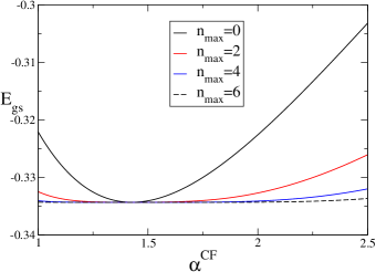
Figure 1: The CFHF energy per particle at ${1\over 3}$ in the LLL for $\alpha=2$ versus ${\alpha^{CF}}$ for different numbers of CFLLs kept ($n_{max}$). The interaction is pure Coulomb.

$${\bar{\rho}}_{e}({\mathbf{Q}})= \sum\limits_{{\mathbf{K}}\in BZ,n^{\prime},n}\rho_{n^{\prime}n}({\mathbf{Q}})e^{i\Phi({\mathbf{Q}},{\mathbf{K}})}d^{\dagger}_{n^{\prime}[{\mathbf{K}}+{\mathbf{Q}}]}d_{n{\mathbf{K}}}$$ (8)

$$H= \frac{1}{2L^{2}}\sum\limits_{{\mathbf{Q}}}{\tilde{v}}({\mathbf{Q}}):{\bar{\rho}}_{e}({\mathbf{Q}}){\bar{\rho}}_{e}(-{\mathbf{Q}}):$$ (9)

Here $[{\mathbf{K}}+{\mathbf{Q}}]$ belongs to the BZ, and is defined by ${\mathbf{K}}+{\mathbf{Q}}=[{\mathbf{K}}+{\mathbf{Q}}]+\frac{2\pi}{a}N_{y}({\mathbf{Q}},{\mathbf{K}})+\frac{2\pi}{a(2p+1)}N_{x}({\mathbf{Q}},{\mathbf{K}})$, and $\Phi({\mathbf{Q}},{\mathbf{K}})=\frac{2p+1}{a^{2}}\big{(}-(K_{x}+Q_{x})N_{y}({\mathbf{Q}},{\mathbf{K}})+\frac{Q_{x}}{2\pi}(K_{y}+\frac{Q_{y}}{2})\big{)}$.

To define the matrix elements $\rho_{mn}({\mathbf{Q}})$ compactly we need $Z=\frac{cl^{*}}{\sqrt{2}}(Q_{x}+iQ_{y})=|Z|e^{i\theta}$, in terms of which

$$\rho_{n^{\prime}n}({\mathbf{Q}})= (-1)^{min(n^{\prime},n)+n}\sqrt{\frac{min(n^{\prime},n)!}{max(n^{\prime},n)!}}e^{-|Z|^{2}/2}$$ (10)

$$L_{min(n^{\prime},n)}^{|n^{\prime}-n|}(|Z|^{2})|Z|^{|n^{\prime}-n|}e^{i(n^{\prime}-n)(\theta-\pi/2)}$$

Translationally invariant CFHF states for $\nu=\frac{p}{2p+1}$ correspond to averages

$$\langle d^{\dagger}_{m{\mathbf{K}}^{\prime}}d_{n{\mathbf{K}}}\rangle=\delta_{{\mathbf{K}},{\mathbf{K}}^{\prime}}\Delta_{mn}$$ (11)

where $\Delta_{mn}$ are independent of ${\mathbf{K}}$. The $\nu={1\over 2}$ state will be treated as the $p\to\infty$ limit.

Two important points need to be noted: (i) The CFHF energy is variational. The Hamiltonian commutes with all the ${\mathbf{R}}_{vi}$, so the exact ground state in the enlarged Hilbert space must be a direct product of the exact ground state in the ${\mathbf{R}}_{e}$ sector and an arbitrary state in the ${\mathbf{R}}_{v}$ sector. Since the Hamiltonian is independent of ${\mathbf{R}}_{v}$ the exact ground state energy in the enlarged space is the same as that in the electronic space. (ii) For incompressible fractions, every set of $\Delta_{mn}$ defines a Slater determinant state, so for fixed $\alpha,{\alpha^{CF}},\nu$ there is still a lot of freedom. For a given $\alpha,\ {\alpha^{CF}}$, we iterate the HF procedure till we have a self-consistent set of $\Delta_{mn}$.

These points are illustrated in Fig. 1, which shows the ground state energy per particle for ${1\over 3}$ at an electronic anisotropy of $\alpha=2$ as a function of the assumed CF anisotropy ${\alpha^{CF}}$. The different curves represent different numbers of CFLL’s kept in the variational calculation. All the results we present are for the Coulomb interaction $v(q)=2\pi e^{2}/\varepsilon q$ unless stated otherwise.

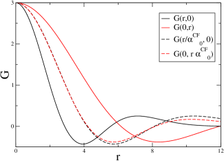
Figure 2: The one-body correlator in the $x$ and $y$-directions at $\nu=\frac{3}{7}$ in the LLL for $\alpha=2$. The solid lines are the unscaled correlators, while the dashed lines are the corresponding scaled correlators for $\alpha^{CF}_{0}=1.46$.

As can be seen, as $n_{max}$ increases the energy becomes extremely flat, i.e., nearly independent of ${\alpha^{CF}}$. This is because the full set of CFLLs at $\alpha^{CF}_{1}$ is related to the full set at $\alpha^{CF}_{2}$ by a unitary transformation of the form $e^{i\gamma\eta_{x}\eta_{y}/l^{2}}$. Thus, the ground state at any $\alpha$ can be written for any ${\alpha^{CF}}$, and the ground state energy is not useful in selecting the optimal ${\alpha^{CF}}$.

To find the optimal CF anisotropy ${\alpha^{CF}}$ we turn to the equal-time single-particle correlator $G(x,y)$ which is an implicit function of $\Delta_{mn}$. It is easily checked that $G(x,y)$ is (nearly) independent (for large but finite $n_{max}$) of ${\alpha^{CF}}$ in the same way that the $E_{gs}$ per particle is (see appendix).

Given a $\alpha$, we will define the optimal value of ${\alpha^{CF}_{0}}(\alpha)$ by demanding that $G(\frac{x}{{{\alpha^{CF}_{0}}}},y{{{\alpha^{CF}_{0}}}})$ be as close to isotropic as possible. Fig. 2 shows the unscaled correlators in the two directions $G(r,0)$ and $G(0,r)$ versus $r$, as well as the scaled versions with the optimal scaling ($\alpha^{CF}_{0}=1.46$) for $\nu=\frac{3}{7}$ in the LLL for the Coulomb interaction. As can be seen, one cannot make the correlators in the $x,\ y$ directions truly equal by a simple rescaling. The best that can be done is to arrange for the maxima and minima to be at the same location.

In this way we determine $\alpha^{CF}_{0}(\alpha)$, which depends on the interaction (Coulomb), the LL into which we have projected the electron density, and the principal fraction in question (represented by the integer $p$, where $\nu=\frac{p}{2p+1}$). As $p$ becomes larger $\alpha^{CF}_{0}$ saturates to a value we assume is the relevant one for $\nu={1\over 2}$. Fig. 3 shows the dependence for the LLL and the first Landau level (FLL).

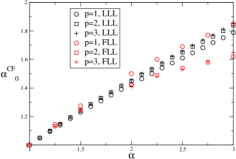
Figure 3: The optimal value of ${\alpha^{CF}}$ plotted as a function of $\alpha$ for the first few principal fractions in the LLL and the FLL. The size of the symbols roughly captures the uncertainty of estimating $\alpha^{CF}_{0}$ by trying to collapse $G(r/\alpha^{CF}_{0},0)$ and $G(0,r\alpha^{CF}_{0})$.

For $\nu={1\over 3}$ in the LLL, our result is close to that of Yang et alvariational-Haldane who estimate $\alpha^{CF}_{0}$ by finding the largest overlap of the exact ground state with an anisotropic Laughlin wave functionHaldane-geo . Their definition of the anisotropy is the square of ours. Looking Figure 3 of Yang et alvariational-Haldane and translating to our anisotropies, we see that at $\alpha=\sqrt{2}$ they get $\alpha^{CF}_{0}=\sqrt{1.37}=1.17$, while our result is $\alpha^{CF}_{0}=1.185$.

Another criterion for the optimal $\alpha^{CF}$ might be to determine when the state is closest to the correponding isotropic Jain statejain . One can compute the total occupation of the lowest $p$ CFLLs as a function of $\alpha^{CF}$ and find $\alpha^{CF}_{0}$ by maximizing it. Reassuringly, this criterion gives the same $\alpha^{CF}_{0}$ as does the collapse of $G(x\alpha^{CF}_{0},0)$ and $G(0,y\alpha^{CF}_{0})$ (see Appendix).

Finally, our results for the exactly solvable gaussian interaction in the LLL $v(q)=e^{-(\lambda ql)^{2}/2}$ agree perfectly (see Appendix) with the expression of Kun Yangkunyang $\alpha^{CF}_{0}=\big{(}\frac{\alpha^{2}+\lambda^{2}}{\alpha^{-2}+\lambda^{2}}\big{)}^{1/4}$ for all fractions. These checks show that CFHF captures the essential physics of the anisotropic FQHE.

It is interesting to see that in the LLL, ${1\over 3}$ has a higher value of $\alpha^{CF}_{0}$ for a given $\alpha$ than other principal fractions, while the reverse is true in the FLL. For a given $\alpha$, as $p$ increases $\alpha^{CF}_{0}$ saturates rapidly. Experimental measurements of the CF anisotropy have been carried out at $\nu={1\over 2}$ by Kamburov et al Kamburov1 . Noting that their definition of the anisotropy is the square of ours, they find at $\alpha=\sqrt{3}$ a CF-anisotropy of $\alpha^{CF}_{0}=\sqrt{1.3}\simeq 1.15$Kamburov1 .

For the Coulomb interaction, for $\alpha=\sqrt{2}$ and large $p=3,4,5$, we find a $\alpha^{CF}_{0}$ of about $1.34$, which is high compared to the experiment. To understand the discrepancy, we turn to a cartoon model of the finite thickness of the 2DEG, and its effects on $\alpha^{CF}_{0}$. We will assume that the Coulomb potential has been modified to

$$v_{\lambda}(q)=\frac{2\pi e^{2}}{\varepsilon q}e^{-(\lambda ql)^{2}/2}$$ (12)

where $\lambda$ is a dimensionless parameter representing the thickness of the 2DEG. A reasonable value of $\lambda$ for an experimental sample would be of order 1. Fig. 4 shows the variation of $\alpha^{CF}_{0}$ with $\lambda$ for $\alpha=\sqrt{3}$.

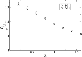
Figure 4: The variation of $\alpha^{CF}_{0}$ with the parameter $\lambda$ modelling sample thickness ina Coulomb interaction for ${1\over 3}$ and $\frac{5}{11}$. The latter fraction is a proxy for the $\nu={1\over 2}$ state.

As expected, $\alpha^{CF}_{0}$ decreases with thickness, and reasonable values of $\lambda\simeq 1$ can give rise to the experimentally measured CF anisotropyKamburov1 .

In summary, we have generalized the Hamiltonian approach for the FQH regime derived by R. Shankar and the present authorprl-us ; rmp-us to the case of systems with electronic anisotropy. This approach applies to any Landau level, arbitrary interactions, and any principal fraction. While the exact spectrum of the Hamiltonian in the enlarged Hilbert space is identical to that of the electronic Hamiltonian, the usefulness of the approach lies in approximations such as Composite Fermion Hartree Fock. We find that the equal time single-CF correlator provides a good way to estimate the CF anisotropy $\alpha^{CF}_{0}$ for any given $\alpha$. Our results are in good to excellent agreement with previous onesvariational-Haldane ; kunyang . For principal fractions labelled by $p$, where $\nu=\frac{p}{2p+1}$, $\alpha^{CF}_{0}$ increases with $p$ in the LLL, but decreases with $p$ in the first Landau level. In both cases $\alpha^{CF}_{0}$ saturates rapidly with increasing $p$.

We have also investigated the effect of finite sample thickness by using a model potential. We find that $\alpha^{CF}_{0}$ decreases with sample thickness, and reasonable values of the thickness parameter give CF anisotropies in agreement with experimentKamburov1 .

There are many directions in which this approach can be extended. The conserving approximationresp-fns-us can be used to compute magnetoexciton dispersions and response functions. This will help us identify potential instabilities of anisotropic FQH states. Recall that we restricted our variational search to translation invariant states. It is possible that stripe states formed of CFs (natural in the presence of anisotropy and CFLL mixing) are lower in energy than translationally invariant ones. Such states, when suitably dressed by quantum/thermal fluctuations and disorder may help us understand the peculiar behavior of the longitudinal resistivities at $\nu=\frac{7}{3}$xia-73 , which is currently not understood (see, however, mulligan ).

A second direction in which this approach could be useful is in analyzing anisotropic strongly correlated states in topological (Chern) bandschern and two-dimensional time-reversal invariant topological insulators (2DTIs)2dti . There has been much recent excitement with the numerical discovery of FQH states in such systems2dti-numerics . For topological bands and 2DTIs with conserved $S_{z}$, R. Shankar and the author have shownTI-us that the interacting Hamiltonian can once again be analyzed in CF language. The author intends to investigate these and other issues in the near future.

The author is grateful to the Aspen Center for Physics (NSF 1066293) for its hospitality while this work was conceived. He would also like to thank J. K. Jain, R. Shankar, and H. A. Fertig for illuminating conversations, and is grateful for partial support from NSF-PHY 0970069 (GM), and the US-Israel Binational Science Foundation-2012120.

I Appendix A

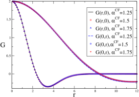
Figure 5: The unscaled correlators $G(r,0)$ and $G(0,r)$ for $\alpha=3$ and $\nu=\frac{2}{5}$ for different values of $\alpha^{CF}$. The interaction is Coulomb.

In order to use the equal-time correlator to extract the effective CF anisotropy $\alpha^{CF}_{0}$, we need to be sure that the correlator is independent of the nominal value of $\alpha^{CF}$. Fig. 5 shows the $\alpha^{CF}$-independence of the unscaled correlators for $\nu=\frac{2}{5}$. The electronic anisotropy is $\alpha=3$, the nominal values of $\alpha^{CF}_{0}$ run from 1.25 to 1.75, and 9 CFLLs are being kept. This holds true of arbitrary fractions and any $\alpha$.

A different way to extract the optimal CF anisotropy is to ask at what $\alpha^{CF}$ the ground state is closest to the corresponding Jain state of $p$ filled CFLLsjain . Our state is in an enlarged Hilbert space, so the best we can do is to compare the combined occupation of the lowest $p$ CFLLs to $p$. Figs. 6 and 7 show the normalized occupation $\frac{1}{p}\sum\limits_{0}^{p-1}\Delta_{nn}$ versus $\alpha^{CF}$ in the LLL and FLL.

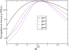
Figure 6: The normalized occupation of the lowest $p$ CFLLs versus $\alpha^{CF}$ for $\alpha=3$ in the LLL for the Coulomb interaction.

Comparing to Fig. 3, for each fraction, the value of $\alpha^{CF}$ at which the normalized occupation is maximum is almost identical to the $\alpha^{CF}_{0}$ obtained from the collapse of $G(r/\alpha^{CF}_{0},0)$ and $G(0,r\alpha^{CF}_{0})$. This makes sense because the Jain state with the lowest $p$ CFLLs filled is isotropic.

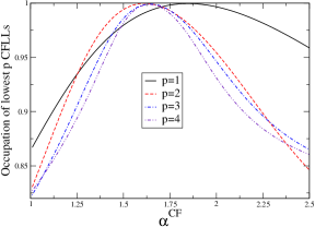
Figure 7: The normalized occupation of the lowest $p$ CFLLs versus $\alpha^{CF}$ in the first Landau level for the Coulomb interaction.

For the special case of a gaussian interaction ($v(q)=e^{-(\lambda ql)^{2}/2}$) in the LLL, $\alpha^{CF}_{0}$ can be exactly expressed in terms of $\alpha$ and the length scale $\lambda$ of the interaction askunyang

$$\alpha^{CF}_{0}=\big{(}\frac{\alpha^{2}+\lambda^{2}}{\alpha^{-2}+\lambda^{2}}\big{)}^{1/4}$$ (13)

In Fig. 8 we show the unscaled and scaled correlators in our approach for $\frac{1}{3}$ and $\frac{3}{7}$, where the correlators have been scaled with the exact value of $\alpha^{CF}_{0}$. The collapse of the correlator is nearly perfect.

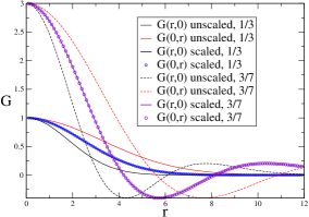
Figure 8: The unscaled and scaled correlators for a pure gaussian interaction at $\alpha=3,\ \lambda=2$, for $\nu=\frac{1}{3}$ and $\frac{3}{7}$ in the LLL.

References

- (1) The Quantum Hall Effect, R. Prange and S. M. Girvin, Editors, Springer-Verlag, New York 1990. Perspectives in Quantum Hall Effects, S. Das Sarma and A. Pinczuk, Editors, John Wiley, New York, 1997.
- (2) R. B. Laughlin, Phys. Rev. Lett. 50, 1395 (1983).
- (3) S.-C. Zhang, H. Hansson, and S. A. Kivelson, Phys. Rev. Lett. 62, 82 (1989).
- (4) J. K. Jain, Phys. Rev. Lett. bf 63, 199 (1989); Phys. Rev. B41, 7653 (1990); Science 266, 1199 (1994).
- (5) A. Lopez and E. Fradkin, Phys. Rev. B44, 5246 (1991); Phys. Rev. Lett. 69, 2126 (1992); Phys. Rev. B47, 7080 (1993).
- (6) B. I. Halperin, P. A. Lee, and N. Read, Phys. Rev. B47, 7312 (1993).
- (7) D. kamburov, M. Shayegan, R. Winkler, L. N. Pfeiffer, K. W. West and K. W. Baldwin, Phys. Rev. B86, 241302(R) (2012); D. Kamburov, M. A. Mueed, M. Shayegan, L. N. Pfeiffer, K. W. West, K. W. Baldwin, J. J. D. Lee, and R. Winkler, Phys. Rev. B88, 125435 (2013).
- (8) M. P. Lilly, K. B. Cooper, J. P. Eisenstein, L. N. Pfeiffer, and K. W. West, Phys. Rev. Lett. 82, 394 (1999); R. R. Du, D. C. Tsui, H. L. Stormer, L. N. Pfeiffer, and K. W. West, Solid State Commun. 109, 389 (1999).
- (9) T. Gokmen, M. Padmanabhan, M. Shayegan, Nature Phys. 6, 621 (2010).
- (10) J. Xia, J. P. eisenstein, L. N. Pfeiffer, and K. W. West, Nature Phys. 7, 845 (2011).
- (11) D. Kamburov, Y. Liu, M. Shayegan, L. N. Pfeiffer, K. W. West, and K. W. Baldwin, Phys. Rev. Lett. 110, 206801 (2013).
- (12) F. D. M. Haldane, Phys. Rev. Lett. 61, 2015, (1988); G. E. Volovik, Sov. Phys. JETP 67, 1804 (1988).
- (13) S. Murakami, N. Nagaosa, and S.-C. Zhang, Phys. Rev. Lett. 93, 156804 (2004); C. L .Kane and E. J. Mele, Phys. Rev. Lett. 95, 146802 (2005); C. L. Kane and E. J. Mele, Phys. Rev. Lett. 95, 226801 (2005); B. A. Bernevig and S.-C. Zhang, Phys. Rev. Lett. 96, 106802 (2006).
- (14) T. Neupert, L. Santos, C. Chamon, C. Mudry, Phys. Rev. Lett. 106, 236804 (2011); D. N. Sheng, Z. Gu, K. Sun, L. Sheng, Nature Communications 2, 389 (2011); N. Regnault and A. Bernevig, Phys. Rev. X1, 021014 (2011).
- (15) F. D. M. Haldane, Phys. Rev. Lett. 107, 116801 (2011).
- (16) S. M. Girvin, A. H. MacDonald, and P. M. Platzman, Phys. Rev. B33, 2481 (1986).
- (17) K. Musaelian and R. Joynt, J. Phys. Condens. Matter 8, L105 (1996); O. Ciftja and C. Wexler, Phys. Rev. B65, 045306 (2001); M. M. Fogler, Europhys. Lett. 66, 572 (2004).
- (18) D. B. Balagurov and Yu. E. Lozovik, Phys. Rev. B62, 1481 (2000).
- (19) R.-Z. Qiu, F. D. M. Haldane, X. Wan, Kun Yang, and S. Yi, Phys. Rev. B85, 115308 (2012).
- (20) Bo Yang, Z. Papic, E. H. Rezayi, R. N. Bhatt, and F. D. M. Haldane, Phys. Rev. B85, 165318 (2012).
- (21) H. Wang, R. Narayanan, X. Wan, and Fuchun Zhang, Phys. Rev. B86, 035112 (2012).
- (22) Kun Yang, arXiv:1309.2830 (2013).
- (23) R. Shankar and G. Murthy, Phys. Rev. Lett. 79, 4437 (1997).
- (24) G. Murthy and R. Shankar, Rev. Mod. Phys. 75, 1101 (2003).
- (25) G. Baym and L. P. Kadanoff, Phys. Rev.124, 287 (1961): N. Read, Phys. Rev. B58, 16262 (1998).
- (26) G. Murthy, Phys. Rev. B64, 195310 (2001).
- (27) G. Murthy, J. Phys. Condes. Matter 12, 10543 (2000).
- (28) G. Murthy and R. Shankar, Phys. Rev. B76, 075341 (2007); G. Murthy, Phys. Rev. Lett. 103, 206802 (2009).
- (29) G. Murthy and R. Shankar, Phys. Rev. B86, 195146 (2012).
- (30) See supplementary material.
- (31) M. Mulligan, C. Nayak, and S. Kachru, Phys. Rev. B82, 085102 (2010).