Toward a hybrid dynamo model for the Milky Way

Abstract

Context. Based on the rapidly increasing all-sky data of Faraday rotation measures and polarised synchrotron radiation, the Milky Way’s magnetic field is now modelled with an unprecedented level of detail and complexity.

Aims. We aim to complement this heuristic approach with a physically motivated, quantitative Galactic dynamo model – a model that moreover allows for the evolution of the system as a whole, instead of just solving the induction equation for a fixed static disc.

Methods. Building on the framework of mean-field magnetohydrodynamics and extending it to the realm of a hybrid evolution, we perform three-dimensional global simulations of the Galactic disc. To eliminate free parameters, closure coefficients embodying the mean-field dynamo are calibrated against resolved box simulations of supernova-driven interstellar turbulence.

Results. The emerging dynamo solutions comprise a mixture of the dominant axisymmetric S0 mode, with even parity, and a sub-dominant A0 mode, with odd parity. Notably, such a superposition of modes creates a strong localised vertical field on one side of the Galactic disc. We moreover find significant radial pitch angles, which decay with radius – explained by flaring of the disc. In accordance with previous work, magnetic instabilities appear to be restricted to the less-stirred outer Galactic disc. Their main effect is to create strong fields at large radii such that the radial scale length of the magnetic field increases from $4\,\rm kpc$ (for the case of a mean-field dynamo alone) to about $10\,\rm kpc$ in the hybrid models – the latter being in much better agreement with observations.

Conclusions. There remain aspects (e.g., spiral arms, X-shaped halo fields, fluctuating fields) that are not captured by the current model and that will require further development towards a fully dynamical evolution. Nevertheless, the work presented demonstrates that a hybrid modelling of the Galactic dynamo is feasible and can serve as a foundation for future efforts.

1 Introduction

The Galactic magnetic field (GMF) can now be modelled with an ever increasing level of detail (see e.g. Brown et al., 2007; Jaffe et al., 2010, 2011; Fauvet et al., 2011; Van Eck et al., 2011; Jansson & Farrar, 2012a, b; Mao et al., 2012). This becomes possible with the availability of all-sky data of Faraday rotation measures (Oppermann et al., 2012) and polarised synchrotron emission obtained by space missions like WMAP or Planck (see Fauvet et al., 2012). The typical approach utilises $\chi^{2}$ minimisation for fitting a large number of free parameters.

Theoretical models for the GMF are largely heuristic and guided by existing knowledge, e.g. derived from external galaxies. Modelling assumptions such as the winding angle of the spiral arms and its variation with radius (and near reversals) remain under debate (see e.g. discussion in Brown, 2010). From a theoretician’s point of view, these models still provide a convenient link to observations and can serve as a benchmark for dynamo models in the framework of mean-field MHD (Beck et al., 1996; Brandenburg et al., 2012b). Despite the success of the heuristic description, a thorough understanding of the underlying field amplification mechanism appears desirable.

Different flavors of mean field models have been studied for typical galaxies, yet under many simplifying assumptions. As for models specifically designed for the GMF, the most prominent difference of the Milky Way magnetic field in comparison with external galaxies shows up in the observationally now well supported (see e.g. discussion in Kronberg & Newton-McGee, 2011) reversal of the mean magnetic field in the radial direction – which has never yet been observed in other galaxies. Mean field models allow such field reversals in principle, depending on the seeding of the dynamo process (Moss & Sokoloff, 2012). Alternative explanations include oscillating solutions due to a vertical dependence of differential rotation (Ferrière & Schmitt, 2000) or, as proposed in this paper, a vertical undulation of the Galactic midplane combined with an antisymmetric vertical parity of the disc field, leading to apparent reversals. Yet another possibility, investigated here for the first time, is the mode interface between the dynamo-dominated inner region and the instability-dominated outer region of the Galaxy.

A further peculiarity of the GMF is the rather small pitch angle (of $\,\hbox{\lower 1.50696pt\hbox{$\sim$}\hbox to0.0pt{\hss\raise 1.50696pt\hbox{$<$}}}\,10\degr$) compared to many other galaxies with similar strong differential rotation and pitch angles up to $\sim 45\degr$ like, e.g., observed in M94 and M33 (Chyży & Buta, 2008; Tabatabaei et al., 2008). This dominance of the azimuthal field appears to be in better agreement with mean field models than with the large pitch angles observed in external galaxies. The magnetic field of mean-field dynamos is usually a stationary axisymmetric quadrupole. But for some cases like weak differential rotation or including the halo in the dynamo process, dipolar and/or oscillatory solutions may occur (Elstner et al., 1992; Brandenburg et al., 1992; Moss et al., 2010). The flaring of the Galactic disc was usually ignored in the modelling but has been considered in some recent publications (Moss et al., 2013; Chamandy et al., 2013a, b). This is despite the fact that observations seem to favour a non-flaring disc, at least in HII– see Lazio & Cordes (1998), and discussion in Moss et al. (2013). Our own model is guided by more recent observations (Kalberla & Dedes, 2008) of the HI distribution, which is indeed found to be flared.

A notable exception to dynamo models with constant scale height is the work by Poezd, Shukurov, & Sokoloff (1993), who assume a flared gas distribution and apply mean field models in the thin disc approximation to the Milky Way, relying on an observed rotation curve, and estimates for disc height, turbulent velocity, correlation length and gas density. They derive radial profiles of the final magnetic field for regular and chaotic seed fields with $\alpha$ quenching due to magnetic helicity. The maximum field strength of the regular field appeared at about $6\,\rm kpc$. For strong enough seed field (0.001 to $0.1\,\mu\rm G$) they found reversals.

While such models have provided us with a wealth of qualitative understanding of the expected mode structure appearing in $\alpha\Omega$ type disc dynamos, they lack a rigorous foundation for the actual amplitude and spatial distribution of the imposed mean-field effects. Recently, a quantitative measurement of the transport coefficients has become possible by employing the so-called test-field (TF) method (Schrinner et al., 2005) to realistic local simulations of interstellar turbulence (Gressel et al., 2008b). This also includes the determination of quenching functions (Gressel, Bendre, & Elstner, 2013), required to evolve the mean-field models into the saturated regime. Based on this previous work, we here present a quantitative mean-field dynamo model. By doing so, we aim to provide a comprehensive description of the GMF which is backed-up by observable properties of the Galaxy.

A further improvement over existing work is the combined evolution of the induction and momentum equations. While there exist global three-dimensional MHD simulations of galactic gaseous discs (e.g. Dziourkevitch et al., 2004; Hanasz et al., 2009; Kulpa-Dybeł et al., 2011; Machida et al., 2013), these simulations typically do not account for the effects caused by the vigorous SNe turbulence on scales unresolved on the global mesh. On the other hand, in classical mean-field models, the velocity field is kept fixed at its initially prescribed state. In contrast to this, the inclusion of the momentum equation allows the underlying disc model to evolve in time. At the same time, solving the full MHD equations (subject to parametrised enhanced dissipation) permits for the emergence of magnetic instabilities like the magnetorotational instability (MRI) and buoyancy instabilities.

Clearly, the model presented still lacks important aspects of the evolution of the galactic disc: it ignores a self-consistent prescription of e.g. self-regulatory star formation (SF), formation of spiral arms via self-gravity, emergence of a Galactic wind driven by a cosmic ray (CR) component, or the multi-phase nature of the interstellar medium (ISM). Nevertheless, the presented framework can be regarded as a first step towards less static dynamo models.

2 Methods

As outlined above, we aim to derive a quantitative model for the Galactic dynamo which is based, as directly as possible, on observable quantities. Rather than solving the induction equation with a given static velocity field, $\bar{\mathbf{v}}$, we here intend to perform simulations of the full mean-field MHD equations

$$\partial_{t}\bar{\varrho}+\nabla\!\cdot\!(\bar{\varrho}\,\bar{\mathbf{v}}) = 0\,,$$ (1)

$$\partial_{t}(\bar{\varrho}\,\bar{\mathbf{v}})+\nabla\cdot\left[\;\bar{\varrho}\,\bar{\mathbf{v}}\,\bar{\mathbf{v}}+\bar{p}^{\star}-\bar{\mathbf{B}}\bar{\mathbf{B}}\;\right] = -\bar{\varrho}\,\nabla\Phi+\nabla\!\cdot\!\boldsymbol{\tau}\,,$$ (2)

$$\partial_{t}\bar{\mathbf{B}}-\nabla\times\left[\;\bar{\mathbf{v}}\!\times\!\bar{\mathbf{B}}+\bar{\mbox{\boldmath{${\cal E}$}}}-\eta_{\rm t}\nabla\!\times\!\bar{\mathbf{B}}\;\right] = 0\,,$$ (3)

where the viscous stress tensor is given by $\boldsymbol{\tau}=\bar{\varrho}\,\nu_{\rm t}\,[\nabla\bar{\mathbf{v}}+(\nabla\bar{\mathbf{v}})^{\top}-2/3\,(\nabla\!\cdot\!\bar{\mathbf{v}})\,I]$ with kinematic viscosity $\nu_{\rm t}$, and $\bar{p}^{\star}$ denotes the total pressure $\bar{p}+\bar{B}^{2}/2$. As made explicit by writing vertical bars over the constituent variables, Eqns. (1) – (3) are mean-field equations governing the evolution of large-scale quantities. We want to emphasise that the given set of equations still neglects a number of additional “micro-physics” which should be considered in the future (see Sect. 2.2.1 for a discussion). As justified by the immense Reynolds numbers within the ISM, we furthermore ignore contributions to the dissipation coefficients stemming from molecular effects. In this sense, $\eta_{\rm t}$, and $\nu_{\rm t}$ represent the turbulent diffusivity and kinematic viscosity, respectively. Induction effects stemming from unresolved scales, are included in Eqn. (3) in the form of a mean electromotive force, $\bar{\mbox{\boldmath{${\cal E}$}}}$, which we specify in Sect. 2.2.2. We have modified the publicly available nirvana-iii code (Ziegler, 2004, 2011) to include this additional EMF and have verified our implementation against the benchmark described in Jouve et al. (2008).

For the simulations presented in this paper, we chose a domain size of $r\in[1.5,21.5]\,\rm kpc$, $\theta\in[0.415,0.585]\,\pi$, and $\phi\in[0,2]\,\pi$. Note that, owing to the use of polar coordinates, the central region of the disc is excluded for reasons of computational expedience. We typically employ a resolution of $256\times 48\times 64$ grid points in the radial, latitudinal, and azimuthal directions, respectively. For the static 2D simulations, we have further checked convergence when increasing the resolution to $512\times 96$ grid points. For the fully dynamic 3D simulations we ran simulations up to $384\times 72\times 96$. The hydrodynamic boundary conditions (BCs) are of the standard ‘outflow’ type; for the lower $\theta$ boundary this, e.g., implies setting $\partial_{\theta}v_{\theta}=0$ if $v_{\theta}<0$, and enforcing $v_{\theta}=0$ otherwise. We furthermore solve for hydrostatic/dynamic balance in the vertical and radial directions, respectively, and impose the equilibrium rotation profile at the inner radial boundary. For the magnetic field we employ both ‘pseudo-vacuum’ (i.e., $B_{\parallel}=E_{\perp}=0$) and ‘perfect-conductor’ ($B_{\perp}=E_{\parallel}=0$) boundary conditions. We moreover impose the initial net-vertical field on the boundaries if present.

In the following, we begin our formulation by specifying a complete disc model. We will then prescribe turbulent closure coefficients subsuming effects due to the turbulence driven by supernovae (SNe).

2.1 Equilibrium disc model

The initial density profile and rotation curve are constructed to be in a stationary hydrodynamic equilibrium with a given gravitational potential, consisting of a standard Navarro, Frenk, & White (NFW) dark-matter halo, a component due to a stellar disc (Miyamoto & Nagai, 1975), and a central bulge. We chose these simplified prescriptions because they are commonly used for fitting observational data, allowing reasonable constraint of the shape parameters. For simplicity, we ignore the contributions due to the central bar, and the self-gravity of the gaseous disc.

2.1.1 External gravity

The gravitational potential due to the Galactic dark-matter halo can be approximated by (Navarro, Frenk, & White, 1997):

$$\Phi_{\rm DM}=-\frac{G\,M_{\rm H}}{R_{\rm H}}\,g(c)\frac{\ln\,(1-cx)}{x}\,,\quad x\equiv r/R_{\rm H}$$ (4)

with $r$ the spherical radius, $g(c)$ the NFW shape function, and where we have chosen a concentration parameter of $c=13$, and $R_{\rm H}=213\,\rm kpc$, and $M_{\rm H}=10^{12}\,\rm M_{\odot}$ are the assumed virial radius, and virial mass of the Milky Way dark-matter halo (cf. Xue et al., 2008), respectively. For the stellar disc, we assume a parametrisation according to Miyamoto & Nagai (1975), with

$$\Phi_{\rm\star}=\frac{G\,M_{\star}}{\sqrt{R^{2}+\left[a+\sqrt{z^{2}+b^{2}}\right]^{2}}}\,,$$ (5)

where, $R\equiv r\,\sin(\vartheta)$ is now the cylindrical radius, and $z\equiv r\,\cos(\vartheta)$ is the vertical coordinate. We adopt a total mass of $M_{\rm disc}=7\times 10^{10}\,\rm M_{\odot}$, and shape parameters $a=3.5\,\rm kpc$, and $b=0.18\,\rm kpc$ in accordance with the potential used in our local box simulations situated at $R=8.5\,\rm kpc$ (cf. Gressel et al., 2008b). For a simplified representation of a Galactic bulge (Flynn et al., 1996) with an assumed mass $M_{\rm bulge}=1.6\times 10^{10}\,\rm M_{\odot}$, we again use the expression (5), but now with $a=0\,\rm kpc$, and $b=0.42\,\rm kpc$, resulting in a spherically symmetric potential. Ignoring the self-gravity of the gas, the effective gravitational potential we use is given by $\Phi(R,z)\equiv\Phi_{\rm DM}+\Phi_{\rm disc}+\Phi_{\rm bulge}$.

2.1.2 Disc model and rotation curve

Our hydrodynamic model is based on the flaring HI disc of the Milky Way, which has recently been constrained observationally by Kalberla & Dedes (2008). Improving their simple exponential fit for the radial profile of the surface density, we propose a split profile with a radial break, yielding

$$\bar{\varrho}(R,z)=\bar{\varrho}(R_{\rm br},0)\;{\rm e}^{-\Phi_{z}/c_{\rm s}^{2}}\;\times\;\begin{cases}\;\exp(-\frac{R-R_{\rm br}}{R_{\rm exp}})&\text{for $R<R_{\rm br}$}\\[4.0pt] \;\left(\frac{R}{R_{\rm br}}\right)^{p}&\text{for $R\geq R_{\rm br}$}\end{cases}$$ (6)

for the initial density distribution in hydrostatic equilibrium. Here the vertical disc structure is given by $\exp(-\Phi_{z}/c_{\rm s}^{2})$, i.e., by setting the thermal pressure in balance with the function

$$\Phi_{z}(R,z)\equiv\Phi(R,z)-\Phi(R,z=0)\,,$$ (7)

expressing the vertical potential difference (cf. Wang et al., 2010). Furthermore, the reference density $\bar{\varrho}(R_{\rm br},0)$ is specified at the break radius $R_{\rm br}=13\,\rm kpc$, and we use $R_{\rm exp}=4\,\rm kpc$, which is somewhat less steep than the $3.75\,\rm kpc$ proposed by Kalberla & Dedes. For our fiducial model, we chose an exponent $p=-6.5$, and we note that the power-law closely reproduces the upward curvature seen in figs. 3-6 of Kalberla & Dedes (2008), and which cannot be matched by a single exponential. The disc surface density of our model is shown in Fig. 1, where we also plot the flaring scale height, $h(R)$, of the disc. The flaring of the disc is controlled by prescribing a radial temperature profile such that

$$c_{\rm s}^{2}(R,z)=c_{{\rm s}0}^{2}\,\left(\frac{R}{R_{0}}\right)^{q}$$ (8)

is a power-law function of $R$. To be more specific, a value $q=-1$ would, e.g., produce a disc with constant opening angle, whereas $q\simeq 0$ would lead to a globally isothermal, flaring disc. Limited by numerical feasibility, we here chose $q=-0.5$ and $h/R=0.15$ (at $R_{0}=10\,\rm kpc$), which leads to a more inflated disc (see inset Fig. 1) but still provides a reasonable fit to the observed $h(R)$ – also cf. fig. 7 in Kalberla & Dedes (2008). A discussion of the effect of a radially non-uniform scale height on the dynamo can, e.g., be found in section VII.6 of Ruzmaikin et al. (1988).

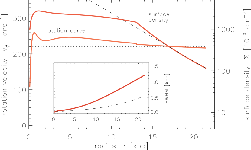
Figure 1: Midplane rotation curve (dotted line $=220\,\rm km\,s^{-1}$) and disc surface density. The inset shows the flaring scale-height of the HI gas disc. Dashed lines indicate observational approximations suggested by Kalberla & Dedes (2008).

We remark that the functional form of (6) is not differentiable at $R_{\rm br}$, which implies a slight jump in the azimuthal velocity, which we derive as

$$\bar{v}_{\phi}^{2}(R,z)=\left(\left.\frac{\partial\ln\bar{\varrho}}{\partial\ln R}\right|_{z=0}\!+q\,\right)\,c_{\rm s}^{2}+R\,\left.\frac{\partial\Phi}{\partial R}\right|_{z=0}+q\,\Phi_{z}(R,z)\,.$$ (9)

We note that, for $q\neq 0$, the last term will lead to a vertical variation of the rotation profile. Because the prescribed gravitational potential has been designed as a fit to the Galactic rotation curve, it suffices to say that (9) reproduces the classical Brandt-type curve with a plateau at $\bar{v}_{\phi}\simeq 220\,\rm km\,s^{-1}$ as also shown in Fig. 1, where we plot the rotation curve in the disc midplane. This completes the description of our hydrodynamic disc model. We have checked that the inviscid model can be evolved stably for times exceeding the age of the universe. When including turbulent viscosity, the disc evolves viscously on a secular time scale.

2.2 Turbulent closure parameters

Utilising a mean-field approach, we aim to simulate the common evolution of the regular magnetic field and the large-scale flow of the Galactic gas disc. Conceptually, this implies that we solve the full MHD equations subject to turbulent transport coefficients, i.e., we prescribe a turbulent diffusivity in the induction equation along with an according turbulent viscosity in the momentum equation. These turbulent dissipation coefficients, as well as the prescribed $\alpha$ effect (see Sect. 2.2.2), are derived from a series of resolved direct numerical simulations (DNS). The basic setup, which assumes a local box geometry and uses realistic driving of interstellar turbulence via injection of localised supernova explosions, is described in detail in Gressel (2009). Scaling relations for mean-field effects have been derived from a set of models with box size $0.8\,\rm kpc\times 0.8\,\rm kpc\times\pm 2.1\,\rm kpc$, and more accurate vertical shapes have been obtained using a larger $1.6\,\rm kpc\times 1.6\,\rm kpc\times\pm 6.4\,\rm kpc$ domain (Gressel et al., 2011). The requirement to resolve individual explosions demands grid resolutions below $10\,\rm pc$, which is met in the box simulations but will remain unaffordable in global simulations for some time.

Since in the DNS we only measure $\eta_{\rm t}$, but not $\nu_{\rm t}$, we have to assume a turbulent magnetic Prandtl number, $\mathrm{Pm}_{\rm t}=\nu_{\rm t}/\eta_{\rm t}$ of unity. This assumption is backed by recent numerical investigations that found very little deviation from this value (Guan & Gammie, 2009; Fromang & Stone, 2009). Note that unlike for a classical “$\alpha$” viscosity, we prescribe $\nu_{\rm t}(R,z)$ directly as a function of space, i.e., independent of the gas pressure. This is because (for consistency with the mean induction equation) we assume the turbulent velocity field to be given a priori as a consequence of the underlying SNe distribution. To avoid restrictive time-step constraints arising from high values of the diffusion coefficients, we have implemented the super-time-stepping scheme, introduced by Alexiades, Amiez, & Gremaud (1996), for the viscous and diffusive updates.

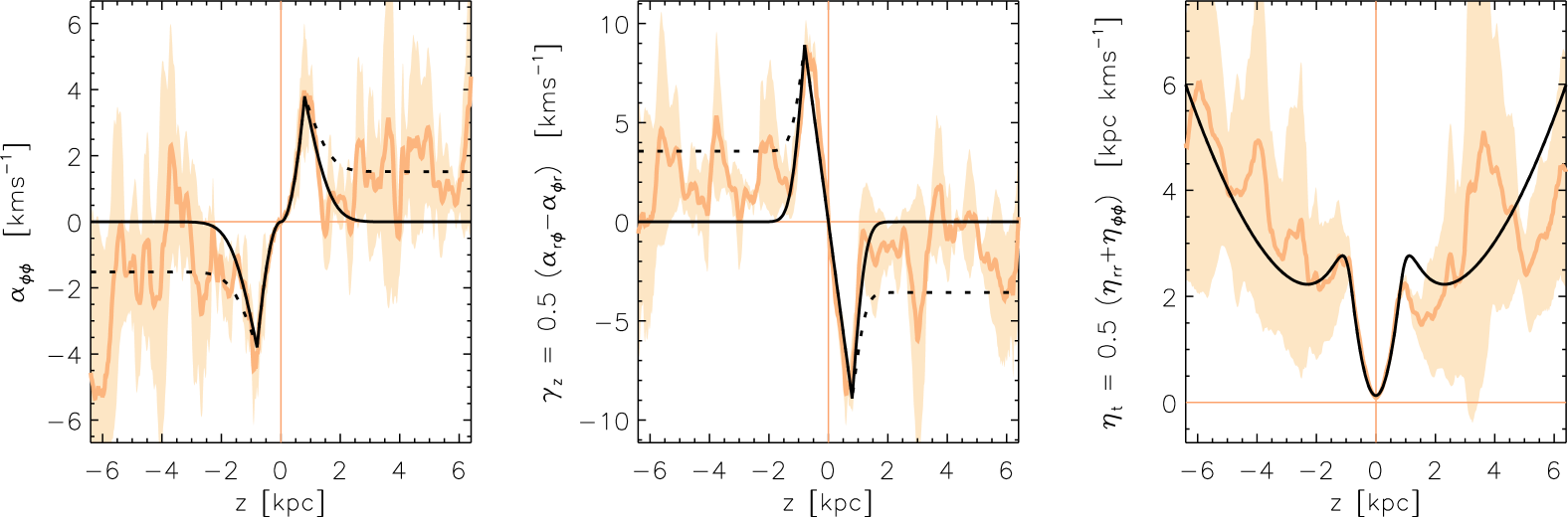
Figure 2: Vertical profiles of the TF coefficients $\alpha_{\phi\phi}$ (left), $\gamma_{z}$ (centre), and $\eta_{\rm t}$ (right panel) measured from DNS (light colours); shaded areas indicate $1\sigma$ fluctuations. Black curves show model profiles $\hat{\alpha}(\zeta)$, $\hat{\gamma}(\zeta)$, and $\hat{\eta}(\zeta)$ used for the simulation with (dashed line) and without (solid line) a halo dynamo.

2.2.1 Neglected effects

Turbulent viscosity is by no means the only mean-field effect in the momentum equation but, in fact, a crude oversimplification. For reasons of tractability, we however have to ignore more involved contributions like, e.g. the turbulent kinetic pressure or the turbulent contribution to the Lorentz force in our current considerations. A rudimentary attempt to allow the former effect to self-consistently launch a Galactic wind (driven by the gradient in the turbulence intensity) led to unacceptable mass-loss rates. This is because, in our mean-field model, the single-phase density field cannot properly capture the multi-phase nature of the ISM: Ultimately, what we described as a “wind” is really a “fountain flow”, i.e., tenuous gas being blown out of the Galaxy, while high-density clumps raining down compensate the overall mass balance. Ultimately, it will be of great interest to study related effects. We speculate that the suppression of the turbulent magnetic pressure by mean-fields (Kleeorin et al., 1989; Brandenburg et al., 2012a) may also be of importance in a Galactic context, potentially leading to an increased heterogeneity of the observed field (but also see Fletcher et al., 2009).

To be able to use periodic boundary conditions, an important simplification of our local box simulations was to ignore any large-scale radial structure in, e.g., the gas density or supernova rate. Even though we were able to vary quantities like the mid-plane density, rotation rate, or shearing rate for each of the individual runs (i.e. to adjust to the situation at different locations within the Galaxy), we could not obtain contributions in the dynamo tensor due to radial gradients.

2.2.2 The dynamo tensor

We here focus on a well-studied effect appearing in the mean induction equation, i.e., the turbulent electromotive force $\bar{\mbox{\boldmath{${\cal E}$}}}=\overline{\mathbf{v^{\prime}\!\times\!B^{\prime}}}$, where primes denote fluctuating quantities, and which we implemented by means of the classic tensor prescription

$$\bar{\mbox{\boldmath{${\cal E}$}}}_{i}=\alpha_{ij}\,\bar{B}_{j}\,\qquad i,j\,\in\left[r,\vartheta,\phi\right]$$ (10)

i.e., with an $\alpha$ tensor locally relating the mean EMF to the mean magnetic field. We argue that the good quantitative agreement between DNS and one-dimensional mean-field simulations (Gressel, 2009) warrants the neglect of non-local (Brandenburg et al., 2008) as well as non-instantaneous (Hubbard & Brandenburg, 2009) contributions to the closure. As laid out below, $\alpha_{ij}$ is parametrised according to coefficients measured within a comprehensive set of DNS of SN-driven ISM turbulence by means of the TF method (Schrinner et al., 2005, 2007).

Because of our flaring disc model, and for reasons of simplicity, we identify the $x$, $y$, and $z$ direction in these local Cartesian box simulations (Gressel et al., 2008a, 2009) with spherical polar coordinates $r$, $\phi$ (azimuth), and $\vartheta$ (co-latitude), respectively. To reflect the geometry of the disc, shape functions are defined with respect to a “flaring” coordinate $\zeta\equiv z/h(r)$, as to follow the local scale-height of the HI gas disc. At any spherical radius, $r$, the latitudinal variation is approximated by the profiles shown in Fig. 2. Note that (in accordance with our box model) the aspect ratio, $h(R)/R$, for the vertical profiles of the dynamo tensor is about a factor of two larger than the one for the HI disc shown in the inset of Fig. 2, resulting in a scale height of $\sim 1\,\rm kpc$ at $R\simeq 10\,\rm kpc$.

Table 1: Scaling exponents for the dynamo $\alpha$ tensor, the turbulent diffusivity and viscosity, and vertical fountain flow, $\overline{v}_{z}(\zeta)$. Amplitudes refer to shape functions $\hat{\alpha}(\zeta)$, $\hat{\gamma}(\zeta)$, and $\hat{\eta}(\zeta)$, which we matched to the TF profiles shown in Fig. 2 (also cf. Gressel, Elstner, & Rüdiger, 2011).

	amplitude    $\sigma/\sigma_{0}$			$\Omega/\Omega_{0}$	$\bar{\varrho}/\bar{\varrho}_{0}$
$\alpha_{\phi\phi}$	$2$	$\,\rm km\,s^{-1}$	0.4	0.5	-0.1
$\alpha_{\phi r}\,,-\alpha_{r\phi}$	$-12.5$	$\,\rm km\,s^{-1}$	0.45	-0.2	0.3
$\overline{v}_{z}$	8	$\,\rm km\,s^{-1}$	0.4	–	–
$\eta_{\rm t}\,,\nu_{\rm t}$	$2$	$\,\rm kpc\,\rm km\,s^{-1}$	0.4	0.25$\,{}^{a}$	0.4

^a) revised exponent from new analysis

The tensor components $\alpha_{rr}\simeq\alpha_{\phi\phi}\simeq 5\,\alpha_{\theta\theta}$, and $\alpha_{r\phi}\simeq-\alpha_{\phi r}$, which we directly measured in the DNS, are parametrised according to their inferred dependence on the supernova rate $\sigma/\sigma_{0}$, rotation rate $\Omega/\Omega_{0}$, and disc midplane density $\bar{\varrho}/\bar{\varrho}_{0}$. To further reduce the number of free parameters, we identify $\sigma/\sigma_{0}$ with the star formation rate, and link it to the local surface density by means of a Kennicutt-Schmidt law

$$\sigma/\sigma_{0}=(\bar{\varrho}/\bar{\varrho}_{0})^{1.4}$$ (11)

(Kennicutt, 1998). Scaling exponents are listed for reference in Table 1. Note that, for reasons of completeness, we include the radial and vertical diagonal elements of the tensor, even though we find these terms to be negligible compared to the $\alpha\Omega$ mechanism driven via $\alpha_{\phi\phi}$. Another important result from that paper was the existence of a vertical fountain flow, $\overline{v}_{z}$, which was discerned to balance the effect of the turbulent pumping. The vertical profile $\overline{v}_{z}(\zeta)$ which we adopt in our mean field prescription consists of two parts: a contribution linear in $\zeta$, and a characteristic modulation (cf. figure 2 in Gressel et al., 2009), which roughly coincides with $\alpha_{r\phi}(\zeta)$. It is important to note that the mean flow $\overline{v}_{z}$ – for reasons discussed in Sect. 2.2.1 – only contributes to the induction equation but is not included in the momentum equation.

2.2.3 Quenching functions

Avoiding a more complex description relating to the (approximate) conservation of magnetic helicity (see e.g. discussion in Moss & Sokoloff, 2011), we here resort to a simple algebraic expression for the $\alpha$ quenching as justified by our recent analysis (Gressel, Bendre, & Elstner, 2013). Unlike in many earlier studies, we explicitly include a quenching for the $\eta_{\rm t}$ (and $\nu_{\rm t}$) coefficient (also see Yousef et al., 2003). Adopting an isotropic quenching for the $\alpha$ tensor, we use

$$\alpha_{ij}(\bar{B})=\frac{\alpha_{ij}\,(\bar{B}\!=\!0)}{1+q_{\alpha}\,\beta^{2}}\,,\quad\nu_{\rm t}(\bar{B})=\eta_{\rm t}(\bar{B})=\frac{\eta_{\rm t}(\bar{B}\!=\!0)}{1+q_{\eta}\,\beta}$$ (12)

with $\beta\equiv|\bar{B}|/B_{\rm eq}$, and coefficients $q_{\alpha}=10$, and $q_{\eta}=5$ approximating the results from direct simulations (Gressel et al., 2013). Because of the close correspondence of $\alpha_{r\phi}$ and the characteristic modulation seen in the mean flow (cf. figure 3b in Gressel et al., 2013), we chose to apply quenching only to the modulation in $\bar{v}_{z}$, and leave the underlying linear profile unquenched.

For consistency, we moreover compute the equipartition field strength $B_{\rm eq}^{2}\equiv\mu_{0}\bar{\varrho}\,v_{\rm rms}^{2}$ from a turbulent velocity profile $v_{\rm rms}(\zeta)$ which has itself been derived from the (unquenched) $\eta_{\rm t}(\zeta)$ profile, assuming the classical relation $\eta_{\rm t}=\frac{1}{3}\tau_{\rm c}\,v_{\rm rms}^{2}$, and where we have used a constant $\tau_{\rm c}=3.5\,\rm Myr$ in consistence with DNS.

Note that it is essential that the $\alpha$ effect and the turbulent diffusion are quenched differently. This becomes obvious by evaluating $C_{\alpha}\equiv\alpha_{\phi\phi}h\eta_{\rm t}^{-1}$, and $C_{\Omega}=s\Omega h^{2}\eta_{\rm t}^{-1}$ (with $s\equiv{\rm d\,ln}\Omega/{\rm d\,ln}\,r$). Curiously, the resulting dynamo number $D\equiv C_{\alpha}C_{\Omega}$ is asymptotically independent of $|\overline{\mathbf{B}}|$. In practise, however, we have $q_{\alpha}>q_{\eta}$, which implies that $\alpha$ is quenched earlier. Estimating $\tan(p)\simeq(C_{\alpha}/C_{\Omega})^{1/2}\propto|\overline{\mathbf{B}}|^{-1}$, we see that a quenched $\alpha\Omega$ dynamo is dominated by differential rotation, leading to vanishing radial pitch angle. The loss of significant pitch angle in the saturated state can be circumvented if the dynamo is saturated at high $C_{\alpha}$ – e.g. via the vertical wind (see Elstner, Gressel, & Rüdiger, 2009).

3 Results

In the following, we will present results from a comprehensive suite of simulations. After we have attempted to eliminate as many as possible free parameters from our model, there remain only two major aspects that require testing: (i) the disc mass, i.e., the central input parameter governing the SF rate, and (ii) the initial topology of the magnetic field. Moreover, we aim to study non-axisymmetric modes, and whether the inclusion of the Navier-Stokes (NS) equation has an effect on the evolution of the Galaxy as a whole. In particular, we are interested in whether the MRI or convective instabilities can emerge on scales long enough not to be immediately affected by turbulent diffusion.

A compilation of the main results can be found in Table 2, where we also list the input parameters of our setup. Models labelled with ‘s’ are what we refer to as “static”, i.e. the density and velocity field are kept fixed during the evolution of the model. This is commonly assumed for the “kinematic” dynamo problem, albeit one of course includes a back-reaction of the field to obtain saturation of the dynamo. For some of the 3D models, we furthermore evolve the full MHD equations including the density and velocity field; these simulations are labelled ‘d’ for “dynamic”. For our fiducial axisymmetric (‘X’) model “X1s”, we vary the disc mass in steps of 0.5 times the fiducial mass of $1.14\times 10^{10}\,\rm M_{\odot}$ (see first four rows of Table 2). With models “X2s-halo” and “X3s-VF”, we study the influence of a halo dynamo and vertical-field seeding, respectively. The fiducial non-axisymmetric (‘N’) models “N1s” and “N1d” probe the effects of various seed-field geometries. With the exception of the two models “N2d-noD” (without any $\alpha$ effect, but including turbulent diffusion) and “N2d-MRI” (without any prescribed turbulence effects), all simulations include mean-field (MF) effects as described in Sect. 2.2 above. Generally, the MF dynamo remains dominant for these models, but subtle differences arise due to the long-term evolution of, e.g., the density distribution, which indirectly enters the MF prescription.

Table 2: Simulation parameters and results.

model

dim

MF

NS

halo

$M_{\rm gas}$

seed

parity

$p_{\rm in}$

$p_{\rm out}$

$\tau_{\rm e}$

$|\overline{\mathbf{B}}_{\rm sat}|$

comments

$\!\![10^{10}{\rm M_{\odot}}]\!\!$

$[\,\degr\,]$

$[\,\degr\,]$

$[{\rm Gyr}]$

$[\mu{\rm G}]$

X1s-0.5

2D

$\bullet$

$\circ$

$\circ$

0.57

WN

S0/A0

-11.6

-4.7

0.374

1.44

see Fig. 3

X1s

2D

$\bullet$

$\circ$

$\circ$

1.14

WN

S0a

-11.0

-4.6

0.503

3.75

see Figs. 4, 5

X1s-1.5

2D

$\bullet$

$\circ$

$\circ$

1.70

WN

S0a

-10.8

-4.6

0.547

6.34

X1s-2.0

2D

$\bullet$

$\circ$

$\circ$

2.27

WN

S0

-10.7

-4.3

0.593

9.07

X2s-halo

2D

$\bullet$

$\circ$

$\bullet$

1.14

WN

S0a

-11.7

-4.8

0.358

4.05

X3s-VF

2D

$\bullet$

$\circ$

$\circ$

1.14

VF

A0$\rightarrow$S0

-11.0

-4.5

0.539

3.75

N1s/d-HF $\ \ \left<\frac{}{}\right.$

3D

$\bullet$

$\circ$

$\circ$

1.14

HF

S0

-11.0

-3.2

–

3.75

3D

$\bullet$

$\bullet$

$\circ$

1.14

S0

- 9.9

-2.6

–

2.52

N1s/d-VF $\ \ \left<\frac{}{}\right.$

3D

$\bullet$

$\circ$

$\circ$

1.14

VF, $\bar{B}_{\phi}$

S0

-11.0

-6.1

0.409

3.75

3D

$\bullet$

$\bullet$

$\circ$

1.14

S0

- 9.9

-2.7

0.407

2.65

see Fig. 12

N2d-noD

3D

$\circ$b

$\bullet$

$\circ$

1.14

HF+VF

A0

-1.7

-1.6

–

0.82c

see Fig. 7

N2d-MRI

3D

$\circ$

$\bullet$

$\circ$

1.14

HF+VF

A0

-0.4

-0.5

–

4.25

see Fig. 7

N3d-VF

3D

$\bullet$

$\bullet$

$\circ$

1.14

VF

S0/A0

-10.2

-3.4

–

3.46

see Figs. 7, 9, 10

^a sub-dominant A0 outside $R\simeq 10\,\rm kpc$, $\quad{}^{b}$ includes $\eta_{\rm t}$, and $\nu_{\rm t}$, $\quad{}^{c}$ obtained outside $R\simeq 15\,\rm kpc$.
All 2D runs are axisymmetric; mean-field (MF) effects include the ones described in Sect. 2.2; runs including ’NS’ evolve the Navier-Stokes equation. The ‘halo’ dynamo is shown as a dashed line in Fig. 2. The column labelled $M_{\rm gas}$ gives the normalisation for the disc mass. For seed fields we use white noise (WN) with $0.15\,\rm nG$ rms amplitude, net-vertical field (VF) of $0.1\,\rm nG$, or net-horizontal field (HF) of $0.01\,\mu\rm G$. Pitch angles are given for the inner disc (i.e., where the magnetic field strength peaks) and for the outer disc (average for $R>10\,\rm kpc$) separately. Growth rates are for the magnetic field $|\overline{\mathbf{B}}|$, during an interval for which exponential growth can be identified.

To be as unrestrictive as possible on the emerging dynamo mode, we generally apply a white-noise (WN) initial field, resulting in approximately equal amounts of energy in all permissive modes. Moreover, for the 2D models, we alternatively apply a net-vertical field (VF), which might be hypothesised as a plausible seed topology. Finally, in the 3D case, it furthermore becomes possible to test a configuration with initially horizontal field (HF); even though this topology is generally found to be impractical due to the winding-up effect of the differential rotation (Moss & Sokoloff, 2012).

3.1 Vertical parity and growth rates

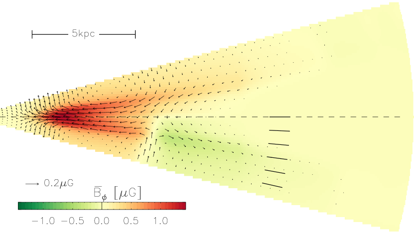
Figure 3: Saturated regular magnetic field for model X1s-0.5; colour-coded toroidal field, $\bar{B_{\phi}}$, overlaid vectors show the poloidal field. Short line segments indicate the latitudinal positions of slices in Fig. 5, below.

In agreement with many previous studies (see e.g. Beck et al., 1996), we find the axisymmetric (i.e., $m=0$, hence “0”) mode with symmetric vertical parity (“S”) as the fastest growing dynamo mode (see column 8 in Table 2). Notably, in the low-density part of the disc (beyond $R\simeq 10\,\rm kpc$), a weak anti-symmetric (“A”) mode emerges. This is illustrated in Fig. 3, which shows the saturated magnetic field for model X1s-0.5 (with lower disc mass), where the A0 mode is seen most pronounced. Possible reasons for this may be a combination of pumping and wind, as well as the disk flaring. In most models, the A0 contribution remains sub-dominant, but appears during a transitional phase in the case of a vertical-field initial condition (e.g. model X3s-VF). Note that the mixed S0+A0 leads to a radially confined, strong vertical field on only one side of the Galactic disc. This is consistent with radio observations of extragalactic Faraday rotation at high Galactic latitude by Mao et al. (2010), who find a vertical field consistent with $(0.00\pm 0.02)\,\mu\rm G$ towards the north, and $(0.31\pm 0.03)\,\mu\rm G$ towards the south Galactic pole, respectively.

Exponential growth times of the mean-field dynamo are presented in column 11 of Table 2. Generally, we find $\tau_{\rm e}$ on the order of half a ${\rm Gyr}$, which is sufficient to explain the present-day field strength of the Galaxy based on reasonable assumptions on the initial seed field. Neronov & Vovk (2010) estimated from Fermi observations a lower bound of of $3\times 10^{-16}\,{\rm G}$ for the intergalactic field on ${\rm Mpc}$ scales. A possible explanation of the generation process was recently given by Schlickeiser (2012). The formation of the protogalaxy leads to a further amplification up to $3\times 10^{-12}\,{\rm G}$ (Lesch & Chiba, 1995), so roughly after $7\,\rm Gyr$ the dynamo has equipartition field strength of several microgauss. Prior to the epoch of star formation, the MRI may grow unhindered by turbulence from SNe and hence serve as a seed-field mechanism as suggested by Kitchatinov & Rüdiger (2004).

For the fiducial model X1s, we find a trend to faster growth for lighter disc models. This is presumably due to the reduced turbulent diffusivity at lower SF activity. For lighter disc models we also expect the wind to dominate over the vertical pumping, resulting in weaker saturated fields and larger magnetic pitch angles. The fastest growth of $\tau_{\rm e}=0.358\,\rm Gyr$ is found in model X2s-halo, including a non-zero $\alpha$ effect at high Galactic latitude (cf. dashed line in Fig. 2). Compared to the standard model X1s, which is seeded from white noise, model X3s-VF with a vertical-field initial condition shows a slightly slower growth rate of $\tau_{\rm e}=0.539$, which can be identified with the A0 eigenmode. Faster growth can be obtained if one starts with the S0 mode directly – cf. model N1s-VF, where a combined vertical and azimuthal field is applied.

3.2 Radial structure

The amount of quantitative information that can be confidently extracted from radio observations of the Milky Way or nearby galaxies is rather limited. In particular, reliable positional information is restricted to considering the radial variation of azimuthally and vertically averaged quantities. In the interest of direct quantitative comparison with observations, we here want to discuss the magnetic field strength and its inclination with respect to the toroidal direction.

3.2.1 The magnetic pitch angle

One major observable derived from radio polarisation maps is the radial pitch angle, $p\equiv\tan^{-1}(\bar{B}_{R}/\bar{B}_{\phi})$ of the mean magnetic field. Because values of $|p|\,\hbox{\lower 1.50696pt\hbox{$\sim$}\hbox to0.0pt{\hss\raise 1.50696pt\hbox{$>$}}}\,10\degr$ are hard to explain in the presence of differential rotation alone, large pitch angles are generally interpreted as the hallmark of an $\alpha$ effect dynamo. Our models generally show moderately large pitch angles close to $-10\degr$ (see column 9 of Table 2) in the inner region of the Galactic disc, i.e. where the magnetic energy is highest. The models N1d-HF/VF, including evolution of the disc, show somewhat reduced pitch angles. This may be related to the long-term viscous evolution of the radial gas density profile, which reduces the SF rate entering our dynamo prescription, and hence the strength of the MF dynamo near the Galactic centre. It is interesting to note that we do not see a significant change of pitch angle during the simulation – implying a saturation at high $C_{\alpha}$, likely due to the action of the vertical fountain flow (cf. Elstner et al., 2009).

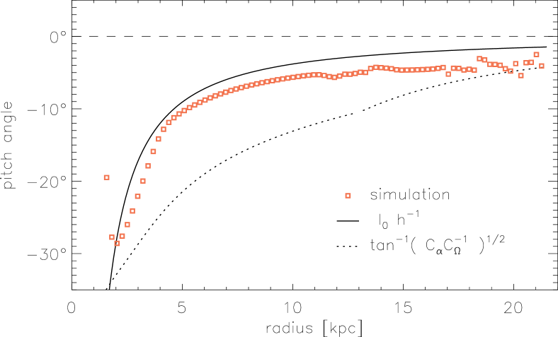
Figure 4: Radial pitch angle $p\equiv\tan^{-1}(\bar{B}_{R}/\bar{B}_{\phi})$ for model X1s at the end of the simulation. The observed radial trend is well approximated by the crude estimate $p\simeq l_{0}\,h^{-1}$ (Fletcher, 2010), with $l_{0}=120\,\rm pc$.

Fletcher (2010) points out the systematic variation of the magnetic pitch angle with radius, which he ascribes to the flaring of the disc. Similarly, Rae & Brown (2010) have observed a vanishingly small pitch angle for the outer Galaxy. In Figure 4, we plot the radial profile of the pitch angle (in the disc midplane) for the fiducial model X1s. The large angles of the order of $-30\degr$ in the inner part should be ignored since the mean field is significant below the equipartition value there (cf. Fig. 5 below), which should make them very hard to detect in polarised synchrotron emission. Consistent with observations (see e.g. fig. 4 in Fletcher, 2010), the pitch angle in our simulations decreases roughly like $R^{-1}$. Crudely estimating $p\simeq l_{0}\,h^{-1}$, with a correlation length, $l_{0}$, of the turbulence, this behaviour can conveniently be explained by the flaring of the gas disc (cf. Fig 1). The good match is somewhat deceiving as the supposedly more accurate estimate

$$p\simeq\tan^{-1}\sqrt{C_{\alpha}\,C_{\Omega}^{-1}}$$ (13)

in fact provides a much poorer description of the actual result. Whereas Fig. 4 shows the pitch angle in the Galactic midplane, the peculiar shape of the dynamo A0 mode in the outer Galaxy (seen in Fig. 3 above) suggests to look at latitudinal slices away from the midplane – and, in fact, the pitch angle of the A0 mode follows Eqn. (13) more closely. Concluding this section, we want to point out that the two models N2d-noD and N2d-MRI without prescribed dynamo action produce vanishingly small pitch angles. This is likely because the initial magnetic field is rather small and accordingly the unstable modes lie close to the diffusive border of the unstable region. In this case, the unstable mode is characterised by a dominant toroidal field (Kitchatinov & Rüdiger, 2004). The pitch angle is however larger for model N3d-VF with the stronger initial field of $0.1\,\mu\rm G$.

3.2.2 The saturated field strength

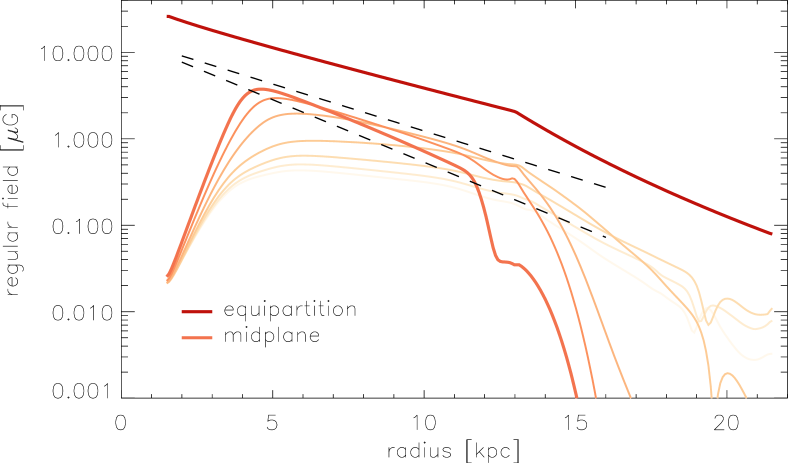
Figure 5: Saturated regular magnetic field for model X1s for various cuts of constant co-latitude. The midplane field peaks at about $4\,\mu\rm G$. Dashed lines show exponentials with scale lengths of 3 and $4\,\rm kpc$, respectively.

Most of the nearby spiral galaxies are believed to be observed in the saturated state of the dynamo (Beck et al., 1996). With increasingly detailed observations, it becomes possible to determine the radial profile of the field strength (see e.g. Beck, 2007). Based on this, one can then estimate the relative importance of magnetic forces on the overall rotational balance within the Galactic disc (see Sánchez-Salcedo & Santillán, 2013). Because we have started from a quantitative disc model, we can hope to make meaningful predictions about the radial distribution of magnetic field. Accordingly, in Fig. 5 we present radial profiles of the fiducial model X1s in the saturated state. As one can see in Fig. 3 above, the dominant dynamo mode has a characteristic V-shape, which makes it instructive to plot radial cuts at various angles $\theta$ away from the midplane. The different curves are within $0-15\degr$ below the midplane (in steps of $\delta_{\theta}=2.5\degr$) and cuts further away from the midplane are shown in increasingly lighter colour. The positions of the cuts are also indicated in Fig. 3 by short line segments. The profiles are steepest near the midplane, and roughly follow exponential curves with scale lengths between $3-4\,\rm kpc$ as indicated by dashed lines in Fig. 5. This scale appears to be partly inherited from the equipartition profile, which is itself a consequence of the disc model and the scaling relations entering via $\eta_{\rm t}(r,\theta)$. Owing to the rather restrictive quenching factor of $q_{\alpha}=10$, our dynamo solutions remain well below equipartition strength (dark line), but peak values of a few microgauss are nevertheless obtained (see column 12 in Table 2). The final field strength shows substantial variation, illustrating the dependence on the disc model. The highest absolute value (i.e., $9\,\mu\rm G$) of the mean field is found in the high disc mass case – with a trend to weaker fields for less massive gas discs. This trend also explains the lower saturated field strength of $\simeq 2.5\,\mu\rm G$ in model N1d-HF (and similarly N1d-VF) compared to $\simeq 3.8\,\mu\rm G$ in N1s-HF (and N1s-VF), which does not include the evolution of the disc’s surface density.

3.3 The role of dynamical instabilities

One key aspect of the simulations presented in this paper is the inclusion of the Navier-Stokes equations in the modelling, enabling us to capture dynamical instabilities occurring on large length scales. It has been suggested by Sellwood & Balbus (1999) that turbulence created via MRI may play a role in the outer Galactic disc, i.e., in the absence of significant star-formation activity and the associated enhanced diffusion. In view of this, it is interesting to study the hypothetical case of a Galactic disc without any star-formation activity, for which one can perform simple MHD simulations without any prescribed mean-field effects from unresolved scales (see e.g. Dziourkevitch et al., 2004; Machida et al., 2013). Such simulations should however be interpreted with care since they neglect the dominant source of energy input to the system, namely that from SNe.

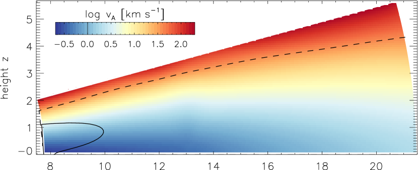
Figure 6: Vertical-field Alfvén speed for the initial configuration of model N3d-VF (with $B_{z}=0.1\,\mu\rm G$), along with marginal stability lines according to the diffusive limit (solid) and strong-field limit (dashed line), represented by the left- and right-hand side of (14), respectively.

The occurrence of MRI – subject to pre-existing turbulence from SNe – can easily be gauged from linear theory. According to the local criterion derived in Appendix A of Kitchatinov & Rüdiger (2004), who study the linear stability of MRI in a global cylindrical disc of semi-thickness $H$, instability is obtained within a range

$$\sqrt{\frac{2-s}{s}}\ \frac{\eta_{\rm t}}{H}\ \,\hbox{\lower 1.50696pt\hbox{$\sim$}\hbox to0.0pt{\hss\raise 1.50696pt\hbox{$<$}}}\,\ v_{\rm A}\ \,\hbox{\lower 1.50696pt\hbox{$\sim$}\hbox to0.0pt{\hss\raise 1.50696pt\hbox{$<$}}}\,\ \sqrt{2s}\ H\Omega\,,$$ (14)

where $v_{\rm A}\equiv|B_{z}|\,\rho^{-1/2}$ is with respect to the vertical field. For a flat rotation curve with $s=1$, this yields $\eta_{\rm t}\,H^{-1}<v_{\rm A}<1.4H\Omega$, implying that already for $C_{\Omega}>1$, there exists a magnetic field unstable to MRI. This is illustrated in Fig. 6, where we show the marginal stability lines for our model N3d-VF with a moderately strong initial field of $0.1\,\mu\rm G$. For $R\,\hbox{\lower 1.50696pt\hbox{$\sim$}\hbox to0.0pt{\hss\raise 1.50696pt\hbox{$<$}}}\,8\,\rm kpc$, the region of possible MRI activity is significantly restricted, whereas the outer disc clearly shows the potential to develop the instability.

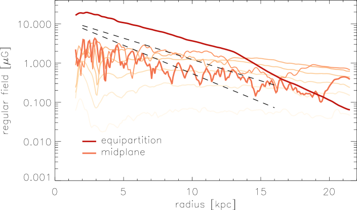
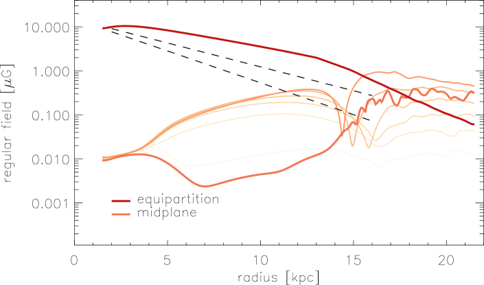
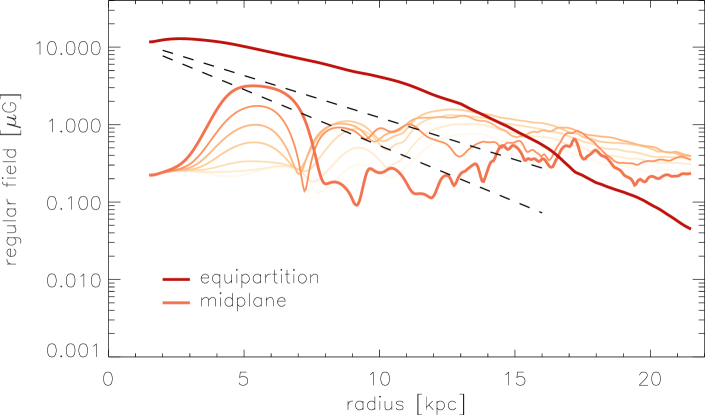
Figure 7: Same as Fig. 5 but for different dynamical models. Top panel: Model N2d-MRI without prescribed MF effects; the radial scale length of the magnetic field is $\simeq 10\,\rm kpc$. Middle panel: Model N2d-noD without $\alpha$ effect but including turbulent diffusion (which suppresses the MRI for $R\,\hbox{\lower 1.50696pt\hbox{$\sim$}\hbox to0.0pt{\hss\raise 1.50696pt\hbox{$<$}}}\,15\,\rm kpc$). Bottom panel: Model N3d with combined $\alpha$ effect and MRI, at $t=3.9\,\rm Gyr$, i.e., when the S0 mode dominates (cf. Fig. 9b).

In the three panels of Fig. 7, we try to illustrate the interplay of prescribed small-scale effects with dynamical instabilities. In the upper panel of that figure, we present model N2d-MRI, where no dynamo-effects or turbulent diffusivity have been prescribed, and where dynamo activity is due to magnetic instabilities such as the MRI and convection. This case corresponds to the MHD simulations of Machida et al. (2013). In contrast to the static dynamo simulation discussed earlier (see Fig. 5), it is worth mentioning that in this case one obtains a much flatter radial dependence of the mean magnetic field strength which is in better agreement with observations (see e.g. Beck, 2007, which is however for the external galaxy NGC 6946).

Because isolated MRI is a highly idealised scenario, we now turn to the more realistic case where the MRI is affected by turbulence resulting from SNe. In a general context, the effect of Ohmic diffusion on growing MRI modes has been studied in the framework of linear perturbation (Jin, 1996), and based on this, Gressel et al. (2008b) have argued that the turbulent diffusion from SNe should be sufficient to damp the MRI at the solar radius (also cf. Fig. 6 above). Whether simple picture of “enhanced” diffusion is viable needs to be scrutinised. Simulations combining hydrodynamic forcing with the non-linear evolution of the MRI (Workman & Armitage, 2008), produce a rather varied picture. However, for moderately strong small-scale forcing, the authors indeed conclude that MRI may be suppressed by preexisting turbulence. A similar conclusion is reached by Korpi et al. (2010), who run shearing-box simulations with finite Ohmic resistivity and, alternatively, with small-scale forcing. The authors demonstrate that, assuming a typical $\eta_{\rm t}(R)$, MRI turbulence can be sustained inside the Galactic disc outside $R\simeq 14\,\rm kpc$. This finding turns out to be in excellent agreement with our model N2d-noD, where we apply turbulent diffusion (and viscosity), but disable the mean-field dynamo. The resulting radial field profiles are plotted in the middle panel of Fig. 7.

As an aside, we note that, in MRI turbulence, the velocity dispersion is typically found to be linked to the Alfvén speed (Dziourkevitch et al., 2004). As can be seen in Fig. 7, outside $\simeq 15\,\rm kpc$ the MRI indeed leads to super-equipartition field strengths with respect to the turbulent kinetic energy input from SNe. Furthermore, in agreement with the profiles obtained for NGC 6946 (Beck, 2007), the radial scale length of the regular field exceeds the scale length of the turbulence – this is unlikely for the dynamo-only case (cf. Fig. 5).

Regarding the general field morphology (also see Sect. 3.4 below), we find that anti-symmetric parity of the emerging mean field prevails. This is despite linear theory predicts quadrupolar-like, i.e. S0, parity (Kitchatinov & Rüdiger, 2004) for MRI (albeit for a non-flaring disc of constant thickness). Because of the dominance of the A0 mode, the peak value of approximately $1\,\mu\rm G$ is reached away from the disc midplane. Returning to the importance of pre-existing turbulence, we want to emphasise that for model N2d-noD, turbulent diffusion dominates in the inner disc (i.e., for $R\,\hbox{\lower 1.50696pt\hbox{$\sim$}\hbox to0.0pt{\hss\raise 1.50696pt\hbox{$<$}}}\,15\,\rm kpc$); there the mean magnetic field remains at the initial seed-field level. Away from the disc midplane, where the prescribed turbulent diffusion is stronger, field is diffused-in from the MRI-active outer region.

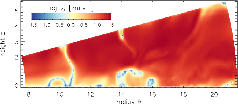
Figure 8: Alfvén velocity based on the azimuthal field, $\bar{B_{\phi}}$, for model N3d-VF at time $t=3.9\,\rm Gyr$. Velocities are surprisingly uniform reaching moderate values of several tens of $\rm km\,s^{-1}$.

Both of the two previously described scenarios only tell part of the story. The models without any explicit mean-field effects (upper panel of Fig. 7), and without $\alpha$ effect (middle panel), instead should be contrasted with the case of a combined evolution of mean-field effects and dynamical instabilities on large scales – this is shown in the lower panel of the same figure. In the inner disc ($R\,\hbox{\lower 1.50696pt\hbox{$\sim$}\hbox to0.0pt{\hss\raise 1.50696pt\hbox{$<$}}}\,8\,\rm kpc$), the S0 dynamo mode prevails, with strong fields near the midplane. In the range $8\,\rm kpc\,\hbox{\lower 1.50696pt\hbox{$\sim$}\hbox to0.0pt{\hss\raise 1.50696pt\hbox{$<$}}}\,R\,\hbox{\lower 1.50696pt\hbox{$\sim$}\hbox to0.0pt{\hss\raise 1.50696pt\hbox{$<$}}}\,10\,\rm kpc$, the A0 dynamo mode results in weak fields near $z=0$, whereas for $R\,\hbox{\lower 1.50696pt\hbox{$\sim$}\hbox to0.0pt{\hss\raise 1.50696pt\hbox{$>$}}}\,14\,\rm kpc$ the magnetic field is mostly due to MRI activity. Unlike in the case without prescribed dynamo effects, at late times, i.e., after $t=3.9\,\rm Gyr$, the MRI now reaches in to about $R\,\hbox{\lower 1.50696pt\hbox{$\sim$}\hbox to0.0pt{\hss\raise 1.50696pt\hbox{$>$}}}\,9\,\rm kpc$ – probably assisted by field-amplification via the $\alpha$ effect dynamo. Observationally, the resulting radial scale length would likely appear considerably larger than for a pure dynamo field (cf. Fig. 5 above).

Returning to the question concerning effects of the regular magnetic field on the Galactic rotation curve (see Sánchez-Salcedo & Santillán, 2013), we point out that the relative importance of magnetic fields in the overall force balance can be roughly estimated by considering the strength of the field with respect to the gas density. Accordingly, in Fig. 8, we plot the azimuthal-field Alfvén velocity for the third case discussed above. Most notably, $v_{\rm A}$ is very uniform throughout the outer Galactic disc. With values of several tens of $\rm km\,s^{-1}$, the effect of the Lorentz force on the rotation curve is likely to remain low and within current observational uncertainties. Near the magnetic reversal at $R\simeq 10\,\rm kpc$, a minor deviation of $\simeq+10\,\rm km\,s^{-1}$ is seen in the rotational velocity at intermediate Galactic latitude. Such a potential correlation between a field reversal and a peak in the rotation curve may be a promising future target for combined optical and radio-polarimetric observations.

3.4 Morphology of fully dynamical discs

(a)

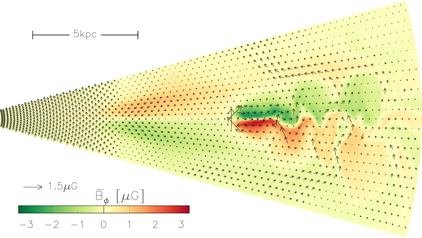
(b)

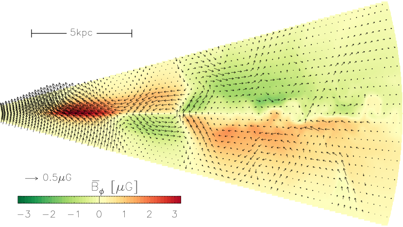
Figure 9: Poloidal cuts through model N3d-VF, with colour-coded $\bar{B}_{\phi}$ and vectors indicating the in-plane field. Panel (a), at $t=2.7\,\rm Gyr$, shows the initial A0 mode and strong fields created by the combined action of MRI and convection outside $R\simeq 10\,\rm kpc$. In panel (b), at $t=3.9\,\rm Gyr$, the S0 appears, and MRI is now somewhat weaker.

The emergence of the MRI in our simulations is limited by various factors. Weak seed fields, for example, imply that the plasma parameter $\beta_{\rm P}\equiv 2\bar{p}/\bar{B}^{2}$ falls into a range where MRI only appears at high wavenumbers and only far up in the disc where the gas pressure is low. To circumvent limitations due to insufficient numerical resolution, we ran an additional scenario “N3d-VF”, which is identical to N1d-VF, but has a higher initial net-vertical magnetic field of $B_{z}=0.1\,\mu\rm G$, and adopts a higher resolution of $384\times 72\times 96$ grid cells. With this model, we aim to study the combined effects of the mean-field dynamo and secondary instabilities, as already illustrated in the previous section.

A more detailed evolution of this model is presented in Fig. 9, where we show vertical cuts through the domain. Note that the $\bar{B}_{\phi}$ field created by the MRI (visible in the outer disc) has the opposite polarity than the A0 dynamo mode (seen between $5\,\rm kpc\,\hbox{\lower 1.50696pt\hbox{$\sim$}\hbox to0.0pt{\hss\raise 1.50696pt\hbox{$<$}}}\,R\,\hbox{\lower 1.50696pt\hbox{$\sim$}\hbox to0.0pt{\hss\raise 1.50696pt\hbox{$<$}}}\,10\,\rm kpc$). This leads to a distinct radius where the field is zero (which is also clearly visible in the derived polarisation map – see Fig. 12 below). While this would provide a natural explanation for the observed field reversal in our own Galaxy, it is currently not clear whether the antagonism between the MRI mode and the dynamo mode is random or systematic in our model. A careful study of what determines the prevalent mode structure in the presence of combined MRI and mean-field effects is certainly called for.

Owing to the lower $\beta_{\rm P}$, the MRI develops closer to the disc midplane. There the density is strongly stratified, which in turn seems to lead to a Parker-type convective instability (Newcomb, 1961; Foglizzo & Tagger, 1994, 1995) visible in the form of field arcs. Note that the vertical undulation of the antisymmetric $\bar{B}_{\phi}$ creates apparent radial reversals of the field direction in the disc midplane. It would be interesting to check whether such a field distribution is consistent with all-sky data of Faraday rotation and polarised emission (see e.g. Jaffe et al., 2010). Clearly, this type of reversal would be very difficult to observe in external galaxies – which may conveniently explain why the Milky Way appears unusual in this regard.

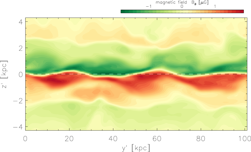
Figure 10: Projected $\theta$-$\phi$-slice of the azimuthal magnetic field at $r=16\,\rm kpc$. The dominant wavelength along the field lines is on the order of $30\,\rm kpc$.

Our claim that a Parker-like buoyant instability is operating in the regions of strong field creation has so far largely been guided by visual appearance. In the following we hence try to assess, in a semi-quantitative manner, the requirements for buoyancy instabilities to occur. It is well established that the convective instability (Newcomb, 1961) works to interchange neighbouring segments of field lines. Because magnetic tension forces oppose line bending, the interchange will preferably occur on long segments. With dominant $\bar{B}_{\phi}$ fields, one would thus expect perturbations that have higher wave numbers in the radial direction compared to the azimuthal direction. This is illustrated for model N3d-VF in Fig. 10, where we show a $\theta$-$\phi$ slice of the $\bar{B}_{\phi}$ field component (for the same point in time as for panel (a) in Fig. 9). Note that Fig. 10 does not preserve aspect ratio and the azimuthal coordinate $y^{\prime}$ is strongly compressed compared to the poloidal slice in the previous figure. The dominant azimuthal mode appears to be $m=3$, which corresponds to a wavelength of $\lambda_{y}\simeq 30\,\rm kpc$. In agreement with local simulations by Johansen & Levin (2008), this is about a factor of 10–20 larger than the radial wavelength $\lambda_{x}\simeq 2\,\rm kpc$. By order of magnitude (Newcomb, 1961), one would expect $2\pi L/\lambda_{y}\sim 1$, where $L$ is the scale height of the total pressure $\bar{p}^{\star}\equiv\bar{p}+\bar{B}^{2}/2$. In agreement with this estimate, we infer a value of $L\simeq 5\,\rm kpc$. Based on our simulation data, we moreover evaluate the basic stability criterion for convective stability (assuming $\gamma=1$), the fastest growing wave number ($\lambda_{y}\sim 10\,\rm kpc$), and growth rates ($\tau_{\rm e}\sim 100\,\rm Myr$). While a quantitative comparison is hampered by the fact that we cannot isolate the unperturbed background state, the overall numbers support the notion that convective perturbations in the disc are indeed created by magnetic buoyancy. We point out that the inclusion of a non-isothermal equation of state may have a stabilising effect on the system, which means that our current models may overestimate related effects. On the other hand, this type of instability has been argued to be enhanced by the presence of a cosmic-ray component (Parker, 1992; Hanasz et al., 2004). As a concluding remark, we note that observational support for such buoyant arcs remains largely unavailable – although claims have been made for magnetic loops in the inner Galactic disc (Fukui et al., 2006).

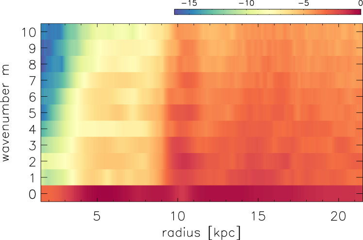
Figure 11: Logarithmic power spectrum of $\bar{B}_{\phi}$ as function of radius for model N3d-VF at time $t=3.9\,\rm Gyr$. The dynamo field is purely axisymmetric, whereas outside $R\simeq 9\,\rm kpc$ MRI turbulence is able to produce significant non-axisymmetric features.

To illustrate the very distinctive character of the dynamo-generated field on one hand, and the field resulting from dynamical magnetic instabilities on the other hand, in Fig. 11, we show the vertically-averaged azimuthal power spectrum of the magnetic field. The spectrum is taken from model N3d-VF at time $t=3.9\,\rm Gyr$, and has been normalised to a maximum of one. The logarithmic colour coding spans the available dynamic range of the double-precision floating point numbers used in the simulation, ranging from essentially zero (blue) to the maximum (dark red). The dynamo field is characterised by a perfectly axisymmetric $m=0$ mode. Outside $R\simeq 9\,\rm kpc$, we find significant non-axisymmetric modes, but without any particular mode number dominating. In the transition region between the $\alpha\Omega$ dynamo and the MRI-dominated region, we see power at odd overtones as well as a peak at $m=2$.

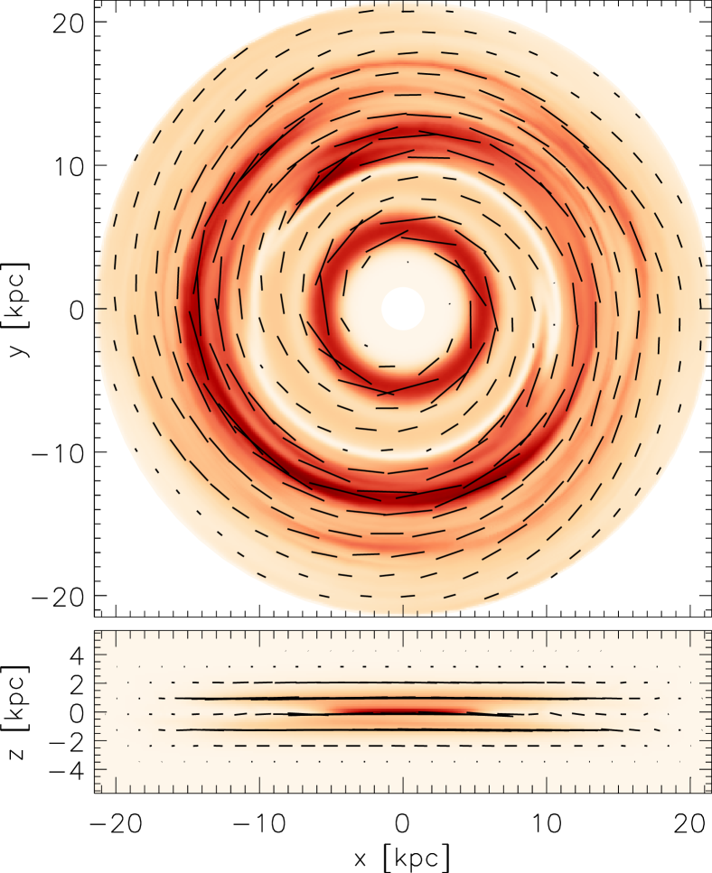
Figure 12: Synthetic polarisation maps for model N3d-VF at $t=3.9\,\rm Gyr$, i.e., corresponding to the lower panel in Fig. 9. Colour coding shows the Stokes-I parameter, and compass needles indicate the direction of polarisation (rotated by $90\degr$).

This feature is also seen in Fig. 12, where we show a very basic polarisation map created from the saturated state of model N3d-VF. This synthetic radio map integrates polarised synchrotron emission along the line of sight, ignoring effects of Faraday-rotation and -depolarisation, and assuming a flaring disc (of scale height $h_{\rm rel}=1.5\,\rm kpc$ at $R=10\,\rm kpc$) for the density $n_{\rm rel}$ of relativistic electrons. In the edge-on projection, we infer a radial scale length of the total intensity of about $5\,\rm kpc$ if we assume a radially constant $n_{\rm rel}$. If we assume a correlation $n_{\rm rel}\propto\bar{B}^{2}$, this is naturally reduced to $2.5\,\rm kpc$. Needless to say that both results are consistent with the radial scale length of $10\,\rm kpc$ seen for the magnetic field in Fig. 7. We remark that these estimates refer to the strong fields created in the outer disc by the MRI in combination with buoyancy and the mean-field dynamo. We conclude that a potential field reversal at a mode interface will make it difficult to infer a meaningful global scale length from observations. This is in any case difficult for the Milky Way itself, but slightly larger values have, e.g., been obtained for NGC 6946 (Beck, 2007), where a scale length of $14\,\rm kpc$ has been found for the total magnetic field.

Ultimately, we aim to compare polarisation maps such as in Fig. 12 to observation-based models for the Galactic magnetic field, e.g., the face-on view (top panel) of the heuristic model derived by Jansson & Farrar (2012a); their figure 9. We see that our dynamo field is less centrally-confined than the best-fit to the all-sky polarisation maps, and obviously lacks the precise spiral features. More significantly, in the edge-on view (see lower panel of Fig. 12), we do not see any X-shaped field topology. Even though our dynamo models do produce significant vertical field, these are always dominated by stronger radial and azimuthal fields. In the edge-on projection, the polarisation vectors are accordingly aligned with the horizontal direction.

4 Summary of results

With mean-field coefficients calibrated from direct SN simulations (see Table 1), and with quenching functions determined quantitatively (Gressel et al., 2013), we are left with essentially no free input parameters other than the initial geometry of the magnetic seed field. This of course precludes the possibility to derive a bifurcation diagram for dynamo modes or critical dynamo numbers (Brandenburg et al., 1992). On the other hand, it is satisfying that, without tuning of any parameters, the outcome of our simulations is indeed in decent agreement with observational constraints.

• In all our models, we find a dominant S0 mode for the dynamo, but with a sub-dominant A0 mode situated in the outer disc. In the case of a low disc mass, the A0 mode is most pronounced. We moreover find anti-symmetric parity (notably of the opposite sign) for the dominant MRI mode.

• The mixed S0+A0 dynamo mode leads to a localised region of strong vertical field, which is enforced by the requirement of a zero divergence. Because of the mixed parity, the vertical field only appears on one side of the disc, as is consistent with recent observations by Mao et al. (2010).

• Consistent with a topical compilation of observations by Fletcher (2010), the radial profile of the magnetic pitch angle emerging from our model decreases with inverse radius. This is very well approximated by $p\simeq l_{0}h^{-1}$, with $h$ the local scale-height of the flaring disc.

• Vertical undulations caused by magnetic instabilities, in connection with an anti-symmetric vertical parity, can create apparent radial reversals near the disc midplane. The resulting field topology should be tested against available data of rotation measures in the Galactic plane. A reversal is also seen at the interface between the dynamo and MRI modes.

• The most pronounced effect of allowing magnetic instabilities is to significantly enhance the radial scale length of the magnetic energy in the outer disc. Such shallow profiles, where the scale length of the field exceeds the one of the turbulence, have been observed in NGC 6946 (Beck, 2007).

• There has been renewed interest in the radial dependence of the magnetic field strength and its influence on the rotation curve (Sánchez-Salcedo & Santillán, 2013). In our dynamo models, we find exponential scale lengths of $\sim 3-4\,\rm kpc$, which is somewhat shorter than expected. A shallower radial profile is seen in the disc halo, as well as in cases where the MRI leads to strong fields in the outer disc. Even there, deviations from the initial rotation curve stay well below current observational uncertainties.

5 Conclusions

We have described a new, comprehensive modelling approach for global mean-field simulations of the Galactic dynamo. To be able to make quantitative predictions, we aim to constrain all relevant input parameters in a rigorous way. Our model for the gaseous disc is derived in a self-consistent way, based on the observed gravitational potential of the Galaxy, and its measured HI distribution. The prescription of mean-field effects (stemming from spatial scales unresolved in the global simulation) is parametrised from a comprehensive set of resolved shearing-box simulations including the treatment of the multi-phase ISM and energy input from SNe.

In a further step towards improving the generality of our mean-field models, we moreover solve the complete MHD equations rather than keeping the flow field fixed. This is necessary to capture magnetic instabilities like the MRI and convective instabilities. These arise on scales large compared to the outer scale of the SN-driven turbulence, where turbulent diffusion is less and less efficient. A further prospect of solving the MHD equations is the future extension of the model towards a self-consistent galaxy evolution model. Such a model could potentially include spiral arm features (via self-gravity of a stellar N-body population or the gas disc itself), effects from accretion of material onto the galaxy, from galaxy encounters, or ram-pressure stripping. As for all of these, the inclusion of mean-field effects appears mandatory, as has recently been demonstrated for the latter case by Moss et al. (2012).

We stress that our model should only be regarded as a very first step towards a fully comprehensive approach. Clearly there remain discrepancies with respect to observations. For example, the only way to produce X-shaped polarisation vectors in edge-on polarisation maps is to already start with a strong vertical field (and to prescribe a “differential” wind in the radial direction). This is because in the edge-on projection the horizontal disc field always dominates. We hence conjecture that the X-shaped fields seen in edge-on galaxies are possibly not the result of a disc dynamo. In contrast, dynamo simulations that show X-like field configurations typically include the polar regions of the spherical domain, something that is currently missing in our own description. Examples include the work by Brandenburg et al. (1993), where also a much stronger wind is assumed. More recently, Moss et al. (2010) have obtained X-shaped topologies in simulations including an $\alpha$ effect in the halo itself (also cf. Moss & Sokoloff, 2008). Such a spherical halo dynamo had originally been proposed by Sokoloff & Shukurov (1990). In the absence of such an effect, a strong outflow (such as, e.g., seen in NGC253, Heesen et al., 2009, 2011) is probably required to explain such field geometries. One way to explore this in more detail will be global MHD simulations that incorporate both mean-field effects from small scale turbulence and the effect of CRs and SNe in form of a nuclear star-burst (Melioli et al., 2013) and super-bubbles. Such simulations however must account for the multi-phase nature of the ISM (via an appropriate cooling function), and are highly demanding in terms of CPU resources.