Dynamics of One-dimensional Self-gravitating Systems Using Hermite-Legendre Polynomials

Abstract

The current paradigm for understanding galaxy formation in the universe depends on the existence of self-gravitating collisionless dark matter. Modeling such dark matter systems has been a major focus of astrophysicists, with much of that effort directed at computational techniques. Not surprisingly, a comprehensive understanding of the evolution of these self-gravitating systems still eludes us, since it involves the collective nonlinear dynamics of many-particle systems interacting via long-range forces described by the Vlasov equation. As a step towards developing a clearer picture of collisionless self-gravitating relaxation, we analyze the linearized dynamics of isolated one-dimensional systems near thermal equilibrium by expanding their phase space distribution functions $f(x,v)$ in terms of Hermite functions in the velocity variable, and Legendre functions involving the position variable. This approach produces a picture of phase-space evolution in terms of expansion coefficients, rather than spatial and velocity variables. We obtain equations of motion for the expansion coefficients for both test-particle distributions and self-gravitating linear perturbations of thermal equilibrium. $N$-body simulations of perturbed equilibria are performed and found to be in excellent agreement with the expansion coefficient approach over a time duration that depends on the size of the expansion series used.

1 Introduction

Over the past several decades, much evidence has been compiled supporting the idea that the baryonic mass visible in galaxies (stars, gas, and dust) comprises a small fraction of the total gravitating mass of such a system. The earliest evidence comes from observations of galactic motions within larger galaxy cluster systems. Individual galaxies had velocities that were too large to remain bound to the cluster, given the inferred amount of stellar mass (Zwicky, 1937). However, the uncertainties associated with this analysis were large, and it took several more decades for more conclusive evidence to emerge. The rotation curves (circular speed versus galactocentric distance) of spiral galaxies are considered to be one of the clearest pieces of evidence for what has become known as dark matter surrounding galaxies. In general, these curves show circular speeds of stars and gas in spiral galaxies following solid-body-like rotation near their centers, then reaching a nearly constant value (Rubin & Ford, 1970). This contrasts with predictions based on the observed stellar/gas mass distributions in these galaxies, where the circular speed should peak and then decrease in the outer regions of a galaxy. Further studies of stellar kinematics in elliptical galaxies can hint at the need for dark matter, but the dynamics of such systems are more complex than for spiral galaxies, and interpretations are not as clear (Romanowsky et al., 2003).

In parallel with these inferences from galaxy dynamics, the idea of dark matter has also been supported by cosmological investigations. Numerical simulations of large-scale structure formation in the universe can reproduce the observed filamentary structure of galaxy clusters if dark matter is included (Navarro et al., 1996; Springel et al., 2005). Observations of the cosmic microwave background reveal features that can be described best when roughly 25% of the mass in the universe is dark matter (Spergel et al., 2003). A third route of evidence for dark matter around galaxies involves observations of gravitational lensing. Locations and magnifications of images of distant galaxies and quasars that form when their light is bent around intervening galaxies (or clusters of galaxies) indicate that the lensing galaxies should have masses larger than what can be accounted for from their visible components (Clowe et al., 2006; Williams & Saha, 2011).

The current paradigm assumes that dark matter must act collisionlessly. The argument supporting this assumption is as follows. Observations indicating the presence of dark matter have not shown indications of an edge to the dark matter halo. For example, there are no isolated spiral galaxy rotation curves where the circular speed of gas begins to show a Keplerian decrease at some distance. As a result, it is assumed that the dark matter structures around galaxies have much larger spatial extent than the visible components. The baryons that will eventually form stars (mostly Hydrogen gas) are initially mixed with the dark matter over these larger volumes, but the baryons will self-interact via forces other than gravity. This gives the baryons a cooling mechanism that is unavailable to dissipationless dark matter and allows gas to radiate energy away and sink towards the center of the dark matter structure (typically referred to as a halo). Further, collisional effects would lead to halos with more spherical shapes that observations of galaxy clusters would allow (Mohr et al., 1995).

The previously mentioned cosmological simulations of structure formation have done more than simply suggest the reality of dark matter, they have also predicted its behavior on the scale of galaxies. It is generally agreed upon in the simulation community that dark matter halo mass density profiles have central cusps $\rho\propto r^{-\gamma}$ where $\gamma\approx 1$. The logarithmic density profiles then monotonically steepen as one moves away from the center (e.g. Navarro et al., 1997, 2004). The consistency of the density behavior across mass scales, initial conditions, and simulation methods suggests that some simple underlying physics is at play in these self-gravitating collisionless systems. Further investigations into the kinematics of dark matter systems have likewise heightened the suggestion of a fundamental physical process driving the formation of mechanical equilibrium dark matter halos (Taylor & Navarro, 2001; Hansen & Moore, 2006; Lithwick & Dalal, 2011). Investigations of these three-dimensional (3-d) systems involve a wide range of modes of evolution that contribute to the relaxation from initial conditions to a final equilibrium state. The radial orbit instability (Merritt & Aguilar, 1985), along with evaporation and ejection (Binney & Tremaine, 1987, Chapter 7), are examples of these modes.

The dynamics of collisionless systems of particles interacting via long-range forces is studied with the Vlasov and Poisson equations, which describe the evolution of the distribution of particles in phase space. There is a rich and on-going record of previous work related to this topic, both in astronomy and plasma physics. A good introduction to the literature related to Vlasov-solver techniques may be found in Alard & Colombi (2005), where those authors categorize previous methods of solution. One category is the “water bag” solution, first discussed by De Packh (1962) and utilized in an astrophysical setting by Hohl & Feix (1967). This method tracks the boundary of a patch of a region of phase-space, inside which the distribution function is constant, but as the occupied phase-space becomes more filamentary due to phase mixing, following the boundary becomes more computationally costly. Another route to solutions relies on grid-based techniques. An early, popular implementation came from plasma physics (Cheng & Knorr, 1976). Astrophysical situations following the lead of Cheng & Knorr (1976) arrived slightly later (Fujiwara, 1981; Nishida et al., 1981; Watanabe et al., 1981). Resolution effects negatively affect the ability of grid-based codes to follow filamentary phase-space structures, but there are routes available to minimize this drawback (e.g. Hittinger & Banks, 2013). Especially in higher dimensions, grid-based codes can have resolution limited by computational constraints, but the advent of graphics processing units is beginning to loosen these bounds (Rocha Filho, 2013). Alard & Colombi (2005) discuss an approach that is reminiscent of smoothed particle hydrodynamics for following phase-space evolution. This technique has several attractive aspects, but must, by its nature, deal with a coarse-grained distribution function.

In this paper we will consider the evolution of a one-dimensional (1-d) self-gravitating collisionless system (which can also be formulated as a “sheet” model, e.g. Camm, 1950). Compared to 3-d models, the 1-d model is easier to analyze while possessing the essential features of 3-d systems — attractive long range forces and collisonless collective dynamics. However, it lacks some of the features of 3-d systems like angular momentum and tidal forces. Though the model is formulated in terms of continuous distribution functions, it can also be considered as the $N\rightarrow\infty$ limit of system of $N$ particles with masses $m$, interacting via two-body gravitational attraction. The evolution of the phase-space distribution function is described by the the Vlasov equation (or collisionless Boltzmann equation),

$$\frac{\mathrm{d}f}{\mathrm{d}t}=\frac{\partial f}{\partial t}+v\frac{\partial f}{\partial x}+a(x)\frac{\partial f}{\partial v}=0,$$ (1)

where $f(x,v;t)$ is the normalized distribution function

$$\int^{\infty}_{-\infty}\int^{\infty}_{-\infty}f(x,v;t)\,\mathrm{d}x\,\mathrm{d}v=1.$$

The $t$ argument is implied in what follows. The density is obtained simply by integrating over velocities

$$\lambda(x)=M\int^{\infty}_{-\infty}f(x,v)\,\mathrm{d}v,$$ (2)

where $M$ is the total mass of the system (mass per unit area in the sheet model, $Nm$ for particles). The acceleration $a(x)$ for 1-d systems is calculated by simply taking the difference of the total masses on each side of $x$,

$$a(x) = -g\int^{x}_{-\infty}\lambda(s)\mathrm{d}s+g\int^{\infty}_{x}\lambda(s)\mathrm{d}s$$

$$= g(M_{>}-M_{<}).$$

Note the long-range nature of the interaction, which couples particles through the distance between them. Likewise, the density is non-local in phase space, in that it involves an integral over velocities.

Studies of such 1-d systems have a long history (Camm, 1950). In general, much of the work can be categorized by dealing with either cosmological conditions (e.g. Yano & Gouda, 1998; Valgeas, 2006; Miller et al., 2007; Benhaiem et al., 2013) where an additional non-self-gravitating potential energy term is included in the Hamiltonian (or periodic boundary conditions are used), or isolated systems where self-gravity is the only source of potential (e.g. Reidl & Miller, 1988; Koyama & Konishi, 2001; Schulz et al., 2013). Within each of these categories, a variety of initial conditions have been investigated. Broadly speaking, initial conditions are typically near-equilibrium (e.g. Reidl & Miller, 1987) or far-from-equilibrium (e.g. Joyce & Worrakitpoonpon, 2011). Several investigations (e.g. Kalnajs, 1977; Mathur, 1990; Weinberg, 1991; Barré et al., 2011) have focused on solving linearized versions of Equation 1, a topic we discuss in more detail in § 4. The situations we investigate are isolated systems near thermal equilibrium. Such non-equilibrium systems might be considered to be in the final stages of condensation from uniform cosmological conditions, or perhaps in the aftermath of a collision in which two systems coalesce/pass through one another. We note that the absence of tidal forces in 1-d guarantees that non-overlapping systems can be considered as isolated, so that our discussion also applies to clusters of non-overlapping systems between encounters.

What follows here is a discussion of a method for finding solutions to a linearized version of Equation 1. Our solution to the linearized Vlasov equation is different than many previous solutions that use an action-angle approach (e.g. Kalnajs, 1977; Mathur, 1990; Weinberg, 1991; Barré et al., 2011). In that approach, the linearized Vlasov equation is transformed from a description in position-velocity coordinates to an action-angle representation. The resulting partial differential equation can then be reduced to an algebraic equation using Fourier and Laplace transforms. The evolution of a perturbed distribution function in the new variables is then, in principle, determined. With appropriate transforms, potential-density pairs can then be found. A major strength of this approach lies in its general nature; perturbations are taken about any equilibrium state and external forces are incorporated simply. Another advantage taken by the action-angle approach is the simplification afforded by the Laplace transform to remove the time-derivative term in the Vlasov equation. But while the various transforms can simplify the differential equation, they also introduce the need for inverse transforms. Another issue arises from the connections between the position-velocity and action-angle representations. If one wants to define the initial system in terms of position-velocity coordinates, then transformations such as $x(E,\theta)$ and $v(E,\theta)$ must be known (here, $E$ is energy and $\theta$ is the conjugate angle coordinate). Likewise, if the final position-velocity distribution function is desired, one needs $\theta(x,v)$. In general, the tranformations between variables involve numerical integrals, with continuous parameters, which have to be inverted. Finally, density and potential functions are not simply connected to action-angle solutions and require expansions in bi-orthonormal functions.

Our approach is to expand the distribution function in terms of orthogonal functions. This method has been used previously, with Hermite polynomials to describe the velocity aspect of distributions (Reidl & Miller, 1988), and Fourier expansions for the position for cosmological models with periodic boundary conditions (Alvord & Miller, 2009; Reidl & Miller, 1987). The form of the thermal equilibrium distribution function for isolated systems very naturally suggests the use of Hermite polynomials for the velocity and Legendre polynomials in $\tanh(x)$ for the position. The resulting linear set of equations of motion link the expansion coefficients $c_{m,n}(t)$. In this notation, $m$ and $n$ are the orders of the Hermite and Legendre polynomials, respectively. There are few couplings between the coefficients — in fact, the couplings are local, in that they are only between neighbors on the $(m,n)$ grid. This is rather fortuitous in light of the long-range nature of the forces, and gives a simple local continuity-type evolution of coefficients on the $(m,n)$ grid. Furthermore, the method provides an alternative to $N$-body simulations that yields smooth distribution functions, at least for modestly perturbed systems.

The outline of this paper is as follows. In section 2, the properties of thermal equilibrium are summarized. The expansion of the distribution function in terms of Hermite-Legendre polynomials is developed in § 3. The Vlasov equation is linearized and the equations of motion of the expansion coefficients are obtained in Section 4. The behavior of solutions is discussed in Section 5. Numerical considerations and comparisons with $N$-body simulations are presented in § 6. Conclusions and future directions are discussed in Section 7.

2 Thermal Equilibrium

Based on the structure of Equation 1, any function of the single particle energy,

$$\epsilon=\frac{1}{2}mv^{2}+m\phi(x),$$ (4)

is a time-independent solution. Thermal equilibrium is a special case which case the distribution function has the separable Boltzmann form

$$f_{0}(\epsilon)=Ae^{-\beta\epsilon}=Ae^{-\frac{\beta mv^{2}}{2}}e^{-\beta m\phi},$$ (5)

where $\beta\equiv 1/k_{B}T=1/\left<{mv^{2}}\right>$ is an energy scale (commonly referred to as the inverse temperature), and $A$ is a normalization constant. Upon substitution of Equations 4-5 into Equation 1, it is straightforward to obtain the thermal equilibrium distribution function, which is commonly written as,

$$f_{0}(x,v)=A\operatorname{sech}^{2}{(\frac{\beta gmM}{2}x)}e^{-\frac{\beta mv^{2}}{2}},$$ (6)

where $A=(gM/4)\sqrt{\beta^{3}m^{3}/2\pi}$. This is the well-known result that is presented in Camm (1950). Rybicki (1971) has shown that this is also the $N\rightarrow\infty$ limit for a system of $N$ equal mass particles in both canonical and micro-canonical ensembles.

The potential corresponding to this equilibrium is,

$$\phi_{0}(x) = \int^{\infty}_{-\infty}g|{x-s}|\lambda(s)\mathrm{d}s$$ (7)

$$= \frac{2}{\beta m}\ln{(2\cosh{\frac{\beta gmM}{2}x})},$$

from which we obtain the acceleration

$$a_{0}(x)=-\frac{\partial\phi_{0}(x)}{\partial x}=-gM\tanh\frac{\beta gmM}{2}x.$$ (8)

In terms of the quantities defined, the kinetic energy of the equilibrium state is

$$K_{0}=M\int_{-\infty}^{\infty}\frac{v^{2}}{2}f_{0}(x,v)\,{\mathrm{d}x}\,{\mathrm{d}v}=\frac{N}{2\beta}.$$ (9)

The equilibrium potential energy is likewise given by

$$U_{0}=\frac{1}{2}\int_{-\infty}^{\infty}\lambda_{0}(x)\phi_{0}(x,v)\,{\mathrm{d}x}\,{\mathrm{d}v}=\frac{N}{\beta}=2K_{0},$$ (10)

as required by the virial theorem for one dimension.

The Boltzmann nature of the one-dimensional self-gravitating system is a vital difference from the three-dimensional case. Mechanical equilibria of realistic three-dimensional self-gravitating systems always contain gradients in the kinetic temperature, $T_{\rm K}\propto\langle v^{2}\rangle$, that act as pressure support against gravity. Only the infinite mass and energy isothermal sphere has a constant temperature. This one-dimensional distribution function is a true thermal equilibrium, as the kinetic temperature is uniform throughout the equilibrium system.

For simplicity, we transform to dimensionless coordinates using the definitions,

$$\chi=\frac{\beta gmM}{2}x\quad\mbox{and}\quad\varpi=\sqrt{\frac{\beta m}{2}}v.$$

The scaled equilibrium distribution function is,

$$\tilde{f}_{0}(\chi,\varpi)=\frac{2}{\beta gmM}\sqrt{\frac{2}{\beta m}}f_{0}=\frac{1}{2\sqrt{\pi}}\operatorname{sech}^{2}{\chi}\,e^{-\varpi^{2}}.$$ (11)

where tildes are used to indicate dimensionless functions, when a distinction is necessary. The Vlasov equation transforms to,

$$\frac{\partial\tilde{f}}{\partial\tau}+\varpi\frac{\partial\tilde{f}}{\partial\chi}+\alpha(\chi)\frac{\partial\tilde{f}}{\partial\varpi}=0,$$ (12)

where $\tau=\sqrt{\beta m/2}\,gMt$ is the dimensionless time and $\alpha(\chi)=a/(gM)$ is the dimensionless acceleration function.

3 Orthogonal Polynomials

The form of the equilibrium distribution function suggests a set of orthogonal functions to use as a basis for a polynomial expansion. We consider the expansion,

$$\tilde{f}(\chi,\varpi)=\sum_{i,j}c_{i,j}G_{ij}(\chi,\varpi)\tilde{f}_{0}(\chi,\varpi),$$ (13)

where the $c_{i,j}$ are real expansion coefficients. The $G_{ij}$ are functions defined by

$$G_{ij}(\chi,\varpi)=\sqrt{\frac{2j+1}{2^{i}i!}}H_{i}(\varpi)P_{j}(\tanh\chi),$$ (14)

where the $H_{i}$ are Hermite polynomials of order $i$, and the $P_{j}$ are Legendre polynomials of order $j$. The $G_{ij}$ are constructed to be orthonormal to $f_{0}$, which serves as a weighting function,

$$\int_{-\infty}^{\infty}\int_{-\infty}^{\infty}G_{ij}(\chi,\varpi)G_{i^{\prime}j^{\prime}}(\chi,\varpi)(\varpi)\tilde{f}_{0}(\chi,\varpi)\,\mathrm{d}\chi\,\mathrm{d}\varpi=\delta_{ii^{\prime}}\delta_{jj^{\prime}}.$$ (15)

We routinely use the Hermite polynomial orthogonality condition,

$$\int_{-\infty}^{\infty}H_{i}(\varpi)H_{i^{\prime}}(\varpi)e^{-\varpi^{2}}\,\mathrm{d}\varpi=\delta_{ii^{\prime}}2^{i}\sqrt{\pi}i!,$$ (16)

where $\delta$ is the Kronecker delta. For the Legendre orthogonality condition, we can eliminate the factor $\operatorname{sech}^{2}\chi$ with the change of variables $u=\tanh{\chi}$ and $\mathrm{d}u=\operatorname{sech}^{2}{\chi}\mathrm{d}\chi$,

$$\int_{-\infty}^{\infty}P_{j}(\tanh\chi)P_{j^{\prime}}(\tanh\chi)\operatorname{sech}^{2}\chi\,\mathrm{d}\chi =$$

$$\int_{-1}^{1}P_{j}(u)P_{j^{\prime}}(u)\,\mathrm{d}u = \delta_{jj\prime}\frac{2}{2j+1}.$$ (17)

Note that this substitution also maps infinite limits on any $\chi$ integral to the interval [-1,1].

At thermal equilibrium, only the $i=0$, $j=0$ coefficient is nonzero. For an arbitrary distribution function $\tilde{f}(\chi,\varpi)$ perturbed from thermal equilibrium, the coefficients can be determined from

$$c_{i,j}=\int_{-\infty}^{\infty}\int_{-\infty}^{\infty}G_{i,j}(\chi,\varpi)\tilde{f}(\chi,\varpi)\,\mathrm{d}\chi\,\mathrm{d}\varpi.$$ (18)

This equation represents a transformation from phase space to a discrete $(i,j)$ grid of coefficients.

The expansion dictates that all mass must derive from the (0,0) term,

$${\tilde{M}}_{i,j}\equiv\frac{M_{i,j}}{M} = \int_{-\infty}^{\infty}\int_{-\infty}^{\infty}\tilde{f}_{i,j}\,\mathrm{d}\chi\,\mathrm{d}\varpi$$

$$= \int_{-\infty}^{\infty}\int_{-\infty}^{\infty}c_{i,j}G_{ij}(\chi,\varpi)\tilde{f}_{0}(\chi,\varpi)\,\mathrm{d}\chi\,\mathrm{d}\varpi$$

$$= c_{i,j}\delta_{i0}\delta_{j0},$$

from which we obtain $\tilde{M}_{0,0}=c_{0,0}=1$. In a similar fashion, one can see that mass density $\tilde{\lambda}(\chi)$ derives only from $i=0$ terms,

$$\tilde{\lambda}(\chi) = \int_{-\infty}^{\infty}\tilde{f}_{i,j}\,\mathrm{d}\varpi$$ (19)

$$= \int_{-\infty}^{\infty}\sum_{i,j}c_{i,j}G_{ij}(\chi,\varpi)\tilde{f}_{0}(\chi,\varpi)\,\mathrm{d}\varpi$$

$$= \sum_{j}c_{0,j}\sqrt{2j+1}P_{j}(\tanh\chi)\tilde{\lambda}_{0}(\chi).$$

4 Linear Perturbations

We now use the orthogonal polynomials developed in the previous section as a basis to study the dynamics of perturbations from thermal equilibrium. We consider distribution functions of the form,

$$\tilde{f}=\tilde{f}_{0}+\delta\tilde{f}_{1},$$ (20)

where $\tilde{f}_{1}$ is the perturbing function and $\delta\ll 1$ is an expansion parameter.

Using this perturbed $\tilde{f}$ in Equation 1 produces a modified Vlasov equation for the perturbing function (in terms of the previously defined dimensionless quantities),

$$\frac{\partial\tilde{f}_{1}}{\partial\tau}+\varpi\frac{\partial\tilde{f}_{1}}{\partial\chi}+\alpha_{0}(\chi)\frac{\partial\tilde{f}_{1}}{\partial\varpi}=2\varpi\alpha_{1}(\chi)\tilde{f}_{0}$$ (21)

where we have used $\partial\tilde{f}_{0}/\partial\varpi=-2\varpi\tilde{f}_{0}$. The accelerations are given by

$$\alpha_{0}(\chi)=-\int_{-\infty}^{\chi}\tilde{\lambda}_{0}(\chi^{\prime})\,\mathrm{d}\chi^{\prime}+\int_{\chi}^{\infty}\tilde{\lambda}_{0}(\chi^{\prime})\,\mathrm{d}\chi^{\prime}=-\tanh\chi,$$

$$\alpha_{1}(\chi)=-\int_{-\infty}^{\chi}\tilde{\lambda}_{1}(\chi^{\prime})\,\mathrm{d}\chi^{\prime}+\int_{\chi}^{\infty}\tilde{\lambda}_{1}(\chi^{\prime})\,\mathrm{d}\chi^{\prime}.$$ (22)

The term $2\varpi\alpha_{1}(\chi)\tilde{f}_{0}$ is required by Newton’s Third Law. In this equation, it has been written on the right hand side to signify that it is neither a convective nor an advective term. In fact, the right hand side is best characterized as a collision term as it represents the deflection of particles into and out of equilibrium due to the perturbation. Here, we ignore the second-order term describing the self-interaction of the perturbing particles, $\alpha_{1}\partial\tilde{f}_{1}/\partial\varpi$.

We now express the perturbing distribution function in terms of the Hermite and Legendre polynomials discussed earlier,

$$\tilde{f}_{1}=\sum_{i,j}c_{i,j}\sqrt{\frac{2j+1}{2^{i}\,i!}}H_{i}(\varpi)P_{j}(\tanh\chi)\frac{\operatorname{sech}^{2}\chi e^{-\varpi^{2}}}{2\sqrt{\pi}},$$ (23)

where $c_{0,0}=0$ since the equilibrium contribution has already been removed. This guarantees that the perturbations are massless. Using Equation 19 in Equation 22, the perturbing acceleration is found to be,

$$\alpha_{1}(\chi) = \sum_{j}c_{0,j}\sqrt{2j+1}\left[\int_{\chi}^{\infty}P_{j}(\tanh\chi^{\prime})\frac{\operatorname{sech}^{2}}{2}\chi^{\prime}\,\mathrm{d}\chi^{\prime}-\right.$$ (24)

$$\left.\int_{-\infty}^{\chi}P_{j}(\tanh\chi^{\prime})\frac{\operatorname{sech}^{2}}{2}\chi^{\prime}\,\mathrm{d}\chi^{\prime}\right].$$

Upon making the substitution $u=\tanh\chi$, $\operatorname{sech}^{2}\chi=1-u^{2}$, $\mathrm{d}u=(1-u^{2})\,\mathrm{d}\chi$, this simplifies to,

$$\alpha_{1}(u)=\frac{1}{2}\left[\sum_{j}c_{0,j}\sqrt{2j+1}\left(\int_{u}^{1}P_{j}(u^{\prime})\,\mathrm{d}u^{\prime}-\int_{-1}^{u}P_{j}(u^{\prime})\,\mathrm{d}u^{\prime}\right)\right].$$ (25)

In terms of the $u$ variable, the modified Vlasov equation (Equation 21) becomes,

$$\frac{\partial\tilde{f}_{1}}{\partial\tau}+\varpi(1-u^{2})\frac{\partial\tilde{f}_{1}}{\partial u}-u\frac{\partial\tilde{f}_{1}}{\partial\varpi}-2\varpi\alpha_{1}(u)\tilde{f}_{0}=0.$$ (26)

Substituting Equation 23 and canceling a common factor of $\tilde{f}_{0}$ produces,

$$\sum_{i,j}\left\{\dot{c}_{i,j}H_{i}P_{j}+c_{i,j}\varpi H_{i}(1-u^{2})\frac{\partial P_{j}}{\partial u}-c_{i,j}uP_{j}\frac{\partial H_{i}}{\partial\varpi}\right\}-$$ (27)

$$2\varpi\alpha_{1}(u)=0.$$

We make use of the following recursion relations to obtain equations of motion for the $c_{i,j}$;

$$(1-u^{2})\frac{\partial P_{j}(u)}{\partial u}=\frac{j(j+1)}{2j+1}\left[P_{j-1}(u)+P_{j+1}(u)\right],$$ (28)

$$\frac{\partial H_{i}(\varpi)}{\partial\varpi}=2iH_{i-1}(\varpi),$$ (29)

$$uP_{j}(u)=\frac{1}{2j+1}\left[(j+1)P_{j+1}(u)+jP_{j-1}(u)\right],$$ (30)

$$2\varpi H_{i}(\varpi)=H_{i+1}(\varpi)+2iH_{i-1}(\varpi),$$ (31)

and

$$\int P_{j}(u)\,\mathrm{d}u=\frac{P_{j+1}(u)-P_{j-1}(u)}{2j+1}.$$ (32)

Substituting these relations into Equation 27, using the fact that $P_{n}(1)=1$ and $P_{n}(-1)=(-1)^{n}$ in the simplification of $\alpha_{1}$, results in,

$$\sum_{i,j}\sqrt{\frac{2j+1}{2^{i}\,i!}}\left\{\dot{c}_{i,j}H_{i}P_{j}+c_{i,j}\left[\frac{j(j+1)}{2(2j+1)}H_{i+1}P_{j-1}-\right.\right.$$

$$\left.\left.\frac{j(j+1)}{2(2j+1)}H_{i+1}P_{j+1}+\frac{ij(j-1)}{2j+1}H_{i-1,j-1}-\right.\right.$$ (33)

$$\left.\left.\frac{i(j+1)(j+2)}{2j+1}H_{i-1}P_{j+1}+\delta_{0,i}\frac{1}{2j+1}H_{1}\left[P_{j+1}-P_{j-1}\right]\right]\right\}=0.$$

The term containing the Kroenecker delta corresponds to the $2\varpi\alpha_{1}(\chi)\tilde{f}_{0}$ term in Equation 21 and is zero except when $i=0$. Finally, we obtain the equations of motion for the coefficients by multiplying this expression by $G_{m,n}\tilde{f}_{0}$, integrating over $\varpi$ and $u$, and making use of the orthogonality relations Equations 16-3. The resulting expressions have the form,

$$\dot{c}_{m,n} = L_{m,n}^{m-1,n-1}\,c_{m-1,n-1}+L_{m,n}^{m-1,n+1}\,c_{m-1,n+1}+$$ (34)

$$L_{m,n}^{m+1,n-1}\,c_{m+1,n-1}+L_{m,n}^{m+1,n+1}\,c_{m+1,n+1},$$

where the matrix elements $L_{m,n}^{i,j}$ are given by

$$L_{m,n}^{m-1,n-1} = \frac{\sqrt{m}(n-1)n-2\delta_{1,m}}{\sqrt{2(2n+1)(2n-1)}},$$

$$L_{m,n}^{m-1,n+1} = -\frac{\sqrt{m}(n+2)(n+1)-2\delta_{1,m}}{\sqrt{2(2n+1)(2n+3)}},$$

$$L_{m,n}^{m+1,n-1} = \frac{\sqrt{m+1}(n+1)n}{\sqrt{2(2n+1)(2n-1)}},$$

$$L_{m,n}^{m+1,n+1} = -\frac{\sqrt{m+1}(n+1)n}{\sqrt{2(2n+1)(2n+3)}},$$ (35)

where $m,n,i,j\geq 0$. The test-particle case is obtained by omitting the Kronecker $\delta_{1,m}$ terms.

Equations 34-4 are the main results of this paper. For linearized dynamics the $c_{m,n}$ evolve by coupling to diagonal neighbors only. This is somewhat surprising in light of the long-range nature of the forces, and can be traced back to the recursion relation Equation 32, that replaces the integral over $\chi$ in the calculation of $\alpha_{1}$. Because of this nearest-diagonal-neighbor coupling, the even parity and odd parity modes completely decouple, where the parity is given by $(-1)^{m+n}$. For simplicity, we shall concern ourselves with the even parity modes only, and set all the odd parity coefficients to zero. This automatically guarantees that the center of mass velocity and position are zero, $\left<\varpi\right>=\left<\chi\right>=0$.

As discussed in Section 1, an action-angle approach is often used to solve the linearized Vlasov equation. In contrast to this approach, our solution is specific to thermal equilibrium in the absence of any external potential, a comparative weakness. Additionally, our approach does not take advantage of a Laplace transform to remove the time derivative in the Vlasov equation, leading to the need to solve an ordinary differential equation. Such a transform might provide additional insight into our method, and we leave that as a future direction of work. Despite these facts, we suggest that our solution leads to a more straightforward interpretation of perturbation evolution for self-gravitating systems than the action-angle approach affords. The more specific link between equilibrium and our choice of transforms leads to the simplifications of the nearest-neighbor and decoupling behaviors discussed in the previous paragraph and provides an easily visualized evolution in ($m,n$) space. Additionally, our method makes the initial value problem simple – specific $(x,v)$ perturbations can be easily represented by a set of $c_{m,n}$ via a simple projection operation. Our approach also provides a straightforward calculation of the spatial dependence of acceleration and density functions.

5 Behavior of Solutions

Although we do not attempt to find a general solution of Equation 34 on the entire $(m,n)$ domain, we can sketch the behavior of coefficients by considering some restricted situations. As a first case, imagine that only the $c_{0,2}$, $c_{1,1}$, $c_{2,0}$, and $c_{2,2}$ coefficients are available to be non-zero. This truncated $2\times 2$ system, although unrealistic, should be describe the behavior of $c_{1,1}$ for short times. The equations of motion found from Equations 34-4,

$$\dot{c}_{1,1} = -\frac{2\sqrt{2}}{\sqrt{30}}c_{2,2}+\frac{2\sqrt{10}}{\sqrt{30}}c_{2,0}-\left(\frac{6}{\sqrt{30}}-\frac{2}{\sqrt{30}}\right)c_{0,2},$$

$$\dot{c}_{0,2} = \frac{6}{\sqrt{30}}c_{1,1},$$

$$\dot{c}_{2,0} = -\frac{2\sqrt{10}}{\sqrt{30}}c_{1,1},$$

$$\dot{c}_{2,2} = \frac{2\sqrt{2}}{\sqrt{30}}c_{1,1}.$$ (36)

The term in parentheses has the terms due to $\alpha_{0}$ and $\alpha_{1}$ separated; for test particles only the first term is present. Taking another time derivative and substituting gives $\ddot{c}_{1,1}=-(12/5)c_{1,1}$ for self-gravitation [$\ddot{c}_{1,1}=-(14/5)c_{1,1}$ for test particles], indicating that the $c_{1,1}$ coefficient value should oscillate with a period $T_{self}=2\pi/\sqrt{12/5}\approx 4$ for self-gravitation ($T_{test}\approx 3.75$ for test particles). The other coefficients $c_{0,2}$, $c_{2,0}$ and $c_{2,2}$ are proportional to ${\dot{c}}_{1,1}$ so they oscillate $90^{\circ}$ out of phase with $c_{1,1}$. In phase space, this behavior is a simple oscillation of two density peaks back and forth through the center of mass.

Results of solving Equation 34 and numerical simulations (see § 6) agree with the frequencies found here for early times. Time-independent solutions exist as well, even for this simple system. For example,

$$c_{1,1}=0,\,c_{2,0}=\sqrt{2/7}C,\,c_{0,2}=\sqrt{5/7}C,\,c_{2,2}=0,$$

is a normalized solution, where $C$ is a constant. In these respects, the self-gravitating system is similar to a distribution of harmonic oscillators. However, the harmonic oscillator coefficients change only by coupling between coefficients with the same $m+n$ values; for example, $\dot{c}_{1,1}^{\rm harmonic}=2c_{2,0}^{\rm harmonic}-2c_{0,2}^{\rm harmonic}$. The difference between this expression and the analogous relation in Equation 5 reflects the fact that the particles in the harmonic potential do not experience phase mixing, while those in the gravitational case do.

The most serious limitation with this simple picture is that we have ignored the coupling to higher polynomial terms. The result of this coupling is most easily analyzed in the large $(m,n)$ limit with gradual variations of $c_{m,n}$ on the $(m,n)$ grid. Taking a second derivative of Equation 34 and substituting the appropriate derivatives, one obtains, after specifying that $m\gg 1$ and $n\gg 1$,

$$\ddot{c}_{m,n} \approx \frac{mn^{2}}{4}(c_{m+2,n+2}-2c_{m+2,n}+c_{m+2,n-2})+$$ (37)

$$\frac{mn^{2}}{2}(c_{m,n+2}-2c_{m,n}+c_{m,n-2})+$$

$$\frac{mn^{2}}{4}(c_{m-2,n+2}-2c_{m-2,n}+c_{m-2,n-2}).$$

Each of the terms in parentheses in Equation 37 is a finite difference approximation to a second derivative, if $n$ were considered a continuous variable. If we consider only slowly varying dependence on $m$, then the second line of Equation 37 is approximately equal to the sum of the first and third lines, so that Equation 37 simplifies to,

$$\ddot{c}_{m,n}\approx(mn^{2})\frac{\partial^{2}c_{m,n}}{\partial n^{2}}.$$ (38)

This wave equation form suggests a simple visualization where the distribution in $(m,n)$ is propagated toward higher $n$ (at increasing speeds $\approx\sqrt{m}n$). Combining the findings of these two restricted cases, we develop a picture of how coefficients behave during evolution. We expect low-order coefficients to oscillate but with a decreasing amplitude as they effectively radiate to higher-order coefficients. This contrasts with the phase-space description where the distribution function becomes filamentary as it “winds up” due to dephasing.

6 Simulations

In order to test the accuracy of the coefficient evolution approach in describing systems near equilibrium, we have numerically integrated Equation 34 for simple initial perturbations. The results have been compared with $N-$body simulations, for both test-particle and self-gravitating dynamics. Although the agreement is excellent at short times and small perturbations, the differences are also important as they give insights into the relative importance of dephasing and self-gravitation in collisionless relaxation, finite $N$ and discreteness effects in $N-$body simulations, and the impact of nonlinear effects.

Numerical solutions to Equation 34 have been found using a midpoint method on a fixed-size $m_{\rm max}\times n_{\rm max}$ grid. For initial conditions, we have used simple perturbations, consisting of one low-order excited mode, either the $c_{1,1}$, $c_{2,0}$, or $c_{0,2}$. For boundary conditions, we have tried several schemes, but ultimately settled on fixed boundaries, i.e. $c_{m,n_{\rm max}}=c_{m_{\rm max},n}=0$. This is the simplest choice that also provides stable integrations. For these boundary conditions, $m_{\rm max}$ and $n_{\rm max}$ must be approximately 100 to get accurate $d(t)$ values for low-order polynomials over their lifetime - typically a few linear oscillation periods $\tau=5T_{\rm self}\approx 20$. For stability, a fixed time step of $d\tau=(10\sqrt{m_{\rm max}}n_{\rm max})^{-1}$ has been adopted for the midpoint integration. This ensures that each coefficient changes by only a small relative amount during a time step. A more detailed discussion of boundary conditions is given in Section 7.

For comparison with the coefficient evolution solutions, $N$-body simulations were performed of both test-particle and self-gravitating systems. For each case, 100 distinct realizations of a given initial distribution function with $N$ particles have been evolved, forming ensembles from which average quantities have been calculated. We typically adopt $N=1024$, but some ensembles with $N=2048$ have been created to observe finite $N$ effects.

Test-particle evolutions in the equilibrium potential utilize an adaptive time step Runge-Kutta scheme to track particles. Test- particle accelerations are determined by the equilibrium potential only. Tolerances have been chosen so that the total energies of test-particle systems experience fractional variations on the order of $10^{-11}$ over the course of an evolution, providing energy conservation comparable to the test-particle simulations.

The $N$-body simulations of self-gravitating systems have been carried out using a heap-sort algorithm (Noullez et al., 2003), that takes advantage of the 1-d system to achieve remarkable speed and accuracy (only numerical round-off errors degrade the process). Total system energies fractionally vary by approximately $10^{-9}$ during thousand-particle evolutions over $10^{5}\,T_{\rm self}$, providing energy conservation comparable to test-particle ensembles over tens of oscillations. Typically $N=1024$ particles were used and averaged over an ensemble of 100 random initial conditions.

Initial conditions with a single excited mode are generated by placing particles at random phase-space coordinates according to the probability distribution $\tilde{f}(\chi,\varpi)=\tilde{f}_{0}(\chi,\varpi)[1+bG_{m,n}(\chi,\varpi)]$, where $b$ is the amplitude of the perturbation. Specifically, uniformly random coordinates are generated in a region of phase space $-20\leq\chi,\varpi\leq 20$. A third random variable $X\in[0,1]$ is then generated, and a particle is placed at $(\chi,\varpi)$ if $X<\tilde{f}(\chi,\varpi)$. In practice, this process requires some caution since the perturbing terms can result in negative distribution function values, at least for large values of $\chi$ and $\varpi$. In this case, the generated initial distribution function would not be $\tilde{f}(\chi,\varpi)$ but ${\rm max}[0,\tilde{f}(\chi,\varpi)]$, introducing spurious higher-order polynomials. Numerically, we have avoided this issue by setting initial amplitudes of perturbing terms $c_{m,n}(t=0)=b$ small enough to guarantee that the distribution is positive everywhere for $-20\leq\chi,\varpi\leq 20$. As an example of how a perturbation impacts a distribution function, Figure 1 shows $N$-body initial conditions for a $c_{1,1}(t=0)=0.1$ perturbation, which is about $1/3$ of the size where $\tilde{f}$ acquires negative regions.

Figure 1: Initial snapshot of phase-space positions of an $N$-body system experiencing a (1,1) perturbation of strength $b=0.1$. The circled particles are locations where the perturbed distribution function is larger than the thermal equilibrium distribution, in effect, the extra particles. The crosses are particle locations that are omitted because the perturbed distribution function is smaller than the equilibrium distribution.

The coefficients $c_{m,n}$ can be calculated in the $N$-body simulations using the discrete distribution function in terms of delta functions,

$$\tilde{f}=\frac{1}{N}\sum_{i=1}^{N}\delta(\chi-\chi_{i})\delta(\varpi-\varpi_{i})$$ (39)

where the $(\chi_{i},\varpi_{i})$ are the phase-space coordinates of the $i$th particle. Substituting this into Equation 18 gives

$$c_{m,n}(\tau) = \int_{-\infty}^{\infty}\int_{-\infty}^{\infty}G_{m,n}(\chi,\varpi)\tilde{f}(\chi,\varpi;\tau)\,\mathrm{d}\chi\,\mathrm{d}\varpi,$$ (40)

$$= \frac{1}{N}\sum_{i=1}^{N}G_{m,n}(\chi_{i}(\tau),\varpi_{i}(\tau)).$$

The ensemble averages of $N$-body simulations are denoted as $\left<c_{m,n}\right>$ to distinguish them from coefficients evolved according to Equation 34.

Figure 2 shows the time behavior of the lowest-order coefficients for the test-particle case, due to an initial (1,1) perturbation, calculated by integrating Equation 34. Also shown are coefficients calculated from $N$-body simulations with test particles. These lowest coefficients rapidly decrease, essentially disappearing after only a few oscillations, as the amplitude of the low-order term disperses between multiple higher-order terms. This would appear to be the result of phase mixing, where large scale structures in phase-space (low order values) are transformed into ever smaller scale features encoded in higher order polynomials. Figure 3 provides a clear view of how a coefficient’s amplitude disperses. The initial (1,1) perturbation couples to surrounding terms, next exciting (2,0) and (0,2) terms. At later times, the (1,1) term has a relatively small amplitude while numerous higher-order terms have developed small, but non-zero, amplitudes. The comparison between the ensemble averages $\left<c_{m,n}\right>$ and the coefficient $c_{m,n}$ is given as functions of time in Figure 4. The horizontal dashed lines indicate the sizes of statistical errors in $\left<c_{m,n}\right>$ and provide a scale for comparing differences.

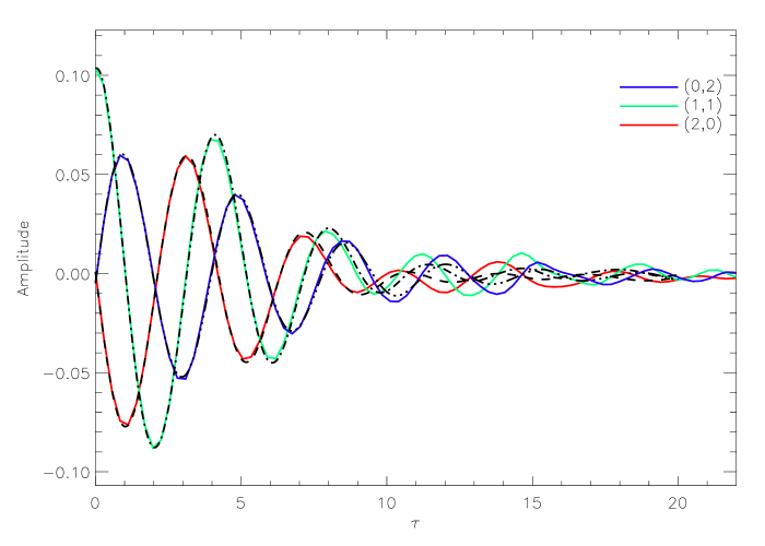
Figure 2: Test-particle coefficient evolutions for an initial ($m=1,n=1$) perturbation with strength $b=0.1$. Time units are the dimensionless time $\tau$ ($\tau\approx 4$ corresponds to one linear oscillation period). The solid lines show the behavior of ensemble average coefficient values from simulations, while the thin broken lines illustrate solutions to the coefficient equation of motion (Equation 34, with Kronecker delta terms omitted in $L$). For clarity, only the evolutions of the three lowest terms are depicted.

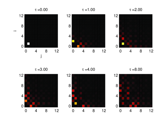
Figure 3: A time sequence of test-particle coefficient strengths resulting from an initial ($m=1,n=1$) perturbation with strength $b=0.1$. Each frame is labeled with the dimensionless time unit corresponding to that snapshot. The shading of the squares represents the relative values of $|c_{m,n}|$, with lighter shades for larger amplitudes. This sequence highlights the phase mixing behavior of the coefficients, in particular, how amplitudes of lower-order terms disperse to higher-order terms.

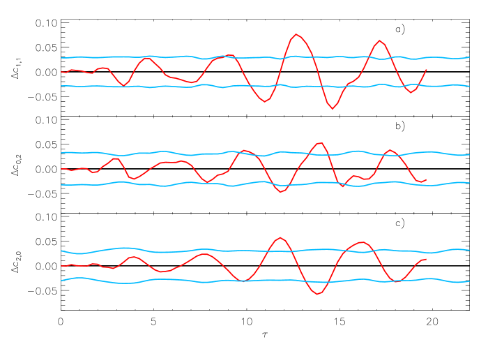
Figure 4: Differences between observed and predicted test-particle coefficient evolutions for an initial ($m=1,n=1$) perturbation with strength $b=0.1$. Each panel shows how an ensemble-averaged coefficient value from simulations $\left<c_{m,n}\right>$ compares to the prediction from Equation 34: $c_{1,1}$ values are in panel a, $c_{0,2}$ in panel b, $c_{2,0}$ in panel c. Difference values shown here are scaled by the initial value of the coefficient of the perturbing term. The horizontal lines represent the “error in the mean” range for ensemble averages.

Figure 5 shows the early evolution of a few low-order coefficients for a self-gravitating system. As in the test-particle case, the (1,1) term is initially perturbed and the line styles are the same as in Figure 2. The overall behavior is strikingly similar to that of the test-particle case. The difference between the coefficient evolution equation and the $N$-body simulations is shown in Figure 6 for $c_{1,1}(0)=0.1$. Figure 7 compares the time behavior of $c_{1,1}$ calculated from Equation 34 for both the test-particle and linear self-gravitating cases. Also shown is the corresponding self-gravitating $N$-body simulation for $c_{1,1}(0)=0.1$. As predicted by the analysis of the $2\times 2$ system, the oscillation period of the linear self-gravitating curve is longer than that of the test-particles curve, and agrees with the $N$-body simulation.

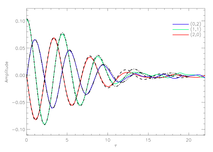
Figure 5: Coefficient evolutions for linear self-gravitation with an initial (1,1) perturbation with strength $b=0.1$. The solid lines show the behavior of ensemble average coefficient values from self-gravitating simulations, while the thin broken lines illustrate solutions to the linear coefficient dynamics relationship (Equation 34, with Kronecker delta terms included). For clarity, only the evolutions of the three lowest terms are depicted.

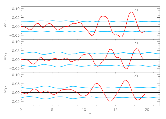
Figure 6: Differences between observed and predicted linear perturbation coefficient evolutions for an initial (1,1) perturbation with strength $b=0.1$. Each panel shows how an ensemble-averaged coefficient value from self-gravitating simulations $\left<c_{m,n}\right>$ compares to the prediction from Equation 34: $c_{1,1}$ values are in panel a, $c_{0,2}$ in panel b, $c_{2,0}$ in panel c. Difference values shown here are scaled by the initial value of the coefficient of the perturbing term. The horizontal lines represent the “error in the mean” range for ensemble averages.

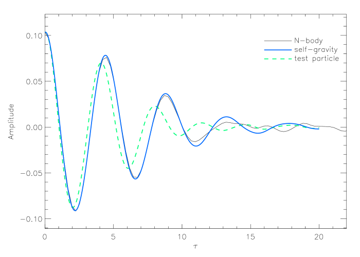
Figure 7: Comparison of test-particle (thick dashed line), linear self-gravitating (thick solid line), and $N$-body simulation (thin solid line) coefficient evolutions for a model with $c_{1,1}(0)=0.1$. The frequency of the linear analysis agrees with the $N$-body simulation. As predicted by the simple system analyzed in Section 5, this frequency is less than the test-particle frequency.

We have also constructed systems with initial (0,2) and (2,0) perturbations for comparison. Figure 8 highlights the fact that (0,2) linear perturbations lead to time-independent solutions, as the initial amplitude in the (0,2) term decreases to a non-zero value as the (2,0) amplitude grows to a non-zero value [similar results develop given an initial (2,0) perturbation]. This behavior is reminiscent of the results of the simple coefficient system developed in Section 5.

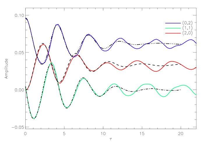
Figure 8: Linear perturbation coefficient evolutions for an initial (0,2) perturbation with strength $b=0.1$. The line styles are the same as in Figure 5. The significant difference between these two figures is that the presence of a time-independent solution is evident as the (0,2) and (2,0) coefficients approach constant, non-zero values with increasing time.

As is evident in Figures 4 and 6, differences between $\left<c_{m,n}\right>$ and $c_{m,n}$ grow with time in both test-particle and self-gravitating cases. To test whether this difference is due to the truncation of the polynomial expansion, we have also solved the equations on a grid where $m_{\rm max}$ and $n_{\rm max}$ are twice the values used to calculate the curves in the figures above. The rms differences between the two $c_{m,n}$ are an order of magnitude smaller than the differences between $\left<c_{m,n}\right>$ and $c_{m,n}$ , so the root cause of the $N$-body/coefficient dynamics discrepancy lies in $N$. As the number of particles in a simulation is increased from $N=1024$ to $N=2048$, the differences between $\left<c_{m,n}\right>$ and $c_{m,n}$ diminish. We have created two self-gravitating ensembles with initial (1,1) perturbations and $b=0.1$. One ensemble is formed from realizations using $N=1024$ particles, the other uses $N=2048$. We have calculated the ratios between the rms $N$-body/coefficient dynamics differences and the error in the mean values for the ensemble. For the $N=1024$ ensemble, these ratios are 1.08, 0.70, and 0.89 for the (1,1), (0,2), and (2,0) terms, respectively. For the $N=2048$ ensemble, the error in the mean values decrease by $\sqrt{2}$, but the rms $N$-body/coefficient dynamics differences decrease by a larger factor, producing ratios of 0.97, 0.66, and 0.83 for the (1,1), (0,2), and (2,0) terms, respectively. We interpret these results to mean that the coefficient dynamics solutions represent the truly collisionless behavior of the system for small enough perturbations, which the $N$-body simulations can only produce in the limit $N\rightarrow\infty$.

In addition to the finite $N$ effects described above, $N$-body simulations always contain some degree of non-linearity that is not included in first-order perturbation theory. We have investigated the effects of non-linearity by tracking ensemble coefficient evolutions as perturbation strengths is increased. Specifically, $N=1024$ particle evolutions with initial (0,2), (1,1), and (2,0) perturbations have been performed, each with strengths $b=0.1$, $b=0.2$, and $b=0.3$. Table 1 quantifies the impact of perturbation strength. As one would expect, the growth of the difference ratios indicates the increased presence of non-linear effects in the $N$-body simulations. Depending on a particular tolerance for discrepancies, one could set a limit on the maximum perturbation strength allowable for an evolution to remain in the linear regime.

Table 1: Ratio of the average rms difference of coefficients, $c_{m,n}$, calculated from Equation 34 and the ensemble values $\left<c_{m,n}\right>$ of the nonlinear $N$-body simulations to the error in the mean of $\left<c_{m,n}\right>$. Each horizontal row has a different initially perturbed polynomial, and each column lists this ratio for a different $c_{m,n}$ for different perturbation strength $b$.

	$c_{0,2}$ ratio			$c_{1,1}$ ratio			$c_{2,0}$ ratio
initial term	$b=0.1$	$b=0.2$	$b=0.3$	$b=0.1$	$b=0.2$	$b=0.3$	$b=0.1$	$b=0.2$	$b=0.3$
$c_{0,2}$	0.75	1.63	3.55	1.14	1.69	3.86	1.02	1.70	3.89
$c_{1,1}$	0.70	1.02	2.04	1.08	1.30	1.90	0.89	1.18	1.73
$c_{2,0}$	1.10	2.21	4.54	1.89	3.75	7.38	1.59	3.13	6.28

7 Discussion

We have demonstrated that a set of orthonormal polynomial terms based on the equilibrium distribution function is useful for investigating the evolution of one-dimensional, self-gravitating, collisionless systems, at least for small linear perturbations from equilibrium. The polynomial coefficients interact via diagonal-neighbor couplings, producing an alternate view of the evolution of these systems in terms of coefficients $c_{m,n}$ on the $(m,n)$ grid.

From a simple “wall clock” point-of-view, a coefficient evolution takes less time to perform than an ensemble calculation. For example, our midpoint method solution (with the timestep discussed in Section 6) on an $m_{\rm max}=60$, $n_{\rm max}=60$ grid takes approximately twenty minutes to evolve to $\tau=30$ on a 3GHz microprocessor using a translator language like MatLab or IDL. On the same machine, each equivalent self-gravitating $N=1024$ realization of an ensemble takes approximately three minutes to evolve with efficient compiled Fortran code. The 100 realization ensembles discussed in this work would have taken five hours to complete, if run serially. The computation time dramatically increases for larger particle numbers, mainly because of the shorter crossing times in the heap-sort algorithm. Each $N=2048$ realization takes approximately eight times as long as the $N=1024$ version. Beyond the time issue, the coefficient evolution approach allows one to follow the behavior of a perfectly smooth distribution function, instead of using density histograms as one must do in the $N$-body approach.

Having said that, coefficient evolutions exhibit their own shortcomings. The size of the $c_{m,n}$ grid that is used determines the resolution of the features of $(x,v)$ phase that can be represented. While we have not developed an analytical relationship between resolution scale and boundary size, there is a conceptual connection that is useful. If one thinks of the Hermite polynomials used to describe velocity behavior, there are $m_{\rm max}$ roots for the $H_{m_{max}}(\varpi)$ term. Phase-space features that have velocity scales smaller than the spacing between the roots will not be properly captured by terms with $m<m_{\rm max}$ and go unresolved by the coefficient dynamics approach. A similar argument may be made for the position aspect of any phase-space feature. For any given situation, one must make a decision regarding an acceptable level of phase-space resolution and then choose $m_{\rm max},n_{\rm max}$ appropriately, a familiar situation when dealing with classical phase-space (Landau & Lifshitz, 1951).

For a constant, uniform time-step, the stability of the midpoint method places a rather severe requirement on the size of $d\tau$. Instabilities occur in the coefficients at large $m$ and $n$ where the derivatives are largest. We have found that $d\tau\lesssim(10\sqrt{m_{max}}n_{max})^{-1}$ for the stability of the midpoint method. As a result, the number of calculations required for an $n_{max}\times n_{max}$ grid scales like $n_{max}^{7/2}$. In principle, one could use different time steps for different regions of phase space, but we did not explore this strategy, since the savings would be modest.

The biggest shortcoming of our approach, however, is the fact that boundary conditions of the grid limit the time that Equation 34 can be used to accurately calculate low-order coefficients so that they can be considered effectively those of an unbounded system. The simple “fixed” boundary conditions we have used, where $c_{m_{max},n}=c_{m,n_{max}}=0$, reflect coefficient amplitude “waves” incident on the boundary back into the interior, where they propagate back toward the low-order coefficients near $(0,0)$. The effect of this reflection at long times on the evolution $c_{2,2}$ is clearly evident in Figure 9.

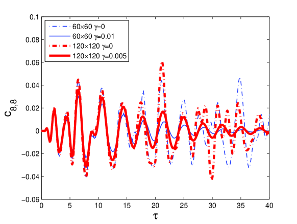
Figure 9: Evolution of $c_{8,8}$ given an initial $c_{1,1}$ perturbation, highlighting boundary effects and damping. The dot-dashed curves represent non-damped solutions defined on different fixed-boundary grids; thin – $60\times 60$ grid and thick – $120\times 120$. The two agree up to $\tau\approx 20$ where reflection from the grid boundary starts to affect the $60\times 60$ curve. Also shown are a damped ($\gamma=1/100$) solution on a $60\times 60$ grid (thin solid curve), and a damped ($\gamma=1/200$) solution on a $120\times 120$ grid (thick solid curve). This form of damping causes the distribution function to decay before it reaches the boundaries, but affects low-order coefficients minimally.

To test the impact of the reflection on the coefficient evolution we have compared two grids, one with twice the dimensions of the other. While a strict quantitative measure is difficult, our investigations suggest that terms with $m,n\lesssim 10$ calculated on an $m_{\rm max}=n_{\rm max}=60$ grid are in good agreement with the same terms calculated on an $m_{\rm max}=n_{\rm max}=120$ grid for $\tau\lesssim 20$. Terms with smaller $m,n$ values show the best agreement between the two grid evolutions. It must also be remembered that only a finite range of $m,n$ terms can be accurately tracked during an $N$-body evolution. For the $N$-values adopted in this work, we have found that, even with ensemble averaging, the particle noise level is comparable to the amplitude of $m,n\gtrsim 10$ terms that arise. While it may be possible to design non-reflecting boundaries (as one would do for the ordinary wave equation), we have not been able to find a scheme that is stable and provides significant improvement over fixed boundary conditions.

Another strategy that shows promise is to include a damping term in the evolution equations. Instead of simply propagating toward large $(m,n)$, disturbances also decay so that the boundaries of the grid are never reached, avoiding distortions due to reflection. Several varieties of damping term have been tested, and the most appealing has the form,

$$\dot{c}_{m,n}^{damping} = -\gamma\left(|L_{m,n}^{m-1,n-1}|+|L_{m,n}^{m+1,n-1}|+\right.$$ (41)

$$\left.|L_{m,n}^{m-1,n+1}|+|L_{m,n}^{m+1,n+1}|\right)c_{m,n},$$

where $1/\gamma$ can be interpreted as a quality factor for the coefficient dynamics. This form has the advantage that the damping rate is proportional to the derivatives of the coefficients, and, other than a gradual decay of the disturbance, its impact on the dynamics of low-order coefficients seems to be minimal. In particular, the oscillation frequencies are hardly affected, for small damping. Figure 9 shows the time-behavior of the $c_{8,8}$ amplitude calculated with two different damping factors. In contrast to the effects of boundary reflections, which lead to complicated distortions throughout the ($m,n$) grid, the effect of damping seems to be a simpler filtering of the amplitude. However, even with this simple form of damping it is not easy to obtain a formula for the region of validity of a coefficient evolution for a given $\tau$. The simplest approach is to pick a grid size and then find the minimum $\gamma$ that keeps the perturbation from reaching the boundaries. Figure 10 shows a reconstructed phase space plot for $m_{max}=n_{max}=120$ with a quality factor $1/\gamma=200$.

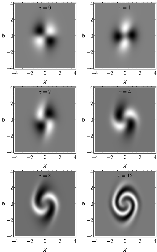
Figure 10: Phase-space evolution of an initial (1,1) perturbation in a self-gravitating system, created from evolving coefficients according to Equation 34 and reconstructing the phase-space distribution function from Equation 13. The coefficient evolution uses a $120\times 120$ grid, with a damping factor $1/\gamma=200$ to eliminate distortions of higher modes.

Regardless of the numerical technique adopted, this polynomial expansion analysis of the Vlasov equation provides a novel, and useful, view of the behavior of one-dimensional self-gravitating systems. While not in the scope of this introductory work, one can imagine several directions any future investigations using this analysis might take. For example one might study the aftermath of the interactions of multiple isolated systems, investigating collisionless processes in the non-equilibrium remnant. Additionally, determining the stationary states of one-dimensional systems or the frequency spectrum of the $L$ matrix could also be approached. One could extend the analysis to second-order to investigate the onset of nonlinear effects, like stability or chaotic behavior. The nearest-neighbor coupling of the coefficients leads to “local” continuity-type dynamics of conserved quantities like energy and fine-grained entropy on the $(m,n)$ grid that should give further insight into the non-equilibrium thermodynamics of these systems.

References

- Alard & Colombi (2005) Alard C., Colombi S., 2005, MNRAS, 359, 123
- Alvord & Miller (2009) Alvord J., Miller B.N., 2009, in Joint Fall 2009 Meeting of the Texas Sections of the APS, AAPT, and SPS. American Phys. Soc., p. C5.002
- Barré et al. (2011) Barré J., Olivetti A., Yamaguchi Y.Y., 2011, J. Phys. A, 44, 405502
- Benhaiem et al. (2013) Benhaiem D., Joyce M., Sicard F., 2013, MNRAS, 429, 3423
- Binney & Tremaine (1987) Binney J., Tremaine S., 1987, Galactic Dynamics. Princeton Univ. Press, Princeton, NJ
- Camm (1950) Camm G.L., 1950, MNRAS, 110, 305
- Cheng & Knorr (1976) Cheng C.Z., Knorr G., 1976, J. Comput. Phys., 22, 330
- Clowe et al. (2006) Clowe D., Bradac M., Gonzalez A.H., Markevitch M., Randall S.W., Jones C., Zaritsky D., 2006, ApJ, 648, L109
- De Packh (1962) De Packh D.C., 1962, J. Electr. Contr., 13, 417
- Fujiwara (1981) Fujiwara T., 1981, PASJ, 33, 513
- Hansen & Moore (2006) Hansen S.H., Moore B., 2006, New Ast., 11, 333
- Hittinger & Banks (2013) Hittinger J.A.F., Banks J.W., 2013, J. Comput. Phys., 241, 118
- Hohl & Feix (1967) Hohl F., Feix M.R., 1967, ApJ, 147, 1164
- Joyce & Worrakitpoonpon (2011) Joyce M., Worrakitpoonpon T., 2011, Phys. Rev. E, 84, 1139
- Kalnajs (1977) Kalnajs A., 1977, ApJ, 212, 637
- Koyama & Konishi (2001) Koyama H., Konishi T., 2001, Phys. Lett. A, 279, 226
- Landau & Lifshitz (1951) Landau L.D., Lifshitz E.M., 1951, Statistical Physics – Part 1. Butterworth-Heinemann, Boston, MA
- Lithwick & Dalal (2011) Lithwick Y., Dalal N, 2011, ApJ, 734, 100
- Mathur (1990) Mathur S., 1990, MNRAS, 243, 529
- Merritt & Aguilar (1985) Merritt D., Aguilar L.A., 1985, MNRAS, 217, 787
- Miller et al. (2007) Miller B.N., Rouet J., Le Guirriec E., 2007, Phys. Rev. E, 76, 6705
- Mohr et al. (1995) Mohr J.J., Evrard A.E., Fabricant D.G., Geller M.J., 1995, ApJ, 447, 8
- Navarro et al. (1996) Navarro J.F., Frenk C.S., White S.D.M., 1996, ApJ, 462, 563
- Navarro et al. (1997) Navarro J.F., Frenk C.S., White S.D.M., 1997, ApJ, 490, 493
- Navarro et al. (2004) Navarro J.F. et al., 2004, MNRAS, 349, 1039
- Nishida et al. (1981) Nishida M.T., Yoshizawa M., Watanabe Y., Inagaki S., Kato S., 1981, PASJ, 33, 567
- Noullez et al. (2003) Noullez A., Aurell E., Fanelli D., 2003, J. Comp. Phys., 186, 697
- Reidl & Miller (1987) Reidl, Jr., C.J., Miller B.N., 1987, ApJ, 318, 248
- Reidl & Miller (1988) Reidl, Jr., C.J., Miller B.N., 1988, ApJ, 332, 619
- Rocha Filho (2013) Rocha Filho T.M., 2013, Computer Physics Communications, 184, 34
- Romanowsky et al. (2003) Romanowsky A.J., Douglas N.G., Arnaboldi M., Kuijken K., Merrifield M.R., Napolitano N.R., Capaccioli M., Freeman K.C., 2003, Science, 301, 1696
- Rubin & Ford (1970) Rubin V.C, Ford W.K., 1970, ApJ, 159, 379
- Rybicki (1971) Rybicki G.B., 1971, Ap&SS, 14, 56
- Schulz et al. (2013) Schulz A.E., Dehnen W., Jungman G., Tremaine S., 2013, MNRAS, 431, 49
- Spergel et al. (2003) Spergel D.N. et al., 2003, ApJS, 148, 175
- Springel et al. (2005) Springel V. et al., 2005, Nature, 435, 629
- Taylor & Navarro (2001) Taylor J., Navarro J., 2001, ApJ, 563, 483
- Valgeas (2006) Valageas P., 2006, A&A, 450, 445
- Watanabe et al. (1981) Watanabe Y., Inagaki S., Nishida M.T., Tanaka Y.D., Kato S., 1981, PASJ, 33, 541
- Weinberg (1991) Weinberg M.D., 1991, ApJ, 373, 391
- Williams & Saha (2011) Williams L.L.R, Saha P., 2011, MNRAS, 415, 448
- Yano & Gouda (1998) Yano T., Gouda N., 1998, ApJS, 118, 267
- Zwicky (1937) Zwicky F., 1937, ApJ, 86, 217