Modeling self-organization of nano-size vacancy clusters
in stochastic systems subjected to irradiation

Abstract

A study of the self-organization of vacancy clusters in irradiated materials is presented. Using a continuum stochastic model we take into account dynamics of point defects and their sinks with elastic interactions of vacancies. Dynamics of vacancy clusters formation is studied analytically and numerically under conditions related to irradiation in both reactors and accelerators. We have shown a difference in patterning dynamics and studied the external noise influence related to fluctuation in a defect production rate. Applying our approach to pure nickel irradiated under different conditions we have shown that vacancy clusters having a linear size $\simeq 6~{}nm$ can arrange in statistical periodic structure with nano-meter range. We have found that linear size of vacancy clusters at accelerator conditions decreases down to $20\%$, whereas a period of vacancy clusters reduces to $6.5\%$.

I Introduction

Metals and alloys under laser and particle irradiation are typical examples of nonequilibrium systems manifesting self-organization processes of point defects with nano-size patterns forming a corresponding microstructure. It is well known that depending on irradiation conditions (displacement damage rate and temperature) point defects can arrange into objects of higher dimension like clusters (di-, tri-, tetra-vacancy clusters), defect walls with vacancy and interstitial loops 118 ; 1110 , voids 111 , precipitates 117 , bubble lattices 114 ; 115 ; 116 . Patterns with spatial structures of nano-meter size can be observed as in a bulk as on a surface of irradiated materials, for example, at ion-beam sputtering CB95 ; MB2004 ; PRE2010 ; CMP2011 ; MetFiz2013 , condensation from gaseous phase PhysScr2012 ; PRE2012 and molecular beam epitaxy PhysScr2011 ; EPJB2013 . Theoretical and experimental investigations of such dissipative structures are widely discussed in literature Martin ; 116 ; 1112 ; Ryazanov ; AbromeitMartin1999 ; Sugakov95 . Numerical studies of defect clusters formation allow one to set up conditions for different kind of patterns emerging in diffusion processes and in processes of defects interaction EPJB2012 ; CMP2013 . A production of defects and the resulting microstructure can principally modify the physical and mechanical properties of an irradiated material leading to swelling, hardening and embrittlement BF2004 ; DKK2009 ; Hardening ; Osetsky ; Gavini . Therefore, from practical and theoretical viewpoints a study of microstructure of material, defects and their arrangement into clusters is a quite urgent problem in modern material science and statistical physics.

According to the standard theory of defects production (see Refs.Walgraef93 ; Walgraef95 ; Walgraef ; Walgraef03 ; mirz1 ) a formation of point defects is of thermo-fluctuation character; the probability of such processes grows with temperature and irradiation flux. It can be realized also at large defects density due to activation barrier height change for defect formation related to elastic deformation of the medium caused by defects presence. It is known that the thermo-fluctuation mechanism for defects generation plays a central role in a structural disorder formation. In this case a concentration of defects exceeds their equilibrium concentration by several orders (concentration of nonequilibrium vacancies is $\simeq 10^{17}\div 10^{20}~{}cm^{-3}$). These defects can migrate in solid, annihilate, collapse into loops or interact with other defects forming spatial dissipative structures. The last one is possible beyond some threshold defined by material properties and irradiation conditions. In such a case a uniform distribution of defects becomes unstable due to their self-organization. As far as a formation of organized defect clusters requires the production of defects in cascades the corresponding microstructure was observed under neutron or ion irradiation. Experimentally (see, for example Ref.JES ) it was shown that under $3MeV$ protons irradiation at low doses ($\simeq 0.01~{}dpa$) a distribution of stacking fault tetrahedrons in $Ni$ and $Cu$ is homogeneous, whereas at elevated doses ($\simeq 0.1~{}dpa$) fluctuations of point defect clusters were observed. At doses up to $0.65~{}dpa$ one gets well periodic structure of defect clusters. Moreover, as was shown in Ref.Kiritani90 vacancy clusters in the form of stacking fault tetrahedra can be formed from collision cascades at low temperatures when vacancies do not make their motion by thermal activation. Formation of stacking fault tetrahedron was experimentally observed even under electron irradiation of foils Kiritani78 ; Kiritani00 ; SYMK2004 . It was shown that vacancy clusters in electron irradiated metals, appear under the circumstances of local enrichment of vacancies as the result of the behavior of interstitials atoms. In experimental studies vacancy clusters have linear size on several nano-meters (in the interval $2\div 7~{}nm$ depending on irradiation conditions and used material target) with $7\div 20$ vacancies inside clusters SYMK2004 .

Understanding of the defect population dynamics and microstructure transformations is thus of fundamental importance, not for its intrinsic interest, but also for its technological significance. It allows one to describe macroscopic ordering processes, phase separation in solids under different conditions of external influence Mazias ; Kiritani ; EnriqueBellon00 ; Enrique63 ; YeBellon04_1 . Despite the main mechanisms of radiation damage in solids are known Kiritani91 nowadays multiscale approaches treating the system under consideration at different hierarchical levels (from atomic to mesoscopic level) are used to study microstructure transformation in irradiated materials MLN ; NIMB2001 ; MMS04 . On a mesoscopic level such processes can be studied within the framework of a rate theory where concentrations/densities of main structural elements (defects, their clusters, sinks) are considered Martin ; AbromeitMartin1999 ; 1112 . Usually such models take into account defects production rate, their annihilation and diffusion of mobile species (vacancies and interstitials) Walgraef95 ; Walgraef . Unfortunately, a generation of defects caused by elastic deformation of the medium and their interactions caused by “chemical” forces are not considered as usual. Moreover, as far as irradiation occurs at elevated temperatures (depending on the irradiation conditions, namely, dose rate $K\sim 10^{-6}\div 10^{-3}~{}dpa/sec$ and temperature $T\sim 500\div 1000~{}K$) fluctuations of defects production lead to stochastic dynamics of defect populations. Properties of stochastic defects production in irradiated materials and stochastic formation of stacking fault tetrahedrons (vacancy clusters) were discussed in Refs.Kiritani ; Kiritani_MCF97 . A stochastic production of defects during irradiation influence was proposed in Ref.Yanovski , where it was assumed that the corresponding stochastic athermal mixing of atoms caused by irradiation can be described as spatially correlated random process giving the effective flux opposite to the diffusion one. This idea was exploited studying ordering, patterning and phase separation in irradiated materials EPJB2010 ; PhysA2010_1 ; CEJP2011 ; UJP2012 . In such a case the corresponding fluctuations are caused by an external influence (energy dispersion of particles in irradiation flux, dispersion in an incidence angle, etc.) and are considered as an external noise. From the other hand in systems with birth-and-death processes or “chemical reactions” (production of defects and their annihilation) and diffusion there is another kind of fluctuation source relevant to internal nature of the system. The corresponding internal noise is defined by a heat bath. Its influence on arrangement of ensemble of vacancies was studied theoretically in Refs.EPJB2012 ; CMP2013 ; UJP2013 , where it was shown that depending on internal noise properties different kinds of vacancy structures emerge.

From both theoretical and practical viewpoints it is important that dynamics of defects and, therefore, the corresponding microstructure are quite different at conditions relevant to irradiation in reactors ($K=10^{-6}~{}dpa/sec$, $T=773~{}K$) and in accelerators ($K=10^{-3}~{}dpa/sec$, $T=900~{}K$). Under reactor conditions the principal role belongs to diffusion processes, whereas irradiation in accelerators gives high damage rates with small contribution of diffusion processes. It results in different spatial arrangement of defects in these two cases. Therefore, the studying different physical processes of defects arrangement in irradiated materials under different irradiation conditions is actual. In this paper we are aimed to study dynamics of defects at their self-organization under reactor and accelerator conditions considering behavior of point defects and their sinks. Using the approach proposed in Ref.Walgraef95 we take into account defects production caused by local elastic deformation of material and stochastic effects induced by external noise influence. In our study pure $Ni$ (as most wide-spread constructional material in atomic energy) was selected as a reference system. We will show that the external noise influence can be different in the case of irradiation under reactor and accelerator conditions. In the first case it promotes large difference in vacancy clusters occupation numbers comparing to the second case. Moreover, it is able to reduce the linear size of vacancy clusters and a period of their arrangement. It will be shown that both linear size of vacancy clusters and their period are of several nano-meter range.

The paper is organized as follows. In Section II we present a generalized model describing the main mechanisms of defects formation with two spatial scales related to diffusion scale and defects interaction scale. In Section III we consider a reduced one-component model analytically assuming constant sink densities. Here we find critical values for both defect damage rate and temperature limiting the patterning in the system. Section IV is devoted to study a general model for pattern formation in system of defects numerically. Here we discuss the difference in defects arrangement under reactor and accelerator conditions. We conclude in Section V.

II Model

In the framework of the rate theory evolution equations for populations of vacancies $c_{v}$ and interstitials $c_{i}$ are of the form Walgraef95 ; Walgraef :

$$\begin{split}&\partial_{t}c_{i}=K(1-\varepsilon_{i})-D_{i}S_{i}c_{i}-\alpha c_{i}c_{v},\\ &\partial_{t}c_{v}=K(1-\varepsilon_{v})-D_{v}S_{v}(c_{v}-c_{0v})-\alpha c_{i}c_{v}.\end{split}$$ (1)

Here the equilibrium vacancy concentration $c_{0v}=e^{-E^{f}_{v}/T}$ is defined through vacancy formation energy $E^{f}_{v}$ and temperature $T$; $K$ is the defect damage rate; $\varepsilon_{i}$ and $\varepsilon_{v}$ relate to cascades collapse efficiency ($\varepsilon_{v}\gg\varepsilon_{i}$); $D_{v,i}=D^{0}_{v,i}e^{-E^{m}_{v,i}/T}$ are diffusivities defined through the migration energies $E^{m}_{v,i}$. Sink intensities $S_{i}\equiv Z_{iN}\rho_{N}+Z_{iV}\rho_{v}+Z_{iI}\rho_{i}$ and $S_{v}\equiv Z_{vN}\rho_{N}+Z_{vV}\rho_{v}+Z_{vI}\rho_{i}$ are determined by the network dislocation density $\rho_{N}$ and densities of vacancy and interstitial loops $\rho_{v,i}$ with preference $Z_{\{\cdot,\cdot\}\cdot}$ where $Z_{vN}=Z_{vI}=Z_{vV}=1$, $Z_{iN}=1+B$, $Z_{iI}\simeq Z_{iV}\simeq 1+B^{{}^{\prime}}$; $B$ and $B^{{}^{\prime}}\geq B$ are excesses for network bias and loop bias ($B\simeq 0.1$). The recombination coefficient $\alpha={4\pi r_{0}(D_{i}+D_{v})}/{\Omega}$ is defined through the interaction radius of defects $r_{0}$, the atomic volume $\Omega$ and the corresponding diffusivities. Evolution equations for the loop densities are as follows Walgraef95 ; Walgraef :

$$\begin{split}&\partial_{t}\rho_{i}=\frac{2\pi N}{b}\left(\varepsilon_{i}K+D_{i}Z_{iI}c_{i}-D_{v}Z_{vI}(c_{v}-c_{v0})\right);\\ &\partial_{t}\rho_{v}=\frac{1}{br^{0}_{v}}\left(\varepsilon_{v}K-\rho_{v}[D_{i}Z_{iV}c_{i}-D_{v}Z_{vV}(c_{v}-c_{v0})]\right).\end{split}$$ (2)

Here $\vec{b}$ is the Burgers vector with modulus $b\equiv|\vec{b}|$, $r^{0}_{v}$ is the initial vacancy loop radius, $N$ is the sinks density.

Using renormalized quantities $\rho^{\prime}_{v,i}\equiv\rho_{v,i}/\rho_{N}$, $t^{{}^{\prime}}\equiv t\lambda_{v}$, $\lambda_{v}\equiv D_{v}Z_{vN}\rho_{N}$, $x_{i,v}=\gamma c_{i,v}$, $\gamma\equiv\alpha/\lambda_{v}$, $P\equiv\gamma K/\lambda_{v}$, $\mu\equiv(1+\rho^{\prime}_{v}+\rho^{\prime}_{i})$, $Z_{iN}/Z_{vN}=1+B$ and introducing small parameter $\epsilon\equiv D_{v}/D_{i}\ll 1$ one can eliminate population of interstitials adiabatically taking $\epsilon\partial_{t}x_{i}\simeq 0$. It gives $x_{i}={{P}(1-\varepsilon_{i})}/[(1+B)\mu/{\epsilon}+x_{v}]$. In such a case we arrive at the system of three equations: one for the vacancy population $x\equiv x_{v}$ and two others for loop densities; next we drop primes.

It should be noted that a formation of point defects is of thermo-fluctuating character and the corresponding probability increases with a growth in the temperature, irradiation or defects density mirz1 . As was shown in Ref.mirz2 physically it relates to a change in the activation barrier for defects formation due to elastic deformation of the medium caused by defects presence. To take into account such effects one can introduce the component relevant to this mechanism in the form: $G\exp(E_{e}(r)/T)$, where the prefactor $G=p\omega_{D}\gamma/\lambda_{v}e^{-(E^{f}_{v}+E^{m}_{v})/T}$ describes probability of this process governed by vacancy formation and migration energies $E^{f}_{v}$ and $E^{m}_{v}$, Debye frequency $\omega_{D}$ and the probability factor $p\ll 1$; $E^{e}(r)$ is the activation energy changing due to elastic field produced by defects. Following Ref.mirz2 , we assume $G\exp(\varepsilon x/(1+x^{2}))$, where $\varepsilon\equiv 2ZE_{e}^{0}/T$ is given by the energy of deformations $E_{e}^{0}$ and coordination number $Z$. Generally this additional term is essential at laser irradiation comparing to defects production in cascades. Next, following Ref.EPJB2012 we retain this term without loss of generality.

From physical viewpoint vacancies are mobile species. Therefore, we have to introduce their flux. Generally, it contains pure diffusion part $-L_{d}^{2}\nabla x$ with diffusion length $L_{d}^{2}\equiv D_{v}/\lambda_{v}$ and the component describing defects interaction $\mathbf{v}x=-(L_{d}^{2}/T)x\nabla U$. For the interaction potential we assume self-consistency relation BHKM97 ; PhysicaD ; MetFiz09 ; EPJB2012 $U=-\int\tilde{u}(r,r^{\prime})x(r^{\prime}){\rm d}r^{\prime}$, where $-\tilde{u}(r)$ is the attraction potential with properties $\int\tilde{u}(r)r^{2n+1}{\rm d}r=0$. Assuming that $x(r)$ does not change essentially on the distance $r_{0}\simeq\Omega^{1/3}$, one can use an expansion

$$\frac{1}{T}\int{\rm d}\mathbf{r}^{\prime}\tilde{u}(\mathbf{r}-\mathbf{r}^{\prime})x(\mathbf{r}^{\prime})\simeq\varepsilon(x+r_{0}^{2}\nabla^{2}x).$$ (3)

Here the first term leads to the well-known relation between the elastic field potential and the defects concentration $U=-\kappa\varpi\nabla\cdot\mathbf{u}$; for the displacement vector $\mathbf{u}$ one has $\nabla\cdot\mathbf{u}\propto\varpi x$, $\kappa$ is the elastic constant, $\varpi$ is the dilatation parameter mirz1 . The second part in Eq.(3) is responsible for microscopic processes of defect interactions in the vicinity of the interaction radius $r_{0}$. Under normal conditions this term is negligible comparing to the ordinary diffusion one. However, in the absence of the second term in Eq.(3) for the flux one gets $\mathbf{J}\propto-(1-\varpi\kappa x/T)\nabla x$, where the the concentration depending diffusion coefficient $(1-\varpi\kappa x/T)$ can be negative at some interval for $x$. It means that homogeneous distribution of defects starting from some critical speed of its formation related to the temperature, sinks density, and dilatation volume becomes unstable. The emergence of the directional flux of defects results in supersaturation of vacancies and formation of clusters or pores. From mathematical viewpoint such divergence appeared at short time scales can not be compensated by nonlinear part of the reaction terms. The second term in expansion (3) can prevent divergencies of the derived model due to microscopic properties of defect interactions. Therefore, the term with the second derivative must be retained. It will be shown that this term governs the typical sizes of defect clusters.

Taking into account all above mechanisms one arrives at the system of dynamical equations of the form

$$\begin{split}\partial_{t}x=&P(1-\varepsilon_{v})-(1+\rho_{i}+\rho_{v})(x-x_{0})\\ &-\frac{P\epsilon(1-\varepsilon_{i})x}{A(1+\rho_{i}+\rho_{v})+{\epsilon}x}+Ge^{\frac{\varepsilon x}{1+x^{2}}}-\nabla\cdot\mathbf{J};\\ \tau_{i}\partial_{t}\rho_{i}&=\varepsilon_{i}P+\frac{\tilde{A}AP(1-\varepsilon_{i})}{A(1+\rho_{i}+\rho_{v})+{\epsilon}x}-(x-x_{0});\\ \tau_{v}\partial_{t}\rho_{v}&=\varepsilon_{v}P-\rho_{v}\left(\frac{\tilde{A}AP(1-\varepsilon_{i})}{A(1+\rho_{i}+\rho_{v})+{\epsilon}x}-(x-x_{0})\right),\end{split}$$ (4)

where the renormalized defect flux is

$$\mathbf{J}\equiv-\left[\nabla x-\varepsilon x\nabla(x+\ell^{2}\nabla^{2}x)\right].$$ (5)

Here we have used renormalization $\mathbf{r}^{\prime}=\mathbf{r}/L_{d}$ and introduced dimensionless length $\ell^{2}=r_{0}^{2}/L_{d}^{2}$ with time scales $\tau_{i}\equiv br_{v}^{0}\rho_{N}\gamma$, $\tau_{v}\equiv b\alpha\rho_{N}/2\pi ND_{v}$; $\Delta B=B-B^{\prime}$, $A\equiv 1+B$, $\tilde{A}\equiv 1+\Delta B$.

The time scale for the vacancy population evolution is several times larger than relaxation of cascades. It means that a particle bombardment occurs every time at new spatially organized system. In other words, the cross-section of defects formation or defect damage rate and/or cascade collapse efficiency generally can be considered as fluctuating parameters Kiritani ; Kiritani_MCF97 . In such a case, formally, one can consider stochastic nature of $P$ assuming $P\to\langle P\rangle+\zeta(\mathbf{r},t)$ where $\zeta(\mathbf{r},t)$ represents corresponding fluctuations with properties $\langle\zeta\rangle=0$ and $\langle\zeta(\mathbf{r},t)\zeta(\mathbf{r}^{\prime},t^{\prime})\rangle=2\sigma^{2}\delta(\mathbf{r}-\mathbf{r}^{\prime},t-t^{\prime})$. Here $\sigma^{2}$ is the noise intensity proportional to $P$ meaning that fluctuating source emerges only if irradiation is included; $\delta$-correlated noise describes fast relaxation of cascades comparing to evolution of the population field. In such a case this term should be included into dynamics of the system (4) where stochastic dynamics we will treat in the Stratonovich calculus. As a reference system we consider pure nickel with following material constants: $E^{f}_{v}=1.8eV$, $E^{m}_{v}=1.04~{}eV$, $E^{m}_{i}=0.3~{}eV$, $E^{e}_{0}=0.01\div 0.2~{}eV$, $D_{v}=6\cdot 10^{-5}e^{-E^{m}_{v}/T}~{}m^{2}/sec$, $D_{i}=10^{-7}e^{-E^{m}_{i}/T}~{}m^{2}/sec$, $c_{0v}=e^{-E^{f}_{v}/T}$, $\omega_{D}=1.11\cdot 10^{13}~{}sec^{-1}$ $r^{0}_{v}=1.5\cdot 10^{-9}~{}m$, $\varepsilon_{v}=0.1$, $\varepsilon_{i}=0.01$, $\rho_{N}=10^{14}~{}m^{-2}$, $\Omega=1.206\cdot 10^{-29}~{}m^{3}$.

III One-component system

Comparing time scales for vacancy and interstitial loop densities with time scale for vacancy population one finds that $\tau_{i}\gg\tau_{v}\gg 1$. It allows one to consider $\rho_{i}$ and $\rho_{v}$ as slow quantities. Hence, we can consider a spatial modulation of the vacancy concentration field assuming $\mu\equiv(1+\rho_{i}+\rho_{v})\approx const$. Therefore, the system (4) can be effectively reduced to the one-component model with the external noise:

$$\partial_{t}x=R_{x}(x)-\nabla\cdot\mathbf{J}+g_{x}(x)\zeta(\mathbf{r},t),$$ (6)

where

$$\begin{split}&R_{x}(x)=P(1-\varepsilon_{v})-\mu(x-x_{0})-\frac{P\epsilon(1-\varepsilon_{i})x}{A\mu+{\epsilon}x}+Ge^{\frac{\varepsilon x}{1+x^{2}}},\\ &g_{x}^{2}(x)=(1-\varepsilon_{v})^{2}+\left(\frac{\epsilon(1-\varepsilon_{i})x}{A\mu+{\epsilon}x}\right)^{2}.\end{split}$$ (7)

Let us consider stability of the stationary homogeneous state $x_{s}$ as a solution of the equation $R_{x}(x)=0$. The corresponding phase diagram in the plane $(K,T)$ and stationary dependencies of vacancy concentration are shown in Fig.1. It follows that due to influence of the elastic field the system manifests bistable regime (cf. curves in insertion at different $p$). In the domains $I$ the system is monostable. The bistability domain $II$ bounded by interval $K\in[K_{b1},K_{b2}]$ shrinks with decrease in $E^{0}_{e}$.

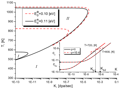
Figure 1: Phase diagram and stationary states of the deterministic system

Considering dynamics of the averaged fluctuation $\langle\delta x\rangle=\langle x\rangle-x_{s}$ in the Fourier space we obtain

$$\frac{{\rm d}\langle\delta x\rangle}{{\rm d}t}=\left(\Lambda+\omega(k)\right)\langle\delta x\rangle,$$ (8)

where the Lyapunov exponent is

$$\begin{split}\Lambda&=-\mu-{\frac{{P}(1-\varepsilon_{i})\epsilon\,\mu\,A}{\left[A\mu+x_{s}\epsilon\right]^{2}}}+G\frac{\varepsilon(1-x_{s}^{2})}{(1+x_{s}^{2})^{2}}\exp\left(\frac{\varepsilon x_{s}}{1+x_{s}^{2}}\right)\\ &+\frac{\sigma^{2}\epsilon^{2}(1-\varepsilon_{i})^{2}}{\left[A\mu+\epsilon x_{s}\right]^{2}}\left(1-\frac{\epsilon x_{s}}{A\mu+\epsilon x_{s}}\left[4-\frac{3\epsilon x_{s}}{A\mu+\epsilon x_{s}}\right]\right).\end{split}$$ (9)

Here the last term represents a contribution from the Stratonovich drift leading to destabilization of the homogeneous state. The noise action leads to destabilization increasing the value of $\Lambda$. A dispersion relation describing instability with respect to inhomogeneous perturbations is given by

$$\omega(k)=-k^{2}[1-\varepsilon x_{s}(1-\ell^{2}k^{2})].$$ (10)

It follows that unstable modes with $\omega(k)>0$ are characterized by wave-numbers $0<k<k_{c}$, where

$$k_{c}=\sqrt{\frac{\varepsilon x_{s}-1}{\varepsilon x_{s}\ell^{2}}}.$$ (11)

It is seen that in the simplest case of $\ell\to 0$ in monostable domain (below the cusp) all states with $x_{s}>1/\varepsilon$ are unstable with respect to inhomogeneous perturbations with $k_{c}\to\infty$, whereas states with $x_{s}<1/\varepsilon$ are stable. In the actual case $\ell\neq 0$ the system states characterized by $x_{s}>1/\varepsilon$ are unstable with wave numbers lying in the interval $0<k<k_{c}$. In the bimodal domain the system is always unstable with respect to inhomogeneous perturbations. The wave number for the most unstable mode $k_{0}$ can be found from the solution of the equation ${\rm d}\omega(k)/{\rm d}k=0$ giving $k_{0}=k_{c}/\sqrt{2}$. Dependencies $\omega(k)$ at different values for $\mu$ are shown in Fig.2 (top panel). An increase in sinks density leads to lower value of $x_{s}$. This results to a stabilization of the uniform defects distribution, as was shown previously in Ref.Walgraef95 : in the studied system the maximal value of $\omega(k)$ decreases resulting to a shift of $k_{c}$ toward small values (see Fig.2 (bottom panel)). Hence, at elevated sink densities a number of unstable modes decreases and period of patterns characterized by most unstable mode $k_{0}$ grows.

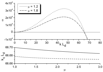
Figure 2: Dispersion law at different sink densities under reactor conditions (top) and dependencies of critical wave number versus sink densities (bottom) under accelerator (solid line) and reactor (dash line) conditions

Next, let us consider the system behavior in the stationary case setting $\ell\lll 1$. It allows one to use mean-field approximation resulting in $\nabla^{2}x\to(x-\eta)$ and $(\nabla x)^{2}\to(x-\eta)^{2}$, where $\eta\equiv\langle x\rangle$ is the mean field (in systems undergoing order-disorder phase transitions it plays a role of the order parameter) describing ordering effects Garcia . The averaging is provided according to stationary distribution function $\mathcal{P}_{s}(t\to\infty;x,\eta)=\mathcal{P}_{s}(x,\eta)$ as solution of the corresponding Fokker-Planck equation Risken :

$$\frac{\partial\mathcal{P}}{\partial t}=-\frac{\partial}{\partial x}\left(R_{x}(x)+(1-\varepsilon x)(x-\eta)-\varepsilon(x-\eta)^{2}\right)\mathcal{P}+\sigma^{2}\frac{\partial}{\partial x}g_{x}(x)\frac{\partial}{\partial x}g_{x}(x)\mathcal{P}.$$ (12)

Its stationary solution

$$\mathcal{P}_{s}(x;\eta)=\frac{1}{\mathcal{N}(\eta)}\exp\left(\frac{1}{\sigma^{2}}\int\limits_{0}^{x}\frac{R_{x}(y)-(1-\varepsilon y)(y-\eta)+\varepsilon(y-\eta)^{2}-\sigma^{2}g_{x}(y)g_{x}^{\prime}(y)}{g_{x}^{2}(y)}{\rm d}y\right)$$ (13)

defines the mean field in a self-consistent manner

$$\eta=\int\limits_{0}^{\infty}x\mathcal{P}_{s}(x;\eta){\rm d}x;$$ (14)

constant $\mathcal{N}(\eta)$ takes care of the normalization condition $\int_{0}^{\infty}\mathcal{P}_{s}(x;\eta){\rm d}x=1$.

Solutions of the self-consistency equation (14) are shown in Fig.3a. It follows that the mean field falls down with the temperature increase meaning a loss of spatial order. Comparing the corresponding curves at different defect damage rates one obtains that spatial organization is larger at elevated $K$ due to formation of new interacting defects. The external noise action does not change principally the dependencies $\eta(K,T)$. Here one has small decrease of the mean field at actual temperature regime relevant to reactors, for example, and small increase in $\eta$ at elevated temperatures. As far as external fluctuations decrease $\eta$ the stationary value of concentration $x_{s}$ (in stochastic case it is reduced to most probable value) decreases too leading to an extension of the number of unstable modes, comparing to the deterministic case (see Eqs.(10,11)). Therefore, the period of pattern described by the wave number $k_{0}$ grows with the noise influence.

Using mean field results one can obtain critical values of $\eta$ limiting supersaturation of point defects above which spatial modulation is realized. Indeed, as far as $\eta$ is a measure of the averaged point defects population $\eta\equiv\langle x\rangle$ we can define the supersaturation in the standard manner $\Delta\equiv(\eta-x_{0})/x_{0}$, where $\Delta=\Delta(K,T)$, $x_{0}$ relates to the equilibrium vacancy population. Next, choosing a value of $K$ we can obtain the critical value of the temperature from the phase diagram obtained from the linear stability analysis (follow the arrow in Fig.3a). This is the maximal temperature $T_{max}$ bounding the temperature domain $(T<T_{max})$ for spatial instability, whereas $K_{min}$ is the minimal damage rate $(K>K_{min})$ bounding spatial instability. The critical value $\eta_{c}$ we define as $\eta_{c}=\eta(K_{min},T_{max})$. Therefore, we arrive at the dependence of the critical supersaturation $\Delta_{c}(K,T)$ of point defects limiting spatial organization of defect structure (see Fig.3b). It follows that $\Delta_{c}$ decreases with growth of both $K$ and $T$ meaning emergence of ordering/patterning processes at low population of point defects at elevated $K$ or $T$. The physical reason for this effect lies in production of large amount of defects by irradiation and their generation by the thermo-activation mechanism.

a)
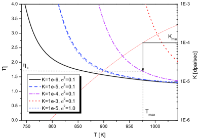
b)

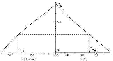
Figure 3: Mean field results: a) mean field dependence on the temperature at different defect damage rates and the external noise intensity (a procedure to determine critical value $\eta_{c}$ is shown by arrows with the help of the linear stability diagram in the plane $(T,K)$); b) two-dimensional plot of the critical supersaturation dependence $\Delta_{c}\equiv\Delta_{c}(K,T)=(\eta_{c}(K,T)-x_{0}(T))/x_{0}(T)$ at $\sigma^{2}=0.1$

IV Three-component system

In the three-component stochastic model we take $\rho_{i,v}=\rho_{i,v}(t)$, giving $\mu=\mu(t)$. Therefore, instead of the deterministic system (4) we arrive at

$$\begin{split}\partial_{t}x&=R_{x}(x;\rho_{i},\rho_{v})-\nabla\cdot\mathbf{J}+g_{x}(x;\rho_{i},\rho_{v})\zeta(\mathbf{r},t);\\ \tau_{i}\partial_{t}\rho_{i}&=R_{i}(\rho_{i};x,\rho_{v})+g_{i}(\rho_{i};x,\rho_{v})\zeta(\mathbf{r},t);\\ \tau_{v}\partial_{t}\rho_{v}&=R_{v}(\rho_{v};x,\rho_{i})+g_{v}(\rho_{v};x,\rho_{i})\zeta(\mathbf{r},t),\end{split}$$ (15)

here $R_{x}$ and $g_{x}$ are given by Eq.(7). For the deterministic components $R_{i}$, $R_{v}$ and noise amplitudes $g_{i}$, $g_{v}$ one has:

$$\begin{split}R_{i}&\equiv\varepsilon_{i}P+\frac{\tilde{A}AP(1-\varepsilon_{i})}{A(1+\rho_{i}+\rho_{v})+{\epsilon}x}-(x-x_{0}),\\ R_{v}&\equiv\varepsilon_{v}P-\rho_{v}\left(\frac{\tilde{A}AP(1-\varepsilon_{i})}{A(1+\rho_{i}+\rho_{v})+{\epsilon}x}-(x-x_{0})\right),\\ g^{2}_{i}&\equiv\varepsilon_{i}^{2}+\left(\frac{\tilde{A}A(1-\varepsilon_{i})}{A(1+\rho_{i}+\rho_{v})+{\epsilon}x}\right)^{2},\\ g^{2}_{v}&\equiv\varepsilon_{v}^{2}+\left(\frac{\tilde{A}A(1-\varepsilon_{i})\rho_{v}}{A(1+\rho_{i}+\rho_{v})+{\epsilon}x}\right)^{2}.\end{split}$$ (16)

In our study we make numerical analysis on 2-dimensional square lattice $N\times N$ where $N=128$ with periodic boundary conditions and mesh size $\Delta l=1.0$. For the numerical integration the Milshtein method was used Garcia . The time step is $\Delta t=2.5\times 10^{-4}$. In all numerical experiments initial conditions correspond to equilibrium concentration of vacancies with no loops, i.e, $\langle c(\mathbf{r},0)\rangle=c_{eq}$, with small dispersion $\langle(\delta c(\mathbf{r},0))^{2}\rangle=10^{-1}c_{eq}$; $\langle\rho_{i}(\mathbf{r},0)\rangle=\langle\rho_{v}(\mathbf{r},0)\rangle=0$. We consider two regimes of irradiation corresponding to reactor and accelerator conditions. In the modeling scheme we put $\ell=0.25$ in order to stabilize the computational algorithm. An estimation for this parameter for pure $Ni$ gives $\ell_{Ni}=0.015$. Hence, in numerical data analysis we will use the renormalization parameter $\chi\equiv\ell_{Ni}/\ell=0.06$ to estimate a linear size of defect clusters $\langle d_{0}\rangle$ and a characteristic length of their spatial distribution $L_{0}$.

IV.1 Patterning under reactor conditions

Let us consider patterning under reactor conditions. Typical snapshots of the system evolution are shown in Fig.4. Here first, second and third columns correspond to dynamics of the dimensionless fields $x(\mathbf{r},t)$, $\rho_{i}(\mathbf{r},t)$ and $\rho_{v}(\mathbf{r},t)$, respectively. It is seen that at early stages of the system evolution starting from the Gaussian distribution of vacancies around the equilibrium value the spatial arrangement of defects is realized. Here small spherical clusters and extended ones representing defect walls are organized (see first column). Their spatial structure is slightly changed at further system evolution. Increasing the irradiation dose $Kt$ one can observe well organized structure of vacancy loops repeating spatial structure of vacancy clusters, whereas interstitial loops density behaves vice verse to the vacancy loops density. Moreover, at early stages one can find smearing of the fields $\rho_{i}$ and $\rho_{v}$ in the vicinity of the extended defects. With the irradiation dose increase the number of loops grows.

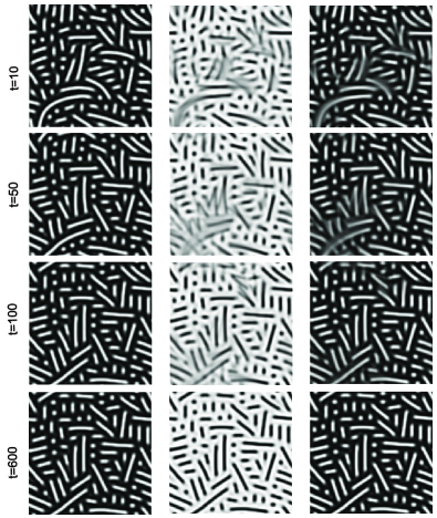
Figure 4: Typical evolution of the deterministic ($\sigma^{2}=0$) system under reactor conditions ($T=773$K, $K=10^{-6}~{}dpa/sec$). Columns (from the left to the right) denote dynamics of fields $x$, $\rho_{i}$, $\rho_{v}$.

To study self-organization of vacancy clusters we consider dynamics of the quantity $\langle(\delta x)^{2}\rangle$. In patterning processes it plays a role of the effective order parameter measuring symmetry breaking of initial Gaussianly distributed field Garcia ; PhysicaD ; PhysA2010_1 . Considering its dynamics together with the averaged concentration $\langle x\rangle$ one finds that at early stages the number of point defects increases toward its maximal value (see Fig.5).

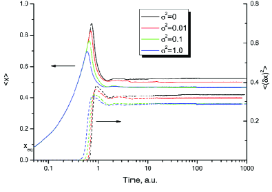
Figure 5: Dynamics of the averaged concentration field and its variance $\langle(\delta x)^{2}\rangle$ at different values for the external noise intensity $\sigma^{2}$ under reactor conditions.

From this time the variance $\langle(\delta x)^{2}\rangle$ grows meaning formation of spatial order. Here due to a supersaturation of vacancies produced by irradiation cascades a vacancy enriched phase (spherical clusters and defect walls) appears. As a result the number of free vacancies decreases due to migration to sinks. An emergence of weak oscillations here corresponds to processes when migrating vacancies can be absorbed by clusters and emitted from them absorbing by sinks. At irradiation dose increase the quantity $\langle x\rangle$ attains the stationary value with small fluctuations. It means that new vacancies formed in cascades move to sinks with small amount in a bulk. Domains having small amount of vacancies contain elevated interstitial loop densities (see second column in Fig.4). Comparing dependencies in Fig.5 at different noise intensities one can conclude that the noise action accelerates formation of spatial order due to instability described by the Stratonovich drift as was shown in the previous Section. From the other hand it reduces the averaged vacancy concentration and a value of the order parameter. The last means small variance of the concentration field in the system at elevated intensity of external fluctuations. In other words another kind of the spatial modulation of vacancy field is realized with small value of the averaged vacancy concentration. Indeed, comparing snapshots for vacancy field distribution at different noise intensities it is seen that external fluctuations promote spatial rearrangement of vacancies with preferable formation of spherical clusters (see Fig.6a). From the obtained histograms of the vacancy cluster size distribution it follows that in the deterministic case there are three well-defined peaks in distributions corresponding to small spherical clusters characterized by areas $s<\langle s\rangle$ and extended clusters with $s\simeq\langle s\rangle$ and $s>\langle s\rangle$. At elevated noise intensity extended clusters can not be formed due to large fluctuations in defects production rate resulting in formation of small clusters. Here the probability density takes large values at $s<\langle s\rangle$; extended clusters have small probability for organization. Moreover, with the noise intensity increase the peak of the corresponding distribution shifts toward $s/\langle s\rangle=1$.

To study the noise influence on a period of patterns we consider a spherically averaged structure function for the vacancy concentration field $S(k,t)=N^{-2}\sum_{k<|\mathbf{k}|<k+\Delta k}S(\mathbf{k},t)$, where $S(\mathbf{k},t)=\langle\delta x_{-\mathbf{k}}\delta x_{\mathbf{k}}\rangle$, $\delta x=x-\langle x\rangle$, $x_{\mathbf{k}}=\int{\rm d}\mathbf{r}x(\mathbf{r},t)e^{i\mathbf{kr}}$. The corresponding dependencies at fixed time are shown in Fig.6b. In the deterministic case the peak of $S(k)$ is smeared due to realization of extended structures. At elevated noise intensities the number of extended structures decreases and we get a narrow peak with higher value for $S(k)$. It is well seen that period of structures decreases slightly due to formation of the large number of spherical vacancy clusters. The area under curves $S(k)$ decreases with the noise intensity growth that well corresponds to lower values of the order parameter $\langle(\delta x)^{2}\rangle$. From the obtained data and diffusion length definition $L_{d}\propto\rho_{N}^{-1/2}\sim 10^{7}~{}m$ one can conclude that the period of vacancy clusters $L_{0}$ related to position of the main peak of the structure function slightly varies in the interval $L_{0}\sim(4.8\div 4.5)\chi L_{d}$ with the noise intensity growth. Estimation for the averaged linear size of vacancy clusters (diameter for spherical objects) $\langle d_{0}\rangle$ gives $\langle d_{0}\rangle\simeq\chi L_{d}\sim 6~{}nm$. Using the obtained data one can study vacancy distribution inside clusters. The corresponding distribution functions $f(x)$ are shown in Fig.6c in both deterministic and stochastic cases. It is seen that most of clusters are characterized by concentration less that mean value $\langle x\rangle$, however, there is well defined peak related to vacancy clusters with concentration $x>\langle x\rangle$. The external fluctuations increase vacancy concentration in clusters shifting two main peaks of $f(x)$ toward large $x$. The smeared peak around $x=0$ corresponds to state where some vacancies are distributed inside crystalline matrix, not arranged into clusters. From physical viewpoint it caused by vacancy diffusion processes playing here a major role.

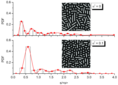
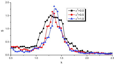
a)  b) c)

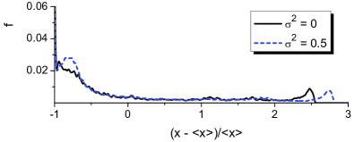
Figure 6: (a) Stationary probability density for vacancy clusters distribution over sizes $S$ for the deterministic ($\sigma^{2}=0$) and stochastic ($\sigma^{2}=0.5$) cases. (b) Spherically averaged structure function for the vacancy concentration at different noise intensities at $t=800$. Other parameters are: $T=773$K, $K=10^{-6}~{}dpa/sec$. (c) Distribution functions over vacancy clusters occupancy at deterministic and stochastic conditions

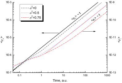
a)  b)

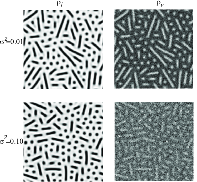
Figure 7: (a) Dynamics of the averaged sink densities $\langle\rho_{i}\rangle$, $\langle\rho_{v}\rangle$ for the different values of the external noise intensity under reactor conditions. (b) Typical snapshots of sinks distribution at different noise intensities at $t=700$.

Considering a behavior of sink densities $\langle\rho_{i}\rangle$, $\langle\rho_{v}\rangle$ one finds that during the system evolution the corresponding averages grow continuously with the irradiation dose increase (see Fig.7a). It means that interstitial and vacancy loops attracting vacancies grow in time due to positive feedback with vacancy field dynamics. The external noise decreases the corresponding averages. The most essential contribution of the noise can be seen on the sink density $\langle\rho_{i}\rangle$. It is interesting to note that quantities $\langle\rho_{i}\rangle$, $\langle\rho_{v}\rangle$ behave themselves in linear manner at large time intervals, i.e., $\langle\rho_{i}(t)\rangle,\langle\rho_{v}(t)\rangle\sim t$. Such dynamics of the sink density $\langle\rho_{v}\rangle$ is well observed even at early stages of the system evolution, whereas linear growth of $\langle\rho_{i}\rangle$ is realized at $t\gg 1$ only. The noise action suppresses dynamics of $\langle\rho_{i}\rangle$ at initial stages moving the universal part of its evolution toward large time scales. Such delaying dynamics leads to a weak arrangement of sink densities. At large time intervals one has well-organized vacancy clusters, whereas fields of sink densities have weak spatial modulation (see snapshots of $\rho_{i}(\mathbf{r})$ and $\rho_{v}(\mathbf{r})$ at $t=1000$ at different noise intensities in Fig.7b). In such a case the distributions of fields $\rho_{i}(\mathbf{r})$ and $\rho_{v}(\mathbf{r})$ are quite noisy.

IV.2 Patterning under accelerator conditions

Let us examine behavior of the system under accelerator conditions. Here we consider the typical case of $T=900K$ and $K=10^{-3}~{}dpa/sec$. In the corresponding simulations due to large damage rate $K$ the related time step is $\Delta t=15\times 10^{-5}$ in order to stabilize the numerical scheme.

Comparing dynamics of the averaged vacancy concentration under reactor and accelerator conditions one finds that in the second case the defects arrangement occurs essentially faster (cf.Fig.5 and Fig.8a). Moreover, number of defects increases by an order. The variance $\langle(\delta x)^{2}\rangle$ takes large values by two orders comparing to the previous case. It means that there is high difference in defect concentrations over the whole system. At high damage rate defects arrange into spherical clusters without extended structures (see Fig.8b). At such conditions the noise influence is opposite to the previous case: here due to combined effect of high-speed defect production and fluctuation influence the number of defects increases but fluctuations promote formation of vacancy clusters of a similar size. Considering spatial organization of fields $\rho_{i}$ and $\rho_{v}$ it is seen that even at large noise intensity there is well defined spatial structure of sink densities.

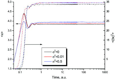
a)  b)

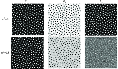
Figure 8: (a) Dynamics of the averaged concentration density and the corresponding variance for different values of the external noise intensity under accelerator. (b) Typical snapshots of vacancy concentration field and sinks distribution in deterministic and stochastic cases at $t=700$.

Comparing distributions of vacancy clusters by the size $s$ in deterministic and stochastic cases it follows that external fluctuations lead to vacancy migration between clusters. As a result $s$ attains the mean value $\langle s\rangle$ (see top panels in Fig.9). The noise action does not influence on vacancy clusters densities $n/N^{2}$ essentially, the number of clusters slightly grows with an increase in $\sigma^{2}$.

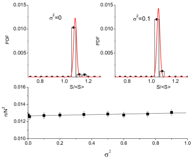
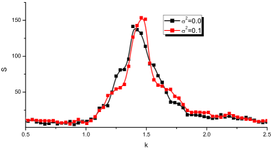
a) b) c)

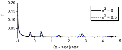
Figure 9: (a) Stationary distribution of vacancy clusters (at $\sigma^{2}=0$ and $\sigma^{2}=0.5$) and density of vacancy clusters versus noise intensity $\sigma^{2}$. (b) Structure function for vacancy concentration field at deterministic and stochastic conditions ($\sigma^{2}=0.1$). (c) Distribution functions over vacancy clusters occupancy at deterministic and stochastic conditions Other parameters are: $T=900K$ and $K=10^{-3}~{}dpa/sec$.

Considering behavior of the spherically averaged structure function of the vacancy concentration field shown in Fig.9b it follows that the external noise shifts slightly the peak position leading to formation of clusters distributed with small period. With the noise intensity growth the area under the curves $S(k)$ increases that well corresponds to elevated values of the order parameter $\langle(\delta x)^{2}\rangle$ in the stochastic case. Comparing data for the period of vacancy clusters $L_{0}$ related to the same data for irradiation under reactor conditions one gets $L_{0}\sim(4.5\div 4.2)\chi L_{d}$. The lower value of $L_{0}$ relates to large noise intensities. In other words vacancy clusters emerging at irradiation under accelerator conditions decrease down to $6.25\div 6.6\%$ under the same stochastic conditions. For the averaged linear size of vacancy clusters one has $\langle d_{0}\rangle\simeq 1.25\chi L_{d}\simeq 7.5~{}nm$. The distribution function $f(x)$ of vacancy clusters occupation is shown in Fig.9c for both deterministic and stochastic cases. In contrast to the previously studied case here the most of clusters are characterized by elevated vacancy concentration $x>\langle x\rangle$. It is principally important that the external fluctuations act in opposite manner comparing to the stochastic case discussed above. Indeed, here due to formation of mostly spherical clusters the stochastic contribution decreases vacancy concentration in clusters shifting main peaks of $f(x)$ toward small $x$. It is interesting to note that the maximal value of the distribution function in the point $x=0$ is larger by an order comparing to the same value under reactor conditions. It means that irradiation under accelerator conditions results to fast motion of vacancies to clusters leading to an emergence of a dense state of material without vacancies: the diffusion processes are suppressed here and all vacancies are collected in clusters.

Studying dynamics of sink densities (see protocol shown in Fig.10) one finds here that the linear growth law is observed, i.e., $\langle\rho_{v}(t)\rangle,\langle\rho_{i}(t)\rangle\propto t$. Comparing behavior of the sink densities at irradiation under reactor conditions with data shown in Fig.10 it follows that at large defect production rate $K$ the universal growth law is realized even at initial stages of the system evolution. There is no delayed dynamics caused by diffusion processes. The external fluctuations decrease values for sink densities as in previous case without delaying dynamics. At large $K$ one gets sink densities by three orders larger than under reactor conditions.

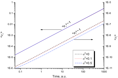
Figure 10: Dynamics of sink densities at different values for the noise intensity $\sigma^{2}$ at $T=900K$ and $K=10^{-3}~{}dpa/sec$.

V Conclusions

In this paper we have studied self-organization processes of vacancy clusters in stochastic system of point defects subjected to irradiation under reactor and accelerator conditions. As a prototype physical model the pure nickel with initial equilibrium vacancy concentration is used. We have considered a general case by taking into account dynamics of interstitial and vacancy loops. Within the framework of analytical and numerical analysis we have shown that free vacancies can arrange in defect clusters of nano-meter size. Obtained results are in good correspondence with experimental data (see Refs.JES ; Kiritani00 ; SYMK2004 ; Mazias ) and theoretical predictions Walgraef95 ; Walgraef ; mirz1 .

Using mean field approximation for the one-component system we have found critical values of both irradiation temperature and damage rate limiting self-organization of vacancies into clusters. From obtained numerical data we conclude that spatial arrangement of defects under both reactor and accelerator conditions differs by spatial modulation of vacancy concentration and sink densities fields. From the other hand values of the corresponding averaged quantities differ by three orders. The universal linear growth law for sink densities is observed at early stages of the system evolution due to high speed of point defects arrangement at high damage rates. It is principle important that in both studied cases the external fluctuations accelerate spatial organization of defects. However, under reactor conditions the external noise decreases the averaged point defects concentration, whereas at irradiation in accelerators such noise increases the corresponding value. In the stochastic case one has lower sink densities than in deterministic case. The noise delays dynamics of the sink densities essentially under irradiation in reactor conditions. We have found that period of vacancy clusters decreases with the noise intensity growth. Moreover, comparing the corresponding data it was shown that irradiation at elevated temperatures and high defect production rate decreases the period of vacancy clusters down to $6.5\%$. From obtained results for linear sizes of vacancy clusters it follows that the irradiation in accelerators leads to decrease of the linear size of vacancy clusters comparing to irradiation in reactors down to $20\%$. We have found that this characteristic does not depend on the intensity of external fluctuations. Such difference in linear sizes (period of structures and their diameter) at irradiation under reactor and accelerator conditions relates to large difference in defect production rate leading to different speeds of the corresponding diffusion processes. The same situation is clearly seen from dynamics of defect sinks. Studying distribution functions of vacancy clusters occupation we have found that one has fast organization of vacancy clusters with dense state of material without free vacancies under accelerator conditions due to suppressed diffusion processes comparing to the case of irradiation under reactor conditions. The external noise increases the vacancy concentration in clusters under reactor conditions, whereas it decreases an occupation of vacancy clusters at irradiation in accelerators.

References

- (1) A.Jostobns, K.Farrel, Rad.Effects, 15, 217 (1972)
- (2) J.O.Steigler, K.Farrel, Scr.Metall., 8, 651 (1974)
- (3) J.H.Evans, Nature, 229, 403 (1971)
- (4) J.E.Evans, D.J.Mazey, J.Nucl.Mat., 138, 176 (1986)
- (5) S.Saass, B.L.Eyre, Phil.Mag., 27, 1447 (1973)
- (6) P.B.Johnson, D.J.Mazey, J.H.Evans, Rad.Effects, 78, 147 (1983)
- (7) D.J.Mazey, J.E.Evans, J.Nucl.Mat., 138, 16 (1986)
- (8) R.Cuerno, A.-L.Barabasi, Phys.Rev.Lett., 74, 4746 (1995)
- (9) M.A.Makeev, A.-L.Barabasi, NIMB, 222, 316 (2004)
- (10) D.O. Kharchenko, V.O. Kharchenko, I.O. Lysenko, and S.V. Kokhan, Phys. Rev. E, 82, 061108 (2010)
- (11) V.O. Kharchenko, D.O. Kharchenko, Cond.Mat.Phys., 14, N2, 23602 (2011)
- (12) I.O.Lysenko, V.O.Kharchenko, S.V.Kokhan, A.V.Dvornichenko, Metallofiz.Noveishie Tekhnol., 35, N6, 763 (2013)
- (13) Vasyl O.Kharchenko, Dmitrii O.Kharchenko, Sergei V.Kokhan et al, Phys.Scr., 86, 055401 (2012)
- (14) V.O. Kharchenko, D.O. Kharchenko, Phys.Rev.E, 86, 041143 (2012)
- (15) Dmitrii O.Kharchenko, Vasyl O.Kharchenko, Irina O.Lysenko, Phys.Scr., 83, 045802 (2011)
- (16) Dmitrii O.Kharchenko, Vasyl O.Kharchenko, Tetyana Zhylenko, Alina V.Dvornichenko, Eur.Phys.J.B, 86, 175 (2013)
- (17) G.Martin, Phys.Rev.B., 30, 1424 (1984)
- (18) P.A.Selischev, V.I.Sugakov, Rad.Effects, 133, 237 (1995)
- (19) L.A.Maksimov, A.I.Ryazanov, Sov.Phys.JETP, 52(6), 1170 (1980)
- (20) N.M.Ghoniem, D.Walgaef, Modeling Simul.Mat.Sci.Eng., 1(5), 569 (1993)
- (21) C.Abromeit, G.Martin, J.Nuc.Mat., 271&272, 251 (1999)
- (22) Vasyl O.Kharchenko, Dmitrii O.Kharchenko, Eur.Phys.Jour.B 85, 383 (2012).
- (23) V.O.Kharchenko, D.O.Kharchenko, Condens. Matter Phys. 16, N3, 33001 (2013).
- (24) T.S.Byun, K.Farrell, J.Nucl.Mater., 326, 86 (2004)
- (25) V.I.Dubinko, S.A.Kotrechko, V.F.Klepikov, Radiat.Eff.Def.Solids, 164, 10, 647 (2009)
- (26) R.Chaouadi, R.Geŕard, J.Nucl.Mater., 345, 65 (2005)
- (27) Yu.N.Osetsky, D.J.Bacon, A.Serra, B.N.Singh, and S.I.Golubov, J.Nucl.Mater., 276, 65 (2000)
- (28) V.Gavini, K.Batthacharya, and M.Ortiz, Phys.Rev.B, 76, 180101 (2007)
- (29) N.M.Ghoniem, D.Walgraef, Modelling Simui. Mater. Sci. Eng. 1, 569 (1993)
- (30) D.Walgraef, J.Lauzeral, N.M.Ghoniem, Phys,Rev.B, 53, 14782 (1996)
- (31) Daniel Walgraef Spatio-Temporal Pattren Formation (Springer-Verlag, New York, Berlin, Heidelberg, 1996).
- (32) D.Walgraef, N.M.Ghoniem, Phys,Rev.B, 67, 064103 (2003)
- (33) F.Kh.Mirzoev, V.Ya.Panchenko, L.A.Shelepin, Physics Uspekhi, 39, 1 (1996)
- (34) W.Jager, P.Ehrhart, W.Shchilling, in Nonlinear Phenomena in Material Science, ed.by G.Marten and I.P.Kubin (Transtech addr Aedermannsorrf, Switzerland, 1988), p.279
- (35) M.Kiritani. T.Yoshiie, S.Kojima, Y.Satoh, Radiat.Eff.Def.Solids. 113, 75 (1990)
- (36) M.Kiritani, H.Takata, J.Nucl.Mater., 69, 27 (1978)
- (37) Michio Kiritanim, J.Nucl.Mater.,276, 41 (2000)
- (38) Y.Satoh, T.Yoshiie, H.Mori, M.Kiritani, Phys.Rev.B, 69, 941081 (2004)
- (39) P.J.Maziasz, J.Nucl.Mater.,169, 95 (1989)
- (40) M.Kiritani, J.Nucl.Mater., 216, 220 (1994)
- (41) R.Enrique, P.Bellon, Phys.Rev.Lett., 84, 2885 (2000).
- (42) R.A.Enrique, P.Bellon, Phys.Rev.E, 63, 134111 (2001).
- (43) Jia Ye, P.Bellon, Phys.Rev.B,70, 094104 (2004).
- (44) Michio Kiritani, Ultramicroscopy, 39, 135 (1991)
- (45) Tomas Diaz de la Rubia, Hussein M.Zbib, Tariq A.Kharaishi, et al., Nature, 406, 871 (2000)
- (46) B.D.Wirdh, M.J.Caturla, T.Diaz de la Rubia, et al., NIMB, 180, 23 (2001)
- (47) Chu-Chun Fu, Jacques Dalla Torre, Francois Willaime, et al., Nature Materials, 4, 68 (2005)
- (48) M.Kiritani, Mat.Chem.Phys., 50, 133 (1997)
- (49) V.I.Dubinko, A.V.Tur, A.A.Turkin, V.V.Yanovsky, Rad.Eff. 112, 233 (1990)
- (50) D.O.Kharchenko, I.O.Lysenko, S.V.Kokhan, Eur.Phys.J.B. 76, 37 (2010).
- (51) D.Kharchenko, I.Lysenko, V.Kharchenko, Physica A 389, 3356 (2010).
- (52) D.O. Kharchenko, V.O. Kharchenko, I.O. Lysenko, Cent.Eur.J.Phys. 9, N.3, 698 (2011).
- (53) D.O.Kharchenko, V.O.Kharchenko, S.V.Kohan, I.O.Lysenko, Ukr.Jour.Phys., 57, N.10, 1069 (2012)
- (54) D.O.Kharchenko, V.O.Kharchenko, A.I.Bashtova, Ukr.Jour.Phys., 58, N.10, 993 (2013)
- (55) F.Kh.Mirzoev, V.Ya.Panchenko, L.A.Shelepin,, Techn.Phys.Lett., 22, 13, 28, (1996)
- (56) D.Batogkh, M.Hildebrant, F.Krischer, A.Mikhailov, Phys.Rep. 288, 435 (1997).
- (57) D.O.Kharchenko, S.V.Kokhan, A.V.Dvornichenko, Physica D, 238, 2251 (2009)
- (58) D.O.Kharchenko, S.V.Kokhan, A.V.Dvornichenko, Metallofiz.Noveishie Tekhnol., 31(1), 23 (2009)
- (59) J.Garcia-Ojalvo, J.M.Sancho, Noise in Spatially Extended Systems, Springer, New York, 1999.
- (60) H.Risken The Fokker-Planck equation (Springer-Verlag, Berlin, 1984).