How does a magnetic trap work?

Abstract

Magnetic trapping is a cornerstone for modern ultracold physics and its applications (e.g., quantum information processing, quantum metrology, quantum optics, or high-resolution spectroscopies). Here a comprehensive analysis and discussion of the basic physics behind the most commonly used magnetic traps in Bose-Einstein condensation is presented. This analysis includes the quadrupole trap, the time-averaged orbiting potential trap, and the Ioffe-Pritchard trap. It is shown how the trapping conditions and efficiency of these devices can be determined from simple derivations based on classical electromagnetism, even though they operate on quantum objects.

I Introduction

In 1995 the first Bose-Einstein condensates (BECs) were synthesized experimentally.Anderson et al. (1995); Davis et al. (1995); Bradley et al. (1995) Ever since, ultracold physics as well as its applications (e.g., quantum information processing, quantum metrology, quantum computation, quantum optics, high-resolution spectroscopies, etc.) have undergone a remarkable development.Carr et al. (2009) In the ultracold regime, the particles (atoms or molecules) that constitute the condensate have to behave as a whole, i.e., they must constitute a coherent cloud, as if they all just formed a single particle. In order to observe this behavior, the thermal de Broglie wavelength, $\lambda_{\rm dB}$, of the species considered has to be at least of the order of magnitude of the cloud size. This means that $\lambda_{\rm dB}\gtrsim n^{-1/3}$, with $n$ being the particle density. Under these circumstances, the condensate dynamics will be completely dominated by quantum effects.Griffin, Snoke, and Stringari (1995); Dalfovo et al. (1999); Legget (2001); Pethick and Smith (2002)

One of the methods utilized to reach the ultracold regime is the process known as evaporative cooling.Hess (1986); Ketterle and van Druten (1996) According to this method, first an ensemble of particles (cloud) that follows a Maxwell-Boltzmann velocity distribution is confined within a magnetic trap (it could also be a dipolar trap). Then, the most energetic particles will escape from the trap due to their higher energy, while the less energetic ones will remain inside it. The net effect is thus an effective cooling, similar to the process leading coffee in a cup to cool down, for example. In order to reach thermalization by inter-particle elastic collisions at very low temperatures, the walls of the trap are also lowered. This produces an increment of the particle loss rate, which eventually leads the remaining particles to condensate.

Magnetic trapping has its origins in plasma physics, where the confinement of charged particlesMiley et al. (2000); Goldstone and Rutherford (2000) is one of the main steps in the control of fusion reactions that take place inside plasmas. The first technique employed to trap and confine charged particles within this field was the so-called magnetic bottle configuration, which results from the combination of two magnetic mirrors. In this configuration the trapped particles bounce back and forth periodically between the two mirrors (turning points), where the intensity of the magnetic field is relatively high, thus preventing the particles from escaping.Allen (1962)

The magnetic bottle configuration described above cannot be directly applied to BECs, because they are neutral particles. Nevertheless, magnetic trapping in this case still relies on the same basic idea, although it involves a different trapping mechanism, namely the combination of the Zeeman effect with Earnshaw’s theorem.Earnshaw (1842); Wing (1984) On the one hand, the Zeeman effect originates the splitting of the particle energy levels in the presence of a magnetic field due to the interaction between this field and the particle magnetic dipole moment. On the other hand, Earnshaw’s theorem determines the properties of a particular magnetic field configuration, thus playing a key role in the understanding of neutral particle trapping.

With this in mind, it is then clear that a proper knowledge of the functioning of neutral-particle magnetic trapping is fundamental to understanding modern ultracold physics.Wieman (1996); Carr et al. (2009) The motivation and purpose of this work is to explain the essential elements of magnetic trapping in simple terms. In particular, we have focused on basic physical properties of the three most relevant configurations used in this research field, namely the quadrupole trap, the time-averaged orbiting potential (TOP) trap, and the Ioffe-Pritchard trap. As it is shown, the trapping conditions and efficiency of these devices can be determined from simple derivations obtained from classical electromagnetism. From a pedagogical viewpoint, we consider that this has a potential interest in elementary courses on classical electromagnetism, for it relates in an easy fashion this field of physics with quantum mechanics through the quantum nature of BECs (actually, without making a explicit use of quantum mechanics).

The work is organized as follows. To be self-contained, in Sec. II we present a brief account on the role of the Zeeman effect and Earnshaw’s theorem in magnetic trapping. The description of the traps mentioned above and their properties, such as performance and efficiency, are introduced in Sec. III, while a comparative analysis is given in Sec. IV. Usually we find in the literaturePethick and Smith (2002) that the magnetic scalar field (or potential) for a trap is introduced ad hoc, in terms of some plausibility arguments. In this regard, our work complements a previous one by Gov et al.,gov also published in this journal, where the authors present a classical and quantum-mechanical analysis of neutral-particle magnetic trapping. The derivations presented in Sec. III are, however, very simple and readily lead to the trapping condition. Finally, a series of remarks drawn from this work are summarized in Sec. V.

II Zeeman effect and Earnshaw’s theorem

According to classical electromagnetism,Jackson (1999); Smythe (1989); Jefimenko (1989); Pafosky and Philips (2005) the energy of a magnetic dipole moment, ${\boldsymbol{\mu}}$, acted by an external magnetic field, ${\bf B}$, is given by

$$E=-\boldsymbol{\mu}\cdot{\bf B}.$$ (1)

Quantum-mechanically this interaction produces a splitting of the particle (quantum) energy levels, namely the so-called Zeeman effect.Brown and Carrington (2003) In atoms or molecules, the total magnetic dipole moment is specified by the orbital angular momentum and spin of the electrons from the valence shell. This quantity reads asBrown and Carrington (2003)

$$\boldsymbol{\mu}=-g_{s}\mu_{B}{\bf S}-g_{l}\mu_{B}{\bf L},$$ (2)

where $g_{s}\approx 2.002319$ is the electron spin $g$-factor,Odom et al. (2006) ${\bf S}$ is the magnitude of the electron spin angular momentum, $g_{l}=1$ is the electron orbital $g$-factor, ${\bf L}$ is the magnitude of the electron orbital angular momentum, and $\mu_{B}=e\hbar/2m_{e}=0.67$ K/T is the Bohr magneton.

An illustration of the Zeeman splitting in the case of a realistic system, namely the ¹⁶O${}_{2}(^{3}\Sigma_{g}^{-})$ molecule,Brown and Carrington (2003) is displayed in Fig. 1. A detailed account of the calculations performed to obtain the results displayed in this figure goes beyond the scope of the present work due to the different technical (numerical) computational aspects involved. Nonetheless, for reproducibility purposes, the interested reader can find the relevant realistic parameters used in these calculations in Mizushima’s The Theory of Rotating Diatomic Molecules.Mizushima (1975) These parameters are the rotational constant ($B_{e}=1.438$ cm^-1), the spin-rotation interaction constant ($\gamma_{\rm SR}=-0.0089$ cm^-1), and the spin-spin coupling constant ($\gamma_{\rm SS}=1.985$ cm^-1).

In this example, the splitting of the energy levels comes only from the interaction between the molecular electronic spin and the external magnetic field, since the valence-shell electrons for molecules in a ${}^{3}\Sigma$ electronic state have a zero orbital angular momentum.Brown and Carrington (2003) As can be seen, two different responses of the molecular internal states are found. There are levels that increase their energy with the intensity of the magnetic field (blue dashed lines), which are called low-field seekers and are stable at low intensities (the concept of stability here refers to the system energetic configuration, which should be distinguished from the concept of dynamical stability; see below, in Sec. IV). On the contrary, there are high-field seeker states (red solid lines), which display an energy decrease as the field intensity increases, thus being stable in regions of higher or more intense magnetic fields.

Taking these facts into account, a priori one would be willing to design magnetic field configurations either with a local minimum to trap low-field seeker states, or with a local maximum to trap high-field seeker states. The second option, though, is forbidden in virtue of the so-called Earnshaw’s theoremEarnshaw (1842); Wing (1984) (for a historical account on Samuel Earnshaw, the discoverer of this theorem, we refer the interested reader to the work by William Scott in this same journal.Scott (1959)) According to this theorem, in the absence of currents the modulus of the magnetic field, $B\equiv|{\bf B}|$, has no local maxima —the same result, as formerly shown by Earnshaw,Earnshaw (1842) applies to the electric field whenever the region under study is free of charge.Jefimenko (1989) Therefore, in practice the design of magnetic traps reduces to finding configurations with a local minimum, which are suitable to trap low-field seeker states.

III Types of magnetic traps

From the discussion presented in Sec. II, it follows that the basic ingredient involved in the design of an optimal trap consists in finding an arrangement of coils and wires that produces a magnetic field with the desired minimum. The purpose of this trap is to confine an atomic or molecular cloud of a size much smaller than the typical dimensions of the experimental magnetic arrangements. Notice that typical cloud densities are $n\sim 10^{12}$–$10^{14}$ cm^-3, so that cloud sizes are in the range $n^{-1/3}\sim 0.1$–$1$ $\mu$m, while the radii of coils and the distances between coils and wires are of the order of centimeters! Accordingly, one only needs to be concerned with the characteristics of the magnetic field in a vicinity of its minimum, which allows for simplifying series expansions around it, as seen below.

Typical magnetic traps display azimuthal symmetry, since the coils playing the role of magnetic mirrors are of the same dimensions, parallel one another, and centered around the azimuthal axis ($z$), as seen in Fig. 2. Accordingly, the minimum not only will appear along the azimuthal axis, but at the origin of the coordinate system. Of course, gravity will affect the position of this minimum, by moving it downwards. However, in the analysis presented in this work we will not include gravity for simplicity and also because it gives rise to other types of effects, such as chaotic dynamics.Metcalf and vad der Straten (2007) In order to obtain and analyze the magnetic field around the local minimum, we can derive the exact expression for the off-axis magnetic field or from the corresponding magnetic scalar field, $\Phi$. Then, a Taylor series expansion around the minimum is performed. These two fields are related through the expressionPafosky and Philips (2005)

$${\bf B}=-\nabla\Phi,$$ (3)

since no currents are present between the coils.

The magnetic scalar potential $\Phi$ satisfies the Laplace equation $\nabla^{2}\Phi=0$ (equivalent to $\nabla\cdot{\bf B}=0$). Hence it admits a general solution in spherical coordinates,Jackson (1999); Smythe (1989); Pafosky and Philips (2005); Jefimenko (1989)

$$\Phi=\sum_{\ell,m}\left[C_{\ell,m}r^{\ell}+D_{\ell,m}r^{-(\ell+1)}\right]Y_{\ell}^{m}(\theta,\phi),$$ (4)

where $Y_{\ell}^{m}$ is the spherical harmonic function of degree $\ell$ and order $m$; the $C_{\ell,m}$ and $D_{\ell,m}$ coefficients describe, respectively, the near and far field from the current distribution, being dependent on its geometry and intensity. Because trapping is assumed to occur in the near field and the system displays azimuthal symmetry (no dependence on the azimuthal angle $\phi$), Eq. (4) can be recast as

$$\Phi=\sum_{\ell}C_{\ell}r^{\ell}P_{\ell}(\cos\theta),$$ (5)

with $\ell$ labeling the multipole moment.

Now we already have the essential tools to conduct our analysis of the different types of magnetic traps.

III.1 Quadrupole trap

The quadrupole trap is the simplest magnetic trap that can be devised. It is obtained by positioning the two coils in anti-Helmholtz configuration, i.e., with their currents flowing in opposite directions [see Fig. 2(a)]. The total field can be obtained as the sum of the fields generated by each coil. So, in order to determine the trapping field, let us first consider a current $I_{c}$ flowing along a single coil of radius $a$. The general expression for the magnetic field generated by such a coil is analytical, expressible in terms of the complete elliptic integrals.Jackson (1999) As mentioned above, the minimum will appear along the azimuthal axis, so we will only be concerned with the behavior of the field along this axis. In such a case, the magnetic scalar potential reads as

$$\Phi_{c}(z)=-\frac{\mu_{0}I_{c}}{2}\frac{z}{\sqrt{z^{2}+a^{2}}},$$ (6)

where $\mu_{0}$ is the vacuum magnetic permittivity. If now we take into account the contribution coming from each coil, placed at $z=b$ and $z=-b$, the total magnetic scalar potential is given by

$$\Phi(z)=-\frac{\mu_{0}I_{c}}{2}\left[\frac{z-b}{\sqrt{(z-b)^{2}+a^{2}}}-\frac{z+b}{\sqrt{(z+b)^{2}+a^{2}}}\right].$$ (7)

As said above, the typical sizes for trapped clouds are much smaller than the length scales associated with the magnetic arrangement. Thus, under the assumption that $z\ll a,b$, Eq. (7) can be approximated by

$$\Phi(z)=\frac{\mu_{0}I_{c}}{2}\left[\frac{2b}{\left(a^{2}+b^{2}\right)^{1/2}}-\frac{3a^{2}bz^{2}}{\left(a^{2}+b^{2}\right)^{5/2}}\right],$$ (8)

where we notice that only even powers of $z$ play a role.

After comparing Eq. (5) with (8), we can reasonably argue that the sum in (5) should also run only over even values of $l$. Indeed, we can also assume that the off-axis magnetic field is the straightforward generalization of the on-axis one, given by (8). Under these hypotheses, we obtain $C_{0}=\mu_{0}I_{c}b/\sqrt{a^{2}+b^{2}}$, $C_{2}=-3\mu_{0}I_{c}a^{2}b/2(a^{2}+b^{2})^{5/2}$, and $C_{\ell}=0$ for $\ell>2$, at least at the order of the approximations here considered. Rewriting the resulting expression in cylindrical coordinates ($r=\sqrt{\rho^{2}+z^{2}}$ and $\cos\theta=z/r$), we find that

$$\Phi(\rho,z)=C_{0}+\frac{C_{2}}{2}\left(2z^{2}-\rho^{2}\right).$$ (9)

From Eq. (3), the magnetic field is readily found, which in Cartesian coordinates reads as

$${\bf B}=-C_{2}\left(x{\bf u}_{x}+y{\bf u}_{y}-2z{\bf u}_{z}\right).$$ (10)

As seen, the gradient of this field with vanishing divergence is ruled by $C_{2}$, i.e., the size and distance between the coils. As it can be seen from the modulus of the magnetic field,

$$B=\|{\bf B}\|=C_{2}\sqrt{x^{2}+y^{2}+4z^{2}},$$ (11)

this trap can never be perfectly harmonic.

According to Eq. (11), the magnetic field of a quadrupole trap has a zero minimum at the origin. Hence, if the trapped particles reach the minimum, the energy spacing between Zeeman levels becomes rather reduced (see Fig. 1). This increases the probability of non-adiabatic transitions among these energy levels, leading to a loss of particles in the trap. This scape mechanism is known as spin-flip Majorana transition.Majorana (1932); brink

III.2 TOP trap

The TOP trap is a modification of the quadrupole trap, which skips the inconvenience of the zero-field minimum. More specifically, this modification consists of adding a time-dependent rotating bias field in the $XY$-plane, so that

$${\bf B}=(C_{2}x+B_{b}\cos\omega t){\bf u}_{x}+(C_{2}y+B_{b}\sin\omega t){\bf u}_{y}-2C_{2}z{\bf u}_{z}.$$ (12)

This makes the minimum to revolve around the center of the trap in a circle of radius $R=B_{b}/C_{2}$. This is better seen by computing the modulus of this magnetic field,

$$B=\sqrt{(C_{2}x+B_{b}\cos\omega t)^{2}+(C_{2}y+B_{b}\sin\omega t)^{2}+4C_{2}^{2}z^{2}}.$$ (13)

The bias frequency, $\omega$, provides us with information about the working regime. In order to select an optimal trapping regime, $\omega$ has to satisfy two conditions:

1. It should be larger than the oscillation frequency of the trapped particles ($\sim 100$ Hz), so that they will feel an effective time-averaged magnetic field.

2. It should be smaller than the frequency associated with the transition between two consecutive internal quantum states ($\sim 10^{6}$ Hz) to prevent particle losses by spin-flip Majorana transitions.

In the particular case that we are interested in, we have $r=\sqrt{x^{2}+y^{2}+z^{2}}\ll R$, and Eq. (12) can be approximated by

$$B=B_{b}+\frac{C_{2}^{2}}{2B_{b}^{2}}\ \!(x^{2}+y^{2}+4z^{2})+\frac{C_{2}}{B_{b}}\ \!(x\cos\omega t+y\sin\omega t)-\frac{C_{2}^{2}}{2B_{b}^{2}}\ \!(x\cos\omega t+y\sin\omega t)^{2}.$$ (14)

From this expression, we can now obtain the effective time-averaged magnetic field felt by the trapped particles,

$$\bar{B}=\frac{\omega}{2\pi}\int_{0}^{2\pi/\omega}B(t)dt=B_{b}+\frac{C_{2}^{2}}{4B_{b}}\ \!(x^{2}+y^{2}+8z^{2}).$$ (15)

As it can be noticed, the effect of the bias is to generate an (effective) anisotropic harmonic potential, with an energy origin shifted upwards in energy ($B_{b}$) and frequencies $\omega_{x}=\omega_{y}=\sqrt{-\mu C_{2}^{2}/2mB_{b}}$ and $\omega_{z}=\sqrt{-4\mu C_{2}^{2}/mB_{b}}$, where $m$ is the mass of the trapped species. These frequencies arise after substitution of Eq. (15) in the expression for the magnetic interaction energy (1). We thus obtain an effective interaction potential, such that $\mu=-dE/dB<0$ for low-field seeker states according to Fig. 1.

III.3 Ioffe-Pritchard trap

In the traps that we have just analyzed, we were mainly concerned about trapping conditions along the azimuthal direction. We also ended up getting some trapping along the radial direction, although this was not the main goal. In order to determine specific trapping conditions along this direction, it is necessary to introduce an additional constraining field. In practice, this is achieved by incorporating a series of wires around the two coils, as it happens in Ioffe-Pritchard traps [see Fig. 2(b)]. In this trap, four wires are suited at the corners of a square, with the currents flowing along adjacent wires being of opposite sign (see Fig. 3).

Let us start again by first considering the case of a current $I_{w}$ flowing along a single, straight wire. The magnetic field generated by this wire is given by

$${\bf B}=-\frac{\mu_{0}I_{w}}{2\pi}\left(\frac{y{\bf u}_{x}-x{\bf u}_{y}}{x^{2}+y^{2}}\right).$$ (16)

This expression can be easily obtained from Ampere’s law (in this case, determining the magnetic field from this law is simpler than doing it through the magnetic scalar potential) and taking into account the transformation relations of unitary vectors from cylindrical to Cartesian coordinates

$$\begin{array}[]{rcl}{\bf u}_{\rho}&=&\cos\phi{\bf u}_{x}+\sin\phi{\bf u}_{y}\\ {\bf u}_{\phi}&=&-\sin\phi{\bf u}_{x}+\cos\phi{\bf u}_{y}\end{array}.$$ (17)

(Actually, from symmetry considerations, we can see that only ${\bf u}_{\phi}$ is necessary.)

The total magnetic field generated by the four wires can be now readily obtained from (16) if we evaluate this expression at the points $(x+d,y+d)$, $(x-d,y+d)$, $(x-d,y-d)$, and $(x+d,y-d)$, instead of $(x,y)$, and we add the four resulting fields. Then, as before, assuming $d\gg x,y$, we obtain

$${\bf B}=\frac{\mu_{0}I_{w}}{\pi d^{2}}\left(x{\bf u}_{x}-y{\bf u}_{y}\right).$$ (18)

A cross-section of this field is displayed in Fig. 3, where the length of the (blue) arrows is proportional to the field intensity. As it can be seen, we observe that these arrows point towards the origin (upwards or downwards) along the axis $x=0$, and outwards the origin (leftwards or rightwards) along the axis $y=0$. From a dynamical point of view,jordan the first axis is called stable and the second, unstable; the origin is called a saddle or hyperbolic point. To better understand the dynamical implications of this fact, consider a system directly acted by the magnetic field (18). If this system is released at some point $y_{0}$ and $x_{0}=\epsilon$, with $\epsilon\to 0$, it will fall towards $y=0$, separating from the $x=0$ axis slowly initially and then very rapidly as it approaches the unstable axis, $y=0$. These points are, for example, at the origin of chaotic behaviors or high sensitivity to initial conditions (e.g., exponential divergence between two trajectories that are launched from very close initial conditions).

The presence of the saddle point is a direct consequence of the quadrupolar nature of the arrangement in the radial direction. However, the same point becomes a stable minimum for the modulus of the magnetic field,

$$B=\frac{\mu_{0}I_{w}}{\pi d^{2}}\ \!\sqrt{x^{2}+y^{2}}.$$ (19)

In this case, again from a dynamical point of view, this means that a particle acted by (19) instead of ${\bf B}$ will always fall down to the origin, like an oscillator. This minimum can be seen in Fig. 4, where the magnetic field (19) is plotted along the $x$-axis [i.e., the unstable direction for (18)].

In the field of plasma confinement, this particular type of magnetic configuration, formed by the four bars, is known as Ioffe bars.Gott-62 In analogy to quadrupole traps, spin-flip Majorana transitions can also occur here due to the presence of a vanishing field minimum. To overcome this inconvenience, a homogeneous magnetic field along the azimuthal direction, $B_{h}{\bf u}_{z}$ is introduced, so that

$${\bf B}=\frac{\mu_{0}I_{w}}{\pi d^{2}}\left(x{\bf u}_{x}-y{\bf u}_{y}+z_{0}{\bf u}_{z}\right),$$ (20)

with $B_{h}=\mu_{0}I_{w}z_{0}/\pi d^{2}$. The modulus of this field is

$$B=\frac{\mu_{0}I_{w}}{\pi d^{2}}\ \!\sqrt{x^{2}+y^{2}+z_{0}^{2}},$$ (21)

which has a non-vanishing minimum due to the shift induced by the above homogeneous field (see Fig. 4), this avoiding the losses associated with spin-flip Majorana transitions. Obviously, this configuration changes the behavior of the magnetic field close to the minimum, from a linear dependence to a quadratic.

The homogeneous magnetic field as well as the confinement along the azimuthal direction can be generated if the two coils are arranged in Helmholtz configuration, i.e., making the intensities in each coil to flow in the same direction [see Fig. 2(b)]. In this case, the on-axis magnetic scalar potential reads as

$$\Phi(z)=-\frac{\mu_{0}I_{c}}{2}\left[\frac{z-b}{\sqrt{(z-b)^{2}+a^{2}}}+\frac{z+b}{\sqrt{(z+b)^{2}+a^{2}}}\right].$$ (22)

Then, assuming again $z\ll a,b$ and expanding for small $z$, we find

$$\Phi(z)=-\frac{\mu_{0}I_{c}}{2}\left[\frac{2a^{2}z}{\left(a^{2}+b^{2}\right)^{3/2}}-\frac{(a^{4}-4a^{2}b^{2})z^{3}}{\left(a^{2}+b^{2}\right)^{7/2}}\right],$$ (23)

which depends on odd of powers of $z$ due to the Helmholtz configuration of the coils. When comparing with Eq. (5), we find that now the sum will run over odd values of $\ell$. More specifically, we will have $C_{1}=-\mu_{0}I_{c}a^{2}/(a^{2}+b^{2})^{3/2}$, $C_{3}=\mu_{0}I_{c}a^{2}(a^{2}-4b^{2})/2(a^{2}+b^{2})^{7/2}$, and $C_{\ell}=0$ for $\ell>3$ (at the order of approximation considered). By using cylindrical coordinates, Eq. (23) can be recast as

$$\Phi(\rho,z)=C_{1}z+\frac{C_{3}}{2}\left(2z^{3}-3z\rho^{2}\right).$$ (24)

The corresponding magnetic field in Cartesian coordinates reads as

$${\bf B}=3C_{3}z\left(x{\bf u}_{x}+y{\bf u}_{y}\right)-\left[C_{1}-\frac{3}{2}\ \!C_{3}\left(x^{2}+y^{2}-2z^{2}\right)\right]{\bf u}_{z}.$$ (25)

In Eq. (25) we notice confinement along the azimuthal direction. This becomes more apparent if we consider the field along the azimuthal axis, for $x=0$ and $y=0$,

$$B_{z}=-C_{1}-3C_{3}z^{2}$$ (26)

(in this case, $B_{x}=B_{y}=0$). The first term is a homogeneous field, while the second is a quadratic trapping term related to the curvature of the magnetic field. Contrary to $C_{2}$ in the quadrupole trap, here $C_{3}$ has a sign that depends on the arrangement geometry, i.e., the radius of the coils, $a$, and their distance, $2b$. Thus, by selecting the coil parameters $a$ and $b$ in a convenient manner, one can generate more tightly trapping potentials, and also change their curvature (or even suppress it). In this sense, one could benefit from the relation $C_{3}\propto a-2b$: by choosing $a=2b$, we get the homogeneous field along the azimuthal axis needed to avoid spin-flip Majorana transitions in the radial direction, with $B_{h}=-C_{1}=8\mu_{0}I_{c}/5\sqrt{5}a$.

Now, given a particular arrangement of currents, a maximum magnetic field $B_{\rm max}$ is obtained. According to Eq. (1), this value determines the largest amount of energy accessible to the particles inside the trap, $E_{\rm max}=\mu(B_{\rm max}-B_{\rm min})$. Any particle with kinetic energy larger than $E_{\rm max}$ will escape from the trap. In this sense, $E_{\rm max}$ is defined as the trap depth. It is one of the parameters that has to be taken into account when designing magnetic traps, since it will give us an estimate of the number of trapped particles from among an ensemble characterized by a certain velocity distribution.Hess (1986); Ketterle and van Druten (1996) In Fig. 4, for example, this maximum amount of energy (horizontal lines) is expressed in terms of the corresponding field intensity. In particular, we have considered $B_{\rm max}-B_{\rm min}=10$ mT.

IV Discussion

Once we have seen the essential elements involved in the design of the three kind of traps used to produce and confine BECs, it is interesting to establish a comparative analysis in terms of their confinement efficiency. In this regard, we would like to specify that, within this context, by efficiency we mean the capability of a particular magnetic configuration to confine the particle cloud within a certain space region. This analysis can be carried out by investigating the magnetic field around the trap minimum.

As mentioned above, spin-flip Majorana transitions constitute a loss mechanism that has to be taken into account in order to set some control on the efficiency of a magnetic trap. The rate of non-adiabatic transitions between trapped and non trapped states increases when the magnetic configuration has a zero-field minimum, as happens in the quadrupole trap. Therefore, for low field intensities what one expects is that particle losses per time unit will be higher in quadrupole traps than in TOP or Ioffe-Pritchard ones.

Let us consider, though, the behavior of the field close to the (trap) minimum and analyze the energy of the particles inside the trap. Following Eq. (1), a suitable estimate of this energy is given byPetrich et al. (1995)

$$E\sim\mu B_{c}\left(\frac{n^{-1/3}}{a}\right)^{\ell-1},$$ (27)

where $\mu$ is the modulus of the atomic magnetic moment and $B_{c}$ is the magnetic field generated by the coils. As we saw in Sec. II, the maximum multipole moment for quadrupole traps is $\ell=2$, while for TOP and Ioffe-Pritchard traps is $\ell=3$. Accordingly, the interaction potential for the former (with vanishing minimum) is a factor $n^{-1/3}/a$ larger than for the latter (with non-vanishing minima). Typically, this factor ranges between 10 and 1,000, making the quadrupole trap to be more efficient than the TOP and Ioffe-Pritchard ones (in the sense indicated above).

We can also estimate the cloud density inside the magnetic trap, which can be expressed as a Maxwell-Botzmann distribution,

$$n({\bf r})=n_{0}e^{-U({\bf r})/k_{B}T},$$ (28)

where $n_{0}$ is the density at the center of the trap and $U({\bf r})$ is the trapping potential. The latter is obtained from the magnetic energy difference between a given value of the field and its minimum, i.e., from Eq. (1), $U({\bf r})=\Delta E=\mu[B({\bf r})-B_{\rm min}]$, with $\mu$ denoting the modulus of the magnetic dipole moment. The total number of trapped particles is thus given by

$$N=n_{0}\int e^{-U({\bf r})/k_{B}T}d{\bf r},$$ (29)

where the integral can be defined as the effective volume occupied by the particle cloud, $V_{\rm eff}\equiv\int e^{-U({\bf r})/k_{B}T}d{\bf r}$. In Fig. 5(a) we show the profile of the magnetic field along the $x$-direction (with $y=z=0$) for the three traps analyzed in the previous section (the parameters involved in the calculations are given in the figure caption); similarly, in Fig. 5(b) the same is done along the $z$-direction (with $x=y=0$). As we are going to see, independently of the minimum value, in this case the particle density is governed by the trap topology (curvature). Thus, for the quadrupole trap, from (11) the trapping potential reads as

$$U({\bf r})=\mu C_{2}\sqrt{x^{2}+y^{2}+4z^{2}}$$ (30)

and therefore $V_{\rm eff}\sim T^{3}$. However, if the behavior of the magnetic field is smoother around the trap minimum, as in TOP and Ioffe-Pritchard traps, the dependence on temperature will change. Taking as an example the TOP trap, with trapping potential

$$U({\bf r})=\frac{\mu C_{2}^{2}}{4B_{b}}\ \!(x^{2}+y^{2}+8z^{2}),$$ (31)

we find $V_{\rm eff}\sim T^{3/2}$.

From a practical point of view, we know that in order to reach the BEC state, the phase-space density, which goes as $n\lambda_{\rm dB}^{3}$, has to be increased by decreasing the particle temperature. Now, given a constant number of trapped particles, since the particle density $n_{0}$ is inversely proportional to $V_{\rm eff}$, from the above two behaviors we find that effectively it will increase as $T$ decreases. The variation of the density as a function of the temperature is displayed in Fig. 5(c) for the three types of magnetic traps considered in this work. For the chosen parameters (see figure caption for details), we notice that, at high temperatures, the particle density in a Ioffe-Pritchard trap is higher than in the other two ones, while as temperature decreases the opposite behavior is observed. A crossover for these trends is observed at $T\approx 3$ mK (other crossovers can also be seen at other temperatures).

Such a behavior with temperature is related to the shape of the magnetic field around the minimum, which has an important influence on the confinement or compression of the swarm of trapped particles per volume unit. More specifically, this compression is connected to the particle kinetic energy through the temperature of the sample. That is, at higher temperatures particles are able to visit regions with higher values of the potential energy, while at lower temperatures only regions closer to the minimum can be explored. This behaviors can be easily inferred by inspecting Fig. 5(a) in combination with Fig. 5(b). Thus, for low temperatures, in spite of the high confinement displayed by the Ioffe-Pritchard trap along the $x$-direction [see Fig. 5(a)], along the $z$-direction (for the $y$-direction it would be the same as for the $x$ one) the confinement is very poor [see Fig. 5(b)]. On the contrary, for the quadrupole trap the confinement is optimal along either direction, thence the confining effect is higher in this type of trap than in the other two, as seen in Fig. 5(c). Now, as one increases temperature, this behavior changes, because the curvature of the Ioffe-Pritchard trap starts playing a role. As for TOP traps, they show a similar behavior to Ioffe-Pritchard traps, but with a poorer confining performance [about one order of magnitude up to $T\approx 3$ mK, approximately; see Fig. 5(c)], except at relatively high temperatures.

From the above analysis on Fig. 5, therefore, one can now get a simple idea about why Ioffe-Pritchard traps are more commonly used than the other two types. As seen, they provide a relatively high confinement at low temperatures, removing at the same time the inconvenience of the zero-field minimum that leads to spin-flip transitions. This is, indeed, in accordance with current design considerations of neutral-particle traps.butterworth

V Concluding remarks

Given the relevance of magnetic trapping in ultracold physics, here we have presented a comprehensive analysis and discussion of the basic physics and physical properties related to three of the most commonly used magnetic traps considered in Bose-Einstein condensation: the quadrupole trap, the time-averaged orbiting potential trap, and the Ioffe-Pritchard trap. It has been shown that from relatively simple considerations about magnetic field generated by the different elements that constitute the trap, one can determine the trapping conditions and efficiency of these devices.

The considerable reduction of technicalities in these derivations presents also a pedagogic advantage, for they can result of interest in elementary courses on classical electromagnetism, even knowing nothing about the intrinsic quantum nature of the trapped particles, namely the Bose-Einstein condensates. Actually, the type of estimates shown here can be combined with further classical and quantum-mechanical dynamical studies,gov giving rise to a rather balanced combination of elementary concepts, easy to handle by students and, in general, anyone interested in this timely research field.

List of figure captions

Figure 1: Zeeman splitting of the ¹⁶O${}_{2}(^{3}\Sigma_{g}^{-})$ molecular energy levels (in temperature units) as a function of the magnetic field intensity. High-field and low-field seeker states are denoted, respectively, by red solid lines and blue dashed lines; gray dotted lines illustrate the appearance of Zeeman splitting in higher energy levels. These results have been obtained using realistic values in the simulation:Mizushima (1975) $B_{e}=1.438$ cm^-1 (rotational constant), $\gamma_{\rm SR}=-0.0089$ cm^-1 (spin-rotation interaction), and $\gamma_{\rm SS}=1.985$ cm^-1 (spin-spin coupling).

Figure 2: Magnetic field configurations for a quadrupole trap (a) and a Ioffe-Pritchard trap (b). The yellow arrows indicate the direction of the currents flowing around the coils (blue torii) and through the wires [gray bars along the $z$-direction in (b)].

Figure 3: Arrow map of the magnetic field (18), generated by the four parallel wires of Fig. 2(b). The length of the arrows gives the intensity of field, while the direction of the currents is indicated by a dot (outwards flow) or a cross (inwards flow).

Figure 4: Modulus of the magnetic field described by Eq. (21). This is the field generated by the four parallel wires of a Ioffe-Pritchard trap [see Fig. 2(b)] along the $y=0$ direction for three different values of the homogeneous field: $B_{h}=0$ mT (blue dotted line), $B_{h}=25$ mT (red dashed line), and $B_{h}=50$ mT (green solid line). The parameters considered are typical values: $I_{w}=10^{4}$ A and $d=0.01$ m. The horizontal line in each case indicates the limit where the magnetic field is 10 mT above the corresponding minimum.

Figure 5: (a) Modulus of the magnetic field along the $x$-direction (for $y=z=0$) for a quadrupole trap (black dotted line), a TOP trap (red dashed line), and a Ioffe-Pritchard trap (blue solid line). (b) Same as in panel (a), but along the $z$-direction (for $x=y=0$). (c) Effective particle density associated with these traps as a function of the temperature [the same convention of colors and line types as in parts (a) and (b) has been followed]. This density has been obtained as the inverse of the trap effective volume obtained from Eq. (29). The numerical parameters considered in the calculations of the graphs displayed in the three panels are: Quadrupole trap: $a=0.01$ m, $b=0.0125$ m, and $I_{c}=3,000$ A; TOP trap: $a=0.01$ m, $b=0.0125$ m, $I_{c}=3,000$ A, and $B_{b}=15$ mT; Ioffe-Pritchard trap: $a=0.01$ m, $b=0.0125$ m, $d=0.01$ m, $I_{c}=300$ A, and $I_{w}=10^{4}$ A.

Figures

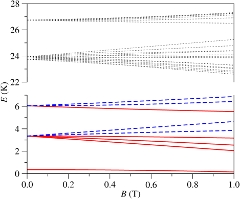
Figure 1:

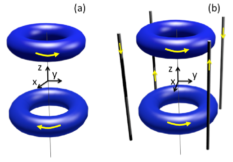
Figure 2:

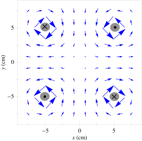
Figure 3:

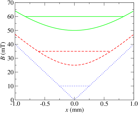
Figure 4:

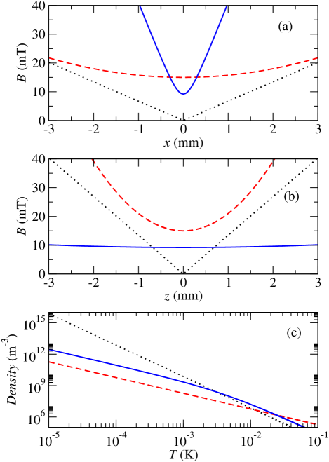
Figure 5: