Gamma-ray constraints on dark-matter annihilation
to electroweak gauge and Higgs bosons

Abstract

Dark-matter annihilation into electroweak gauge and Higgs bosons results in $\gamma$-ray emission. We use observational upper limits on the fluxes of both line and continuum $\gamma$-rays from the Milky Way Galactic Center and from Milky Way dwarf companion galaxies to set exclusion limits on allowed dark-matter masses. (Generally, Galactic Center $\gamma$-ray line search limits from the Fermi-LAT and the H.E.S.S. experiments are most restrictive.) Our limits apply under the following assumptions: a) the dark matter species is a cold thermal relic with present mass density equal to the measured dark-matter density of the universe; b) dark-matter annihilation to standard-model particles is described in the non-relativistic limit by a single effective operator ${\cal O}\propto J_{DM}\cdot J_{SM}$, where $J_{DM}$ is a standard-model singlet current consisting of dark-matter fields (Dirac fermions or complex scalars), and $J_{SM}$ is a standard-model singlet current consisting of electroweak gauge and Higgs bosons; and c) the dark-matter mass is in the range 5 GeV to 20 TeV. We consider, in turn, the 34 possible operators with mass dimension 8 or lower with non-zero $s$-wave annihilation channels satisfying the above assumptions. Our limits are presented in a large number of figures, one for each of the 34 possible operators; these limits can be grouped into 13 classes determined by the field content and structure of the operators. We also identify three classes of operators (coupling to the Higgs and $SU(2)_{L}$ gauge bosons) that can supply a 130 GeV line with the desired strength to fit the putative line signal in Fermi data, while saturating the relic density and satisfying all other indirect constraints we consider.

I Introduction

Until the nature of dark matter and dark energy is understood, the remarkable success of the standard model of cosmology in accounting for observations will be less than completely satisfying. The most popular explanation for dark matter (DM) is that it is an early-universe relic in the form of an undiscovered, electrically neutral, non-hadronic, stable species of elementary particle. Of the many possibilities for the origin and nature of this purported new elementary particle, one that is particularly amenable to experimental and observational tests is that the new species is a cold thermal relic.

The cold thermal relic scenario assumes that the new particle species was established in local thermodynamic equilibrium when the temperature of the universe was larger than the mass of the particle. The processes establishing the initial equilibrium abundance are assumed to be the annihilation of the new species into standard-model (SM) particles and the production of the new species from initial SM-particle states. Then, as the universe cools to temperatures below the dark-matter mass, the relative abundance of the new species (relative to, say, the entropy density) “freezes out” as the rate of processes keeping the species in equilibrium falls below the expansion rate of the universe. The relative freeze-out abundance, and therefore the present mass density, is thus related to the cross section of dark-matter annihilation into SM particles.

Observationally the ratio of the present average dark-matter mass density to the critical density is well determined to be $\Omega_{DM}h^{2}\simeq 0.12$ Ade et al. (2013). The requirement that this mass density is saturated by the mass density of the cold thermal relic determines the annihilation cross section (and, in some cases, also the mass) of the new species. Since the mass and annihilation cross section required are both of order the weak scale, the cold thermal relic is known as a weakly interacting massive particle, or WIMP.

A key feature of the WIMP hypothesis is the requisite DM–SM coupling, and its close relationship to the present dark-matter mass density. Indeed, it is knowledge of the coupling of WIMPs to SM particles that provides the experimental and observational avenues that could lead to the discovery of the nature of the dark matter: detection of WIMPs through their present-day scattering with SM particles ($\mathrm{WIMP}+\mathrm{SM}\rightarrow\mathrm{WIMP}+\mathrm{SM}$), known as “direct detection”; detection of WIMPs through the observation of the present-day annihilation products of WIMPs into SM particles ($\mathrm{WIMP}+\mathrm{WIMP}\rightarrow\mathrm{SM}+\mathrm{SM}$), known as “indirect detection”; and production and detection of WIMPs at particle colliders ($\mathrm{SM}+\mathrm{SM}\rightarrow\mathrm{WIMP}+\mathrm{WIMP}$).

While the WIMP–SM coupling is a common refrain in all WIMP scenarios, there are a tremendous number of variations on this theme. One possibility is that the WIMP is not the only new particle at the weak scale, and these additional new particles play a crucial role in the annihilation, production, or scattering of WIMPs. In the other limit that the masses of any additional new particles are much greater than momenta in the processes of interest, we can integrate out the additional states and describe the WIMP–SM interaction in terms of an effective field theory (EFT). We will work in this “Maverick” limit.

Even within this context there are a large number of possibilities. The first study assumed that the WIMP couples to SM fermions Beltran et al. (2009). In this case direct detection Beltran et al. (2009) and collider searches Beltran et al. (2010); Goodman et al. (2011, 2010); Fox et al. (2012a, b); Rajaraman et al. (2011); Fox et al. (2011, 2012a); Aad et al. (2012); ATL (2012); Chatrchyan et al. (2012); CMS (2013); Lin et al. (2013) offer the best possibility for testing the models.

Another class of possibilities which admits an EFT description is that dark matter couples to (SM) diboson final states of electroweak gauge and Higgs bosons Chen et al. (2013). Here we consider DM–SM couplings of the form $\Lambda^{-n}J_{DM}\cdot J_{SM}$, where $J_{DM}$ is a standard-model-singlet current consisting of dark-matter fields (assuming Dirac fermions or complex scalars), $J_{SM}$ is a standard-model-singlet current consisting of electroweak gauge and Higgs bosons, and $\Lambda$ is the mass scale (“suppression scale”) of the effective field theory. Moreover, we only consider the case that the dark-matter field is a singlet under $SU(2)_{L}\times U(1)_{Y}$.

Chen et al. (2013) (hereafter “CKW”) listed all such operators with diboson final states up to mass dimension 8, and presented detailed calculations of dark-matter annihilation cross sections to all possible final states, including $\gamma\gamma$, $\gamma Z$, $\gamma h$, $ZZ$, $Zh$, $W^{+}W^{-}$, $hh$ and $\bar{f}f$. In order to consistently describe this list of possible channels, they required $J_{SM}$ to be invariant under $SU(2)_{L}\times U(1)_{Y}$. Of the 50 such operators they enumerated, they demonstrated that 34 of them have at least one $s$-wave annihilation channel for at least some values of the dark-matter mass $M$, and hence could produce a detectable indirect detection signal. ($p$-wave annihilation is suppressed by $v^{2}\sim 10^{-6}$ relative to $s$-wave annihilation at the present epoch.)

DM annihilation to diboson final states leads in all cases to prompt production of $\gamma$-rays, including possibly monochromatic photons. This leads naturally to the prospect that there could be non-negligible present-day DM-annihilation photon fluxes emanating from regions of high dark-matter density: in particular, from the Galactic Center of the Milky Way, or from Milky Way companion dwarf galaxies. The aim of the present work is to utilize the experimentally measured upper bounds on these photon fluxes to place constraints on those EFT operators which have non-negligible $s$-wave annihilation cross sections.

More precisely, considering in turn each of the 34 EFT operators mentioned above, we will derive constraints on the allowed dark-matter mass $M$ assuming that the WIMP annihilates only via the operator in question, and that it is a cold thermal relic which accounts for 100% of the measured DM density in the universe. We use the following analyses to set limits: the Galactic Center (GC) Fermi-LAT line-search limits for photon energies 5 to 300 GeV presented in Ref. Ackermann et al. (2013a); the H.E.S.S. GC line-search limits for photon energies 500 GeV to 20 TeV presented in Ref. Abramowski et al. (2013); the analysis of the GC Fermi-LAT inclusive flux limits for photon energies 0.1 to 100 GeV presented in Hooper et al. (2012); and the Fermi-LAT Milky Way dwarf companion limits for photon energies 0.2 to 100 GeV presented in Ref. Ackermann et al. (2011). In addition, many of the operators have one or more annihilation modes with monochromatic photons; we investigate whether these operators can fit the possible $\gamma$-ray line at $E_{\gamma}\approx$ 130 GeV observed in the Fermi-LAT data, as first reported in Weniger (2012). In cases where a reasonable fit to the photon line is possible, we apply the limits presented in Cohen et al. (2012) for the ratio of continuum-to-line emission for DM masses of 125 to 150 GeV.

Our limits are presented in a large number of figures, one for each of the 34 possible operators, in Sec. IV. The limits on the operators depend on available annihilation channels, which are determined by both the field content and structure of the operator, and the dark-matter mass. Based on qualitative differences in their predicted indirect detection signals, we group the operators into 13 classes, which are summarized in Table 3 in Sec. V. Overall, we observe that line searches give the most constraining limits for operators whose indirect detection signal has a significant contribution from one or more photon lines. Other limits, such as that from the continuum photons, are weaker but still useful for lighter dark matter masses. Although some operators are quite severely constrained by the photon fluxes over a large region of parameter space, for the majority of the operators we find that most of the parameter space is still open or is only weakly constrained. Among all the operators considered here, we have also identified three classes which can simultaneously give the correct thermal relic abundance, account for the potential 130 GeV line signal, and be consistent with all the constraints from indirect searches which we have considered. More importantly, our results demonstrate that it is possible to set interesting limits on dark matter annihilations by combining various channels. They can also be used to infer additional predictions and learn about the nature of dark matter if a signal is observed in a particular channel.

We also identify an interesting effect for fermion DM coupling via pseudo-vector $J_{DM}$ where the $p$-wave annihilation cross section is enhanced (relative to the $s$-wave) at large $M$ by coupling to the longitudinal mode of a massive vector boson in the final state. This actually has the effect, since saturation of $\Omega h^{2}$ fixes the total cross section at freeze-out, of suppressing the $s$-wave (i.e. present-day) annihilation cross section thereby alleviating constraints on these operators for large $M$.

Since there have been many works that discuss indirect-detection limits, it is appropriate for us to discuss why our analysis is new. Our starting point is the assumption that low-energy WIMP annihilation processes can be described by an effective field theory with the assumptions discussed above. Working within that framework, for each possible operator, the full $SU(2)_{L}\times U(1)_{Y}$ gauge invariance of $J_{SM}$ forces us to consider all possible final states. Moreover, the requirement of gauge invariance determines the relative strength of possible annihilation channels. We expect the existence of multiple annihilation channels to offer much more discriminating power in the analysis. A related earlier work is Cotta et al. (2012), where a more limited set of operators (without including the Higgs and without requiring full $SU(2)_{L}$ gauge invariance) was considered. In addition, some of these operators have been discussed in Refs. Weiner and Yavin (2012, 2013); Rajaraman et al. (2013), with an emphasis on explaining the 130 GeV line as well as a possible additional line at around 114 GeV Rajaraman et al. (2012).

We emphasize that, in general, the EFT approach must be taken with some caution; the case at hand is no exception. Every relevant process involving WIMPs has a characteristic scale for the momentum transfer, and the accuracy of the EFT approach can be measured by the comparison between this scale and the suppression scale of the effective operators Shoemaker and Vecchi (2012); Busoni et al. (2013); Buchmueller et al. (2013). In this sense, the approach would become less accurate in describing the freeze-out and present-day DM annihilation if the suppression scale is close to the dark-matter mass. As it happens, in order to give the correct thermal relic abundances, some of the operators we study are forced to have $\Lambda\sim M$ and, in principle, one therefore needs to delve into possible UV completions in these cases. This caveat notwithstanding, given the large number of possible operators and final states we consider, we find it useful to use ‘naïvely’ the effective operator approach to give rough estimates. Considering the large systematic astrophysical uncertainties in the indirect detection measurements we utilize, a more accurate description within a UV complete model would not change our conclusions qualitatively.

The remainder of this paper is arranged as follows. In Sec. II we discuss some theoretical background on the WIMP relic density, DM halo profiles, annihilation photon fluxes, and continuum photon spectra from various DM annihilation channels. In Sec. III we discuss the individual experimental limits we have worked with, summarizing how they were obtained and how we have interpreted them. The large number of plots giving the results of our work are given in Figs. 4 to 37 in Sec. IV. We discuss the results and conclude in Sec. V. There are a number of appendices: Appendix A discusses in some detail the contribution to the photon spectrum due to inverse Compton scattering. Appendix B summarizes the magnitude of other systematic errors we did not take into account. Finally, Appendix C discusses some further analysis we have performed on one of the literature sources we have consulted for the case where there are two partially resolved lines in the photon spectrum.

II Preliminaries

II.1 Relic density

It is a well known phenomenon Kolb and Turner (1994) that a massive particle species capable of annihilation into less massive species, and which is initially in thermodynamic equilibrium in the early universe, cannot maintain an equilibrium abundance to arbitrarily low temperature as the universe expands. Eventually, annihilations become too infrequent owing to the dilution of the particles in the expanding volume of the universe, and creation of a pair of the new particle species becomes rare because it becomes exponentially rare to have collisions with sufficient center-of-mass energy. This leads to a “freeze out” of the abundance of the new particle species to some relic abundance. We shall assume that the measured average dark matter density of the universe, $\Omega_{DM}h^{2}=0.12$ Ade et al. (2013), is entirely ascribable to the WIMP, which we will assume to be either a complex scalar or a Dirac fermion.

The phenomenon of thermal freeze-out is well described by the Boltzmann equation Kolb and Turner (1994), and given the necessary initial data and annihilation cross sections as a function of temperature, one can simply solve this equation numerically to find the relic abundance. There does, however, exist an approximate method which has the benefit of expressing the relic abundance in closed form. We shall assume that a non-relativistic approximation to the annihilation cross section can be written in the form $\langle\sigma v\rangle_{NR}=a+bv^{2}$, where $a$ and $b$ are constants, $v^{2}=6T/M$, and $\langle\cdots\rangle$ indicates the thermal average. The DM relic density can then be given to ca. 5% accuracy by Kolb and Turner (1994); Chen et al. (2013)

$$\Omega_{DM}h^{2} =\frac{1.04\times 10^{9}\text{GeV}^{-1}}{M_{\text{Pl}}\sqrt{g_{*}(x_{F})}}\frac{x_{F}}{(a+3b/x_{F})}\times\left\{\begin{array}[]{ll}1&\text{for self-conjugate DM}\\ 2&\text{for non-self-conjugate DM}\end{array}\right.,$$ (1c)

$$x_{F}\equiv\frac{M}{T_{F}}=\ln\left[c(c+2)g\sqrt{\frac{45}{8}}\frac{MM_{\text{Pl}}}{2\pi^{3}\sqrt{g_{*}(x_{F})}}\frac{a+6b/x_{F}}{\sqrt{x_{F}}}\right],$$ (1d)

where $x_{F}=M/T_{F}\sim\mathcal{O}(20)$ with $T_{F}$ the freeze-out temperature Kolb and Turner (1994), $M$ is the WIMP mass, $M_{\text{Pl}}=1.22\times 10^{19}$ GeV is the Planck mass, the numerical parameter $c$ is chosen such that $c(c+2)=1$, and the number of relativistic degrees of freedom at freeze-out is taken to be $g_{*}(x_{F})=106$ Chen et al. (2013); Kolb and Turner (1994). For real or complex scalar DM, $g=1$, and for both Majorana and Dirac fermion DM, $g=2$. For the results in this paper we will assume non-self-conjugate DM, since some of the operators under consideration vanish for self-conjugate DM.

Working in an EFT framework and assuming that the DM annihilation proceeds through only one EFT operator $\mathcal{O}(x)$ of mass-dimension $d$, the term in the Lagrangian responsible for the annihilation can be written $\mathcal{L}(x)\supset\Lambda^{4-d}\mathcal{O}(x)$. It then follows that $\langle\sigma v\rangle$ is proportional to $\Lambda^{2(4-d)}$. Thus, for a given operator, $\Omega_{DM}h^{2}$ is a function of $M$ and $\Lambda$. Since we assume the particle is a WIMP accounting for 100% of the observed DM in the universe, for a given mass $M$ we shall numerically solve Eq. (1) for the EFT scale parameter $\Lambda$ to satisfy the relation $\Omega_{DM}h^{2}=0.12$. This requirement implies that for each operator, for a given mass $M$ there are no free parameters in the low-energy annihilation cross section.

II.2 DM Density Profiles

Although thermal freeze-out is predicated on the effective shutoff of annihilation in the early universe, this does not imply that WIMP annihilation remains negligible for the remainder of the evolution of the universe. Structure formation leads to large local densities of both baryonic and dark matter, and this obviously implies that the annihilation rate $\Gamma\sim n\sigma v$ may again become large enough for detectable levels of annihilation to occur in regions such as the Milky Way Galactic Center (GC), or in the dark-matter-rich Milky Way dwarf companion galaxies.

Understanding the spatial distribution $\rho(r)=Mn(r)$ of the DM mass density in the relevant regions is important in the interpretation of any putative annihilation signal. The $N$-body simulation community is actively studying this, but there is as yet no consensus in the literature for the exact form this so-called halo profile takes in galaxies such as our own. Consequently, it is conventional to quote all results assuming a number of different profiles. For constraints from Milky Way GC observations, we will utilize the (generalized) Navarro-Frenk-White, the Einasto, and the Isothermal profiles Iocco et al. (2011); Ackermann et al. (2013a, 2012a); Abramowski et al. (2013); Hooper et al. (2012).

Table 1: Milky-Way DM halo profile normalizations. We utilize a band of normalizations corresponding to the central value of $\rho_{\odot}\pm 2\sigma$ limits consistent with microlensing and galactic rotational velocities given in Iocco et al. (2011). For generalized NFW and Einasto profiles, we assume $r_{s}=20$ kpc, and $r_{\odot}=8$ kpc, and take the $\rho_{\odot}$ values from Iocco et al. (2011); for the Isothermal profile we assume $r_{s}=5$ kpc, and $r_{\odot}=8$ kpc, and use representative values for $\rho_{\odot}$.

	$2\sigma$ lower limit on $\rho_{\odot}$ [GeV/cm3]	Central value of $\rho_{\odot}$ [GeV/cm3]	$2\sigma$ upper limit on $\rho_{\odot}$ [GeV/cm3]
	generalized NFW
$\gamma=1.0$	$0.28$	0.40	0.54
$\gamma=1.2$	$0.25$	0.36	0.48
$\gamma=1.3$	$0.235$	0.34	0.45
	Einasto
$\alpha=0.17$	$0.245$	0.36	0.57
	Isothermal
	$0.30$	0.40	0.50

Table 2: Summary of the main sources used to compute cross section limits, with corresponding choices of DM halo profile normalizations and $J$ factors where applicable. [The $J$ factor is defined in Eq. (6d).] If no value for a parameter was explicitly stated in a given reference, we indicate why we have assumed the indicated value. The region of interest (ROI) used in the analysis is indicated in parentheses following the notation of the source referenced. Further details in each case can be found in the referenced section number. In the final column we give the rescaling factor $K$ applied in order to map published limits onto the halo profiles and normalizations given in Table 1; further details on the rescaling are given in Sec. II.3.1. For the most part the rescaling comes from scaling $J$ factors with $\rho_{\odot}^{2}$. The only exception is the isothermal case used by Weniger, where there is a significant difference in $r_{s}$ that affects the $J$ factor by a factor of 2.

Profile (ROI)	$\gamma$ or $\alpha$	$r_{s}$ [kpc]	$r_{\odot}$ [kpc]	$\rho_{\odot}$ [GeV/cm3]	$J$ factor [$10^{21}$GeV2/cm5]	$K$
Fermi line search, Ackermann et al. (2013a) — Sec. III.1
NFWc (R3)	$\gamma=1.3$	$20.0$	$8.2$	$0.4$	$13.9$	$0.689$
NFW (R41)	$\gamma=1.0$	$20.0$	$8.2\textsuperscript{\ref{ftnote1}}$	$0.4$	$8.48$	$0.960$
Einasto (R16)	$\alpha=0.17$	$20.0$	$8.2\textsuperscript{\ref{ftnote1}}$	$0.4$	$8.53$	$0.770$
Isothermal (R90)	—	$5.0$	$8.2\textsuperscript{\ref{ftnote1}}$	$0.4$	$6.94$	$0.962$
H.E.S.S. line search, Abramowski et al. (2013) — Sec. III.2
NFWc	$\gamma=1.3$	$20.0$	$8.0$	$0.42$	$22.1$	$0.655$
NFW	$\gamma=1.0$	$20.0$	$8.0$	$0.42$	$4.37\textsuperscript{\ref{ftnote3}}$	$0.907$
Einasto	$\alpha=0.17$	$20.0$	$8.0$	$0.42$	$2.43\textsuperscript{\ref{ftnote3}}$	$0.735$
Isothermal	—	$5.0$	$8.0$	$0.42$	$0.312\textsuperscript{\ref{ftnote3}}$	$0.907$
Template-based analysis, Hooper et al. (2012) — Sec. III.3
NFWc	$\gamma=1.2$	$20.0$	$8.0$	$0.25$	—	$2.07$
NFW	$\gamma=1.0$	$20.0$	$8.0\textsuperscript{\ref{ftnote2}}$	$0.28$	—	$2.04$
Einasto	$\alpha=0.17$	$20.0$	$8.0\textsuperscript{\ref{ftnote2}}$	$0.25$	—	$2.07$
Line search based on Fermi data, Weniger (2012) — Sec. III.6
NFWc (Reg4)	$\gamma=1.3$	$20.0$	$8.5$	$0.4$	—	$0.644$
NFW (Reg4)	$\gamma=1.0$	$20.0$	$8.5$	$0.4$	—	$0.890$
Einasto (Reg4)	$\alpha=0.17$	$20.0$	$8.5$	$0.4$	—	$0.715$
Isothermal (Reg4)	—	$3.5$	$8.5$	$0.4$	—	$0.443$

The generalized Navarro-Frenk-White (NFW) DM density profile is given by Iocco et al. (2011)

$$\rho(r;\gamma) =\frac{\rho_{0}}{\left(r/r_{s}\right)^{\gamma}\left(1+r/r_{s}\right)^{3-\gamma}},$$ (2)

where the scale parameter is chosen to be $r_{s}=20$ kpc. The parameter $\gamma$ controls the central slope of the profile: $\gamma=1$ for the canonical NFW profile, while $\gamma>1$ defines a profile with a steeper central region (where $\rho\sim r^{-\gamma}$), known as a contracted profile (NFWc) which may arise due to gravitational interactions between the dark and baryonic matter as the latter cools during galaxy formation Gnedin et al. . In either case, the profile is peaked toward $r=0$ and “cuspy.” The overall scale $\rho_{0}$ is chosen for galactic measurements such that the local (in the vicinity of the Sun) DM density $\rho(r_{\odot})\equiv\rho_{\odot}$ takes some desired value (see Table 1), while for extragalactic (dwarf) measurements, $\rho_{0}$ is chosen to obtain the correct observed stellar rotational velocities Ackermann et al. (2011).

The Einasto profile is given by Iocco et al. (2011)

$$\rho(r) =\rho_{0}\exp\left\{-\frac{2}{\alpha}\left[\left(\frac{r}{r_{s}}\right)^{\alpha}-1\right]\right\}$$ (3)

where the scale parameter is chosen to be $r_{s}=20$ kpc. In line with large-scale numerical simulations, the parameter $\alpha=0.17$ is used. This profile is cuspy. Overall normalizations are chosen similarly to the NFW profile; see Table 1.

The Isothermal profile is given by Iocco et al. (2011)

$$\rho(r) =\frac{\rho_{0}}{1+(r/r_{s})^{2}}$$ (4)

where the scale-parameter $r_{s}=5$ kpc is chosen. This profile is known as “cored” since $\rho(r)$ flattens off to a constant value at small $r$. Overall normalizations are again chosen similarly to the NFW profile; see Table 1.

We have scaled all the limits presented in this paper to reflect the halo profile parameters presented in Table 1 (original parameters assumed in the literature are shown in Table 2; see Sec. II.3.1 for more details on the rescaling).

II.3 Annihilation Photon Flux

For all the EFT operators under consideration, the detectable annihilation signal in $\gamma$-rays includes a) one or more monochromatic prompt photon “lines” arising from the direct annihilation DM DM $\rightarrow\gamma X$ where $X$ can be any SM boson consistent with gauge symmetries ($X=\gamma,Z,h$), and/or b) a prompt diffuse continuum photon flux arising from final-state radiation or radiative hadron decay arising when considering various non-photon primary DM annihilation products: DM DM $\rightarrow XY\rightarrow\gamma$’s where $X$ and/or $Y$ is not a photon.

For each particular operator there will be a characteristic per-annihilation differential prompt photon spectrum

$$\frac{dN_{\gamma}(E)}{dE}\equiv\sum_{f}\text{BR}_{f}\left(\frac{dN^{f}_{\gamma}(E)}{dE}\right)$$ (5)

where $\text{BR}_{f}\equiv\sigma\left(\text{DM DM}\rightarrow f\right)/\ \sigma_{\text{total}}$ is the branching ratio for the annihilation mode to final-state $f$, $dN^{f}_{\gamma}(E)/dE$ is the per-annihilation differential prompt photon spectrum for that mode, and the sum runs over all annihilation modes for the operator. Given this spectrum, the differential DM-annihilation prompt photon flux which an experiment would observe at photon energy $E$ is given by Ackermann et al. (2012a)

$$\frac{d\Phi(E)}{dE} =\frac{[\sigma v]_{\text{total}}}{16\pi M^{2}}\ J\ \frac{dN_{\gamma}(E)}{dE}\quad\times\left\{\begin{array}[]{ll}2&\text{for self-conjugate DM}\\ 1&\text{for non-self-conjugate DM}\end{array}\right.$$ (6c)

$$\text{where}~{}~{}~{}~{}J =\int_{\text{LOS-ROI}}\rho^{2}[r(s,l,b)]\ ds\ \cos b\ db\ dl.$$ (6d)

Hereafter we will assume non-self-conjugate DM, i.e., complex scalars and Dirac fermions. In the equation above, $\rho(r)$ is the DM density profile at Galactocentric distance $r$. The astrophysical “$J$ factor” [Eq. (6d)] is computed by integrating the squared DM density along the line of sight (LOS) from the Earth, and over the relevant Galactic lat/long coordinates. The integral over $b$ and $l$ defines a search region of interest (ROI). A point observed at LOS distance $s$ at lat/long coordinates $(l,b)$ has Galactocentric distance $r=\left(s^{2}+r_{\odot}^{2}-2sr_{\odot}\cos l\cos b\right)^{1/2}$ where $r_{\odot}$ is the Sun–GC distance. We will always take $r_{\odot}=8$ kpc Iocco et al. (2011). Finally note that the polar angle $\theta$ from the GC satisfies $\cos\theta=\cos l\cos b$.

It is our aim to place upper limits on the non-relativistic cross sections $\sigma v$ using experimentally determined upper limits on such photon fluxes.

II.3.1 Profile rescaling

The constraints derived in this paper draw on published gamma-ray line searches and limits on diffuse emission from several sources, each of which employ different assumptions for Milky Way halo profiles. We give the parameters used by these references in Table 2. For consistency, however, we would like to derive limits for a single set of halo profile parameters (given in Table 1).

The difference in halo profiles is encapsulated in the $J$ factor; typically we wish to take some given $J$ factor from the literature (using some values of $r_{\odot}$, $\rho_{\odot}$ and/or $r_{s}$) and rescale it to values of $r_{\odot}^{\prime}$, $\rho_{\odot}^{\prime}$ and/or $r_{s}^{\prime}$ that are our choices. All other things being equal, the limit for $\sigma v\propto 1/J$, so the cross section limit that would be set with the new set of halo parameters is

$$[\sigma v]^{\prime}=\frac{J}{J^{\prime}}\ [\sigma v]\equiv\ \frac{[\sigma v]}{K}.$$ (7)

Here $J^{\prime}$ is the $J$ factor computed with the set of parameters we wish to use and $J$ is the $J$ factor we compute using the parameters in the literature. We thus rescale the published limits by the factor $K$ (see Table 2).

We find that scaling the $J$ factors with $\rho_{\odot}^{2}$ accounts for most of the difference in the halo profile normalizations. This is primarily because the variation in $\rho_{\odot}$ values used in the literature is large (up to 40$\%$), while the variation in the $r_{\odot}$ values is less than 10$\%$, and the $r_{s}$ values are almost uniform. There is only one case where there is a large difference in $r_{s}$; for the isothermal profile for Reg4 of Ref. Weniger (2012) where $r_{s}=3.5\ \text{kpc}\rightarrow 5.0\ \text{kpc}$. In this case the rescaling factor was roughly a factor of 2 smaller than one would have obtained from simply scaling $J$ with $\rho_{\odot}^{2}$, accounting for the fact that the core is less dense when $r_{s}$ is increased.

Note that for the Fermi ROIs, we have computed these rescaling factors without considering point source masking effects which are estimated to impact the $J$ factor by less than about $10\%$. Our justification for this simplification is that the halo profiles are smooth away from $r=0$, so that the ratios $J^{\prime}/J$ computed with or without point-source masking being considered should be very nearly equal (certainly much closer than 10$\%$).

We also point out that the rescaling of the Reg4 values from Ref. Weniger (2012) is appropriate even though the ROIs in that reference were chosen based on an expected signal/background analysis with a specific profile in mind. Weniger (2012) reports cross section results from each such ROI choice assuming a number of different profiles in the conversion from flux to cross section while holding the ROI fixed, and it is only these flux-to-cross-section conversions we are rescaling. Similarly, the ROIs in Ref. Ackermann et al. (2013a) were chosen based on an expected signal/background analysis; but again, we are simply holding their chosen ROI, and hence fluxes, fixed and are only rescaling the flux-to-cross-section conversion.

II.4 Photon Spectra

In the models we study, dark matter annihilation produces primary electroweak gauge bosons ($\gamma$, $Z$, $W^{\pm}$), higgs bosons, or fermions. In addition to primary photons, the subsequent shower and hadronization of final states will produce abundant hadrons, giving rise to additional prompt photons dominantly through decay of neutral pions $\pi^{0}\rightarrow\gamma\gamma$. To extract cross section upper limits from the measured flux upper limits requires knowledge of this per-annihilation prompt photon spectrum, see Eq. (6c). Here we summarize the physics of prompt photon production from DM annihilation.

We begin our discussion with monochromatic photons. The $\gamma\gamma$ and $\gamma h$ final states give rise to photon lines. The contribution to the photon spectrum is a delta function: $dN(E)/dE=N_{\gamma}\delta(E-\widetilde{E}_{\gamma})$, where simple kinematics gives $\widetilde{E}_{\gamma}=M-m_{X}^{2}/4M$ for a $\gamma X$ final state, and $N_{\gamma}$ counts the number of monochromatic photons in the decay mode ($N_{\gamma}=2$ for the $\gamma\gamma$ annihilation modes and $N_{\gamma}=1$ otherwise). The photon line from a $\gamma Z$ annihilation mode is similarly peaked at $E_{\gamma}=M-m_{Z}^{2}/4M$, but obviously has a finite width due to the finite width of the $Z$. The width of the line will be relevant to our discussion of experimental constraints later and is shown in Fig. 1.

For annihilation modes $W^{+}W^{-},\ ZZ,\ Zh,\ hh,\ f\bar{f},\ \gamma h,\ \mathrm{and}\ \gamma Z$, there is also a continuum prompt photon spectrum. We employ Pythia 8.176 Sjöstrand et al. (2007) to perform the shower and hadronization (and hadron decay) to obtain the photon spectra. Following Ref. Cirelli et al. (2010), we create a fictitious spin-1 resonance at $m=2M$ with a width of 1 GeV, which we populate using fictitious $e^{+}e^{-}$ colliding beams free of initial-state radiation at $\sqrt{s}=2M$. We set by hand the resonance decay channels to be, in turn, 100% to each of the desired primary final states, and the per-annihilation differential photon spectra are computed by correctly normalizing the histogrammed photon energies from 10⁵ simulated annihilations per mass point per primary final state.

Good agreement is found between these computed Pythia spectra and a set of spectra from Cirelli et al. (2010) for DM masses below 300 GeV. For larger DM masses, the effects of electroweak (EW) final-state radiation (FSR) of $W$s and $Z$s (which are not included in the Pythia shower) can significantly alter the spectra at low $E_{\gamma}$ Ciafaloni et al. (2010); Cirelli et al. (2010); these effects have been included in the spectra in Cirelli et al. (2010). However, we shall see below that we will be primarily interested in the spectrum for $E_{\gamma}\in[10,100]$ GeV at large DM mass. In this photon energy range, the EW corrections are unimportant for $M\lesssim 1$ TeV except for primary final states containing charged leptons, which in any event give rise to about an order of magnitude fewer photons per annihilation compared to other channels. Furthermore, the branching fraction for annihilation to leptonic final states in particular, and fermionic final states more generally, is subdominant at large $M$ (see the result plots in Sec. IV), with the exception of operator XX-1 where all annihilations are mediated through an $s$-channel $Z$ or $\gamma$. Therefore, since the error of neglecting the EW FSR is small, and since the necessary spectra are not all available in Cirelli et al. (2010), we have chosen for the sake of uniformity to use the Pythia spectra which we have computed rather than attempting to use the corrected spectra from Cirelli et al. (2010).

II.4.1 Qualitative understanding of the shape of the photon spectra

The shape, and in particular the DM-mass dependence, of the continuum photon spectrum differs qualitatively depending on whether the primary final states are leptonic, non-leptonic and color neutral, or colored. We consider illustrative cases for the latter two: annihilation to $W^{+}W^{-}$ and annihilation to $\bar{b}b$ (light $q\bar{q}$ modes are qualitatively similar), and comment on the leptonic modes.

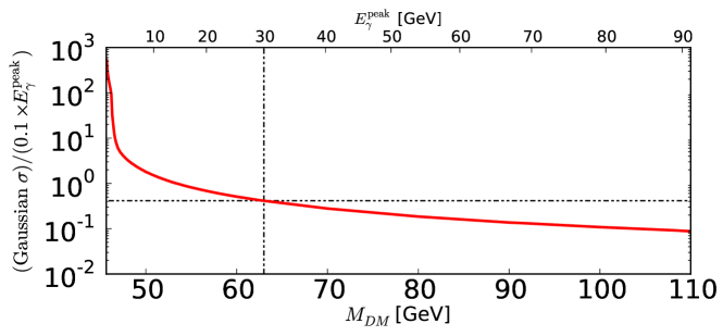
Figure 1: The Gaussian standard deviation of the photon line arising from the $\gamma Z$ primary final state as a function of DM mass, expressed in units of $0.1\times E_{\gamma}$, approximately the Fermi-LAT energy resolution (68% containment half-width). The line-width is large with respect to the resolution for DM masses less than about $60$ GeV; we only set limits on photon lines from $\gamma Z$ for $M>63$ GeV ($E_{\gamma}>30$ GeV), as discussed in the text. The standard deviation here has been extracted by fitting a Gaussian to photon line shapes computed with Pythia (this provides a good fit to the central region of the peak but mismodels the tails).

Consider first the $WW$ case. In Fig. 2 we plot the photon spectrum decomposed into photons from $\pi^{0}$ decay and those from final state radiation (FSR) of charged leptons (omitting other hadronic-decay photons for clarity). For $E_{\gamma}\gtrsim 1$ MeV, the production mechanism is dominantly due to pion decay. The strongest continuum $\gamma$-ray constraints are for energies from 0.1 GeV to 100 GeV, so we will always be in the regime where the behavior of the photon spectrum from diboson annihilation channels is dominated by photons from $\pi^{0}\rightarrow\gamma\gamma$. Meanwhile, the FSR from leptons has a spectrum that goes like $dN_{\gamma}/dE_{\gamma}\sim E_{\gamma}^{-1}$ and is subdominant for $E_{\gamma}\gtrsim 1$ MeV.

Since $W$ is color neutral, the spectrum and multiplicity of photons is determined by the independent decay and shower of each $W$, boosted into the center of mass frame of the annihilation. As $M$ increases, the $W$s are increasingly boosted and the decay products also become more energetic while the multiplicity (namely the pion yield) remains roughly constant. We can observe this in the shifting of the photon spectrum in Fig. 2 to higher energies. Furthermore, this migration to higher energy decay products, while the yield remains constant, leads to the effect that as $M$ increases there is a decrease in the number of photons produced at low energy. This can also be observed in e.g., Panel B of Fig. 6, where for $M>100$ GeV where the $WW$ final state dominates, there is a decrease in the photon spectrum around $E_{\gamma}\sim 0.1$ GeV as $M$ increases.

Since most of the operators considered here have annihilation modes into gauge bosons or higgs, the mass dependence of the $\gamma$-ray spectra has similar behavior to the $WW$ case, modulo the effect of changing branching fractions. Some operators which have only diboson annihilation modes also show first an increase in the low-energy photon spectrum with increasing $M$ below or around a hundred GeV before the decrease discussed above sets in. This has less to do with the intrinsic photon spectrum from each annihilation mode and more to do with the branching fractions for each mode. If the $\gamma\gamma$ mode is present, then the branching fraction to $\gamma Z$ starts off small around $M\sim m_{Z}/2$ and rapidly increases with $M$ giving the observed increase in the continuum spectrum (e.g., Operator VI-1 in Fig. 4 of Sec. IV). In this case, there may be a $WW$ or $ZZ$ mode entering once $M$ gets to $m_{W,Z}$, which results in a further increase since the spectra are normalized per-annihilation and twice as many $W/Z$s per annihilation gives twice as many photons per annihilation (the $W$ and $Z$ intrinsic photon spectra are almost identical, modulo kinematic effects). For $M$ above a (few) hundred GeV, the low-energy spectrum begins to decrease again as per the discussion in the previous paragraph. Explanations of a similar nature are possible for cases where other mixtures of diboson annihilation modes are present.

For annihilation to $b\bar{b}$, shown in Fig. 2, the dominant photon-production mechanism is still neutral pion decay, but the same qualitative picture does not obtain: there is a significant increase in the pion yield with increasing $M$ because in this case the initial hard scale for the parton shower is set by $M$ and so the number of FSR gluons and other strongly interacting partons produced in the shower increases significantly as the DM mass increases. Therefore, although the average pion energy does increase, the increase in the pion yield at the same time means that the pion yield at low energies actually slowly increases as $M$ increases; the photon yield thus shows a similar increasing trend. This is evident in the slow overall monotonic increase in the spectrum as $M$ increases for Operator XX-1 shown in Fig. 37. (For the other operators considered here, this behavior gets cut off near $M\sim 100$ GeV since the branching fraction to quarks typically becomes subdominant once diboson annihilation modes become kinematically allowed.)

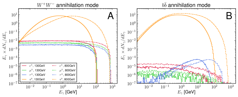
Figure 2: The photon spectrum arising from DM annihilation, decomposed according to the production mechanism of either $\pi^{0}$ decay or final state radiation of charged leptons. We show annihilation to $WW$ (Panel A) and to $b\bar{b}$ (Panel B), for DM mass of 130 GeV and 800 GeV. It is clear that for $E_{\gamma}\gtrsim 1$ MeV, $\pi^{0}$ decay dominates the spectrum. In the case of the $WW$ final state, the shift of the pions to higher energies reflects the increasing boost of each $W$ (and thus of its decay products). For the $b\bar{b}$ final state, the yield of pions increases over the entire energy range of interest. We have omitted the spectra from other hadronic decay modes for clarity.

Finally, for annihilation to charged leptons, the dominant photon production mechanism is direct final-state photon radiation from the leptons. This spectrum falls roughly as $E_{\gamma}^{-1}$ over most of the energy range with a high-energy kinematic cutoff for the photon spectrum at $M$, while the normalization of the photon spectrum grows slowly as $M$ increases. Again however, with the exception of operator XX-1 already noted above, fermionic final states tend to have rapidly falling branching fractions once on-shell diboson final states become kinematically allowed as $M$ increases, so the increase in the spectrum at low $E_{\gamma}\sim 0.1$ GeV is cut off around $M\sim 100$ GeV.

III Limits

In this section we discuss the experimental limits used in constraining the effective operators. We consider line searches in gamma-ray data from Fermi-LAT and H.E.S.S., as well as constraints on diffuse gamma-ray emission derived from Fermi-LAT observations of the GC and dwarf galaxies, for which the continuum photon emission is relevant. We describe our methods of extracting limits for the operators, re-interpreting published results for the specific final states and branching ratios of each operator. Our final results are shown in the figures in Sec. IV, along with a universal caption and summary of the constraints on the operators.

III.1 Low-energy line limits: Fermi-LAT

The Fermi-LAT Collaboration Ackermann et al. (2013a) presents 95% confidence level (CL) upper limits (UL) on the flux $\Phi$ of photons from regions on the sky centered on the Galactic Center due to a strictly monochromatic underlying photon line in the photon energy range 5 to 300 GeV. The underlying photon energy $E_{\gamma}$ was scanned across this range, and for each energy they obtained a flux limit by performing a maximum likelihood analysis in which the Fermi-LAT line shape plus a power-law background was fitted to their 3.7-year data over sliding energy ranges $E_{\gamma}\pm 6\sigma_{E}$ where $\sigma_{E}$ is the Fermi-LAT energy resolution (68% containment half-width). The flux limit $\Phi$ they report is the 95% CL UL of the normalization of the line in this fit, multiplied by a factor giving the effective exposure time of the experiment.

The Fermi-LAT search methodology selected a different signal region of interest (ROI) for each of four DM halo profiles (NFW, Einasto, Isothermal, NFWc_γ=1.3) they considered in order to maximize the expected signal-to-background ratio as estimated through Monte Carlo simulations. Thus, they present four distinct flux limits, one for each ROI. These ROIs are denoted R$\alpha$ where $\alpha$ is the angular size of a circle centered on the GC, with the region $|l|>6^{\circ}$ and $|b|<5^{\circ}$ masked; regions around known $\gamma$-ray point sources are also masked for all ROIs except R3 Ackermann et al. (2013a).

We derive constraints on $\sigma v$ from the flux limits presented in Ref. Ackermann et al. (2013a), which are given at discrete $E_{\gamma}$ in the energy range 5 to 300 GeV; we have interpolated (linearly in $\log\Phi$ vs. $E_{\gamma}$) these limits to intermediate energies where necessary. If the underlying photon line arising from a $\gamma X$ final-state mode is monochromatic or monochromatic to an excellent approximation, we could merely use the flux upper limit at $\widetilde{E}_{\gamma}=M-M_{X}^{2}/4M$ combined with Eq. (6d) and the $J$ factors in Ref. Ackermann et al. (2013a) (rescaled per Table 2) to derive limits on $\sigma v$:

$$\left[\sigma v\right]^{95\%\text{ CL UL}}=\Phi^{95\%\text{ CL UL}}(\widetilde{E}_{\gamma})\times\frac{16\pi M^{2}}{JN_{\gamma}},$$ (8)

where $N_{\gamma}$ is the number of photons in the line per annihilation: 2 for $\gamma\gamma$ and 1 otherwise. This is the case for the $\gamma h$ annihilation mode; complications however arise for the $\gamma Z$ and $\gamma\gamma$ modes for the operators we consider.

The photon line arising from $\gamma Z$ annihilation modes has an intrinsic width of order $1$ GeV, which can be significant with respect to the ca. 5-10% Fermi-LAT energy resolution at low energies Ackermann et al. (2012b, 2013a) (see Fig. 1). However, even for a line with intrinsic width of 50% of the Fermi-LAT energy resolution, the resulting observed spectral feature is only expected to be broadened by around 11% after convolution with the Fermi-LAT energy dispersion function. If such a feature were fitted with a line shape derived from the assumption of a purely monochromatic intrinsic line, the number of photons would be underestimated by about 7% (Ref. Ackermann et al. (2013a), App. D2–3) which would set the flux limit correspondingly more stringent than it should. However, this effect is much smaller than both the expected statistical fluctuation (ca. 50%) in the limits set by Ref. Ackermann et al. (2013a) and the uncertainty in the halo profile normalization (a factor of ca. 10; see results) and it is roughly on the same order as other systematic effects (ca. 10%) which are present in the Fermi-LAT analysis and ignored in their flux upper limits Ackermann et al. (2013a). Provided the linewidth is expected to be less than about half the energy resolution, we therefore make no correction for the finite $Z$ width, and merely use the Fermi-LAT flux limits derived under the assumption of a monochromatic intrinsic line in deriving limits on $\left[\sigma v\right]_{\gamma Z}$. To satisfy this linewidth requirement, we follow the older Fermi-LAT line search analysis Ackermann et al. (2012a) and only present limits on $\sigma v$ from the $\gamma Z$ annihilation mode for $E_{\gamma}\geq 30$ GeV, which corresponds to $M\gtrsim 63$ GeV (see also Fig. 1).

There is a significant complication Fan and Reece (2013) in interpreting the flux limits for all the operators with $\gamma\gamma$ annihilation modes: due to their gauge structure, all such operators under consideration also have a $\gamma Z$ annihilation mode which yields a second line at an energy $\delta E=m_{Z}^{2}/4M$ lower than the $\gamma\gamma$ line. Since the unbinned likelihood analysis in Ref. Ackermann et al. (2013a) is sensitive to both shape and normalization of the line spectral feature, this makes the interpretation of the single-line flux limits difficult in the region of DM masses where the two photon lines are separated by an amount of the order of the Fermi-LAT energy resolution. Depending on the WIMP mass, we have adopted a few different techniques to interpret the single-line flux limits for these operators. In all cases, we choose to use the flux limits to set a single limit on the quantity $\left(2\sigma_{\gamma\gamma}+\sigma_{\gamma Z}\right)v$.

III.1.1 $M<$ 63 GeV

This mass range corresponds to $E_{\gamma}\leq 30$ GeV for the $\gamma Z$ channel (when kinematically allowed), so we do not set a $\gamma Z$ line limit in this mass range. We find the 95% CL UL on $\sigma_{\gamma\gamma}v$ using Eq. (8) with the flux at $E_{\gamma}=M$, and use this to set, at each WIMP mass, the limit

$$\left[\left(2\sigma_{\gamma\gamma}+\sigma_{\gamma Z}\right)v\right]^{95\%\text{ CL UL}}=2(\sigma_{\gamma\gamma}v)^{95\%\text{ CL UL}}\left[1+\frac{\sigma_{\gamma Z}v(M)}{2\sigma_{\gamma\gamma}v(M)}\right]$$ (9)

where the cross section ratio in the $[\ \cdots\ ]$ brackets is computed using the analytic expressions in CKW and rescales the $\sigma_{\gamma\gamma}v$ limit to the quantity $\left(2\sigma_{\gamma\gamma}+\sigma_{\gamma Z}\right)v$.

III.1.2 63 GeV $<M<$ 80 GeV

In this mass region, we have two lines which are relatively well separated assuming a 5 to 10% energy resolution for Fermi-LAT Ackermann et al. (2012b). We thus use Eq. (8) to set independent 95% CL UL on $\sigma_{\gamma\gamma}v$ using the flux at $E_{\gamma}=M$, and on $\sigma_{\gamma Z}v$ using the flux at $E_{\gamma}=M-m_{Z}^{2}/4M$. We use these two quantities to set, at each WIMP mass, the limit

$$\left[\left(2\sigma_{\gamma\gamma}+\sigma_{\gamma Z}\right)v\right]^{95\%\text{ CL UL}}=\text{min}\left\{2(\sigma_{\gamma\gamma}v)^{95\%\text{ CL UL}}\left[1+\frac{\sigma_{\gamma Z}v(M)}{2\sigma_{\gamma\gamma}v(M)}\right]\quad,\quad(\sigma_{\gamma Z}v)^{95\%\text{ CL UL}}\left[1+\frac{2\sigma_{\gamma\gamma}v(M)}{\sigma_{\gamma Z}v(M)}\right]\right\}$$ (10)

where the cross section ratios in the $[\ \cdots\ ]$ brackets are computed using the analytic expressions in CKW.

III.1.3 80 GeV $<M<$ 160 GeV

In this intermediate mass region, the spectral feature expected in the Fermi-LAT data corresponding to the two lines will be very broad with respect to the energy resolution, and may be a double-peaked structure depending on the relative strengths of the lines. Such a feature looks very different from the line shape used in the Fermi-LAT line search Ackermann et al. (2013a) and since, as noted above, that analysis was sensitive to the shape of the fitted feature as well as its normalization, we exercise an abundance of caution and do not set any limits on $\sigma v$ in this region. This caution notwithstanding, we do not expect the limits to differ from those at nearby energies by more than a factor of a few. Since a reproduction of the analysis in Ref. Ackermann et al. (2013a) with a different assumed line shape is a task best suited for the experimental collaboration, we would encourage the Fermi-LAT Collaboration to look into setting flux limits for the case where there may be two partially resolved lines present, with some variable ratio of strengths.

III.1.4 160 GeV $<M$

In this mass region, the two lines are sufficiently close that the spectral feature expected in the Fermi-LAT is merely a slightly broadened (width increased by $\lesssim 10$%) line and a single limit can be set on the combined quantity $\left(2\sigma_{\gamma\gamma}+\sigma_{\gamma Z}\right)v$. We do this by using the flux upper limit from Ref. Ackermann et al. (2013a) evaluated at the flux-weighted average energy

$$\bar{E}_{\gamma}=\frac{2\sigma_{\gamma\gamma}v(M)\times M+\sigma_{\gamma Z}v(M)\times\left(M-m_{Z}^{2}/4M\right)}{2\sigma_{\gamma\gamma}v(M)+\sigma_{\gamma Z}v(M)},$$ (11)

where the cross sections here are computed using the analytic expressions in CKW. The limit is set as

$$\left[\left(2\sigma_{\gamma\gamma}+\sigma_{\gamma Z}\right)v\right]^{95\%\text{ CL UL}}=\Phi^{95\%\text{ CL UL}}(\bar{E}_{\gamma})\times\frac{16\pi M^{2}}{J}\ .$$ (12)

III.2 High energy line limits: H.E.S.S.

The H.E.S.S. Collaboration Abramowski et al. (2013) presents 95% confidence level (CL) upper limits (UL) on the photon flux $\Phi$ from a strictly monochromatic photon line in the energy range 500 GeV to 20 TeV. The ROI is a $1^{\circ}$ radius circle centered on the GC, with $|b|<0.3^{\circ}$ excluded. No masking of point sources was performed. Their flux upper limits were extracted by performing a maximum likelihood analysis in which a Gaussian peak (photon line) was fitted along with a parametrized background to 112 hours of data from the H.E.S.S. VHE $\gamma$-ray experiment. The position of the Gaussian peak was scanned over the search energy range (with the standard deviation constrained to be equal to the H.E.S.S. energy resolution; see below), and the Gaussian normalization and background parameters were fitted at each search energy. The line flux limits reported are the 95% CL UL on the fitted Gaussian normalizations.

Flux limits are only presented at discrete $E_{\gamma}$ on the energy range 500 GeV to 20 TeV in Ref. Abramowski et al. (2013); we have interpolated (linearly in $\log\Phi$ vs. $\log E_{\gamma}$) these limits to intermediate energies where necessary. Isothermal limits here are very weak as a consequence of the cored profile and the ROI which is restricted to a very small region near the GC. It was necessary for interpreting the H.E.S.S. limits to compute the $J$ factors defined in Eq. (6d) for the halo profiles of our choice, given in Table 1. We did this for by computing $J$ factors for the parameters used in the publication (see Table 2) and then rescaling the resulting $J$ factors as necessary, as discussed in Sec. II.3.1.

Additionally, in computing cross section limits from the fluxes, we neglected the small shift in the photon line position for final states involving a massive particle (the largest this shift gets is about 7 GeV for the $\gamma h$ line at $M=500$ GeV) and have simply evaluated all limits assuming $E_{\gamma}=M$. Furthermore, since the H.E.S.S. energy resolution is 17% at 500 GeV, dropping to 11% at 10 TeV Abramowski et al. (2013), it is always a good approximation to combine the unresolved $\gamma\gamma$ and $\gamma Z$ lines into a single spectral feature to derive combined limits on $(2\sigma_{\gamma\gamma}+\sigma_{\gamma Z})v$ for all the operators with both $\gamma\gamma$ and $\gamma Z$ annihilation modes. The width of the photon line from $\gamma Z$ has no significant effect here.

To summarize, we derived cross section limits from the H.E.S.S. flux upper limits using, as appropriate,

$$\left.\begin{array}[]{rrr}\left[\left(2\sigma_{\gamma\gamma}+\sigma_{\gamma Z}\right)v\right]^{95\%\text{ CL UL}}\\ \left[\sigma_{\gamma Z}v\right]^{95\%\text{ CL UL}}\\ \left[\sigma_{\gamma h}v\right]^{95\%\text{ CL UL}}\end{array}\right\}=\Phi^{95\%\text{ CL UL}}(E_{\gamma}=M)\times\frac{16\pi M^{2}}{J}\ .$$ (16)

III.3 Inclusive spectrum limits: Hooper et al. analysis

Hooper et al. (2012) presents 95% CL UL on the inclusive photon spectrum from the Galactic Center region based on the 3.7-year Fermi-LAT data in a model-independent form as 95% CL UL limits on the quantity $\mathcal{F}_{\text{bin }j}\equiv(\sigma v/M^{2})\int_{\text{bin }j}dN^{\text{total}}_{\gamma}/dE_{\gamma}\ dE_{\gamma}$ for the four photon energy bins of 0.1 to 1 GeV, 1 to 3 GeV, 3 to 10 GeV and 10 to 100 GeV. These limits were derived using a signal-template-based subtraction methodology with a photon-flux template proportional to $\int_{\text{LOS}}\rho^{2}(r[s,l,b])\ ds$, rather than the ROI-integrated approach used in the other references we have used.

We employed these model-independent limits to set limits on $\left[\sigma v\right]_{\text{total}}$, taking the most stringent of the limits from the four bins listed above. For each $M$, the prompt photon spectrum $dN_{\gamma}/dE_{\gamma}$ (including all annihilation modes) was numerically integrated over each of the four energy bins defined above. We have included the photons arising from lines where present. For each bin, the limit

$$\left[\sigma v\right]^{95\%\text{ CL UL}}_{\text{bin }j}=2\times\mathcal{F}^{\,95\%\text{ CL UL}}_{\text{bin }j}\times M^{2}\times\left[\int_{\text{bin }j}\frac{dN_{\gamma}}{dE_{\gamma}}dE_{\gamma}\right]^{-1}$$ (17)

is formed (the factor of 2 is a re-interpretation of a limit set for self-conjugate DM in Hooper et al. (2012) to our choice of fermion or complex scalar DM [see Eq. (6c)]), with the final limit on the total cross section taken as

$$\left[\sigma v\right]^{95\%\text{ CL UL}}_{\text{total}}=\underset{\text{bin }j}{\text{min}}\left\{\left[\sigma v\right]^{95\%\text{ CL UL}}_{\text{bin }j}\right\}.$$ (18)

For large $M$, bin 4 (10 to 100 GeV) typically gives the most stringent limit (cf. the comments in Sec. II.4 on the regions of the continuum photon spectrum in which we are interested). Note that the inclusion of line photons makes the resulting limits much more aggressive, compared to the case if only continuum photons were present, for $M\lesssim 100$ GeV (the exact cutoff here depends on the identity of $X$ for a $\gamma X$ annihilation mode). We have made no attempt to convolve any photon lines here with the Fermi-LAT experimental resolution; doing so would smooth some of the sharp transitions evident in our result plots at values of $M$ where a line crosses one of the bin edges (see Sec. IV), but would make no other qualitative changes.

Ref. Hooper et al. (2012) also presents limits in a model-dependent form assuming 100% branching fraction to, in turn, $WW$, $ZZ$, $b\bar{b}$, $c\bar{c}$, $\mu^{+}\mu^{-}$, and $\tau^{+}\tau^{-}$ final states. We find that there is a multiplicative factor of ca. 2.8 discrepancy between the model-independent (more stringent) and the more model-dependent (more conservative) limits once the continuum spectra are used to convert the model-independent limits to limits on the specific final states listed above. Following Hooper (private communication), we resolve this discrepancy in favor of the more conservative limits. We do this by multiplying all $\sigma v$ limits set for our operators using the model-independent $\mathcal{F}$, as described in the paragraph above, by a factor of 2.8.

III.4 Continuum limits: Fermi-LAT

Assuming particular annihilation channels, the Fermi-LAT Collaboration Ackermann et al. (2011) also presents 95% CL UL on the inclusive photon spectrum using observations of 10 Milky Way dwarf companions (the “stacked dwarf” limits). Their limits were obtained by performing a simultaneous maximum likelihood analysis on all 10 dwarfs in which the expected DM annihilation signal was fitted along with a diffuse galactic background model to 2 years of Fermi-LAT data for photons in the energy range 0.2 to 100 GeV. The normalizations of the two components were floated in the fit and cross section limits were extracted from the normalization of the DM signal component assuming in turn, that the annihilation was 100% via each of the modes $b\bar{b}$, $WW$ (equivalent to $ZZ$ for these purposes), $\mu^{+}\mu^{-}$, and $\tau^{+}\tau^{-}$.

Unfortunately, since this analysis is sensitive to spectral shape, and since the continuum photon spectrum for annihilation modes have different shapes in general, it is not possible to simply reverse-engineer these limits to set the exact 95% CL UL considering all the continuum contributions from a combination of annihilation modes (which is the case for the operators we consider). We therefore extract approximate and conservative limits on $\left[\sigma v\right]_{\text{total}}$ by requiring that the individual $WW/ZZ$, $b\bar{b}$, $\mu^{+}\mu^{-}$, and $\tau^{+}\tau^{-}$ contributions to $\sigma v$ for any operator do not violate the individual experimental upper bounds. For a given final state, we take the limit

$$\left[\sigma v\right]^{95\%\text{ CL UL}}_{\text{total, from }f}=2\times\frac{\left[\sigma v\right]^{95\%\text{ CL UL}}_{f}}{\text{BR}_{f}},$$ (19)

where $\left[\sigma v\right]^{95\%\text{ CL UL}}_{f}$ is the limit taken directly from Ref. Ackermann et al. (2011) and BR_f is the branching fraction for the annihilation mode $f\in\left\{WW/ZZ\right.$, $b\bar{b}$, $\mu^{+}\mu^{-}$, $\left.\tau^{+}\tau^{-}\right\}$ computed using the analytic expressions in CKW. The factor of 2 is a re-interpretation of a limit set for self-conjugate DM in Ref. Ackermann et al. (2011) to our choice of fermion or complex scalar DM.

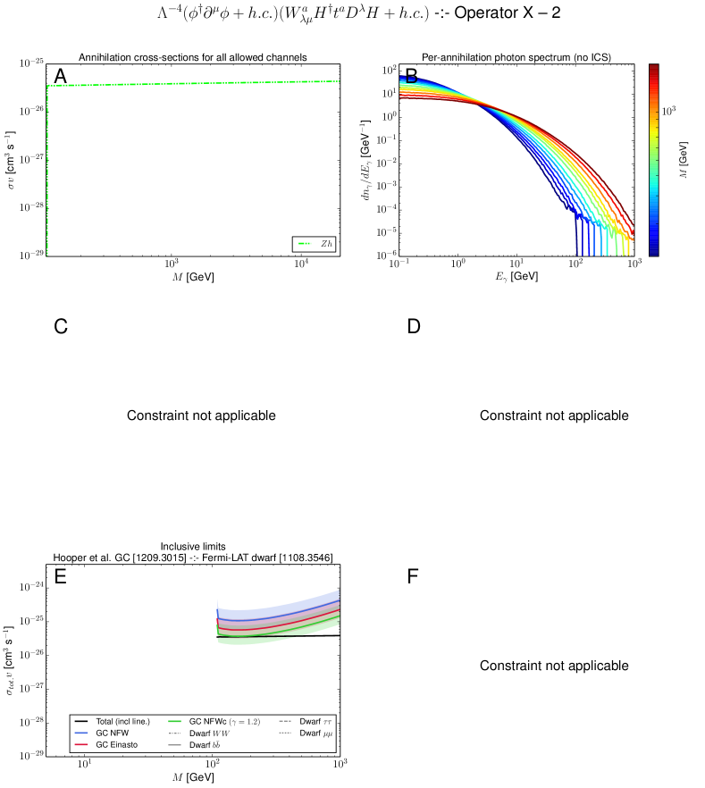
Figure 14: Figure captions are provided in Sec. IV.1 through Sec. IV.6.

These constraints from dwarf galaxies as we have implemented them are conservative and approximate and are not necessarily indicative of the full ability of such measurements to constrain these operators. Based on Fig. 14 of Ref. Hooper et al. (2012), we expect the exclusion reach for an analysis which took into account the entire continuum spectrum at once rather than only looking independently at each component of the spectrum from each final state and comparing to the relevant final state limit from Ref. Ackermann et al. (2011) (thereby paying a cost of BR_f) would be similar to the inclusive galactic center limits from Ref. Hooper et al. (2012) in cases where there are no lines.

Finally, we note that as this paper was being finalized, the Fermi-LAT collaboration released updated constraints stacking 25 dwarf satellites based on 4 years of data Ackermann et al. (2013b). These limits are weaker than expected, and in particular weaker than the limits we take from Ref. Ackermann et al. (2011). However, since these limits are not constraining (as implemented), the updated analysis in Ref. Ackermann et al. (2013b) ultimately does not affect our results.

III.5 Continuum-to-line ratio limits: Cohen et al. analysis

Cohen et al. (2012) finds $5.5\sigma$ (local) evidence for a photon line in the 3.7-year Fermi-LAT data at roughly 130 GeV, and based on the same data, presents limits on the ratio $R$ of the annihilation cross section via modes which give rise to continuum photons, to the annihilation cross section giving lines ($\gamma\gamma$ and/or $\gamma Z$). These limits are based on observations of photon fluxes from Fermi-LAT in the energy range 5 to 200 GeV in an annulus around the GC with inner and outer radii $1^{\circ}$ and $3^{\circ}$, respectively. We compare the two classes of $R$ limits in Ref. Cohen et al. (2012) – shape and supersaturation – to the ratio $R_{\text{th}}=\left(\sigma_{WW}v+\sigma_{ZZ}v+\sigma_{b\bar{b}}v\right)/\left(2\sigma_{\gamma\gamma}v+\sigma_{\gamma Z}v\right)$, computed using the analytical expressions in CKW.

The supersaturation limits on $R$ are derived without assuming a background model, requiring only that the photons from DM annihilation do not supersaturate the observed photon spectrum. These limits are only presented for the case where 100% of the continuum photon flux comes from annihilations going to a $W^{+}W^{-}$ primary final state, but due to the similarity of the spectra, these limits are also applicable if the annihilation is to $ZZ$ or $b\bar{b}$. Although the limits are very conservative, they are more robust to details of astrophysical backgrounds or the DM model than the shape constraints.

We briefly summarize the procedure they followed to obtain the supersaturation limits: for each $M$, the number of line photons was found by performing a maximum likelihood analysis in which the photon lines for $\gamma\gamma$ and $\gamma Z$ were fitted to binned photon-count data, marginalizing over the relative normalization of the lines. The sum of the signal from the two lines was taken as the number of line photons. To find the upper limit on the continuum normalization, the energy bin where the continuum photon spectrum is expected to peak relative to an assumed power-law astrophysical background with a spectral index of 2.8 was first found (this is the only point where spectral information was used); for a pure $WW$ annihilation mode, this was determined to be the bin 10 to 20 GeV. The normalization for the continuum annihilation was then scaled up until the number of photons in the 10 to 20 GeV bin violated the 95% CL UL from data. Correcting for the effective area in Fermi-LAT, this results in a limit on the continuum-to-line cross section ratio.

The second (much stronger) class of limits presented in Ref. Cohen et al. (2012) are shape limits, derived from a maximum likelihood analysis including the two photon lines, the continuum photons, and a single power-law background over the energy range 5 to 200 GeV. At each $M$, the fit was performed for the ratio of continuum-to-line photons in that energy bin, marginalizing over all other parameters including the relative strengths of the two lines. This procedure effectively resulted in a 2-dimensional likelihood profile in the $M-R$ plane; the 2$\sigma$ limit line in this $M-R$ plane is taken as the 95% CL UL on $R$. We consider their results for each of the continuum-photon-producing final states in turn, 100% $WW/ZZ$ and $b\bar{b}$; the $\mu^{+}\mu^{-}$ and $\tau^{+}\tau^{-}$ modes were also considered there, but for our operators annihilation to charged leptons is typically subdominant.

It should be borne in mind that the analysis of Ref. Cohen et al. (2012) marginalized over the $\sigma_{\gamma\gamma}v/\sigma_{\gamma Z}v$ ratio, while the operators here have fixed line ratio for a given $M$. Furthermore, the limits are most applicable if there is some region of $M$ where a good fit to the photon line is possible; note that the line fits are discussed further in Sec. III.7 and also indicated in panel C of our results figures. With more recent data Ackermann et al. (2013a), evidence for the line has weakened, which requires fewer line photons and would lead to correspondingly weaker limits on the continuum-to-line ratio if this analysis were to be updated. Furthermore, Ref. Cohen et al. (2012) assumes 100% annihilation to each of the various continuum-photon-producing modes, while the operators we consider invariably have some combination of multiple continuum-photon-producing annihilation modes. Note also that no inverse Compton scattering (ICS) contribution was included in the continuum spectrum, as it should be sub-dominant for $WW/ZZ$ and $b\bar{b}$, and the contribution to the continuum spectrum of the $Z$ in the $\gamma Z$ channel is not included. Finally, none of the limits presented is applicable to operators with $\gamma h$ final states as this annihilation mode introduces a new line which would dramatically improve the goodness-of-fit in the $M\sim 155$ GeV region.

Nevertheless, even given all these issues, the limits remain indicative for the case where a least one of the annihilation modes $\gamma\gamma$ or $\gamma Z$ is present, and the operator’s continuum photon spectrum is dominated by one of $WW/ZZ$ or $b\bar{b}$. Overall, one should interpret the limits qualitatively, not quantitatively: for operators with continuum-to-photon ratios near the limit, one would really have to be careful in re-doing the full likelihood fit with the correct known branching ratios for the various modes for the specific operator in question to definitively settle the issue of whether or not the operator is excluded.

III.6 Line-like feature: Weniger-like analysis

It is interesting to examine whether it is possible for the photon lines arising from these operators to explain, with the correct normalization, the line-like feature near 130 GeV first reported at $4.6\sigma$ local significance by Weniger (2012) in the 3.7-year Fermi-LAT data, assuming for these purposes that we take this feature seriously as a DM signal.

Assuming the annihilation is to $\gamma\gamma$, Weniger (2012) reports values for $\sigma v$ required to account for this feature. For a $\gamma\gamma$ mode, the DM mass must clearly be 130 GeV to explain the line. For the operators we consider here, there may be annihilation modes to any of the final states $\gamma X$ where $X=\gamma,Z,h$, where the DM mass must be $M=$ 130, 144, and 155 GeV, respectively, to explain the observed line. Eq. (6c) indicates that we must account for this change in mass by performing a rescaling of the cross section result from Ref. Weniger (2012). To be explicit, where an operator has annihilation modes to $\gamma X\ (X=Z,h)$, we rescale the $\gamma\gamma$ result $\left[\sigma v\right]_{\text{Weniger}}$ from Ref. Weniger (2012) as follows:

$$\left[\sigma v\right]_{\gamma X}=2\times 2\times\left(\frac{M}{130\text{ GeV}}\right)^{2}\left[\sigma v\right]_{\text{Weniger}},$$ (20)

where one factor of 2 is due to the assumption of $\gamma\gamma$ and the other factor of 2 is a re-interpretation of a limit set for self-conjugate DM in Weniger (2012) to our choice of fermion or complex scalar DM [see Eq. (6c)]. In addition, we perform the rescaling necessary to account for differing halo profile normalizations, as discussed in Sec. II.3.1; the rescaling factors we use are given in Table 2.

Owing once again to the only partial resolution in the Fermi-LAT data of the photon lines, we cannot naïvely use the required line cross section from Ref. Weniger (2012) to give individual required cross sections for the $\gamma\gamma$ and $\gamma Z$ modes when both are present (see discussion in Sec. III.1). Assuming either $M=130$ GeV or $M=144$ GeV, the secondary line at either 114 or 144 GeV, respectively, would give a significant photon contribution at the position of the line at 130 GeV and/or vice versa depending on the relative normalizations of the lines. Similarly, since the line separation here is still on the order of the Fermi-LAT energy resolution (even if assumed to be 10%), one also cannot assume the lines are completely unresolved to derive a single required combined value for $(2\sigma_{\gamma\gamma}+\sigma_{\gamma Z})v$.

Nevertheless, while we acknowledge this issue, for the purpose of giving a rough estimate of the annihilation cross section which would be required for our operators with both $\gamma\gamma$ and $\gamma Z$ annihilation modes to explain the line reported at 130 GeV in Ref. Weniger (2012), we have performed the following approximate analysis. We note that it is usually the case that one or other of the lines from either the $\gamma\gamma$ or $\gamma Z$ mode is dominant for $M$ in the approximate range 120 to 150 GeV (in terms of photon flux, for operators VI-1, IV-2, VIII-1, or VIII-2, it is the $\gamma\gamma$ mode which dominates by about a factor of 4, while for operators VI-3, VI-4, VIII-3, or VIII-4, it is the $\gamma Z$ mode which dominates by about a factor of 2.5). Therefore, we shall make the approximation that the line at 130 GeV reported in Ref. Weniger (2012) is entirely due to the dominant of the $\gamma X\ (X=\gamma,Z)$ modes. As noted above, there will be a second line in either case, but we ignore this complication in our approximate treatment here (see the next section for a slightly more careful treatment of the same issue making use of results from a different reference). We give results for the quantity $\left(2\sigma_{\gamma\gamma}+\sigma_{\gamma Z}\right)v$, requiring that the normalization of the dominant mode can explain the line at 130 GeV. To be explicit, if the $\gamma X\ (X=\gamma,Z)$ annihilation mode explains the line at 130 GeV, we extend Eq. (20) above to the two-line case:

$$\left[\left(2\sigma_{\gamma\gamma}+\sigma_{\gamma Z}\right)v\right]=2\times 2\times\left(\dfrac{M}{130\text{ GeV}}\right)^{2}\left[\sigma v\right]_{\text{Weniger}}\times\left\{\begin{array}[]{ll}\left[1+\dfrac{\sigma_{\gamma Z}v(M)}{2\sigma_{\gamma\gamma}v(M)}\right]&\text{for }M=130\ \text{GeV, }\ X=\gamma\\[17.22217pt] \left[1+\dfrac{2\sigma_{\gamma\gamma}v(M)}{\sigma_{\gamma Z}v(M)}\right]&\text{for }M=144\ \text{GeV, }X=Z\end{array}\right..$$ (23)

The factors in the brackets $[\ \cdots\ ]$ are computed using the analytical expressions in CKW and merely rescale the individual required $\sigma_{\gamma X}v\ (X=\gamma,Z)$ cross sections for the line at 130 GeV to the quantity $\left(2\sigma_{\gamma\gamma}+\sigma_{\gamma Z}\right)v$.

III.7 Line-like features: Cohen et al. analysis

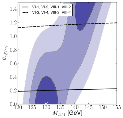
Figure 3: Contours adapted from Fig. 2 in Cohen et al. (2012). The colored bands shown here in order of decreasing darkness are the $1$-, $2$-, and $3$-$\sigma$ delta-log-likelihood contours for the line-existence analysis performed in Cohen et al. (2012), in which $\gamma\gamma$ and $\gamma Z$ lines plus a power-law background were fitted to the 3.7-year Fermi-LAT data; the white cross at $M=130$ GeV and $\theta_{\gamma Z/\gamma\gamma}=\arctan\left(N_{\gamma Z}/N_{\gamma\gamma}\right)=0$ is the best fit point corresponding to a $5.5\sigma$ local significance relative to a null hypothesis of no line. The solid and dashed black lines are the theoretical results for the relative normalization of the two lines $\theta_{\gamma Z/\gamma\gamma}=\arctan\left(\sigma_{\gamma Z}v/2\sigma_{\gamma\gamma}v\right)$, as computed using the analytical cross section formulae in CKW for the eight operators which have both lines present. Although there are eight operators, the results fall onto only two curves, which are indicated on the figure. There is clearly a region of $M$ parameter space for any of these operators where the relative line normalization is such that the double-line provides a good (delta-log-liklihood $<1\sigma$) fit to the Fermi-LAT data.

In addition to presenting limits for the ratio of continuum-to-line cross sections, Cohen et al. (2012) also presents evidence for the existence for a line in the Fermi-LAT 3.7-year data in an annulus centered on the GC with inner and outer radii of $1^{\circ}$ and $3^{\circ}$, respectively, with local significance of 5.5$\sigma$ relative to the null hypothesis of no line. To reach this conclusion, they performed a likelihood analysis fitting binned photon count data in the energy range 5 to 200 GeV to a single power-law background plus lines at $E_{\gamma}=M$ (with normalization $N_{\gamma\gamma}$) and at $E_{\gamma}=M-m_{Z}^{2}/4M$ (with normalization $N_{\gamma Z}$), both suitably convolved with the Fermi-LAT energy dispersion. No continuum photon contribution from DM annihilation was included in this analysis. In the fit, $M$ and $\theta_{\gamma Z/\gamma\gamma}=\arctan\left(N_{\gamma Z}/N_{\gamma\gamma}\right)$ were scanned over while the background normalization and spectral index, as well as the total line normalization $N_{\gamma\gamma}+N_{\gamma Z}$, were marginalized over. The best fit point for this analysis was found to be $M=130$ GeV and $\theta_{\gamma Z/\gamma\gamma}=0$. (An earlier analysis Rajaraman et al. (2012) fitting the data with $\gamma\gamma$ and $\gamma Z$ lines found very similar results; we have followed Cohen et al. (2012) since that work also gave limits on the continuum-to-line ratio.)

Cohen et al. (2012) presents $1$-, $2$-, and $3$-$\sigma$ delta-log-likelihood contours for their fitting procedure in the $M-\theta_{\gamma Z/\gamma\gamma}$ plane, which we have reproduced in Fig. 3, along with the theoretical values for $\theta_{\gamma Z/\gamma\gamma}=\arctan\left(\sigma_{\gamma Z}v/2\sigma_{\gamma\gamma}v\right)$ for the eight operators that have both $\gamma\gamma$ and $\gamma Z$ lines, as computed using the analytical expressions of CKW. We see that the relative normalizations of the lines for these operators are such there are regions around $M=130$ GeV or $M=144$ GeV where the sum of the two lines could fit the Fermi-LAT data very well (within $1\sigma$ in delta-log-likelihood).

Cohen et al. also gives contours displaying the total normalization (photon count) $N_{\text{total}}\equiv N_{\gamma\gamma}+N_{\gamma Z}$ of the lines in the $M-\theta_{\gamma Z/\gamma\gamma}$ plane which, knowing the ROI-averaged mission-time-integrated exposure-times-effective-area $\mathcal{E}_{\text{ROI}}$ relevant to the Fermi-LAT data they considered, would allow us to extract the cross sections required for the operators with both $\gamma\gamma$ and $\gamma Z$ modes to explain the fitted lines. As $\mathcal{E}_{\text{ROI}}$ was not relevant to the analysis presented in Ref. Cohen et al. (2012), it was not given there. However, we have made use of the Fermi ScienceTools package to reproduce a sufficient portion of the data-extraction and analysis in that reference to enable us to compute it ourselves (see Appendix C for the full details of our analysis and the cross-checks we have performed). We find that the ROI-averaged exposure factor for photon energies from ca. 120 to 150 GeV (applicable to the line-fits presented in Ref. Cohen et al. (2012)) is $\mathcal{E}_{\text{ROI}}=1.05\times 10^{11}$cm²s. Knowing this factor, and extracting the fitted total line-normalization $N_{\text{total}}$ from the contours in Fig. 2 of Cohen et al. (2012), we have computed the photon flux corresponding to the fitted line normalization as

$$\Phi=\frac{N_{\text{total}}}{\mathcal{E}_{\text{ROI}}}.$$ (24)

Finally, making use of Eq. (6c) we have converted this to the annihilation cross section required as a function of $M$ to explain the line for our particular operators having both $\gamma\gamma$ and $\gamma Z$ modes,

$$(2\sigma_{\gamma\gamma}+\sigma_{\gamma Z})v=\frac{16\pi M^{2}}{J}\Phi=\frac{16\pi M^{2}}{J}\frac{N_{\text{total}}}{\mathcal{E}_{\text{ROI}}},$$ (25)

for the (operator-specific) range of $M$ within the 3$\sigma$ $|$delta-log-likelihood$|$ contours shown in Fig. 3. In performing this conversion, we have also computed the $J$ factors for the ROI in Ref. Cohen et al. (2012), which we give in Appendix C.

IV Results

In Figs. 4 through 37 we present the indirect detection limits for all operators with $s$-wave annihilations as studied in CKW. The cross sections for various operators are listed in Tables VI-XX of CKW. We refer to a process studied in CKW by a table number, and an operator number. For instance, operator VI-3 is the third operator of Table VI in CKW, in this case, $\phi^{\dagger}\phi W^{a}_{\ \mu\nu}W^{a\,\mu\nu}$. Our notation for field operators will follow the notation in CKW.

There is one figure for each operator consisting of up to six panels. The captions for each panel are the same for each figure and described below. In addition, we make operator-specific comments in some individual figure captions.

IV.1 Panel A:

We show the non-relativistic DM annihilation cross sections $\sigma v$ as a function of DM mass for each of the annihilation modes allowed for the particular EFT operator, assuming that a) the DM annihilates only through that operator and b) the DM particle is a thermal relic with $\Omega_{DM}h^{2}=0.12$.

If all annihilation modes are pure $s-$wave, the total cross section for annihilation attains a value of around $\sigma v\approx 3.6\times 10^{-26}$cm³s^-1 for $M=100$ GeV [showing logarithmic variation with $M$; cf. Eq. (1)]. However, $p-$wave components to some annihilation channels can cause the the present-day total annihilation cross section to be suppressed due to their non-negligible impact in the early universe when the relic density is set; these contributions naturally drive $\Lambda$ larger and hence the present-day annihilation cross section smaller. This effect is particularly pronounced in operators where the $s-$wave annihilation is essentially independent of $M$ but the $p-$wave annihilation contribution grows with $M$, e.g., the operator XVII-1, $\Lambda^{-4}\bar{\chi}\gamma^{\mu 5}\chi i\left(B_{\lambda\mu}Y_{H}H^{\dagger}D^{\lambda}H-\text{h.c.}\right)$.

Ignoring kinematic thresholds, for all final states involving fermions except those in Table IX of CKW, the fermion contributions separate into four distinct types: leptons with $T^{3}=\pm 1/2$ and quarks with $T^{3}=\pm 1/2$ (cf., the results for all operators XVIII-XX).

IV.2 Panel B:

The per-annihilation total differential spectrum $dN_{\gamma}/dE_{\gamma}=\sum_{f}\text{BR}_{f}\cdot dN^{f}_{\gamma}/dE_{\gamma}$ of prompt gamma rays as a function of $E_{\gamma}$ is plotted for different values of DM mass, indicated by the color scale. The mass dependence of the spectra depends on whether the dominant final states are fermions or if they are gauge bosons and Higgs. In the latter case, the spectrum becomes harder with increasing DM mass because the final states become more boosted. Further details on these spectra can be found in Sec. II.4. No inverse Compton scattering (ICS) component is included. An estimate of the error introduced by neglect of ICS is given in Appendix A.

IV.3 Panel C:

If applicable, this panel shows the line search limits for the DM mass region 5 GeV to approximately 300 GeV from the Fermi-LAT Ackermann et al. (2013a) line search using observed photon fluxes from the Galactic center. We show these limits in terms of the total annihilation rate to monochromatic photons (i.e., the annihilation rate to each final state weighted by the number of monochromatic photons in that final state). The solid black line shows the specific $\sigma v$ required for a thermal relic.

The solid colored lines show 95% CL UL for various halo profiles and ROIs, assuming the central values for halo normalization $\rho_{\odot}$ from Ref. Iocco et al. (2011) (see Table 1). The like-colored bands show the variation in the UL as $\rho_{\odot}$ is varied through $2\sigma$ limits. For operators with multiple possible lines (i.e., $\gamma\gamma$ and $\gamma Z$ annihilation modes) we do not set limits in the region of DM masses 80 GeV to 160 GeV where we expect the Fermi-LAT line shape would become a very broad or double-peaked structure (see Sec. III.1).

If present, the colored squares with their error bars represent $(M,\sigma v)$ values where the operator in question could additionally supply the line reported in Weniger (2012), assuming the central values for $\rho_{\odot}$ for each halo profile. As discussed in Sec. III.6, for operators where there are multiple photon lines we make the assumption that the line at 130 GeV is due to the dominant photon line mode.

For operators with $\gamma\gamma$ and $\gamma Z$ lines, we show colored lines near 130-150 GeV, which indicate the cross sections required to explain a possible double-line feature in the Fermi-LAT data based on the analysis of Cohen et al. (2012) as extended by us in Appendix C. The opacity of the colored band around each line indicates the delta-log-likelihood of the double-line fit compared to the best-fit point, with the darkest band being $1\sigma$, the medium band being $2\sigma$ and the lightest being $3\sigma$. The central line corresponds to the central value of the halo profile normalization, with the shaded band vertically giving the $\pm 2\sigma$ normalization uncertainties on the halo profiles.

IV.4 Panel D:

If applicable, this panel shows the line search limits for the WIMP mass region from 500 GeV to 20 TeV from the H.E.S.S Abramowski et al. (2013) line search discussed in Sec. III.2. The ROI is a circle of radius $1^{\circ}$ centered on the GC with Galactic latitudes $|b|<0.3^{\circ}$ excluded. Note the change from Panel C to a logarithmic scale in $M$.

The black and solid colored lines and similarly colored bands are all as described in Panel C. Isothermal limits are very weak for this line search owing to the cored nature of the profile and very small ROI near the GC.

IV.5 Panel E:

This panel shows the inclusive (continuum and line) spectrum limits for DM mass from 5 GeV to 1 TeV based on the “model-independent” limits given in Hooper et al. (2012) and described in Sec. III.3. These are given as the solid colored lines labelled ‘GC …’; the colored bands show the range of halo profile normalizations, as in Panel C. The solid black line is the result for the total $\sigma v$ for the operator.

The sharp features in the GC limits that can be seen in some cases are due to the $\gamma$ lines changing through the bins used in Hooper et al. (2012). For operators with lines only from $\gamma Z$ or $\gamma h$, we also see sharp features in the limits near threshold as the line energy migrates rapidly across the bins; had we convolved the lines with the Fermi-LAT energy dispersion, these cross-over regions would be smoothed.

Also shown are Fermi-LAT Ackermann et al. (2011) stacked dwarf galaxy limits, discussed in Sec. III.4. These are given as a variety of grey lines and are a conservative estimate of the 95% CL UL limits; because the published limits were presented in terms of specific final states, there is not enough information to fully derive the limits for the continuum spectra here.

IV.6 Panel F:

If applicable, the limits presented here are on the ratio of selected continuum final state annihilation cross sections to the line final states $\gamma\gamma$ and $\gamma Z$ as described in Cohen et al. (2012) and summarized in Sec. III.5; these limits are only applicable if the operator has no final state $\gamma h$, and has dominant annihilation branching ratios to at least one of the final states $WW/ZZ$ or $b\bar{b}$.

The solid black line is the ratio $R_{\text{th}}\equiv\left(\sigma_{WW}v+\sigma_{ZZ}v+\sigma_{b\bar{b}}v\right)/\left(2\sigma{\gamma\gamma}v+\sigma_{\gamma Z}v\right)$ for this operator; the dashed colored lines are individual annihilation mode contributions to this summed result. The various solid colored lines give either the supersaturation 95% CL UL on $R$ for fixed $M$, or the boundary of the ‘$2\sigma$’ confidence region in the $R-M$ plane for the shape constraints from Cohen et al. (2012) assuming 100% annihilation to the indicated final state. Further discussion of the applicability of these limits is given in the text in Sec. III.5, but it should be borne in mind that operators which are only marginally excluded or allowed per the results given here merit further investigation to determine whether or not they are actually excluded. In particular, the continuum radiation from the $Z$ in $\gamma Z$ is not factored in. Furthermore, the ratio of $\gamma\gamma$ to $\gamma Z$ is not fixed at the correct ratio for each operator here considered, but is rather marginalized over in the analysis of Ref. Cohen et al. (2012).

V Discussion and Conclusions

Table 3: Classification of operators by limit results. Starred (*) categories have operators which could fit the Fermi 130 GeV $\gamma$-ray line and also match the correct relic abundance.

#	Labels	Operators	Summary of annihilation modes and limits
1	VI-1	$\phi^{\dagger}\phi\ B_{\mu\nu}B^{\mu\nu}$	$\gamma\gamma$ is present and dominant for all masses, leading to strong line limits for masses up to 10 TeV; $\gamma Z$ and $ZZ$ enter above kinematic thresholds but are sequentially more parametrically suppressed by powers of $(\sin\theta_{W}/\cos\theta_{W})^{2}$.
	VI-2	$\phi^{\dagger}\phi\ \widetilde{B}_{\mu\nu}B^{\mu\nu}$
	VIII-1	$\bar{\chi}i\gamma^{5}\chi\ B_{\mu\nu}B^{\mu\nu}$
	VIII-2	$\bar{\chi}i\gamma^{5}\chi\ \widetilde{B}_{\mu\nu}B^{\mu\nu}$
2	XI-1	$\left(\phi^{\dagger}\partial^{\mu}\phi+\text{h.c.}\right)i\left(B_{\lambda\mu}Y_{H}H^{\dagger}D^{\lambda}H-\text{h.c.}\right)$	$\gamma X$ and $ZX$ where $X=Z$ (for “$-\text{h.c.}$” operators) OR $X=h$ (for “$+\text{h.c.}$”) are present above thresholds, with the latter in each case typically suppressed by $(\sin\theta_{W}/\cos\theta_{W})^{2}$. Line limits are constraining up to a TeV.
	XI-2	$\left(\phi^{\dagger}\partial^{\mu}\phi+\text{h.c.}\right)i\left(\widetilde{B}_{\lambda\mu}Y_{H}H^{\dagger}D^{\lambda}H-\text{h.c.}\right)$
	XIV-1	$\bar{\chi}\gamma^{\mu}\chi\left(B_{\lambda\mu}Y_{H}H^{\dagger}D^{\lambda}H+\text{h.c.}\right)$
	XIV-2	$\bar{\chi}\gamma^{\mu}\chi\left(\widetilde{B}_{\lambda\mu}Y_{H}H^{\dagger}D^{\lambda}H+\text{h.c.}\right)$
	XV-1	$\bar{\chi}\gamma^{\mu}\chi i\left(B_{\lambda\mu}Y_{H}H^{\dagger}D^{\lambda}H-\text{h.c.}\right)$
	XV-2	$\bar{\chi}\gamma^{\mu}\chi i\left(\widetilde{B}_{\lambda\mu}Y_{H}H^{\dagger}D^{\lambda}H-\text{h.c.}\right)$
3	XVII-1	$\bar{\chi}\gamma^{\mu 5}\chi\ i\left(B_{\lambda\mu}Y_{H}H^{\dagger}D^{\lambda}H-\text{h.c.}\right)$	$\gamma Z$ and $ZZ$ are present above thresholds. Line limits are constraining up to a few hundred GeV, however $p$-wave components to the annihilation cross section during the freeze out become important at larger DM mass leading to suppression of the $s$-wave component and significant weakening of constraints.
	XVII-2	$\bar{\chi}\gamma^{\mu 5}\chi\ i\left(\widetilde{B}_{\lambda\mu}Y_{H}H^{\dagger}D^{\lambda}H-\text{h.c.}\right)$
4	XVIII-1	$\bar{\chi}\gamma^{\mu\nu}\chi\ B_{\mu\nu}Y_{H}H^{\dagger}H$	Annihilation to fermions is dominant and $s$-wave at low WIMP mass, with strong inclusive limits. The $\gamma h$ line annihilation mode becomes dominant above threshold, and the line limits are constraining for masses of 100 GeV up to a few TeV.
5	XVIII-2	$\bar{\chi}\gamma^{\mu\nu}\chi\ \widetilde{B}_{\mu\nu}Y_{H}H^{\dagger}H$	Similar to the operator above, but the continuum final states are $p$-wave, so inclusive limits not constraining below 70 GeV.
6*	VI-3	$\phi^{\dagger}\phi\ W^{a}_{\mu\nu}W^{a\ \mu\nu}$	$\gamma\gamma$ is present for all masses; $\gamma Z$, $ZZ$ and $WW$ enter above kinematic thresholds. Above the $W^{+}W^{-}$ threshold, annihilation modes with lines are heavily parametrically suppressed by powers of $\sin^{2}\theta_{W}$. Line searches are constraining below the $W^{+}W^{-}$ threshold.
	VI-4	$\phi^{\dagger}\phi\ \widetilde{W}^{a}_{\mu\nu}W^{a\ \mu\nu}$
	VIII-3	$\bar{\chi}i\gamma^{5}\chi\ W^{a}_{\mu\nu}W^{a\ \mu\nu}$
	VIII-4	$\bar{\chi}i\gamma^{5}\chi\ \widetilde{W}^{a}_{\mu\nu}W^{a\ \mu\nu}$
7*	XI-3	$\left(\phi^{\dagger}\partial^{\mu}\phi+\text{h.c.}\right)i\left(W_{\lambda\mu}H^{\dagger}t^{a}D^{\lambda}H-\text{h.c.}\right)$	$\gamma X$, $ZX$ and $W^{+}W^{-}$ where $X=Z\ (``-\text{h.c.}")\text{ OR }h\ (``+\text{h.c.}")$ are present above thresholds. Line limits are severely constraining for masses less than around 100 GeV; once the $W^{+}W^{-}$ mode enters, the $\gamma X$ annihilation mode is heavily suppressed. Inclusive limits are weakly constraining for masses up to a few hundred GeV. Where applicable, the ratio limits are either marginal or quite constraining on 125-150 GeV.
	XI-4	$\left(\phi^{\dagger}\partial^{\mu}\phi+\text{h.c.}\right)i\left(\widetilde{W}^{a}_{\lambda\mu}H^{\dagger}t^{a}D^{\lambda}H-\text{h.c.}\right)$
	XIV-3	$\bar{\chi}\gamma^{\mu}\chi\left(W^{a}_{\lambda\mu}H^{\dagger}t^{a}D^{\lambda}H+\text{h.c.}\right)$
	XIV-4	$\bar{\chi}\gamma^{\mu}\chi\left(\widetilde{W}^{a}_{\lambda\mu}H^{\dagger}t^{a}D^{\lambda}H+\text{h.c.}\right)$
	XV-3	$\bar{\chi}\gamma^{\mu}\chi i\left(W^{a}_{\lambda\mu}H^{\dagger}t^{a}D^{\lambda}H-\text{h.c.}\right)$
	XV-4	$\bar{\chi}\gamma^{\mu}\chi i\left(\widetilde{W}^{a}_{\lambda\mu}H^{\dagger}t^{a}D^{\lambda}H-\text{h.c.}\right)$
8*	XVII-3	$\bar{\chi}\gamma^{\mu 5}\chi\ i\left(W^{a}_{\lambda\mu}H^{\dagger}t^{a}D^{\lambda}H-\text{h.c.}\right)$	Similar to the category just above, but $p$-wave components to the cross section cause suppression of the $s$-wave cross section and weaken line constraints above a few hundred GeV.
	XVII-4	$\bar{\chi}\gamma^{\mu 5}\chi\ i\left(\widetilde{W}^{a}_{\lambda\mu}H^{\dagger}t^{a}D^{\lambda}H-\text{h.c.}\right)$
9	XIX-1	$\bar{\chi}\gamma^{\mu\nu}\chi\ W^{a}_{\mu\nu}H^{\dagger}t^{a}H$	Annihilation to continuum modes is dominant, and inclusive limits are constraining up to a hundred GeV.
10	XIX-2	$\bar{\chi}\gamma^{\mu\nu}\chi\ \widetilde{W}^{a}_{\mu\nu}H^{\dagger}t^{a}H$	Annihilation to continuum modes dominates, but are $p$-wave at low DM masses.
11	IX-2	$\bar{\chi}i\gamma^{5}\chi\ H^{\dagger}H$	Only continuum annihilation modes exist: one of either the $f\bar{f}$ or $W^{+}W^{-}$ modes dominate at all masses.
	XX-1	$\bar{\chi}\gamma^{\mu\nu}\chi\ B_{\mu\nu}$
12	X-1	$\left(\phi^{\dagger}\partial^{\mu}\phi+\text{h.c.}\right)\left(B_{\lambda\mu}Y_{H}H^{\dagger}D^{\lambda}H+\text{h.c.}\right)$	Only $Zh$ $s$-wave modes are present.
	X-2	$\left(\phi^{\dagger}\partial^{\mu}\phi+\text{h.c.}\right)\left(W^{a}_{\lambda\mu}H^{\dagger}t^{a}D^{\lambda}H+\text{h.c.}\right)$
13	XVI-1	$\bar{\chi}\gamma^{\mu 5}\chi\ \left(B_{\lambda\mu}Y_{H}H^{\dagger}D^{\lambda}H+\text{h.c.}\right)$	Only $Zh$ $s$-wave modes are present but there are also significant $p$-wave contributions.
	XVI-3	$\bar{\chi}\gamma^{\mu 5}\chi\ \left(W^{a}_{\lambda\mu}H^{\dagger}t^{a}D^{\lambda}H+\text{h.c.}\right)$

Broadly speaking, we find that the 34 operators with $s$-wave annihilation channels can be classified into thirteen qualitatively distinct classes on the basis of the limits which apply to each operator; we summarize these in Table 3.

• Operators coupling to hypercharge gauge bosons; photon lines present (categories 1-3)

  For operators in the first 3 categories in Table 3, annihilation to final states giving lines has a large branching fraction as soon as the dark matter mass is larger than lowest kinematical threshold for such channels. This is a consequence of the fact that the $B$ field strength tensor has a dominant photon component so that couplings to the $Z$ are parametrically suppressed with respect to couplings to the $\gamma$ by a factor of $\tan^{2}\theta_{W}\sim 0.3$ (this suppression may be partially invalidated by other large factors arising in the evaluation of the matrix element, but nevertheless serves as a useful rule-of-thumb). As a result, the operators in categories 1 and 2 are excluded at 95% confidence by the Fermi-LAT Ackermann et al. (2013a) and H.E.S.S. Abramowski et al. (2013) line limits for most masses from the lowest kinematic threshold for a line final state up to a few TeV, except a) if the very conservative isothermal profile choice is made for the H.E.S.S. limits and b) the dark-matter mass is in the region 300 GeV and 500 GeV, which is not addressed by any of the line limits. Depending on the profile choice, the required thermal cross section for these operators may also be in tension with the experimental upper limits from a few to 20 TeV.

  For operators in category 3, the total $s$-wave cross section drops away from the canonical thermal value of approximately $3\times 10^{-26}$cm³s^-1 as $M^{-2}$ for $M$ above a few hundred GeV. This phenomenon occurs generically for operators with fermion DM coupling via an axial-vector $J_{DM}$ current, and is due to the presence of $p$-wave components to the annihilation cross section which are enhanced over the $s$-wave by a factor of $s/m_{V}^{2}\sim M^{2}$. This enhancement can be traced to a coupling in the $p$-wave (but not the $s$-wave) to the longitudinal component $\epsilon^{\mu}_{L}\sim k^{\mu}/m_{Z}$ of the massive vector. Since both $s$- and $p$-wave components of $\sigma v$ can be important at freeze-out [cf. Eq. (1)], having $a/b\sim M^{-2}$ naturally suppresses the present-day annihilation cross section for large $M$ by driving up the value of $\Lambda$ required to saturate the present-day average DM density. As a result, a significantly smaller range of $M$ is definitively excluded by, or put in tension with, the experimental limits compared to categories 1 and 2, especially for TeV-range DM. The constraints from the inclusive limits from Ref. Hooper et al. (2012) are less stringent: in most cases, the limits are in tension with the thermal relic cross section for $M$ below one or two hundred GeV only for some choices of halo profile, except for operators with $\gamma\gamma$ modes where, below ca. 100 GeV, the inclusive limits exclude such operators even for conservative profile choices.

• Operators coupling to $SU(2)_{L}$ gauge bosons and Higgs; photon lines present (categories 6-8)

  For operators coupling to the $SU(2)_{L}$ gauge bosons and Higgs (entries 6–8 in Table 3), the $W^{+}W^{-}$ final state is always dominant for $M\gtrsim m_{W}$ since in this case couplings to the $Z$ and $\gamma$ are parametrically suppressed by $\cos^{2}\theta_{W}$ and $\sin^{2}\theta_{W}$, respectively. Consequently, for operators in categories 6 and 7, the line limits are only severely constraining between the lowest kinematic threshold for any line mode and $M\simeq m_{W}$; for $M$ greater than about $100$ GeV and less than a few TeV the experimental limits are typically either only in tension with the required thermal cross section for more aggressive choices of halo profile, or are completely unconstraining. Operators in category 8 again contain fermion DM with coupling via an axial-vector current and thus suffer the same falling $\sigma v$ at large $M$ as the operators in category 3, and as a result are even less constrained at large $M$ than the operators in categories 6 and 7. The inclusive limits from Ref. Hooper et al. (2012) are somewhat stronger for all these operators than for the operators in categories 1–3, and may be in tension with the required thermal cross section up to a few hundred GeV depending on the profile choice. Nevertheless, taken together with the line limits, these operators are only weakly constrained for heavy DM.

  In addition, for most operators in categories 6–8, the shape-based ratio limits Cohen et al. (2012) are either very constraining (operators XI-3 and XVII-3), or are marginal in the sense that the current limit is very close to the predicted value from the operators. We however caution the reader that the limits in Ref. Cohen et al. (2012) were obtained by assuming the line signal would account for the Fermi signal for some choice of DM mass, and allowing the relative strengths of the lines to float to the optimal value. The first assumption may or may not be applicable to our analysis depending on the operator considered; but the second is never applicable to our analysis since the relative strengths of all annihilation channels are fixed for any given operator. Therefore, marginal cases may or may not actually be constrained by these limits and a more careful analysis is needed here.

• Operators with annihilation modes to fermions; photon lines present (categories 4,5,9,10)

  The analysis in Ref. Hooper et al. (2012) as applied to our operators indicates that if the only available $s$-wave annihilation mode for $M<10$ GeV dark matter is to Standard Model fermions, there is a strong constraint which seems to rule out the annihilation cross section necessary for obtaining the thermal relic abundance for $M<10$ GeV.

  The operators listed in entries 4, 5, 9 and 10 of Table 3 all have annihilation modes to both fermions and line final states (amongst others). Of these, the operators coupling to the field-strength tensor (rather than its dual) have $s$-wave annihilation to $f\bar{f}$ final states and so can be excluded for $M$ below 10 GeV; they may also be in tension with the inclusive limits, depending on the profile choice, from 10 GeV to a few hundred GeV. Also, for these operators, the branching ratio to $f\bar{f}$ annihilation modes falls once the on-shell diboson modes become kinematically allowed. This is because the annihilation to fermions goes through $s$-channel gauge boson exchange and so requires an additional Higgs vev insertion and coupling of fermions to $\gamma/Z$ compared to the $Zh$ and $\gamma h$ modes (see the next paragraph for a comment on the $W^{+}W^{-}$ mode). On dimensional grounds this results in a suppression of the $f\bar{f}$ modes relative to the $Zh$ and $\gamma h$ modes by a factor $\sim m_{Z,W}^{2}/s$ (where $s\sim 4M^{2}$). For the operators coupling instead to the dual field strength tensor, the fermion cross section is $p$-wave so the inclusive limits are less constraining: they may be in tension with the required cross section from the $\gamma h$ threshold to a few hundred GeV, but only for fairly aggressive profile choices.

  For the operators in categories 4 and 5 with couplings to hypercharge and Higgs, the photon line becomes strong above the kinematic threshold for the $\gamma h$ annihilation mode leading to strongly excluding line constraints, whereas for the operators in categories 8 and 9 with couplings to the $SU(2)_{L}$ gauge bosons and Higgs, the diboson annihilation modes are dominated by $W^{+}W^{-}$, which leads to line limits for these operators in tension with the required thermal cross section only if an aggressive profile choice is made. We note that this occurs notwithstanding the fact that for the $W^{+}W^{-}$ mode (as for the $f\bar{f}$ mode), both Higgs fields must be replaced by their vevs; the reason that this does not suppress this final state is that there is a cancellation of the suppression factor $\sim m_{W}^{2}/s$ against an enhancement $\sim s/m_{W}^{2}$ from the longitudinal mode of the $W^{\pm}$ (the by-now-familiar suppression, relative to $W^{\pm}$, of couplings to $Z$ and $\gamma$ by weak-mixing-angle factors accounts for the relative strength of the $W^{+}W^{-}$ and $Zh$ or $\gamma h$ modes).

• Operators without photon lines (categories 11-13)

  Finally, entries 11–13 in Table 3 are operators which couple only to SM final states without photon lines. The two operators in entry 11 have strong annihilation to $f\bar{f}$ either for all $M$ (operator XX-1) or at low $M$ (operator IX-2), but in either case this means that they are strongly constrained for $M\lesssim 10$ GeV even for conservative profile choices. Owing to the very flat (with changing $M$) nature of the inclusive upper limits on $\sigma v$, the astrophysical uncertainty gives a rather broad range of $M$ for which the operators may be in tension with the experimental limits depending on the profile choice: 10 GeV to a few hundred GeV. The operators in entries 12 and 13 have only $Zh$ final states: the former may be in tension with the astrophysical limits for aggressive profile choices for $M$ between 100 and 400 GeV, but they are unconstrained for more modest profile choices; the latter are unconstrained regardless of the profile chosen due to $s$-wave cross section suppression by the same enhanced–$p$-wave effect which was discussed at length above.

In addition to these indirect limits, we emphasize the point made in CKW that the ‘tensor’ fermion DM currents $\chi\gamma^{\mu\nu}\chi$ (e.g., operators XVIII-n, XIX-n and XX-n in categories 4-5 and 9-11) give rise to magnetic or electric dipole couplings (if necessary, by replacing both Higgs fields with their vevs) which causes them to be very strongly constrained by direct detection experiments Banks et al. (2010); Fortin and Tait (2011). Given our assumptions about the DM being a cold thermal relic WIMP saturating the measured average density, the operators giving electric-dipole couplings (coupling to the dual field tensor) are excluded at at least 90% confidence by both CDMS and XENON across the entire mass range from $M=10$ GeV to at least 20 TeV (probably somewhat larger), while the operators giving magnetic-dipole couplings (coupling to the field tensor, not its dual) are excluded at at least 90% confidence from $M=10$ GeV to $M>20$ TeV, $M\simeq 1$ TeV, or $M\simeq 400$ GeV for operators XX-1, XVIII-1, or XIX-1, respectively (with the exception of a very narrow mass window around $m_{Z}/2$ for the latter two of these).

We have presented all of our results under the assumption that fermionic DM is Dirac, however the compensating factors of 2 in Eqs. (1) and (6c) imply that there is a uniform shifting of all $\sigma v$ values down by a factor of 2 if Majorana fermion DM was assumed instead; therefore, the same thermal cross section relative to all of our 95% CL UL limits would obtain, at least for all the operators which do not vanish identically for Majorana fermion DM.

$\gamma$-ray Line Signals

As discussed in Sec. III.6 and Sec. III.7, there is some evidence, first reported by Weniger (2012), for a photon line in the Fermi-LAT data near 130 GeV (updated to approximately 133 GeV in Ref. Ackermann et al. (2013a)) with a flux matching DM annihilation into monochromatic photons with cross section $\sigma v\approx 10^{-27}$ cm³/s. Although the most recent official Fermi-LAT collaboration analysis Ackermann et al. (2013a) finds less significant evidence for this putative line-like feature, it cannot fully explain it as a systematic effect, and cautions that more work is needed to understand it. If we however take this signal seriously, we find that there are a number of operators (indicated in Table 3 by a superscript star) which could plausibly explain it which are not yet excluded by either the upper limits on the continuum emission or by the latest official Fermi-LAT limits on lines.

The signal strength for the photon line is a factor of a few (up to an order of magnitude, depending on the halo profile) below the thermal relic cross section. Operators with annihilation into $SU(2)_{L}$ gauge bosons (categories 6–8) naturally give a suppression of this size simply from the mixing angle $\sin^{2}\theta_{W}$. Numerical factors are also important, and those operators with smaller branching ratios into lines do not produce enough monochromatic photons if the cross section is fixed by the matching onto the correct relic density. To put it another way, these operators may be in some tension with continuum limits or the constraint on the continuum-to-line ratio since the BR to such continuum modes is then larger.

Operators XV-3 and XV-4 are most promising as explanation of the line, but for completeness we also note that almost any of the other operators in categories 6–8 in Table 3 could also work, including VI-3, VI-4, VIII-3, VIII-4, XI-4, XIV-3, XIV-4, and XVII-4. The operators XI-3 and XVII-3 have smaller branching ratios to lines, less than 10$\%$, and so do not fit the line as well for the reasons discussed above. However, given the systematic uncertainties, it is not yet conclusive that these operators cannot explain the Fermi gamma-ray line. (Finally, although the operators XVIII-1 and XIX-2 also have lines of roughly the correct strength, they are ruled out by direct detection experiments, as discussed above.)

Other Indirect Constraints and Outlook

Photon fluxes do not of course supply the only prospects for indirect detection of dark matter. At present, the IceCube experiment Aartsen et al. (2013); Abbasi et al. (2012) reports limits on $\sigma v$ from neutrino fluxes which are at best on the order of $10^{-22}-10^{-23}$cm³s^-1, which are thus much too weak to be constraining. The absence of sharp spectral features in the AMS-02 positron fraction data provides a constraint Bergstrom et al. (2013) on annihilation modes giving a sharp edge in the positron fraction: we expect that these limits could be stronger than the GC inclusive limits for $M$ less than a few tens of GeV for operators with sizeable BR for annihilation to $e^{+}e^{-}$, and to a lesser extent $\mu^{+}\mu^{-}$, final states (operators XVIII-1, XIX-1, IX-2 and XX-1; the latter may be more constrained since $f\bar{f}$ dominates for all masses). A slightly different analysis Kopp (2013) constraining only the total number of positrons from various DM annihilation modes using a combination of Fermi-LAT and AMS-02 data confirms the approximate equivalence of the limits from positron measurements and the GC inclusive photon flux limits for the $\mu^{+}\mu^{-}$ annihilation mode, but indicates that constraints arising from positron measurements for other channels ($b\bar{b},\ W^{+}W^{-},\ ZZ$) would be between one and two orders of magnitude weaker than the GC inclusive photon flux limits. Additionally, constraints from antiproton fluxes may be useful to consider. Ref. Cotta et al. (2012) found that the PAMELA antiproton limits are typically weaker than the inclusive GC photon flux limits for $W^{+}W^{-}$ or $b\bar{b}$ annihilation modes and do not typically have sufficient reach to exclude the thermal WIMP scenario for at least some of the operators we have considered; however, Ref. Cirelli and Giesen (2013) finds that antiproton bounds are roughly comparable with the GC inclusive photon limits from Ref. Hooper et al. (2012) for pure $b\bar{b}/t\bar{t}$ or $W^{+}W^{-}/ZZ$ final states for $M\gtrsim 100$ GeV (the antiproton limits are much weaker for smaller $M$ or for leptonic annihilation modes), but which have fairly large uncertainties arising from cosmic ray propagation models. One would have to fully reconstruct the analysis of Ref. Cirelli and Giesen (2013) to take advantage of these comparable limits though, since independently comparing the individual mode cross sections to their respective limits would again be subject to the cost of a factor of BR_f, which is usually fairly small for $b\bar{b}$ or $t\bar{t}$ modes for our operators.

Looking forward, Ref. Bergström et al. (2012) indicates that it would be appropriate to consider a factor of 3-5 improvement in the present best limits from the next generation of indirect detection experiments looking at photon fluxes (GAMMA-400, CTA, H.E.S.S.-II). This magnitude of improvement would be able to constrain a fair amount more of the parameter space for the mass of the thermal relic WIMP scenario even factoring in the astrophysical uncertainties, but would still not be able to completely rule out all DM masses for every EFT operator with $s$-wave annihilation channels which we have considered.

Figure 4: Figure captions are provided in Sec. IV.1 through Sec. IV.6.

Figure 5: Figure captions are provided in Sec. IV.1 through Sec. IV.6.

Figure 6: Figure captions are provided in Sec. IV.1 through Sec. IV.6. This operator may be compatible with present experimental limits and capable of accounting for the 130 GeV photon line for some profile choices.

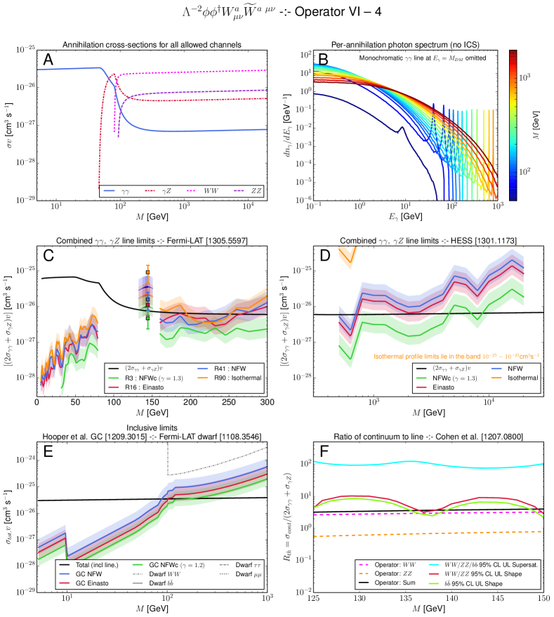
Figure 7: Figure captions are provided in Sec. IV.1 through Sec. IV.6.This operator may be compatible with present experimental limits and capable of accounting for the 130 GeV photon line for some profile choices.

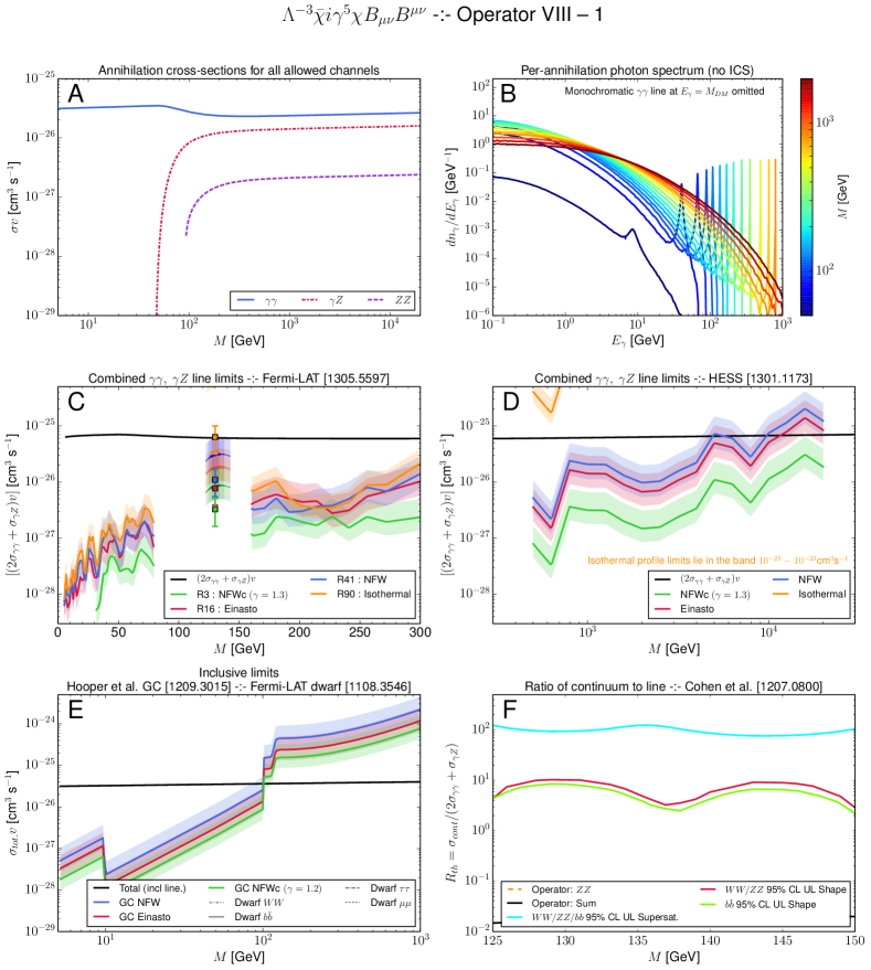
Figure 8: Figure captions are provided in Sec. IV.1 through Sec. IV.6.

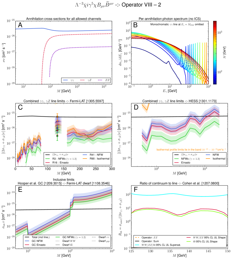
Figure 9: Figure captions are provided in Sec. IV.1 through Sec. IV.6.

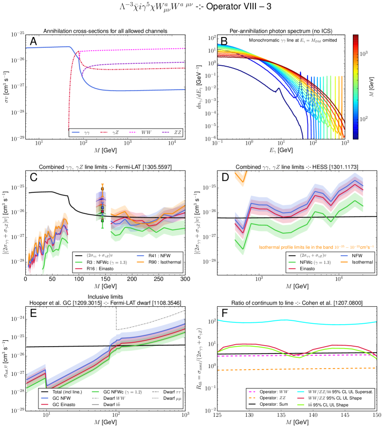
Figure 10: Figure captions are provided in Sec. IV.1 through Sec. IV.6. This operator may be compatible with present experimental limits and capable of accounting for the 130 GeV photon line for some profile choices.

Figure 11: Figure captions are provided in Sec. IV.1 through Sec. IV.6. This operator may be compatible with present experimental limits and capable of accounting for the 130 GeV photon line for some profile choices.

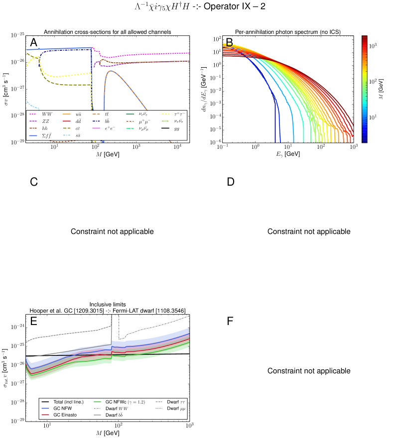
Figure 12: Figure captions are provided in Sec. IV.1 through Sec. IV.6. The DM annihilation for this operator proceeds via $s$-channel Higgs exchange (except for the $4$-body contact contribution to the $hh$ final state), and we have only utilized the cross sections for the 2-body on-shell final states that couple at tree-level to the $h$; we have however checked that including the loop-induced couplings to the $gg$ final state makes only a negligible difference to the limits. We have not quantitatively estimated the effect of the $3$- or $4$-body branchings involving intermediate off-shell $W/Z$ bosons, but again we would not expect the limits to change too dramatically.

Figure 13: Figure captions are provided in Sec. IV.1 through Sec. IV.6.

Figure 15: Figure captions are provided in Sec. IV.1 through Sec. IV.6.

Figure 16: Figure captions are provided in Sec. IV.1 through Sec. IV.6.

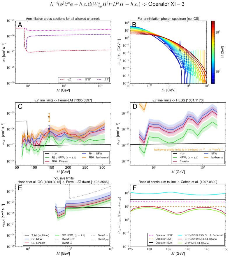
Figure 17: Figure captions are provided in Sec. IV.1 through Sec. IV.6. This operator may be compatible with present experimental limits and capable of accounting for the 130 GeV photon line for some profile choices, although the line BR is somewhat small.

Figure 18: Figure captions are provided in Sec. IV.1 through Sec. IV.6. This operator may be compatible with present experimental limits and capable of accounting for the 130 GeV photon line for some profile choices.

Figure 19: Figure captions are provided in Sec. IV.1 through Sec. IV.6.

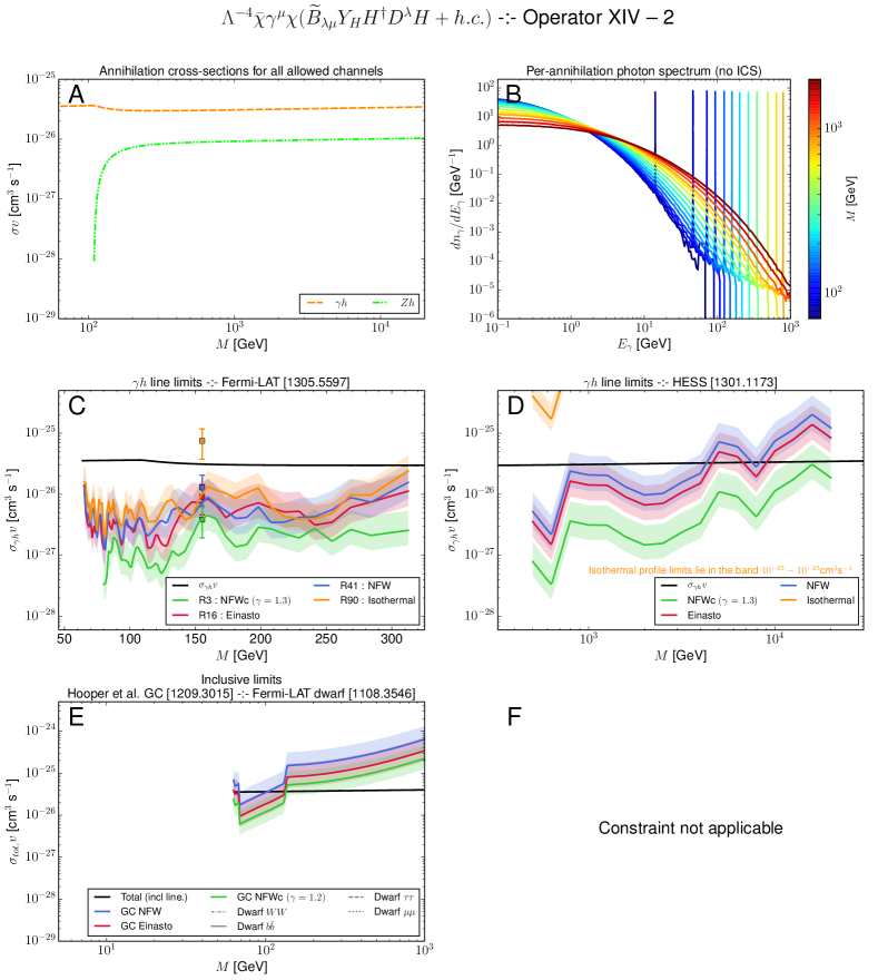
Figure 20: Figure captions are provided in Sec. IV.1 through Sec. IV.6.

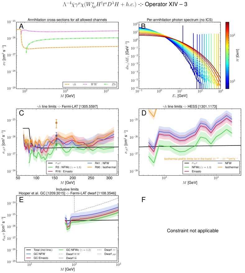
Figure 21: Figure captions are provided in Sec. IV.1 through Sec. IV.6. This operator may be compatible with present experimental limits and capable of accounting for the 130 GeV photon line for some profile choices.

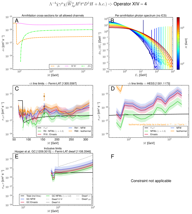
Figure 22: Figure captions are provided in Sec. IV.1 through Sec. IV.6. This operator may be compatible with present experimental limits and capable of accounting for the 130 GeV photon line for some profile choices.

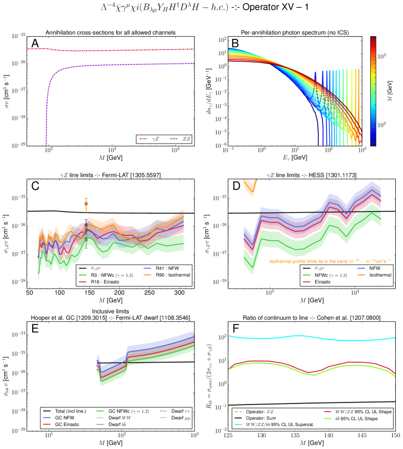
Figure 23: Figure captions are provided in Sec. IV.1 through Sec. IV.6.

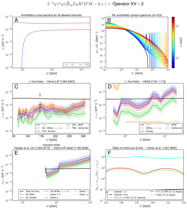
Figure 24: Figure captions are provided in Sec. IV.1 through Sec. IV.6.

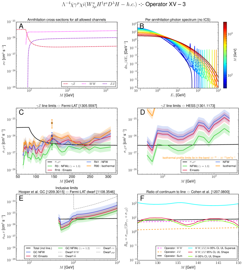
Figure 25: Figure captions are provided in Sec. IV.1 through Sec. IV.6. This operator may be compatible with present experimental limits and account well for the 130 GeV photon line for some profile choices.

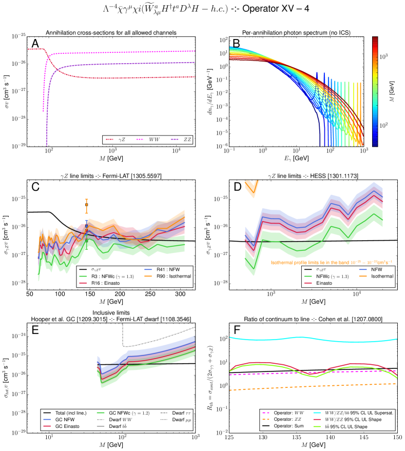
Figure 26: Figure captions are provided in Sec. IV.1 through Sec. IV.6. This operator may be compatible with present experimental limits and account well for the 130 GeV photon line for some profile choices.

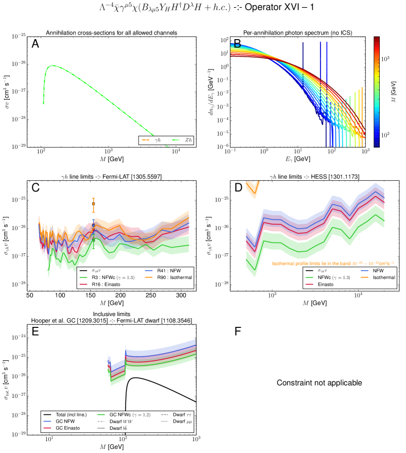
Figure 27: Figure captions are provided in Sec. IV.1 through Sec. IV.6. The $\gamma h$ mode is $p$-wave suppressed and so $\sigma_{\gamma h}v$ is orders of magnitude below the range of cross sections shown in panels C and D.

Figure 28: Figure captions are provided in Sec. IV.1 through Sec. IV.6. The $\gamma h$ mode is $p$-wave suppressed and so $\sigma_{\gamma h}v$ is orders of magnitude below the range of cross sections shown in panels C and D.

Figure 29: Figure captions are provided in Sec. IV.1 through Sec. IV.6.

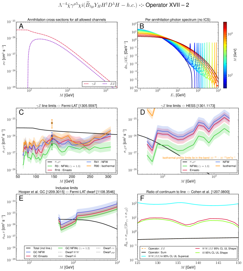
Figure 30: Figure captions are provided in Sec. IV.1 through Sec. IV.6.

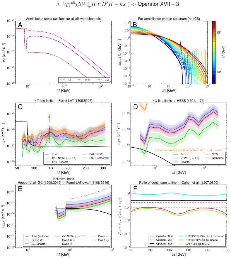
Figure 31: Figure captions are provided in Sec. IV.1 through Sec. IV.6. This operator may be compatible with present experimental limits and capable of accounting for the 130 GeV photon line for some profile choices, although the line BR is somewhat small.

Figure 32: Figure captions are provided in Sec. IV.1 through Sec. IV.6. This operator may be compatible with present experimental limits and capable of accounting for the 130 GeV photon line for some profile choices.

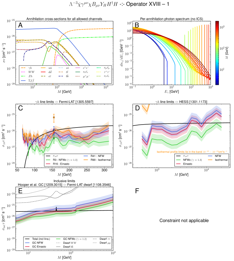
Figure 33: Figure captions are provided in Sec. IV.1 through Sec. IV.6. This operator may be compatible with present experimental limits and account well for the 130 GeV photon line for some profile choices; however, this operator gives rise to a magnetic dipole coupling of the DM and as such is excluded at 90% confidence by the CDMS and XENON direct detection experiments Banks et al. (2010); Fortin and Tait (2011) for $M$ from 10 GeV to ca. 1 TeV.

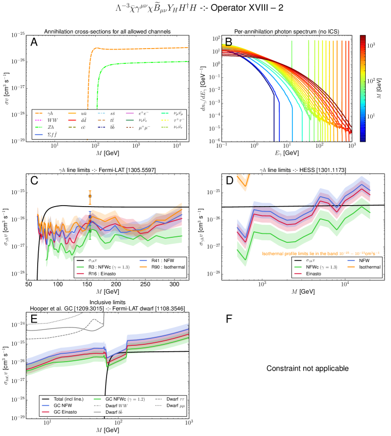
Figure 34: Figure captions are provided in Sec. IV.1 through Sec. IV.6. This operator gives rise to an electric dipole coupling of the DM and as such is excluded at 90% confidence by the CDMS and XENON direct detection experiments Banks et al. (2010); Fortin and Tait (2011) for the entire range of $M$ shown here.

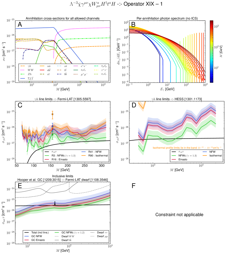
Figure 35: Figure captions are provided in Sec. IV.1 through Sec. IV.6. This operator gives rise to a magnetic dipole coupling of the DM and as such is excluded at 90% confidence by the CDMS and XENON direct detection experiments Banks et al. (2010); Fortin and Tait (2011) for $M$ from 10GeV to ca. 400GeV.

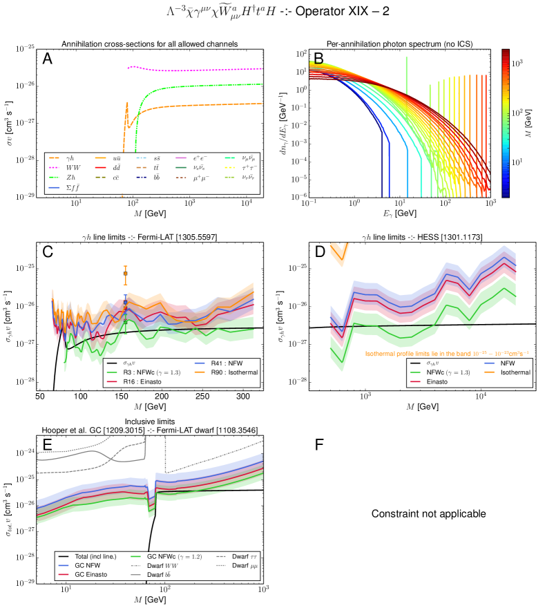
Figure 36: Figure captions are provided in Sec. IV.1 through Sec. IV.6. This operator may be compatible with present experimental limits and capable of accounting for the 130 GeV photon line for some profile choices; however, this operator gives rise to an electric dipole coupling of the DM and as such is excluded at 90% confidence by the CDMS and XENON direct detection experiments Banks et al. (2010); Fortin and Tait (2011) for the entire range of $M$ shown here.

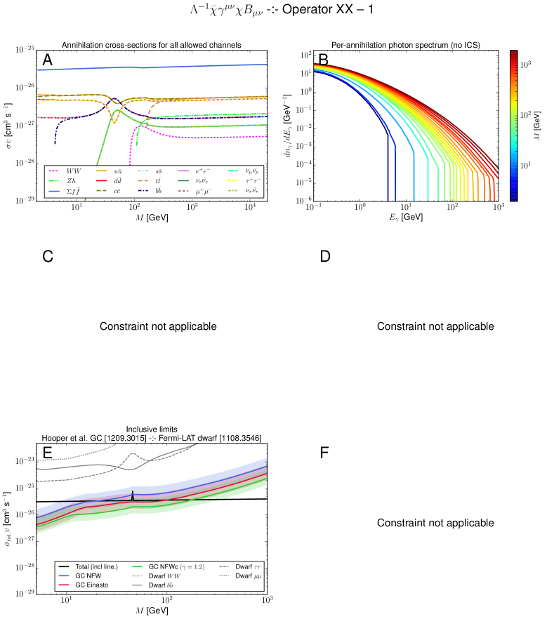
Figure 37: Figure captions are provided in Sec. IV.1 through Sec. IV.6. This operator gives rise to a magnetic dipole coupling of the DM and as such is excluded at 90% confidence by the CDMS and XENON direct detection experiments Banks et al. (2010); Fortin and Tait (2011) for the entire range of $M$ shown here.

Appendix A Inverse Compton Scattering

In addition to prompt photons, there may be gamma rays resulting from Inverse Compton Scattering (ICS) of any electrons/positrons injected into the GC radiation field. ICS is most relevant for annihilation modes which inject energy primarily in the form of $e^{\pm}$, in particular the $e^{+}e^{-}$ or $\mu^{+}\mu^{-}$ modes. For the heavy quark or diboson primary final states relevant for most of the operators, the effect of ICS at high energies is subdominant compared to the prompt gamma rays produced by pion decay. Although the ICS contribution can dominate at lower photon energies, the most constraining limits for continuum emission typically come from the 10-100 GeV energy range, so we do not expect significant changes to results for these operators.

There are some operators which have direct annihilation to charged fermions. However, even for these operators the charged lepton annihilation modes are relevant only for masses below the thresholds for diboson final states, and here the inclusive limits are already constraining. For example, in the case of operator IX-2 Fig. 16, the fermion contributions are proportional to $m_{f}^{2}$, so only the $\tau^{+}\tau^{-}$ annihilation mode is relevant, and only for $M\lesssim 100$ GeV. For all other operators where fermion final states are present the charged leptons typically comprise no more than 40% of the total charged fermion branching fraction, and only are relevant below a few hundred GeV (with the exception of Operator XX-1, Fig. 37). We thus do not expect a very large correction to the limits we have set when the ICS photons are included.

Here we demonstrate that including ICS will not change limits significantly by giving a quantitative estimate for operators with charged fermion final states. We will make use of the results of Cirelli et al. (2010), which give pre-computed Green functions $I_{\text{IC}}(E_{s},E_{\gamma},l,b)$ that allow one to convert from an electron injection spectrum to an ICS photon spectrum, taking into account the various $e^{\pm}$ energy-loss mechanisms in the GC.

It is important to note that the morphologies of the prompt and ICS photon signals will not in general be exactly the same, since the ICS signal depends on the galactic radiation fields as well as the energy loss and diffusion of the injected electrons. As detailed in Sec. III.3, our primary source of inclusive spectrum limits is Hooper et al. (2012) and the limits in that reference are extracted for $E_{\gamma}\in[0.1,100]$ GeV from the upper limit of the normalization of a prompt-photon signal template $\propto\int_{\text{LOS}}\rho^{2}(r[s,l,b])ds$ smoothed over $0.5^{\circ}$ regions. The limits set in that analysis are therefore not applicable for photon signal components which do not follow approximately the same morphology as prompt photons. That said, we find morphological differences give rise to only a factor of a few variation in the ratio of the ICS to prompt signal when considered over $\mathcal{O}(10^{\circ})$ regions. We therefore take the approximation of the limits in Ref. Hooper et al. (2012) being applicable to the combined ICS and prompt photon signals.

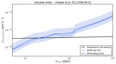
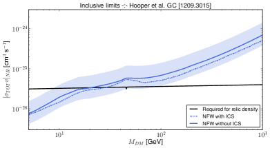
Figure 38: An example of the impact on the inclusive limits when ICS is included (subject to the approximations discussed in the text). These results are for operators XVIII-1 (left panel) and XX-1 (right panel) and are representative of the most dramatic effect seen for any operator: even so, the effect on the limits is well within the astrophysical uncertainties.

Since we are not however reproducing the template subtraction analysis, we must make a choice for the ROI over which to extract the effective ICS spectrum in order to make a direct comparison with the cross section limits in Ref. Hooper et al. (2012). Motivated by the cuspy nature of the expected signal morphologies, and the fact that the photon signal used in setting the limits in that reference is mostly contained within a region of about $3^{\circ}$ around the GC, we chose to utilize a $5^{\circ}$ radius circular region centered on the GC in extracting the effective ICS spectra. Furthermore, at very high injection energies, the high-energy ICS signal is more constrained to the galactic center, since electrons must be at high energy to create high energy photons via single Klein-Nishina-regime Compton scatters, and this only happens near the point of production as the electrons lose energy as they propagate out of the GC region.

We integrate the ICS signal over this ROI and normalize by the line of sight integral for that region:

$$\left.\frac{dN^{\text{ICS}}_{\gamma}}{dE_{\gamma}}\right|_{\text{ROI}} =\frac{1}{E_{\gamma}^{2}}\times\left[\int_{m_{e}}^{M}\!\!\!\!\!dE_{s}\ \left(\sum_{f}\text{Br}_{f}\frac{dN^{f\text{, inj. }}_{e^{\pm}}}{dE_{s}}\right)\ \int_{\text{ROI}}d\Omega\ I_{\text{IC}}(E_{s},E_{\gamma},l,b)\right]\times\left[\int_{\text{LOS-ROI}}d\Omega\frac{ds}{r_{\odot}}\left(\frac{\rho\left(r\right)}{\rho_{\odot}}\right)^{2}\right]^{-1}.$$ (26)

This gives an effective ROI-averaged per-annihilation spectrum of up-scattered ICS photons, in terms of the constituent electron injection spectra $dN^{f\text{, inj.}}_{e^{\pm}}/dE_{s}$, for final state $f$, and where $E_{s}\in[m_{e},M]$ is the energy of the injected electron, $E_{\gamma}$ is the energy on the up-scattered ICS photon and $l,b,s,r$ are coordinates and distances as defined in the main text A fairly conservative estimate for the systematic uncertainty here is $\pm 50$% due to the choice of ROI. Note finally that the diffusion setups MIN, MED, MAX (discussed in Cirelli et al. (2010)) give largely similar results for an ROI of this size near the GC.

Explicitly checking the shift in the limits set using the results of Hooper et al., we find that the limits are strengthened by no more than a factor of 1.4 at any $M$ for any operator, which is well within the astrophysical uncertainty due to the normalization of the halo profile. The resulting effect on the limit is shown for a representative case in Fig. 38.

Appendix B Estimate of systematic uncertainties

It is useful to have an approximate knowledge of the size of various systematic uncertainties which impact our results and which we have not explicitly included in the main body of the paper. We summarize the systematics in Table 4. It is relatively clear that the astrophysical (halo profile normalization) uncertainties dominate the systematics, but depending on the result and mass range in question, it may be prudent to take the total systematic uncertainty as something up to twice as large as the astrophysical uncertainty.

Table 4: Estimated maximum systematic uncertainties from various effects, quoted as the percentage variation in the $\sigma v$ limit: $f\equiv 100\times\left(\left[\sigma v\right]^{\text{95\% CL UL}}_{\text{effect accounted for}}-\left[\sigma v\right]^{\text{95\% CL UL}}_{\text{limit as presently set}}\right)/\left[\sigma v\right]^{\text{95\% CL UL}}$ (so $f<0$ means a more stringent limit with the effect properly accounted for, while $f>0$ means the limit as currently set is too stringent). Values estimated by us are marked with a ^⋆; values taken from the relevant literature source are not marked. For comparison, the typical variation between the most conservative normalization for the most conservative profile choice and the most aggressive normalization for the cuspiest profile is about an order of magnitude, so relative to the mid-point the astrophysical uncertainties can cause the limit to vary by about $+100\%$ / $-75\%$.

Result(s) affected	Description of effect	Variation in result $f$
All	Halo rescaling or $J$ factor computation	$\pm 5\%^{\star}$
Ackermann et al. (2013a) line limits	Variations in the fitted signal strength due to the finite spacing between tested values of the scanned line peak energy and estimate of the energy resolution	$+12\%$ / $-7\%$
Ackermann et al. (2013a) line limits	Variations in the effective exposure used in converting the fitted number of photons in a line to a flux	$\pm 16\%$
Ackermann et al. (2013a) line limits	Fake or masked signals: for low WIMP masses (a few tens of GeV), up to roughly the size of the statistical uncertainties, which are about a factor of 2.	$+100\%$ / $-50\%$ for low masses, dropping rapidly as mass increases
Ackermann et al. (2013a) line limits	Correctly accounting for the $\gamma Z$ photon linewidth	$+7\%$
Ackermann et al. (2013a) line limits	Mis-modelling of the photon line shape for the cases with both $\gamma\gamma$ and $\gamma Z$ peaks in the vicinity of $M\sim 80$GeV and $M\sim 160$ GeV.	$+10\%^{\star}$
Abramowski et al. (2013) line limits	Overall systematics estimate	$+50\%$ / $-50\%$
Hooper et al. (2012) inclusive limits	Subtraction of additional background associated with Galactic Ridge or central gamma-ray point source	$-50\%$
Hooper et al. (2012) inclusive limits	Uncertainty in the exact value of the “fudge-factor” of 2.8 necessary to resolve the discrepancy noted in the main body	$\pm 10\%^{\star}$
Hooper et al. (2012) inclusive limits	Including ICS photons in setting the limit (estimated using the $5^{\circ}$ ROI normalization; the systematic uncertainty on the normalization of ICS spectrum itself is about $\pm 50\%$ owing to our approximate treatment)	$-40\%^{\star}$
Ackermann et al. (2011) continuum limits	Excluding from the limit computation the two most uncertain spherical dwarf measurements	$+50\%$
Weniger (2012) line fit	Overall systematics estimate	$+15\%$ / $-20\%$

Table 5: The $J$ factors for the $1^{\circ}-3^{\circ}$ annular ROI defined in Cohen et al. (2012). Unless otherwise indicated, these results assume the central normalization and parameter values from Table 1.

Halo Profile	$J$ factor [1021 GeV2 cm-5]
NFWc ($\gamma=1.3$)	$32.50$
Einasto	$15.05$
NFW	$9.02$
Isothermal	$0.361$
Einasto with $R_{\odot}=8.5$ kpc and $\rho_{\odot}=0.4$ GeV/cm3	$21.41$

Appendix C Exposure for line fit in annular region

In Sec. III.7 we describe the application of the line-fit results of Cohen et al. (2012) to operators with both $\gamma\gamma$ and $\gamma Z$ lines. However, Cohen, et al. supplied only fitted values of $N_{\gamma\gamma}+N_{\gamma Z}$. In order to apply their results, a necessary ingredient is the exposure: the mission-time integrated effective observing area multiplied by the observing time, averaged over the ROI. In this Appendix we summarize our calculation of the exposure for their reported data set.

We have reproduced their data-extraction using the Fermi ScienceTools v9r31p1 software with the publicly available Fermi-LAT weekly data files. To be explicit, we have considered data on the time interval 239557447—356400002 (in Mission Elasped Time), with photon energy range 5-200 GeV in an annular region centered on the GC with inner and outer radii of $1^{\circ}$ and $3^{\circ}$ respectively. We use the P7_V6_ULTRACLEAN data set and filter the data using option 2 as recommended for a diffuse analysis. Histogramming the photon counts in the annular ROI we reproduce almost exactly the counts presented in Tables II and III of Ref. Cohen et al. (2012).

We compute the full-sky exposure map as a function of photon energies near $125-150$ GeV, and subselect the annular ROI from the full-sky exposure map (exposure values in angular bins). The ROI-averaged exposure is given by

$$\mathcal{E}_{\text{ROI}}=\frac{1}{\Delta\Omega}\int_{\Delta\Omega}\mathcal{E}(\Omega)d\Omega\approx\frac{1}{\Delta\Omega}\sum_{i}\mathcal{E}_{i}\cos b_{i}\Delta l\Delta b,$$ (27)

where $\Delta\Omega=7.65\times 10^{-3}$sr, $\mathcal{E}_{i}$ is the exposure value in angular bin $i$, and the sum runs over all angular bins (which have angular size $\Delta l\times\Delta b=0.1^{\circ}\times 0.1^{\circ}$). Strictly speaking, one should weight the exposure by the signal morphology before performing the integration in Eq. (27); however, the very small size of the ROI together with the almost uniform exposure over the ROI make neglecting this subtlety a good approximation. We find that the exposure does not vary significantly over the energy range $125-150$ GeV, and takes a value of $\mathcal{E}_{\text{ROI}}=1.05\times 10^{11}$cm²s.

The photon flux corresponding to the line is given by $({N_{\gamma\gamma}+N_{\gamma Z}})/{\mathcal{E}_{\text{ROI}}}$. We find the total normalization $N_{\gamma\gamma}+N_{\gamma Z}$ for each operator using a 2D polynomial interpolation of the contour map given in Fig. 2 of Ref. Cohen et al. (2012), extracting the value of $N_{\gamma\gamma}+N_{\gamma Z}$ on the operator-specific curves indicated in Fig. 3. Finally, we compute the $J$ factors necessary to extract cross sections from these fluxes given the central normalization values in Table 1; the results are in Table 5. Applying Eq. (25), we thus interpret the fit results in terms of the annihilation cross section to lines, $(2\sigma_{\gamma\gamma}+\sigma_{\gamma Z})v$; we plot this quantity in our result plots on the regions of $M$ parameter space where the delta-log-likelihood for the double line fit is $\leq 3\sigma$, $\leq 2\sigma$ and $\leq 1\sigma$ (see Fig. 3).

To check our work, we compare with the analysis of a single line presented in Ref. Weniger (2012). We compute the value of $\sigma_{\gamma\gamma}v=(8\pi M^{2}/2J)N_{\gamma\gamma}/\mathcal{E}_{\text{ROI}}$ assuming $\theta_{\gamma z/\gamma\gamma}=0$, $N_{\gamma\gamma}=33$ and $M=130$ GeV, along with the Einasto profile $J$ factor at the bottom of Table 5 which has been computed using the indicated parameter values taken from Ref. Weniger (2012). We obtain $\sigma_{\gamma\gamma}v=3.2\times 10^{-27}$cm³s^-1, which is a factor of 3 larger than the central value ($\sigma_{\gamma\gamma}v=1.1\times 10^{-27}$cm³s^-1) reported in Ref. Weniger (2012). There is thus some tension between these two analyses.

References

- Ade et al. (2013) P. A. R. Ade et al. (Planck Collaboration), (2013), arXiv:1303.5076 [astro-ph.CO] .
- Beltran et al. (2009) M. Beltran, D. Hooper, E. W. Kolb, and Z. C. Krusberg, Phys.Rev. D80, 043509 (2009), arXiv:0808.3384 [hep-ph] .
- Beltran et al. (2010) M. Beltran, D. Hooper, E. W. Kolb, Z. A. Krusberg, and T. M. Tait, JHEP 1009, 037 (2010), arXiv:1002.4137 [hep-ph] .
- Goodman et al. (2011) J. Goodman, M. Ibe, A. Rajaraman, W. Shepherd, T. M. Tait, et al., Phys.Lett. B695, 185 (2011), arXiv:1005.1286 [hep-ph] .
- Goodman et al. (2010) J. Goodman et al., Phys. Rev. D82, 116010 (2010), arXiv:1008.1783 [hep-ph] .
- Fox et al. (2012a) P. J. Fox, R. Harnik, J. Kopp, and Y. Tsai, Phys.Rev. D85, 056011 (2012a), arXiv:1109.4398 [hep-ph] .
- Fox et al. (2012b) P. J. Fox, R. Harnik, R. Primulando, and C.-T. Yu, Phys.Rev. D86, 015010 (2012b), arXiv:1203.1662 [hep-ph] .
- Rajaraman et al. (2011) A. Rajaraman, W. Shepherd, T. M. Tait, and A. M. Wijangco, Phys.Rev. D84, 095013 (2011), arXiv:1108.1196 [hep-ph] .
- Fox et al. (2011) P. J. Fox, R. Harnik, J. Kopp, and Y. Tsai, (2011), arXiv:1103.0240 [hep-ph] .
- Aad et al. (2012) G. Aad et al. (ATLAS Collaboration), (2012), arXiv:1210.4491 [hep-ex] .
- ATL (2012) Search for New Phenomena in Monojet plus Missing Transverse Momentum Final States using 10fb-1 of pp Collisions at sqrts=8 TeV with the ATLAS detector at the LHC, Tech. Rep. ATLAS-CONF-2012-147 (CERN, Geneva, 2012).
- Chatrchyan et al. (2012) S. Chatrchyan et al. (CMS Collaboration), JHEP 1209, 094 (2012), arXiv:1206.5663 [hep-ex] .
- CMS (2013) Search for new physics in monojet events in pp collisions at sqrt(s)= 8 TeV, Tech. Rep. CMS-PAS-EXO-12-048 (CERN, Geneva, 2013).
- Lin et al. (2013) T. Lin, E. W. Kolb, and L.-T. Wang, (2013), arXiv:1303.6638 [hep-ph] .
- Chen et al. (2013) J.-Y. Chen, E. W. Kolb, and L.-T. Wang (CKW), (2013), arXiv:1305.0021 [hep-ph] .
- Ackermann et al. (2013a) M. Ackermann et al. (Fermi-LAT Collaboration), (2013a), arXiv:1305.5597 [astro-ph.HE] .
- Abramowski et al. (2013) A. Abramowski et al. (H.E.S.S. Collaboration), (2013), arXiv:1301.1173 [astro-ph.HE] .
- Hooper et al. (2012) D. Hooper, C. Kelso, and F. S. Queiroz, (2012), arXiv:1209.3015 [astro-ph.HE] .
- Ackermann et al. (2011) M. Ackermann et al. (Fermi-LAT Collaboration), (2011), arXiv:1108.3546 [astro-ph.HE] .
- Weniger (2012) C. Weniger, (2012), arXiv:1204.2797 [hep-ph] .
- Cohen et al. (2012) T. Cohen, M. Lisanti, T. R. Slatyer, and J. G. Wacker, (2012), arXiv:1207.0800 [hep-ph] .
- Cotta et al. (2012) R. Cotta, J. Hewett, M. Le, and T. Rizzo, (2012), arXiv:1210.0525 [hep-ph] .
- Weiner and Yavin (2012) N. Weiner and I. Yavin, Phys.Rev. D86, 075021 (2012), arXiv:1206.2910 [hep-ph] .
- Weiner and Yavin (2013) N. Weiner and I. Yavin, Phys.Rev. D87, 023523 (2013), arXiv:1209.1093 [hep-ph] .
- Rajaraman et al. (2013) A. Rajaraman, T. M. Tait, and A. M. Wijangco, Phys.Dark Univ. 2, 17 (2013), arXiv:1211.7061 [hep-ph] .
- Rajaraman et al. (2012) A. Rajaraman, T. M. Tait, and D. Whiteson, JCAP 1209, 003 (2012), arXiv:1205.4723 [hep-ph] .
- Shoemaker and Vecchi (2012) I. M. Shoemaker and L. Vecchi, Phys.Rev. D86, 015023 (2012), arXiv:1112.5457 [hep-ph] .
- Busoni et al. (2013) G. Busoni, A. De Simone, E. Morgante, and A. Riotto, (2013), arXiv:1307.2253 [hep-ph] .
- Buchmueller et al. (2013) O. Buchmueller, M. J. Dolan, and C. McCabe, (2013), arXiv:1308.6799 [hep-ph] .
- Kolb and Turner (1994) E. W. Kolb and M. S. Turner, The Early Universe (Westview Press, 1994).
- Iocco et al. (2011) F. Iocco, M. Pato, G. Bertone, and P. Jetzer, (2011), arXiv:1107.5810 [astro-ph.GA] .
- Ackermann et al. (2012a) M. Ackermann et al. (Fermi-LAT Collaboration), (2012a), arXiv:1205.2739 [astro-ph.HE] .
- Catena and Ullio (2009) R. Catena and P. Ullio, (2009), arXiv:0907.0018 [astro-ph.CO] .
- (34) O. Y. Gnedin, A. V. Kravtsov, A. A. Klypin, and D. Nagai, astro-ph/0406247 .
- Barger et al. (2012) V. Barger, M. Ishida, and W.-Y. Keung, (2012), arXiv:1203.3456 [hep-ph] .
- Sjöstrand et al. (2007) T. Sjöstrand, S. Mrenna, and P. Skands, (2007), arXiv:0710.3820 [hep-ph] .
- Cirelli et al. (2010) M. Cirelli, G. Corcella, A. Hektor, G. Hütsi, M. Kadastik, P. Panci, M. Raidal, F. Sala, and A. Strumia, (2010), arXiv:1012.4515 [hep-ph] .
- Ciafaloni et al. (2010) P. Ciafaloni, D. Comelli, A. Riotto, F. Sala, A. Strumia, and A. Urbano, (2010), 1009.0224 .
- Ackermann et al. (2012b) M. Ackermann et al. (Fermi-LAT Collaboration), (2012b), arXiv:1206.1896 [astro-ph.IM] .
- Fan and Reece (2013) J. Fan and M. Reece, (2013), arXiv:1307.4400 [hep-ph] .
- Ackermann et al. (2013b) M. Ackermann et al. (The Fermi-LAT Collaboration), (2013b), arXiv:1310.0828 [astro-ph.HE] .
- Banks et al. (2010) T. Banks, J.-F. Fortin, and S. Thomas, (2010), 1007.5515 .
- Fortin and Tait (2011) J.-F. Fortin and T. M. Tait, (2011), 1103.3289 .
- Aartsen et al. (2013) M. Aartsen et al., (2013), 1307.3473 .
- Abbasi et al. (2012) R. Abbasi et al. (IceCube collaboration), (2012), arXiv:1210.3557 [hep-ex] .
- Bergstrom et al. (2013) L. Bergstrom, T. Bringmann, I. Cholis, D. Hooper, and C. Weniger, (2013), 1306.3983 .
- Kopp (2013) J. Kopp, (2013), 1304.1184 .
- Cirelli and Giesen (2013) M. Cirelli and G. Giesen, (2013), 1301.7079 .
- Bergström et al. (2012) L. Bergström, G. Bertone, J. Conrad, C. Farnier, and C. Weniger, (2012), 1207.6773 .