Using the UM dynamical cores to reproduce idealised 3D flows.

Zusammenfassung

We demonstrate that both the current (New Dynamics), and next generation (ENDGame) dynamical cores of the UK Met Office global circulation model, the UM, reproduce consistently, the long–term, large–scale flows found in several published idealised tests. The cases presented are the Held–Suarez test, a simplified model of Earth (including a stratosphere), and a hypothetical tidally locked Earth. Furthermore, we show that using simplifications to the dynamical equations, which are expected to be justified for the physical domains and flow regimes we have studied, and which are supported by the ENDGame dynamical core, also produces matching long–term, large–scale flows. Finally, we present evidence for differences in the detail of the planetary flows and circulations resulting from improvements in the ENDGame formulation over New Dynamics.

Global circulation models (GCMs) are used for both numerical weather and climate prediction. The accuracy of predictions made by GCMs of the Earth system are constantly being improved, driven by the requirement to understand our changing climate, improve severe weather warnings for the public, and inform weather sensitive businesses and industries.

The UK Met Office Unified Model (UM) incorporates both weather and climate modeling capabilities in the same code platform. The quality of weather predictions is constantly checked against millions of observations during forecast verification. For climate models pre–industrial control runs are performed and the model is verified against historical observations. The quality of the model is therefore judged on its ability to both produce a good forecast (weather), and to match Earth’s recent climate history (climate). Improvements which make the underlying model components more representative of the natural system do not always satisfy both these requirements due to, for instance, compensatory errors.

The requirement for accurate climate predictions is becoming increasingly important for Earth as our climate is changing. Additionally, GCMs are also now used for climate modeling of systems other than Earth’s future climate. For these cases there is no data assimilation and few independent validating observations. For studies of Earth’s palaeoclimate, observational constraints become more uncertain with increasing temporal distance from the present (see for example Lenton et al., 2008). GCMs have also been used to model the climates of other Solar–system planets (see for example models of Jupiter, Saturn, Mars and Venus: Yamazaki et al., 2004; Müller-Wodarg et al., 2006; Hollingsworth and Kahre, 2010; Lebonnois et al., 2011, respectively) where observations exist but are often much harder to interpret and dramatically less numerous than for our own planet. Finally, in the most extreme case, recent detections and observations of exoplanets, or planets outside our own Solar–system, have prompted many groups to begin exploring the possible climate regimes of very distant worlds with GCMs originally designed for the study of Earth’s climate (see for example Cho et al., 2008; Showman et al., 2009; Zalucha, 2012). Accordingly, for such cases the primary means of assessing model quality is via a focus on the nature and statistics of the longer term simulated model flow (see Section 2 in Held, 2005).

This combination of the increasing importance of long term predictions for our own climate, and the extension into new modeling regimes, means that simple testing of climate modeling applications of GCMs is becoming increasingly important. In these cases the exact predictions at a given time are not the best analysis of the quality of the model (unlike weather prediction). The more important aspect of climate models is whether they self–consistently capture the dominant aspects of a climate system under varying conditions, approaching those of the target system (or planetary atmosphere to be studied). Held (2005) has already explained the increasing need for a hierarchy of tests performed on components, or modules, of GCMs as the complexity of models we can feasibly run increases with increasing computing power. This hierarchy includes analytical tests, such as normal mode analysis and the reproduction of analytic flows, as well as more prescriptive tests targeting specific atmospheric phenomena, and extends to statistical analysis of model differences for detailed climate models. Bridging these regimes are tests such as the Held–Suarez test (Held and Suarez, 1994), which is a simplified and idealised experiment isolating the dynamical core (the section which models the evolution of the resolved dynamical flow) of a GCM. This test, and others like it, allow the exploration of model differences or similarities, whilst exploring realistic three dimensional flows run over long periods of elapsed model time. They incorporate a set of simple parameterisations allowing comparison free of the details of, for instance, complicated radiative transfer or boundary layer codes. Such tests increase our confidence in the predictions of GCMs, which is paramount if they are to be used to explore systems where observational constraints are sparse. Furthermore, using idealised tests one can begin to alter aspects of the model to approach the regime we are ultimately interested in.

Tests like the Held–Suarez tests are not, in themselves, completely satisfactory tests of the accuracy of a dynamical core. Firstly, no analytical or reference solution is available to verify the model results. Secondly, the sensitivity of the test is low. The diagnostic plots used to determine a satisfactory result are constructed using temporal and zonal averages and usually compared ‘by eye’ resulting in a coarse measure of agreement. Therefore satisfying the Held and Suarez (1994) test does not guarantee the details of the atmospheric solution between two models will closely match. Therefore, idealised tests such as the Held–Suarez test are complementary, but not a replacement for more simplified or prescriptive tests, such as tests of intermediate complexity targeting specific physical phenomena (see for example Reed and Jablonowski, 2011), or the reproduction of analytical flows. Several tests have already been successfully performed using the UM. Most recently, Wood et al. (2013) performed a subset of tests detailed in the Dynamical Core Model Intercomparison Project (DCMIP, see http://earthsystemcog.org/projects/dcmip-2012/) and the deep–atmosphere baroclinic instability test of Ullrich et al. (2013). However, these tests evaluate the modeling of specific atmospheric responses, such as gravity waves induced by orography, whereas tests such as Held and Suarez (1994) evaluate the modeled state of the entire atmosphere over long integration times.

We have recently begun a project to model a subset of the most observationally constrained exoplanets using the UM. The subset is termed hot Jupiters as it consists of gas giant planets (of order the mass of Jupiter) which orbit close to their parent star (closer than Mercury is to our Sun). Torques from tidal forces between the star and planet force the planet orbit and rotation into a synchronous state i.e. one year equals one day. This results in a permanent ‘day’ and ‘night’ side (for a review see Baraffe et al., 2010). Their relative brightness and proximity to their host star make observations of some aspects of their atmospheres possible. Most existing GCMs applied to hot Jupiters solve simplified equations of motion, most commonly the so–called primitive equations (e.g. Showman et al., 2009; Heng et al., 2011b).

The derivation of the primitive equations incorporates several simplifications including the assumption of vertical hydrostatic equilibrium and the adoption of the ‘shallow–atmosphere’ approximation. Adopting the nomenclature of White et al. (2005) the ‘shallow–atmosphere’ approximation is actually a term combining three assumptions, that of a constant (with height) gravity, the ‘shallow–fluid’ and the ‘traditional’ approximation. The effect of these assumptions on the equations of motion is stated explicitly in Table 1. The ‘shallow–fluid’ approximation is the assumption that the atmosphere is a thin layer, when compared to the radius of the planet, and can be justified with a small ratio of the modeled atmospheric extent to the planetary radius, termed the aspect ratio. However, the ‘traditional’ approximation, taken with the ‘shallow–fluid’ approximation, involves the neglect of several metric and rotation terms and, critically, is not strongly justified by a physical argument but adopted to allow energy, angular momentum and potential vorticity conservation in the final equation set (White and Bromley, 1995).

It is probable that several important aspects of hot Jupiter systems, for instance the day–night side heat redistribution and the radius of the hot Jupiter itself (Showman and Guillot, 2002; Baraffe et al., 2010) depend on the detailed dynamics of the atmosphere over many pressure scale-heights. Consequently ‘shallow–atmosphere’, hydrostatic models may be too simplified to correctly interpret the observations of hot Jupiter atmospheres. For example, Tokano (2013) shows that GCMs adopting the primitive equations do not correctly represent the dynamics of Titan’s (and Venus’s) atmosphere, which has a similar aspect ratio to hot Jupiters ($\sim$ 0.1). Although Tokano (2013) focuses on the assumption of hydrostatic equilibrium, the term they indicate is dominant, $(u^{2}+v^{2})/r$, is neglected as part of the ‘traditional’ approximation. Kaspi et al. (2009) present models of Jupiter using an adapted form of the MITgcm, including the effects of a deep atmosphere. However, the models of Kaspi et al. (2009) are based on the anelastic approximation which assumes the flow is incompressible and filters out sound waves (as well as breaking down for flows with Mach numbers of close to one).

The Met Office UM solves the deep, non–hydrostatic equations of motion for the rotating atmosphere, and as part of its continuing development the UM is currently transitioning to a new dynamical core, from New Dynamics (ND, Davies et al., 2005) to ENDGame (Wood et al., 2013). The ENDGame dynamical core provides several improvements on the ND core. For our purposes the most important of these improvements are: better handling of flow across the poles of the latitude-longitude coordinate system; an iterated semi-implicit scheme, providing reduced temporal truncation error; better scaling on multiple processor computer architecture; and an overall improvement of model stability and robustness (Wood et al., 2013). Additionally, the code now includes a set of ‘switchable’ physical assumptions (for instance it can run both with and without the ‘shallow–atmosphere’ approximation, as defined by White et al., 2005, and explained in Table 1). Additionally, a novel mass conserving transport scheme has been developed (SLICE), although for our purposes a standard semi–Lagrangian scheme is used and mass is conserved via a correction factor.

The ability of the UM to solve the non–hydrostatic deep–atmosphere equations means it is uniquely suited to the study of hot Jupiters. Additionally, the capability of the ENDGame dynamical core to incorporate different simplifications to the dynamics, provides an exceptional tool with which to explore hot Jupiter systems, and determine the importance of the approximations made by previous works modeling such atmospheres. The governing equations of the UM are those best suited (of available GCMs) to modeling hot Jupiters. However, the flow regimes expected in hot Jupiter atmospheres are particularly under constrained, and very different from Earth. Furthermore, the ENDGame dynamical core is not yet operational i.e. used for weather prediction. Therefore, given the exotic nature of the flow and the use of a developmental code, we require extensive testing. Detailed analytical analysis of the equation set used for the ND and ENDGame dynamical cores has been performed and published (see for example Thuburn et al., 2002a, b), alongside prescriptive tests of atmospheric phenomena (Wood et al., 2013). However, little published testing exists in the regime of idealised three–dimensional flows integrated over long periods, as described previously and in Held and Suarez (1994) and Held (2005). Moreover, existing testing has not been performed on flow regimes with aspects in common with hot Jupiters.

Therefore, we have performed a suite of test–cases using both the ND and ENDGame dynamical cores of the UM ranging from an Earth–type system to a full hot Jupiter system. In this work we present the results for the Earth–type tests namely, the Held-Suarez test (Held and Suarez, 1994), the Earth-like test case of Menou and Rauscher (2009) and the Tidally Locked Earth of Merlis and Schneider (2010). These tests progress an Earth–like system, from a simple system, essentially driven by an equator–to–pole temperature difference, to the inclusion of a stratosphere and culminate with the modeling of a longitudinal temperature contrast, which is expected for hot Jupiters. Further development and alterations to the code are required for the modeling of hot Jupiter atmospheres and, therefore, these results will be presented in a subsequent publication.

The rest of this paper is structured as follows. Section 1 details the key formulations within the ND and ENDGame cores. Then in Section 2 we present the results of the test cases and compare the results across the dynamical cores (ND to ENDGame) and after adoption of the various simplifications to the dynamical equations supported by the ENDGame formulation. We also compare with results from literature using independent GCMs. Finally, in Section 2.5 we discuss our results and conclude that the dynamical cores of the UM are both self–consistent and consistent with literature results obtained using other GCMs. As expected invoking the ‘shallow–atmosphere’ approximation does not significantly alter the results for the flow regimes in our Earth–like cases. We find, however, that the eddy kinetic energy over the polar region, for the tidally locked Earth test case, increases moving from the ND to ENDGame models. We also find a more symmetric circulation pattern for the ENDGame models. These differences in the ENDGame and ND flow are most likely caused by improvements in the discretisation and numerical scheme used in the ENDGame model.

1 Details of dynamical cores

The dynamical cores of the UM, both the ND and ENDGame versions are based on the Non-Hydrostatic Deep formulation (NHD) as described in Staniforth and Wood (2003, 2008); White et al. (2005); Wood et al. (2013). The cores both use a latitude–longitude grid with a terrain following height–based vertical coordinate. The cores also have the same underlying horizontal (i.e. an Arakawa–C grid, Arakawa and Lamb, 1977), and vertical (Charney–Phillips grid, Charney and Phillips, 1953) grid structure, and both are semi–implicit and semi–Lagrangian.

1.1 Improvements from ND to ENDGame

Although the equation set and grid staggering are the same in ENDGame and ND, the development of the ENDGame dynamical core includes a large number of changes. In this paper we focus only on the details pertinent to running a set of temperature forced test cases using the dynamical core. The main changes from ND to ENDGame, with respect to this aim, are explained in this section (a more detailed description of the ENDGame core can be found in Wood et al., 2013).

1.1.1 Changes to the formulation

The ND dynamical core has been used operationally for several years and results of simulations run using this core have been presented and discussed in the literature (for example see Walters et al., 2011). The full equation set solved is the NHD incorporating three momentum equations for the zonal, meridional and vertical winds, $u$, $v$ and $w$, the continuity and thermodynamic equation, and (in the absence of heating) the equation–of–state. These are:

$$F^{u}=\frac{Du}{Dt}-\frac{uv\tan\phi}{r}+\frac{uw}{r}-2\Omega v\sin\phi+2\Omega w\cos\phi\\ +\frac{C_{p}\theta}{r\cos\phi}\frac{\partial\Pi}{\partial\lambda},\\ F^{v}=\frac{Dv}{Dt}+\frac{u^{2}\tan\phi}{r}+\frac{vw}{r}+2\Omega u\sin\phi+\frac{C_{p}\theta}{r}\frac{\partial\Pi}{\partial\phi},\\ \delta F^{w}=\delta\frac{Dw}{Dt}-\frac{u^{2}+v^{2}}{r}-2\Omega u\cos\phi+g(r)+C_{p}\theta\frac{\partial\Pi}{\partial r},\\ 0=\frac{D\rho}{Dt}+\rho\left[\frac{1}{r\cos\phi}\frac{\partial u}{\partial\lambda}+\frac{1}{r\cos\phi}\frac{\partial(v\cos\phi)}{\partial\phi}+\frac{1}{r^{2}}\frac{\partial(r^{2}w)}{\partial r}\right],\\ \frac{D\theta}{Dt}=0,\\ \Pi^{\frac{1-\kappa}{\kappa}}=\frac{R\rho\theta}{p_{0}},\\$$ (1)

where, $\lambda$, $\phi$, $r$ and $t$ are the longitude, latitude (measured from equator to pole), radial distance from the centre of the planet and time, respectively. $\Omega$, $g(r)$, $R$, $C_{p}$ and $\kappa$ are the rotation rate, gravitational acceleration, gas constant, the heat capacity at constant pressure, and the ratio $R/C_{p}$, respectively. $F^{u,v,w}$ represent sink or source terms for the momenta, $p_{0}$ is the reference pressure, conventionally chosen to be $10^{5}$ Pa, and $\delta$ is a ‘switch’ ($\delta=0$ or $1$) to enable a quasi-hydrostatic equation set (not studied here, see Wood et al., 2013, for explanation). $\rho$, $\theta$ and $\Pi$ are the density, potential temperature and Exner function (or Exner pressure). $\theta$ is given by,

$$\theta=T\left(\frac{p_{0}}{p}\right)^{R/C_{p}},\\$$ (2)

where $T$ is temperature, and $p$ is pressure. $\Pi$ is given by,

$$\Pi=\left(\frac{p}{p_{0}}\right)^{R/C_{p}}=\frac{T}{\theta}.\\$$ (3)

Finally, the material derivative ($\frac{D}{Dt}$) is given by,

$$\frac{D}{Dt}\equiv\frac{\partial}{\partial t}+\frac{u}{r\cos\phi}\frac{\partial}{\partial\lambda}+\frac{v}{r}\frac{\partial}{\partial\phi}+w\frac{\partial}{\partial r}.\\$$ (4)

Despite solving a set of dynamical equations close to the fully-compressible Euler equations (transformed to a rotating reference frame), i.e. involving very few approximations, some simplifications still remain including:

• Spherical Geopotential (spherical symmetry): $\Phi(\lambda,\phi,r)=\Phi(r)$, where $\Phi$ is the geopotential (i.e. the gravitational potential plus the centrifugal contribution). Here the geopotential is constant at a given height (i.e. the latitude and, much smaller, longitude dependencies are dropped, the effect of this assumption is small for the Earth, for a full discussion on geopotentials see White et al., 2008).

• Constant apparent Gravity: $g(r)=g_{\rm surf}$, where $g_{\rm surf}$ is the gravitational constant at the Earth’s surface and is adopted throughout the atmosphere (and ocean). As this value is that measured on the Earth’s surface (at the equator) the magnitude of the centrifugal component is incorporated. This neglects the contribution of the atmosphere itself to the gravitational potential (self–gravity).

In the ENDGame dynamical core the geopotentials are still approximated as spheres but the acceleration due to gravity may vary with height. It is unclear what effect either of these assumptions has on the reliability of weather or climate predictions. White et al. (2005) classify four consistent (i.e. conservative of energy, axial angular momentum and vorticity) equations sets for global atmosphere models. Each equation set involves a different combination of approximations, as detailed in White et al. (2005). Table 1 summarises the main approximations, their effect on the equations of motion and their validity.

Tabelle 1: Table showing approximations made to the equations of motion (or associated geometry), the actual effect on the terms of Equation (LABEL:full) and the validity criteria. Here $R_{\rm p}$ is the radius of the planet, $z$ is the distance from the surface of the planet, i.e. $r=z+R_{\rm p}$, $M_{\rm p}$ is the mass of the planet, in this case Earth, and $N$ is the buoyancy (or Brunt-Väisälä) frequency. (1) This validity criterion is from Phillips (1968), however, the validity of the ‘traditional’ approximation is debatable and may break down for planetary scale flows (see White and Bromley, 1995, for a discussion).

Assumption		Mathematical effect	Validity
Spherical geopotentials		$\Phi(\lambda,\phi,r)=\Phi(r)$	$\Omega^{2}r\ll g$
‘Shallow–atmosphere’{30mm[]	Constant gravity	$g(r)=g_{\rm surf}=\frac{GM_{\rm p}}{R_{\rm p}^{2}}$	$z\ll R_{\rm p}$
	‘Shallow–fluid’	$r\rightarrow R_{\rm p}$ & $\frac{\partial}{\partial r}\rightarrow\frac{\partial}{\partial z}$	$z\ll R_{\rm p}$
	‘Traditional’	$\frac{uw}{r}$, $\frac{vw}{r}$, $\frac{u^{2}+v^{2}}{r}$, $2\Omega u\cos\phi$, $2\Omega w\cos\phi\rightarrow 0$	$N^{2}\gg\Omega^{2}$(1)

If one approximates the atmosphere as a ‘shallow–fluid’ then in order to retain a consistent equation set one must also adopt the ‘traditional’ approximation (White et al., 2005). White et al. (2005), therefore, define the ‘shallow–atmosphere’ approximation as the combination of the ‘shallow–fluid’ and traditional’ approximations (the ‘traditional’ approximation is not invoked based on physical arguments and in fact may be invalid for planetary scale flows, see discussion in White and Bromley, 1995), and also include the assumption of constant gravity, a nomenclature we adopt (see Table 1). This results in a consistent equation set termed the non–hydrostatic shallow–atmosphere equations (NHS). Although the ND dynamical core is based on the NHD equations the constant gravity approximation is still made, essentially meaning the core is based on a pseudo–NHD system. When moving to a shallow, NHS type system the omission of gravity variation is not as immediately inconsistent as adopting a ‘shallow–fluid’ without the ‘traditional’ approximation. White and Wood (2012) explain, in the NHS framework, approximating geopotentials to be spherical leads to a spurious divergence of this potential (which should be zero), which is increased if gravity is allowed to vary with height. A more detailed comparison of the NHS and NHD atmosphere equations and their conservative properties can be found in Staniforth and Wood (2003); White et al. (2005).

One unique and scientifically useful capability of the ENDGame core is the ability to ‘switch’ the underlying equation set solved, without changing the numerical scheme. ENDGame is capable of solving, within the same numerical framework, either the NHS or NHD equations and further invoking constant or varying gravity (with height). Almost all of the GCMs applied to the study of exoplanets have solved the Hydrostatic Primitive Equations (HPEs White et al., 2005), involving the assumption of vertical hydrostatic equilibrium and a ‘shallow–atmosphere’. For the test cases studied in this work the assumptions listed in Table 1 are generally valid, or at least have a small effect on the results. When modeling hot Jupiters however, one might expect such approximations to break down, for example, the ratio of the modeled atmospheric extent to planetary radius is much larger (i.e. aspect ratio in this work $\sim 10^{-3}$, but for hot Jupiters $\sim 0.1$). Therefore, the ability of ENDGame to relax or invoke the canonically made approximations, and thereby cleanly test their impact, will prove vital.

1.2 Changes to the numerical scheme

The ND and ENDGame dynamical cores are both semi–implicit and based on a Crank-Nicolson scheme, where the the temporal weighting between the $i\,th$ and the $i+1\,th$ state is set by the coefficient $\alpha$. This leads to a non–linear set of equations which must be solved. The key change to the numerical scheme from ND to ENDGame has been the method of overcoming the non–linearity of the problem, for each atmospheric timestep. A nested iteration structure is now used. The outer iteration performs the semi–Lagrangian advection (including calculation of the departure points) and the inner iteration solves the Helmholtz problem to obtain the pressure increments. The Coriolis and nonlinear terms are updated and the pressure increments from the inner iteration are back substituted into the outer loop to obtain updated values for each prognostic variable. There has also been a change in the spatial discretisation, such that the meridional wind is stored at the poles. Consequently pressure is not stored at the poles, thus removing the polar problem from the semi-implicit solver (Wood et al., 2013). The values of meridional wind stored at a pole serve as boundary values for that field in an infinitessimal approach to the pole. Such boundary values are required for the determination of semi-Lagrangian departure points close to the pole, and for interpolation of the meridional wind field to those points.

Figure 1 shows the arrangement of zonal and meridional wind components around a pole. Circles show the location of the zonal wind ($u$) and squares the location of the meridional wind ($v$). The polar values of $v$ are obtained by assuming that the wind across the pole is that of a solid-body rotation; the magnitude and direction of this polar wind being determined by a least-squares best fit to the zonal wind on the grid-row closest to the pole. The changes to the spatial and temporal discretisation included in the ENDGame dynamical core have led to greater stability at the pole, and have removed the need, in most cases, for polar filters. For cases where $v$ becomes significant (as demonstrated in Section 2.5) a ‘sponge layer’ (Klemp and Dudhia, 2008; Melvin et al., 2010) has been implemented which allows damping of vertical velocity (usually from gravity or acoustic waves), which can be used as part of the upper boundary condition and extend down to the surface at each pole.

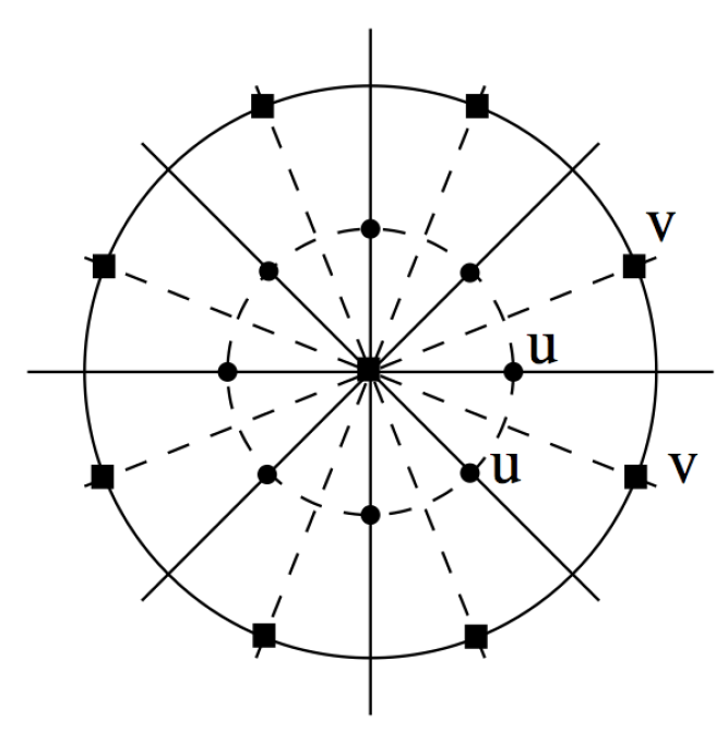
Abbildung 1: Schematic depicting arrangement of winds around a pole in the latitude-longitude grid. Zonal wind components, $u$, are used to determine a horizontal wind vector at the pole, using a least-squares best fit to an assumed solid-body rotation.

2 Test Cases

As part of our project to model exoplanets we have installed the externally released UM VN7.9, using the ND dynamical core and VN8.2, adapted to use the developmental ENDGame dynamical core. We have, in order to check the veracity of our version of the code and test regimes approaching our target systems of hot Jupiters, then run each version through a set of test cases. These test cases isolate the dynamical core and solve for the atmosphere only, in the absence of orography. The test cases presented in this work are the original (simple) Held-Suarez test (HS, Held and Suarez, 1994), a simple Earth-Like test case including a stratosphere (EL, Menou and Rauscher, 2009) and a hypothetical tidally locked Earth, allowing the opportunity to explore the model performance with a longitudinal temperature contrast (TLE, Merlis and Schneider, 2010; Heng et al., 2011b).

For these tests radiative transfer is parameterised using simple temperature forcing to a prescribed temperature profile or ‘Newtonian cooling’, and the heating rate is therefore set by the Newtonian heating rate, $Q_{\rm Newton}$. Practically, however, the codes uses potential temperature as a prognostic, thermodynamic variable and therefore the heating rate is prescribed by

$$Q=Q_{\rm Newton}=-\Pi\left(\frac{\theta-\theta_{\rm eq}}{\tau_{\rm rad}}\right),$$ (5)

where $\tau_{\rm rad}$ the characteristic radiative or relaxation timescale and can be set as constant or as a function of position (latitude) and pressure or height. $\theta_{\rm eq}$ is the equilibrium potential temperature and is derived from the equilibrium temperature profile ($T_{\rm eq}$) using

$$\theta_{\rm eq}^{i}=\frac{T_{\rm eq}}{\Pi^{i}},$$ (6)

where superscript $i$ denotes the current timestep. Practically, the potential temperature is adjusted explicitly within the semi–Lagrangian scheme using

$$\theta^{i+1}=\theta_{D}^{i}-\frac{\Delta t}{\tau_{\rm rad}}\left(\theta^{i}-\theta_{\rm eq}^{i}\right)_{D},$$ (7)

where the superscript $i+1$ denotes the next timestep and $\Delta t$ is the length of the timestep. The subscript $D$ denotes a quantity at the departure point of the fluid element (see explanation in Section 1.2 and Wood et al., 2013, for a full discussion) . Boundary layer friction is also represented using a simple ‘Rayleigh friction’ scheme, where the horizontal winds are damped close to the surface (again explicitly),

$$u^{i+1}=u^{i}-\frac{\Delta t}{\tau_{\rm fric}}u^{i},\\$$ (8)

(and similarly for $v$) where $\tau_{\rm fric}$ is the characteristic friction timescale, and as with $\tau_{\rm rad}$ can be a constant or a function of position and pressure or height. Therefore, each test case prescribes three ‘profiles’: an equilibrium temperature, relaxation or radiative timescale and horizontal frictional timescale profile.

Finally, each simulation has also been run including a very simple dry static adjustment of $\theta$ to remove any convective instability. As the condition for convective instability is $\frac{d\theta}{dz}<0$, each column is examined for negative vertical potential temperature gradients after each timestep. If a column is found to be convectively unstable $\theta(z)$ is re-arranged, i.e. the temperature in the column is just rearranged to ensure stability. Practically, this routine only operates over the pole where the atmosphere can become unstable to convection. The original Held–Suarez test does not include a dry static adjustment scheme, and the atmosphere is close to being neutrally stable over the poles, meaning our results will differ slightly. However, the effect of including a convective adjustment scheme has been explored for several Earth–like test cases by Heng et al. (2011a), and been shown to be negligible.

2.1 Models run

We have run each test case using ND and ENDGame. We have also run each test case using ENDGame but varying the set of simplifications or assumptions to the dynamical equations. Table 2 shows the names we use to refer to different model setups, the dynamical core used, the underlying equation set and the associated approximations (the approximations are as discussed in Section 1.1.1 and presented in Table 1).

Tabelle 2: Table showing the name used in this work with the dynamical core, the name for the equation set (as described in White et al., 2005) and the main included assumptions. For a full description of the underlying equations see White et al. (2005)

Short–Name	EGsh	EGgc	EG	ND
Dynamical core	ENDGame	ENDGame	ENDGame	New Dynamics
White et al. (2005) equation set	NHS	NHD	NHD	NHD
Spherical geopotentials	Yes	Yes	Yes	Yes
Constant gravity	Yes	Yes	No	Yes
‘Shallow–atmosphere’	Yes	No	No	No

The model EG_gc setup was chosen explicitly to match the ND equations, and thereby allow us to potentially isolate differences in solution caused by changes in the numerical scheme between the dynamical cores. These runs are compared and discussed for each test case in turn, alongside comparison to the original test, in this section. These practical tests complement the analysis of normal modes in Thuburn et al. (2002a, b), and standardised flow tests (e.g. Ullrich et al., 2013; Wood et al., 2013). The general parameters for the model runs are listed in Table 3.

Tabelle 3: Table showing the general parameters adopted for the calculations. G72N45 is notation for 144 longitude points and 90 latitude points and $N_{\rm z}$ is the number of vertical levels. T_init is the temperature adopted for our initial hydrostatically stable isothermal atmosphere (as explained in Section 2.2.1) and $\Delta T_{\rm sample}$ is the temporal distance between model outputs.

Parameter	Value
Horizontal Resolution	G72N45
Nz	32
Timestep (s)	1200
Tinit (K)	264
$\Delta T_{\rm sample}$ (days)	10
Temporal weighting, $\alpha$	0.7 (ND), 0.55 (EG)

2.2 Vertical coordinate & methods of model comparison

The literature sources which we compare our results with all used GCMs which adopt pressure or $\sigma$ as their vertical coordinate ($\sigma=\frac{p}{p_{\rm surf}}$, where $p_{\rm surf}$ is the surface pressure), whereas the UM is height-based (the MCore is another example of a dynamcial core adopting a height–based coordinate, see Ullrich and Jablonowski, 2012, for a description). This creates some barriers to a clean comparison between our models and the literature examples. Firstly, the boundary conditions (and therefore model domain) can only be approximately matched. Secondly, our vertical resolutions, and more specifically, level placements will be different. Finally, to explicitly compare the results we must transform our results to $\sigma$ space.

Our upper boundary, being constant in height, will experience fluctuations in pressure. Practically, the initial pressure of the inner boundary (or surface) is set and a domain large enough so as to reach the lowest required pressure is selected. Therefore, if the horizontal or temporal pressure gradients are significant our model domain will not match that of a pressure based model, where the upper boundary is a constant pressure surface. While this is not the case for the tests in this work, for our work on hot Jupiters changes in the pressure on the top boundary can lead to a significant change in the physical size of the domain (Mayne et al, submitted). The distribution of levels within our domain can then be selected to sample the associated $\sigma$ space evenly to match the literature models. Practically, for each test case we run a model with a (moderate resolution) uniform grid over a domain extending to pressures lower than sampled in the original, literature, $\sigma$ model. Zonal and temporal averages are then used to create a set of level heights (and an upper boundary position) to emulate even $\sigma$ sampling. We have also, when compared to the literature models we examine, increased our number of vertical levels to ensure sufficient resolution. The resulting level heights for each test case are presented in Table A.2 in dimensionless height coordinates, alongside the approximate $\sigma$ value of each level.

Comparison of our models with literature results then requires additional conversion. Although our level and boundary placements have been selected to better sample the required $\sigma$ space we still use geometric height as our vertical coordinate. Therefore, for each completed test case, the pressure (and therefore $\sigma$) values are found and the prognostic variable is interpolated (at every output timestep) into $\sigma$ space.

To determine a satisfactory match of the mean, large–scale, long term structure of our modeled atmospheres with literature results, we compare the prognostic fields of velocity and temperature. These fields are averaged (using a mean) in the diagnostic plots of the original publications in both time and space. Additional care must be taken when performing spatial averaging and comparing models across different vertical coordinates (as discussed in the Appendix of Hardiman et al., 2010). Where we are comparing directly to a literature figure or result we perform the spatial averaging in $\sigma$ space. The required prognostic field is (as discussed above) interpolated from the height grid onto a $\sigma$ grid, and then the average performed along constant $\sigma$ surfaces, to allow the most consistent comparison with literature, $\sigma$–based models. To further enhance the comparison of our results with those in the literature, where possible the line contours (solid lines for positive values and dotted lines for negative) presented in the plots of our model results have been chosen to match the original publications. We have then, to aid a qualitative interpretation of our models, complemented the line contours with additional (more numerous) colour contours. For plots showing wind or circulation patterns the coloured contours are separated at zero (where blue represents negative flow, and red positive), again to aid visual presentation of the flow. Each of the original publications introducing the tests we have performed include the comparison of additional quantities (for example the eddy temperature and wind variance in Held and Suarez, 1994). In this work, however, for brevity (as we are performing several tests) we compare only the prognostic variable fields, i.e. wind and temperature, complemented by comparison of the Eddy Kinetic Energy (EKE) defined as

$${\rm EKE}=\frac{\left(u^{\prime 2}+v^{\prime 2}\right)}{2},\\$$ (9)

where the prime denotes a perturbation such that $u^{\prime}=u-\overline{u}^{\lambda_{\rm z},t}$, where $\overline{u}^{\lambda_{\rm z},t}$ is the variable averaged (mean) in longitude ($\lambda$) and time ($t$). One critical difference with this quantity (compared to the others we plot) however, is that the spatial (zonal) average is performed in height coordinates (hence the subscript $z$). Therefore, plots of EKE will be presented in height not $\sigma$ space. This is done as we compare the zonal and temporal mean of the EKE, i.e. $\overline{{\rm EKE}}^{\lambda_{\rm z},t}$. Given that the perturbation itself is constructed from a spatial and temporal mean, we are performing several averaging processes and it is simpler and more intuitive to keep the variable in the natural coordinate system of the model. Moreover, in the case of EKE, we are actually comparing only our own models with each other, not with a literature $\sigma$-based model. The EKE then allows us to explore differences in the eddy structures of the models, complementary to the plots depicting the relatively insensitive means of the wind and temperature fields. Additional details regarding the comparison between our work and that of Heng et al. (2011b) can be found in Appendix A.1.

2.2.1 Initial conditions

As stated in Held and Suarez (1994), for their HS test an initial spin–up time of 200 days is used to effectively allow the system to reach a statistically steady–state and erase the initial conditions. This is why temporal average (whenever it is stated as being performed) means the average of the field from 200 to 1200 days. Our adopted initial conditions were a simple, hydrostatically balanced, isothermal atmosphere (temperature presented in Table 3) with zero $u$,$v$ and $w$ velocities.

2.3 Held–Suarez

The HS test prescribes an equilibrium temperature profile of

$$T_{\rm eq}={\rm max}\{T_{\rm stra},T_{\rm HS}\},\\$$ (10)

where,

$$T_{\rm HS}=\\ \left[T_{\rm surf}-\Delta T_{\rm EP}\sin^{2}\phi-\Delta T_{z}\ln\left(\frac{p}{p_{0}}\right)\cos^{2}\phi\right]\left(\frac{p}{p_{0}}\right)^{\kappa},$$ (11)

and, $T_{\rm stra}=200$ K, $T_{\rm surf}=315$ K, $\Delta T_{\rm EP}=60$ K, $\Delta T_{z}=10$ K and $p_{0}=1\times 10^{5}$ Pa. The radiative timescale is modeled as,

$$\frac{1}{\tau_{\rm rad}}=\\ \frac{1}{\tau_{\rm rad,d}}+\begin{cases}0\mbox{,}\,&\sigma\leq\sigma_{\rm b}\mbox{,}\\ \left(\frac{1}{\tau_{\rm rad,u}}-\frac{1}{\tau_{\rm rad,d}}\right)\left(\frac{\sigma-\sigma_{\rm b}}{1-\sigma_{\rm b}}\right)\cos^{4}\phi\mbox{,}\,&\sigma>\sigma_{\rm b}\mbox{,}\end{cases}$$ (12)

where, $\tau_{\rm rad,d}=40$ days, $\tau_{\rm rad,u}=4$ days and $\sigma_{\rm b}=0.7$ (the top of the surface friction boundary layer).

The boundary layer horizontal wind damping enforces a damping on a timescale, $\tau_{\rm fric}$ given by:

$$\frac{1}{\tau_{\rm fric}}=\begin{cases}0\mbox{,}\,&\sigma\leq\sigma_{\rm b}\mbox{,}\\ \left(\frac{1}{\tau_{\rm fric,f}}\right)\left(\frac{\sigma-\sigma_{\rm b}}{1-\sigma_{\rm b}}\right)\mbox{,}\,&\sigma>\sigma_{\rm b}\mbox{,}\end{cases}$$ (13)

where, $\tau_{\rm fric,f}=1$ day.

Figures 2 and 3 show the zonally (along constant $\sigma$ surfaces) and temporally averaged zonal wind and temperature ($\overline{u}^{\lambda_{\sigma},t}$ and $\overline{T}^{\lambda_{\sigma},t}$), respectively, from the original (Held and Suarez, 1994) publication, and from our ND and ENDGame setups.

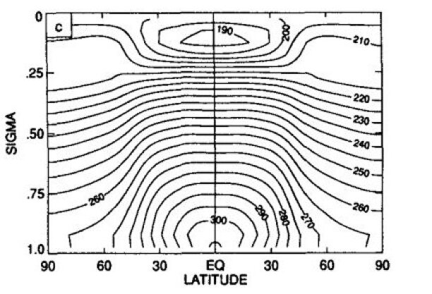
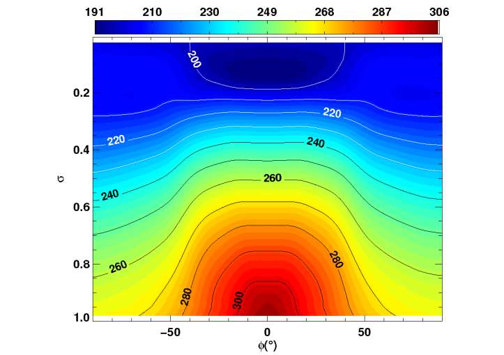
Abbildung 2: Figure showing, for the Held–Suarez test (Held and Suarez, 1994), the zonally and temporally averaged (i.e. mean from 200 to 1200 days, see Section 2.2.1) temperature (K) as a function of latitude and $\sigma$. Top panel: original finite difference model Figure 1 from Held and Suarez (1994), (c) American Meteorological Society. Used with permission. Middle panel: ND version. Bottom Panel: EG version (see Table 2 for explanation of model types).

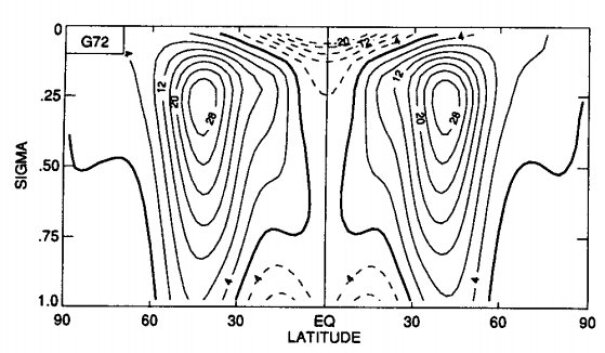
Abbildung 3: Same as Figure 2 but for zonal wind (ms^-1).

Qualitatively, both the ND (middle panel) and the EG (bottom panel) temperature and zonal wind fields (when averaged zonally and temporally) match the original Held and Suarez (1994) (top panel) results of the finite difference model. However, the 210 K contour (Figure 2), and the wind contours extending over the poles, and over the equator (Figure 3) show a slightly better match with Held and Suarez (1994) when moving from the ND to the ENDGame models (however these flows represent very small velocities $\lesssim 1$ ms^-1). The ND model shows a slightly different vertical temperature profile for the lowest levels, when compared to the EG model. This is caused by differences in the temperature modeled in the lowest grid cell. The ENDGame model records the temperature, in the atmosphere array, down to the surface, whereas ND does not. Therefore, for display purposes the potential temperature across the bottom cell has been estimated to be constant in the ND model, resulting in a slight increase of temperature (as $T=\Pi\theta$ and the lowest $\sigma\sim 0.97$, and by definition $\sigma_{\rm surf}\equiv 1$, see Table A.2).

Figure 4 shows zonally and temporally averaged zonal wind plots for all of the ENDGame models (namely, EG, EG_gc and EG_sh, where EG has been presented already in Figure 3 but is reproduced in Figure 4 to aid visual comparison). The similarity of the panels of Figure 4 shows that, as expected for such a domain and flow regime (i.e. the lack of large, in vertical extent, circulation cells), making the ‘shallow–atmosphere’ approximation (or approximating gravity as a constant only) does not significantly affect the resulting long–term large–scale flow. There is tentative evidence, if one scrutinises the flow over the pole, for the subsequent simplification of the model moving it towards the Held and Suarez (1994) result, however, the velocities in these regions are small ($<1$ ms^-1). These results also match the spectral and grid–based models of Heng et al. (2011b) (see Figures 1 & 2 of Heng et al., 2011b). Another important point to note is that in Held and Suarez (1994) the model was run using 20 vertical levels. We have adopted 32 vertical levels, and the agreement between our results and those of Held and Suarez (1994) is a promising indication that we have used sufficient resolution.

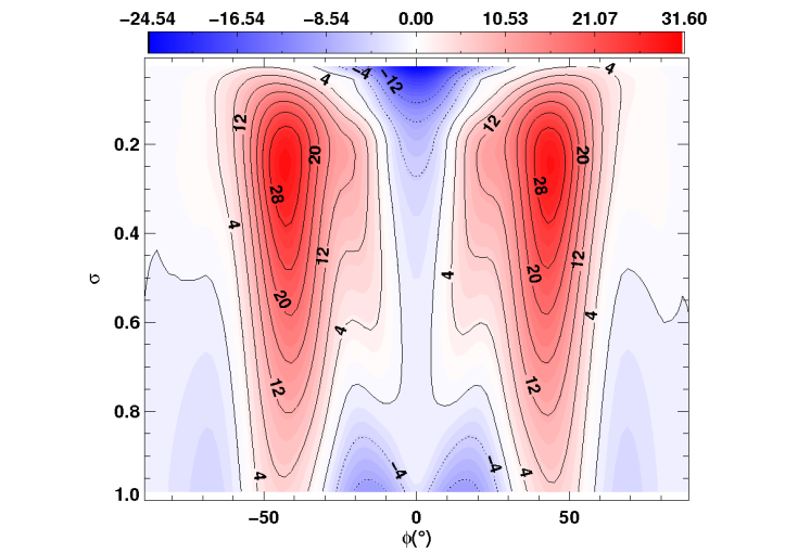
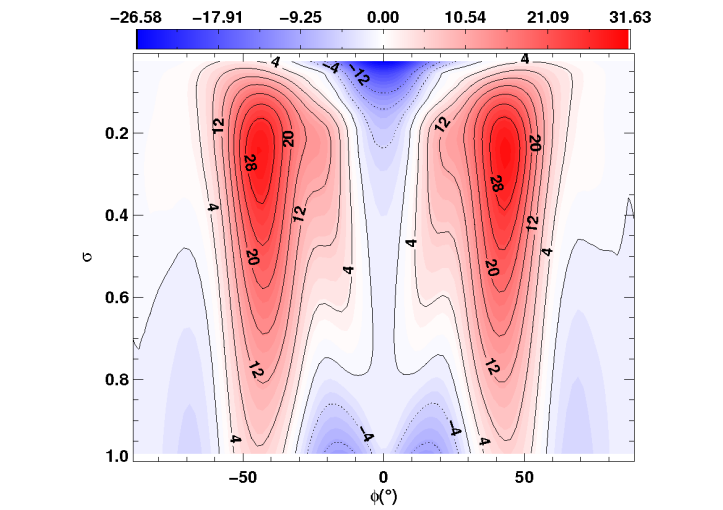
Abbildung 4: Figure, for the Held–Suarez test (Held and Suarez, 1994), showing the zonally and temporally averaged zonal wind (ms^-1) as a function of latitude and $\sigma$. Top panel: EG model (also shown in Figure 3 but reproduced here to aid comparison). Middle panel: EG_gc model. Bottom panel: EG_sh model (see Table 2 for explanation of model types).

Figure 5 shows, explicitly, the differences between the temperature and wind structures between the EG and ND models, i.e. EG$-$ND from Figures 2 and 3 as the top and bottom panels, respectively. Similar plots have been constructed for EG$-$EG_gc and EG$-$EG_sh but the differences are negligible ($\Delta T\lesssim 1$ K and $\Delta u\lesssim 2.5$ ms^-1).

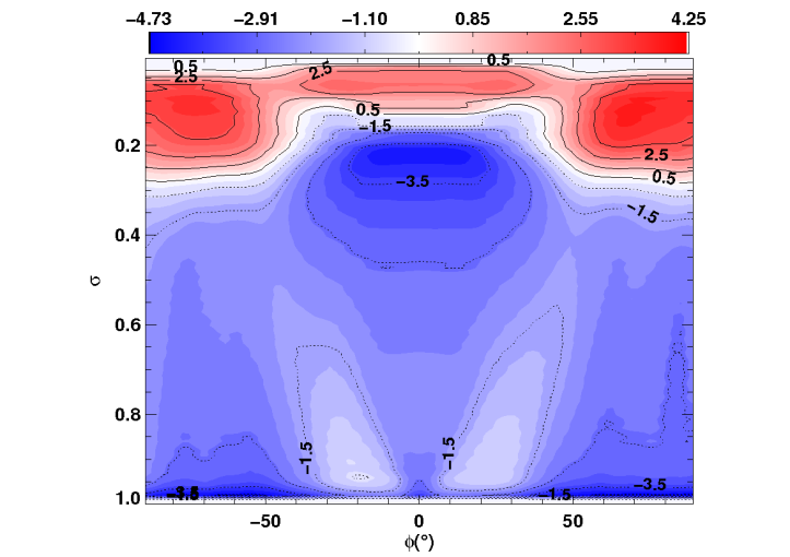
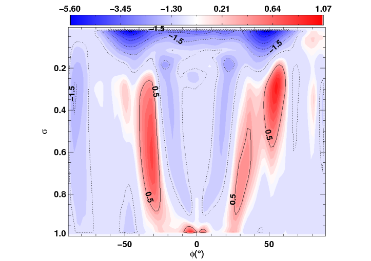
Abbildung 5: Figure, for the Held–Suarez test (Held and Suarez, 1994), showing the differences EG$-$ND of the zonally and temporally averaged zonal temperature (K), top panel, and wind (ms^-1), bottom panel (see Table 2 for explanation of model types).

Figure 5 shows that the ND model has a cooler upper atmosphere than the EG model (top panel), and a warmer lower atmosphere, although the differences are only $\sim 3$ K. The prograde jets in the EG model are faster than those in the ND model, and the retrograde flow in the upper atmosphere is enhanced (bottom panel of Figure 5), however, the changes are small $\sim 1$ ms^-1.

Figures 2, 3, 4 and 5 show that the overall large–scale, long–term flow for the HS test case are relatively consistent both across all of our models, and with literature results (only modest departures are evident in the wind and temperature structures of the atmosphere). The diagnostics used i.e. zonal and temporally averaged prognostic variables are, however, relatively insensitive. Therefore, as discussed in Section 2.2 we now explore the EKE found in each model to illustrate differences in the eddy component of the flow.

Figure 6 shows the EKE as defined in Section 2.1, zonally (along geometric height surfaces) and temporally averaged ($\overline{{\rm EKE}}^{\lambda_{\rm z}t}$) as a function of height (m) and latitude (^∘), for the ND and all ENDGame models. Figure 6 shows excellent agreement of the EKE for all of the models. However, a greater peak level of EKE associated with the EG_sh model, and the least with the EG_gc model. Overall, the structures of the plots are very similar for all models. However, the results of the ND model shows, with respect to the ENDGame plots, an increase in the EKE at $\phi\sim 50^{\circ}$ towards the upper boundary (i.e. coincident with the peak wind speed of the prograde jets). To illustrate the difference explicitly we show in Figure 7, as with the temperature and zonal wind fields, the differences of the $\overline{{\rm EKE}}^{\lambda_{\rm z}t}$ for each model. Specifically, Figure 7 shows difference in $\overline{{\rm EKE}}^{\lambda_{\rm z}t}$ in the sense EG$-$ND, EG$-$EG_gc and EG$-$EG_sh, as the top, middle and bottom rows respectively. In Figure 7 the line contours have been chosen to be the same for all panels.

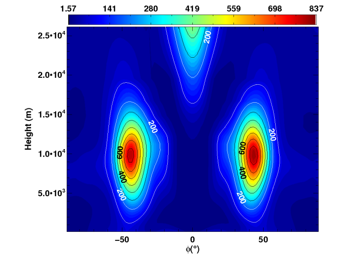
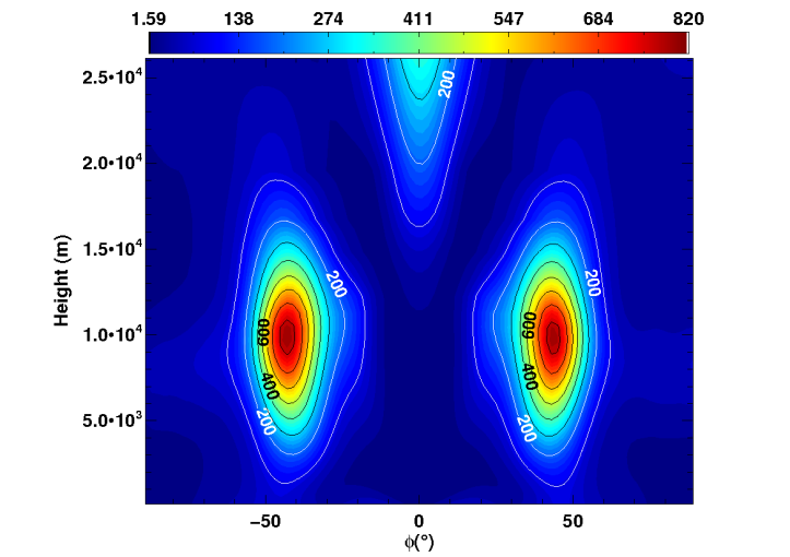
Abbildung 6: Figure, for the Held–Suarez test (Held and Suarez, 1994), showing the zonally (in geometric height) and temporally averaged Eddy Kinetic Energy (EKE, see Section 2.1) as a function of latitude and height. Top left panel: ND, top right panel: EG_sh, bottom left panel: EG_gc and bottom right panel: EG models (see Table 2 for explanation of model types). Note the contours (solid lines) are the same in all plots.

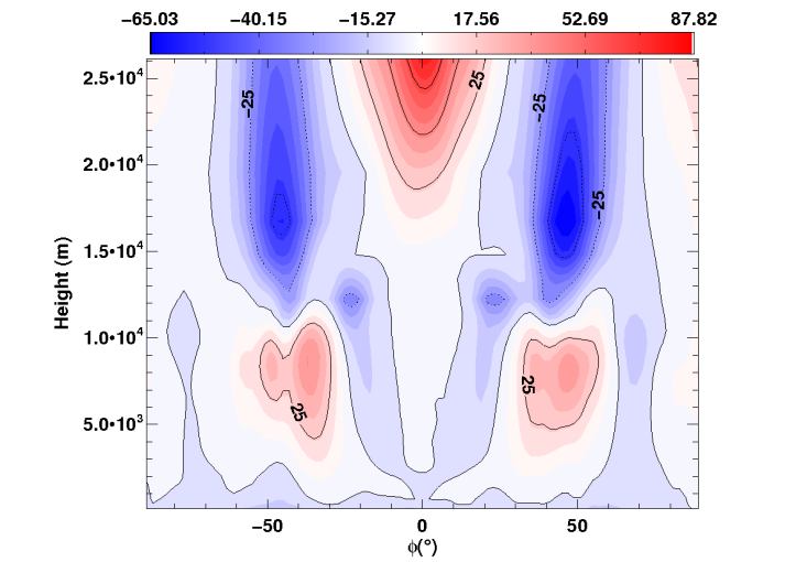
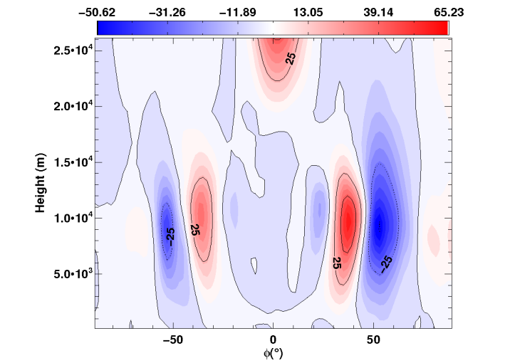
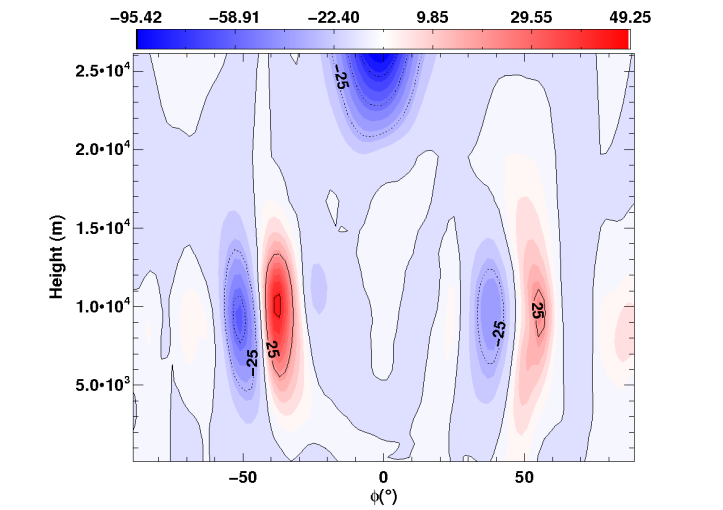
Abbildung 7: Figure, for the Held–Suarez test (Held and Suarez, 1994), showing the differences EG$-$ND (top), EG$-$EG_gc (middle) and EG$-$EG_sh (bottom), of the zonally and temporally averaged EKE. The line contours are the same for all panels (see Table 2 for explanation of model types).

Figure 7 shows, for the EG model compared to ND (top panel), more kinetic energy associated with the eddy component of the flow over the equator, and near the surface at a latitude associated with the peak zonal wind speed ($\phi\sim 50^{\circ}$). The magnitude of the peak relative differences in $\overline{{\rm EKE}}^{\lambda_{\rm z}t}$ are $\sim$1.65, 0.36 and 0.42 for the differences EG$-$ND, EG$-$EG_gc and EG$-$EG_sh, respectively. There is a decrease in EKE found in the EG model when compared to the ND model higher in the atmosphere. Comparing EG to EG_gc (middle panel) again shows more kinetic energy associated with eddies in the EG model, over the equator, at high altitudes, however, the differences associated with the mid–latitude jets now appear over similar altitudes. Finally, the difference EG$-$EG_sh (bottom panel) shows a similar spatial pattern to EG$-$EG_gc but the signs are reversed. Overall, Figure 7 shows that detailed, eddy, component of the flow, can be quite different, although not affecting the diagnostic plots (for example Figures 2 and 3) significantly.

2.4 Earth-Like

For the Earth-Like test case of Menou and Rauscher (2009), the temperature profile includes a parameterised stratosphere,

$$T_{\rm eq}=T_{\rm vert}+\beta_{\rm trop}\Delta T_{\rm EP}\left(\frac{1}{3}-\sin^{2}\phi\right)\\$$ (14)

where

$$T_{\rm vert}=\begin{cases}T_{\rm surf}-\Gamma_{\rm trop}(z_{\rm stra}+\frac{z-z_{\rm stra}}{2})\\ +\left(\left[\frac{\Gamma_{\rm trop}(z-z_{\rm stra})}{2}\right]^{2}+\Delta T_{\rm strat}^{2}\right)^{\frac{1}{2}}\mbox{,}\,&z\leq z_{\rm stra}\mbox{,}\\ T_{\rm surf}-\Gamma_{\rm trop}z_{\rm stra}+\Delta T_{\rm strat}\mbox{,}\,&z>z_{\rm stra}\mbox{,}\end{cases}$$

and $T_{\rm surf}=288$ K is the surface temperature, $\Gamma_{\rm trop}=6.5\times 10^{-3}$ Km^-1 is the lapse rate, and $\Delta T_{\rm strat}=2$ K, an offset to smooth the transition from the troposphere (finite lapse rate) to the isothermal stratosphere. $z_{\rm stra}$ and $\sigma_{\rm stra}$ are then the locations in height and $\sigma$ of the tropopause. $\beta_{\rm trop}$ is defined as

$$\beta_{\rm trop} =\begin{cases}\sin\frac{\pi(\sigma-\sigma_{\rm stra})}{2(1-\sigma_{\rm stra})}\mbox{,}\,&z\leq z_{\rm stra}\,\mbox{ or }\,\sigma\geq\sigma_{\rm stra}\mbox{,}\\ 0\mbox{,}\,&z>z_{\rm stra}\,\mbox{ or }\,\sigma<\sigma_{\rm stra}\mbox{.}\end{cases}$$

The remaining parameters match those of HS, except, here the radiative timescale is set as a constant, $\tau_{\rm rad}=15$ days, but, following Heng et al. (2011b) the same ‘Rayleigh friction’ scheme as for HS is implemented (this differs from the choice of Menou and Rauscher, 2009, where only the bottom level winds are damped which creates a resolution dependent damping profile).

Figure 8 shows the zonally averaged (in $\sigma$ space) zonal wind and temperature fields for our ND and EG models, and the results from Heng et al. (2011b), both have been temporally averaged (i.e. $\overline{u}^{\lambda_{\sigma},t}$ and $\overline{T}^{\lambda_{\sigma},t}$). Our models are in excellent agreement with the results of Heng et al. (2011b) (although we have slightly stronger high–altitude components of the mid–latitude jets). Our results also match the ‘snapshots’ of the flow field presented in Menou and Rauscher (2009). This agreement again, as found with the HS test, suggests sufficient vertical resolution (15, 20 and 32 vertical levels used in Menou and Rauscher, 2009; Heng et al., 2011b, and this work, respectively).

Further evidence of the extrapolation of the temperature down to the surface of the ND model, performed as part of the visualisation process, is apparent in the right panels of Figure 8, in the contours close to the surface. The left panels of Figure 8 shows a slight improvement in the agreement of the flow structure at high and low latitudes, between the results of Heng et al. (2011b) and our own model when moving from ND to EG. Figure 9 then shows the temporally and zonally averaged zonal wind for the three versions of the ENDGame models. The qualitative agreement between all the panels in Figure 9 again shows that the assumptions are valid, and that the code is consistently solving for the long–term and large–scale 3D flow. There are only very slight differences, for example, as we move towards a more simplified model (i.e. downwards in Figure 9) we generally see the edge of 3.6 ms^-1 contour moving to higher latitudes, and a slight degradation in the symmetry of the flow. Additionally, all of the ND and ENDGame models show a greater hemispherical symmetry in the wind patterns than the finite difference model presented in Heng et al. (2011b), and, in fact, match the levels of symmetry present in the results of the spectral code of Heng et al. (2011b) (not shown here).

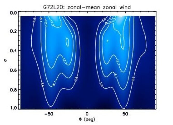
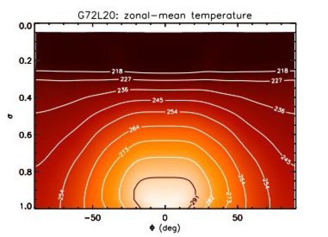
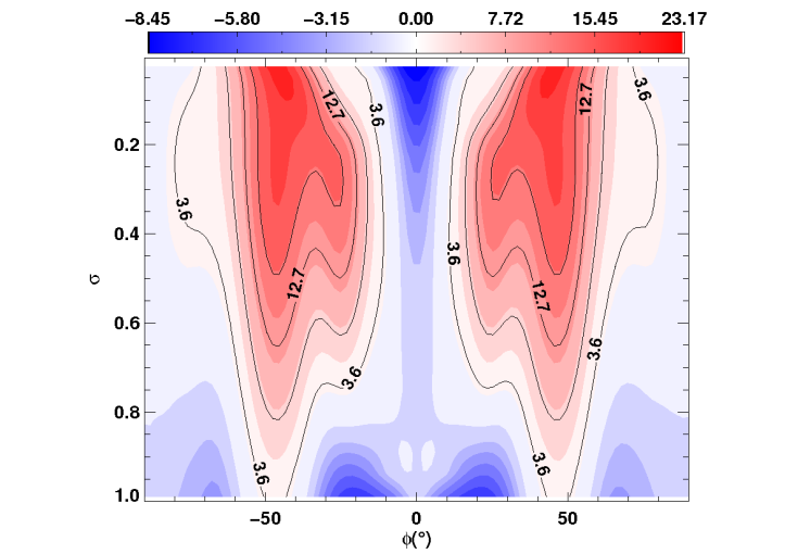
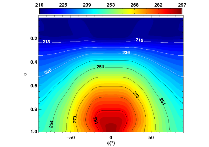
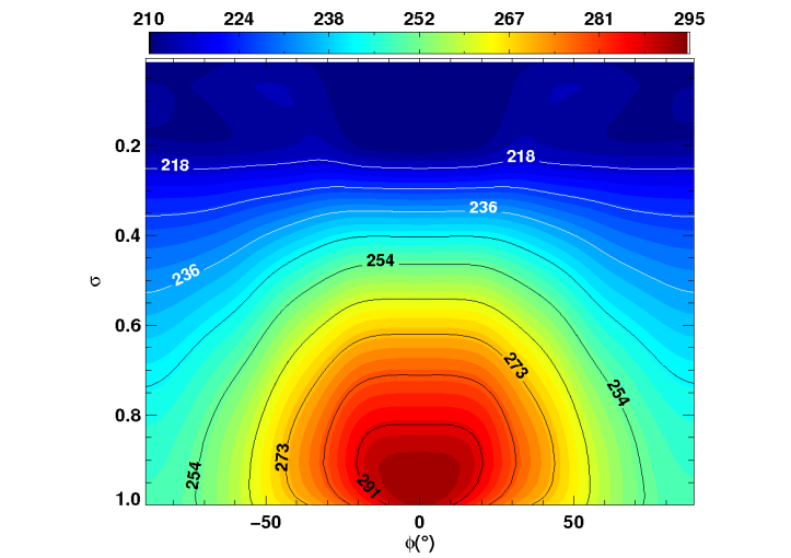
Abbildung 8: Figures showing, for the Earth–Like test (Menou and Rauscher, 2009), the zonally averaged temperature and zonal wind. Top panels: temporally averaged results from grid–based model of Heng et al. (2011b) (reproduced by permission of Oxford University Press). Middle and bottom panels: temporally averaged results from this work using the ND and EG models, respectively (see Table 2 for explanation of model types).

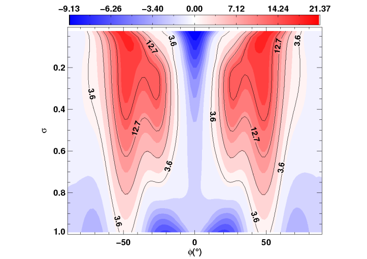
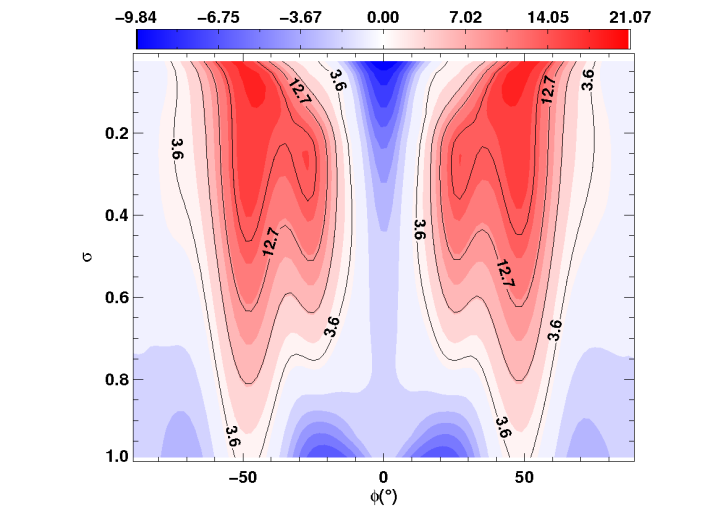
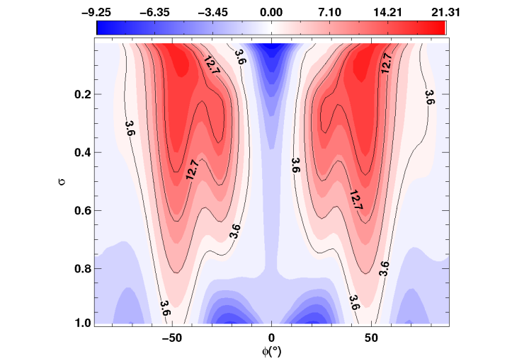
Abbildung 9: Figures showing, for the Earth–Like test (Menou and Rauscher, 2009), the zonally and temporally averaged zonal wind fields for the different EG models. Top panel:, EG, middle panel:, EG_gc and bottom panel:, EG_sh (see Table 2 for explanation of model types).

Again, as with the HS test case in Section 2.3 the different ENDGame models show negligible differences in the results, so only the difference EG$-$ND is shown in Figure 10. The format of Figure 10 matches that of Figure 5. Figure 10 shows a similar, yet reduced in magnitude, pattern to that present in Figure 5, with a warmer upper atmosphere showing enhanced flow, and cooler mid–atmosphere, in the EG model over the ND model. The zonal jets have also shifted closer to the poles in the EG model. This is caused, largely, by the adverse effects of the polar filtering used in the ND model (when polar filtering is applied to the EG model the jets move closer to the location found for ND).

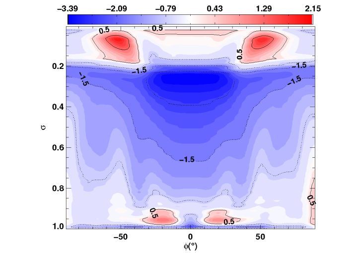
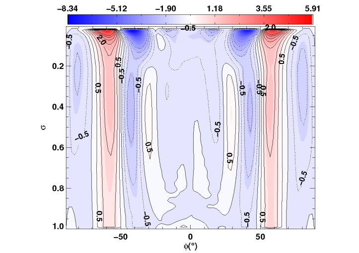
Abbildung 10: Figure, for the Earth–Like test (Menou and Rauscher, 2009), showing the differences EG$-$ND of the zonally and temporally averaged temperature, top, and zonal wind (ms^-1) bottom panel (see Table 2 for explanation of model types).

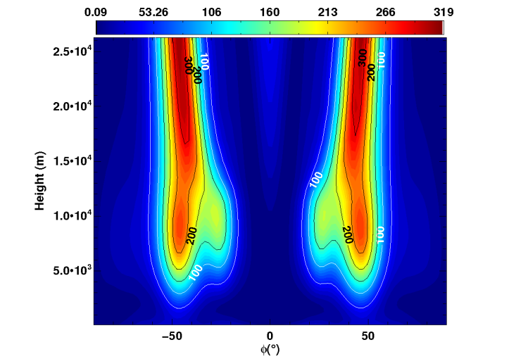
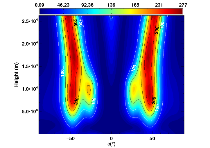
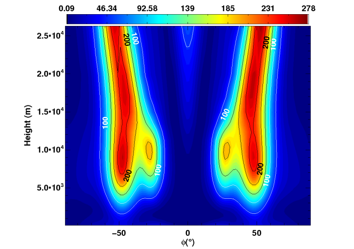
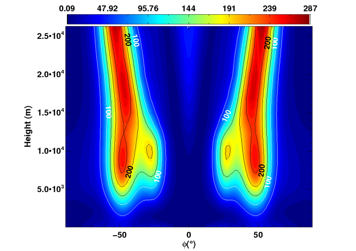
Abbildung 11: Figure, for the Earth–Like test (Menou and Rauscher, 2009), showing the zonally (in geometric height) and temporally averaged Eddy Kinetic Energy (EKE, see Section 2.1) as a function of latitude and height. Top left panel: ND, top right panel: EG_sh, bottom left panel: EG_gc and bottom right panel: EG models (see Table 2 for explanation of model types). Note the contours (solid lines) are the same in all plots.

Again, to explore the eddy component of the flow, Figure 11 shows the EKE, zonally (along geometric height surfaces) and temporally averaged ($\overline{{\rm EKE}}^{\lambda_{\rm z}t}$), for the ND and all ENDGame models. Figure 11, as in Figure 6 shows qualitative agreement with the overall pattern of $\overline{{\rm EKE}}^{\lambda_{\rm z},t}$, however in this case the peak value is much larger for the ND model (compared to any ENDGame model).The magnitude of the peak relative differences in $\overline{{\rm EKE}}^{\lambda_{\rm z}t}$ are $\sim$2.0, 0.80 and 0.46 for the differences EG$-$ND, EG$-$EG_gc and EG$-$EG_sh, respectively, slightly larger than found in the HS case. The ENDGame models also show more structure along the peak of $\overline{{\rm EKE}}^{\lambda_{\rm z},t}$ activity and the ‘lobes’ equator ward of the peak.

To emphasise the slight differences in $\overline{{\rm EKE}}^{\lambda_{\rm z},t}$ apparent in Figure 11 we present a difference plot, for EG$-$ND only (as the differences between the ENDGame models are an order of magnitude smaller), in Figure 12.

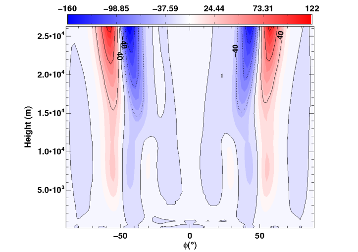
Abbildung 12: Figure, for the Earth–Like test (Menou and Rauscher, 2009), showing the differences EG$-$ND of the zonally and temporally averaged EKE (see Table 2 for explanation of model types).

There is a significant reduction in variation in the $\overline{{\rm EKE}}^{\lambda_{\rm z},t}$ across all of the EL models, when compared to the HS test case (see Figures 6 and 11), as the EL test is a simpler flow regime to capture. The EG$-$ND of $\overline{{\rm EKE}}^{\lambda_{\rm z},t}$, in Figure 12 also shows the peak difference is close to the upper boundary, coincident in latitude, with the peak of the prograde jets. As seen in Figure 10 a shift in the latitudinal location of the pattern is observed between the EG and ND models. As before, this is due to the polar filtering applied in the ND model.

2.5 Tidally Locked Earth

For the Tidally Locked Earth (TLE) test of Merlis and Schneider (2010) we slow the rotation rate so that a day is now equal to an orbital period (i.e. a year), $\Omega\to\frac{\Omega}{365}$. This introduces a longitudinal temperature contrast and allows us to test the model behaviour in a familiar system (i.e. Earth) but incorporating aspects found in the hot Jupiter atmospheric regime. We have not included moisture in the calculation and therefore, have essentially, performed the simplified version of the test which is described and performed by Heng et al. (2011b). The equilibrium temperature profile is then a modified version of the HS profile, enforcing a longitudinal temperature contrast and ‘hot spot’ at the subsolar point centred at a longitude of $180^{\circ}$ (and latitude of zero). It is given by:

$$T_{\rm eq}={\rm max}\{T_{\rm stra},T_{\rm TLE}\},\\$$ (17)

where,

$$T_{\rm TLE}=\\ \left[T_{\rm surf}+\Delta T_{\rm EP}\cos(\lambda-180^{\circ})\cos\phi-\Delta\theta_{z}\ln\left(\frac{p}{p_{0}}\right)\cos^{2}\phi\right]\\ \left(\frac{p}{p_{0}}\right)^{\kappa}.\\$$ (18)

The parameters and values in common with the HS model take the same values.

However, for this model, where significant flow over the pole exists, we must add a sponge layer into the ENDGame formulation for model stability (ND incorporates a polar filter). This damps vertical motions and is explained in Klemp and Dudhia (2008); Melvin et al. (2010). The damping term $R_{w}$ (included in the solution for vertical velocity) is,

$$w^{t+\Delta t}=w^{t\*}+S_{w}-R_{w}\Delta tw^{t+\Delta t},\\$$ (19)

where $w^{t}$ and $w^{t+\Delta t}$ are the vertical velocities at the current and next timestep, $S_{w}$ a source term, and $\Delta t$ the length of the timestep (as before). The spatial extent and value of the damping coefficient ($R_{w}$) is then determined by the equation

$$R_{w}=\\ \begin{cases}{\rm C}\left(\sin^{2}\left(0.5\pi(\eta-\eta_{\rm s})\left(\frac{1.0}{1.0-\eta_{\rm s}}\right)\right)+\sin^{40}(\phi)\right)\mbox{,}\,&\eta\geq\eta_{\rm s}\\ 0\mbox{,}\,&\eta<\eta_{\rm s},\\ \end{cases}$$ (20)

where, given the absence of orography, $\eta=\frac{z}{H}$ (i.e. non–dimensional height, where $H$ is the height of the upper boundary), $\eta_{\rm s}$ is the start height for the top level damping (set to $\eta_{\rm s}=0.75$) and $C$ is a coefficient (set to 0.05).

Figure 13 is a reproduction of the grid–based model results for the TLE test in Heng et al. (2011b). It shows the temperature at the $\sigma=0.975$ surface at 1200 days (top panel), the temporally averaged zonal wind ($\overline{u}^{t}$) at the surfaces $\sigma=0.225$, $0.525$ and $0.975$ (in descending panel order).

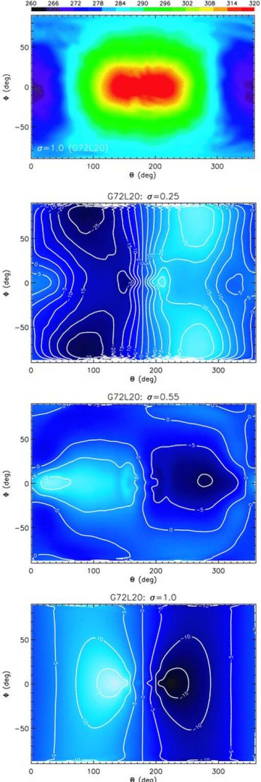
Abbildung 13: Figure reproduced from Heng et al. (2011b) of the results from the grid–based model of the TLE test case (reproduced by permission of Oxford University Press). Showing (from the top panel to the bottom panel) temperature at 1200 days and $\sigma=0.975$, then, temporally averaged zonal wind at $\sigma=0.225$, $0.525$ and $0.975$.

Figure 14 shows the same type of plots as Figure 13, but constructed using the ND (left panels) and EG (right panels) models, where the other ENDGame models are omitted as the results are negligibly different from the EG model.

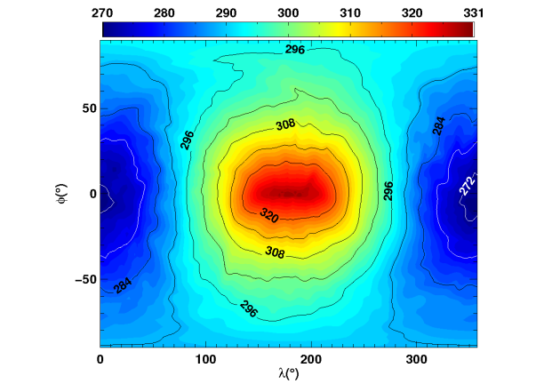
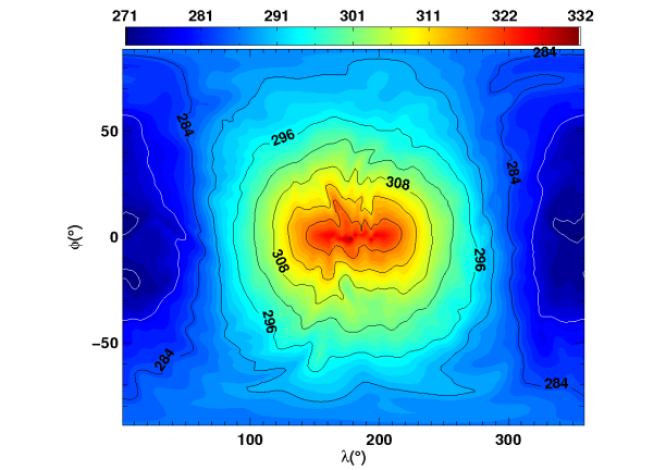
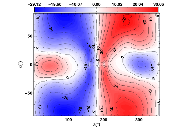
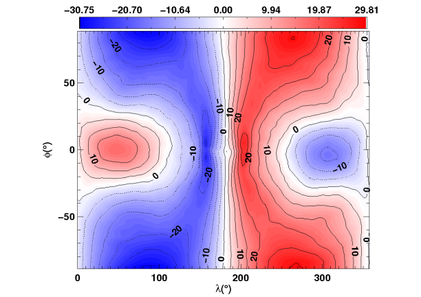
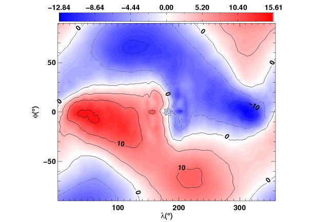
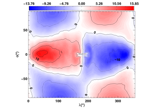
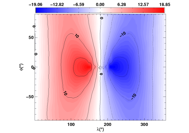
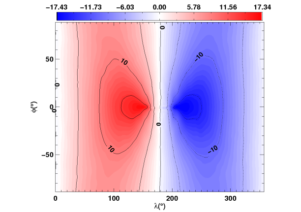
Abbildung 14: Figure showing, for the Tidally Locked Earth test (Merlis and Schneider, 2010; Heng et al., 2011b), (from the top panels to the bottom panels) temperature at 1200 days and $\sigma=0.975$, then, temporally averaged zonal wind at $\sigma=0.225$, $0.525$ and $0.975$. Results are from the ND (left panels) and EG (right panels) models (see Table 2 for explanation of model types).

Figure 15 is a reproduction of the results of the grid–based model for the TLE test case of Heng et al. (2011b), showing the temporally averaged meridional velocity ($\overline{v}^{t}$) at $\sigma=0.225$, $0.525$ and $0.975$ (from top to bottom panel, respectively).

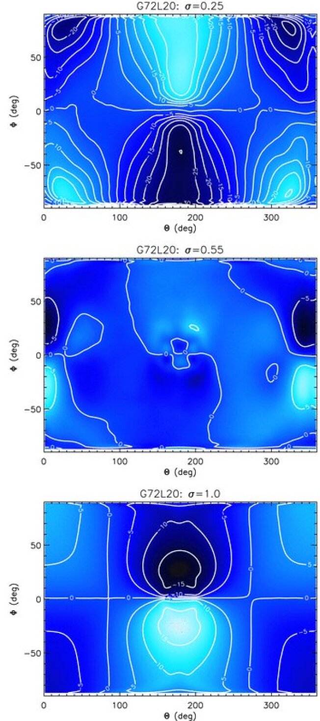
Abbildung 15: Figure reproduced from Heng et al. (2011b) of the results from the grid–based model of the TLE test case (reproduced by permission of Oxford University Press). Showing (from the top panel to the bottom panel) the temporally averaged meridional wind at $\sigma=0.225$, $0.525$ and $0.975$.

The results for our models are shown in Figure 16 in the same vertical format as Figure 15. As for Figure 14 the figures show the ND (left panels) and EG (right panels) models, where (as with Figure 14) the other ENDGame models are omitted as the results are negligibly different from the EG model.

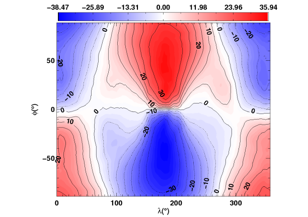
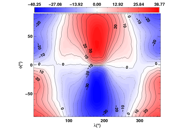
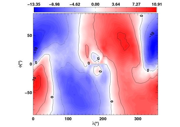
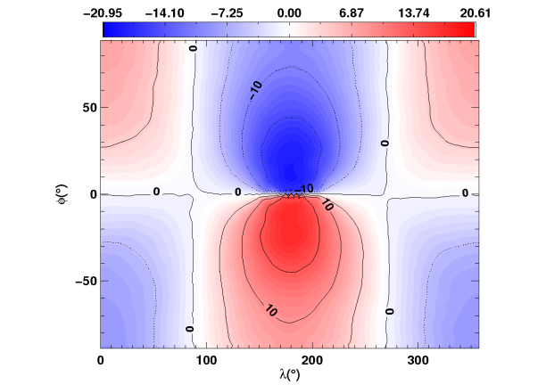
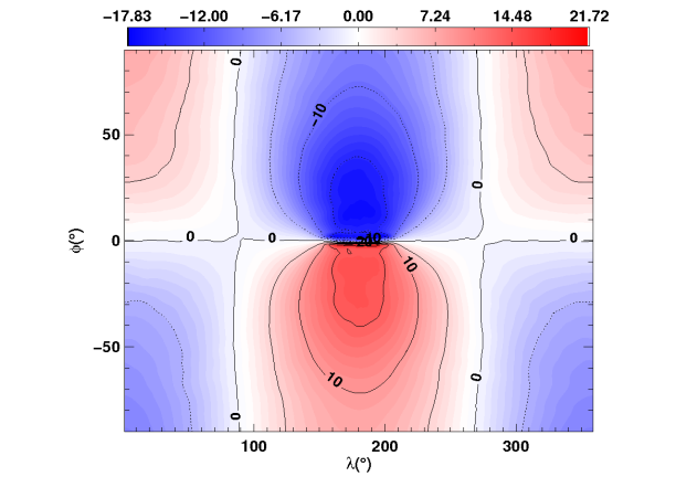
Abbildung 16: Figure showing, for the Tidally Locked Earth test (Merlis and Schneider, 2010; Heng et al., 2011b), (from the top panels to the bottom panels) the temporally averaged meridional wind at $\sigma=0.225$, $0.525$ and $0.975$. Results are from the ND (left panels) and EG (right panels) models (see Table 2 for explanation of model types).

Comparison of the results of Heng et al. (2011b), Figures 13 and 15 with our results, Figures 14 and 16 reveals some disagreement. However, Figures 13 and 15 show results from the finite difference model, and our results agree much more closely with those derived from the spectral code of Heng et al. (2011b) (this is discussed in more detail later in this section). Again, as before our vertical resolution is higher than that of Heng et al. (2011b), 32 as opposed to 20 levels. Tentative evidence for a smoother modeling of the meridional flow can also be seen by comparing our results for the $v$ field (Figure 16) at a $\sigma$ of $0.225$ and $0.525$ to that of Heng et al. (2011b) (Figure 15). Our figures produce flow contours less featured than those of Heng et al. (2011b) (in fact our model matches more closely the spectral model results not reproduced here which we expect to be more accurate for large–scale flows, compared to the finite-difference model). Additionally, as with the previous cases, given the model domain one would expect little difference in results whether the ‘shallow–atmosphere’ approximation is made or not (given the aspect ratio, height over the length scale, $H/L\sim\frac{3.2\times 10^{4}}{2.0\times 10^{7}}\sim 10^{-3}$, where the length scale is chosen as half the perimeter of the planet due to the presence of hemispherical circulation cells), and gravity does not vary much over the atmosphere ($g_{\rm surf}\sim 9.8$ ms^-1 at the surface to $g(r_{\rm top})=g_{\rm surf}(R_{\rm p}/r_{\rm top})^{2}\sim 9.8\times\left(\frac{6.4\times 10^{6}}{[3.2\times 10^{4}+6.4\times 10^{6}]}\right)^{2}\sim 0.990\times 9.8$ ms^-1, at the top of the atmosphere ignoring self–gravity and using the inverse square–law).

The horizontal flow, across all of the TLE ENDGame models is consistent. Further evidence for a consistent solution can be found in the similarity of the time averaged vertical velocities over the ‘hot spot’, shown in Figure 17. Figure 17 shows the results from the ND, EG_sh and EG models as the top, middle and bottom panels, respectively.

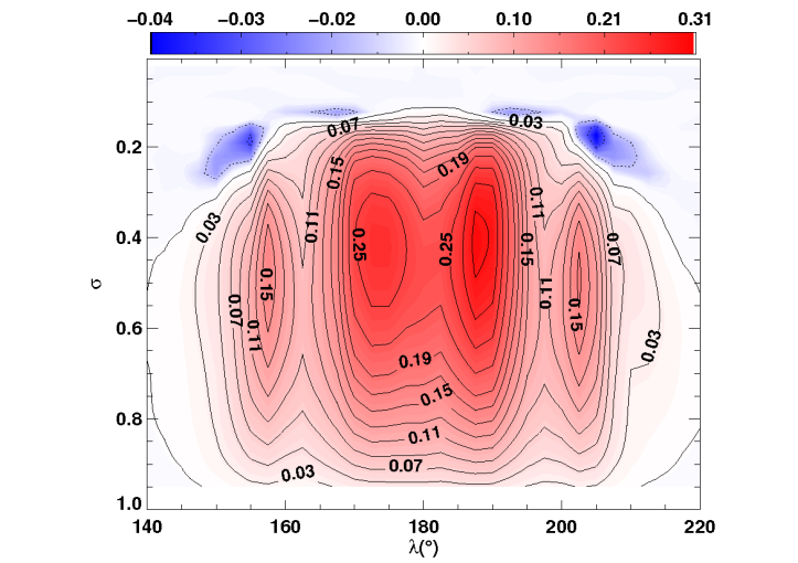
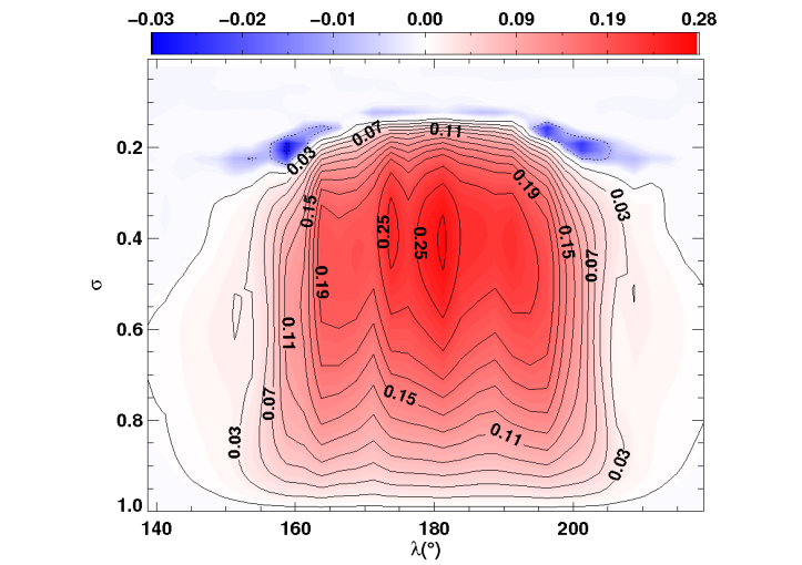
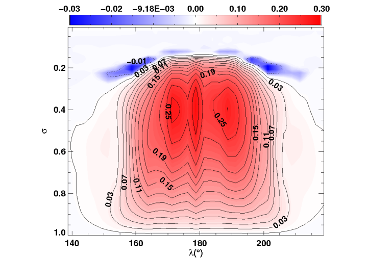
Abbildung 17: Figure showing, for the Tidally Locked Earth test (Merlis and Schneider, 2010; Heng et al., 2011b), the temporally averaged vertical velocities (ms^-1) over the ‘hot spot’ or subsolar point for the ND (top panel), EG_sh (middle panel) and EG (bottom panel) models (see Table 2 for explanation of model types).

Figure 17 shows a broad updraft over the ‘hot spot’ rising to $\sigma\sim 0.2$. The maximum difference in vertical velocity between the EG and EG_sh models are $\sim 0.1$ ms^-1, and these are localised to regions directly above the area of most intense heating, with negligible differences elsewhere. This, as is expected suggests that the simplifications of the dynamical equations are not changing the resulting circulation. The structure of the updraft is marginally different in the ND compared to either of the EG models.

As with the HS and EL test cases we have constructed plots of the difference between the models. We have not produced these plots for the instantaneous results of the temperature field, as differences in such ‘snapshots’ can be dominated by intrinsic temporal variability. Additionally, as with the HS and EL test cases, the differences between the ENDGame model results are an order of magnitude smaller than those found between the ENDGame models and ND, therefore only EG$-$ND is presented. Figures 18 shows the difference, EG$-$ND, of the temporally averaged zonal and meridional wind, as the left and right panels respectively, at the surfaces presented in Figures 14 and 16.

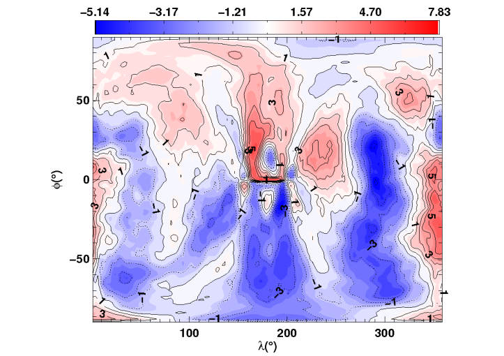
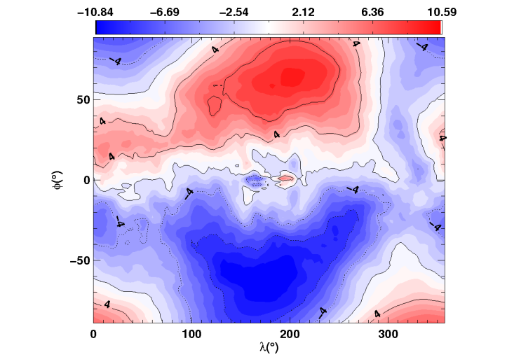
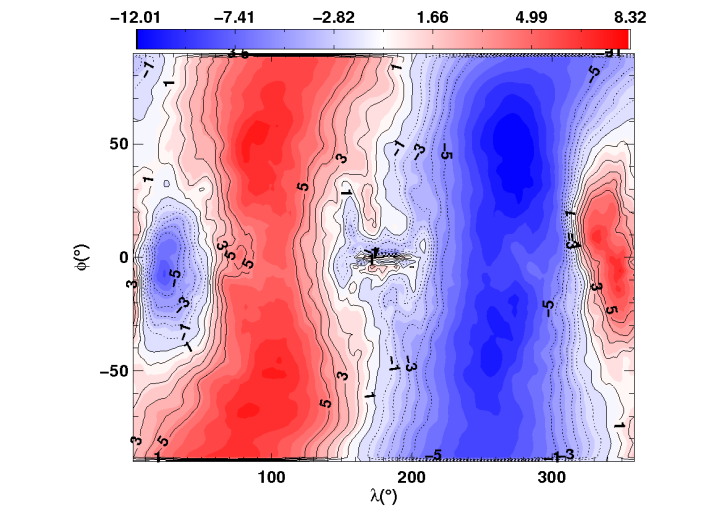
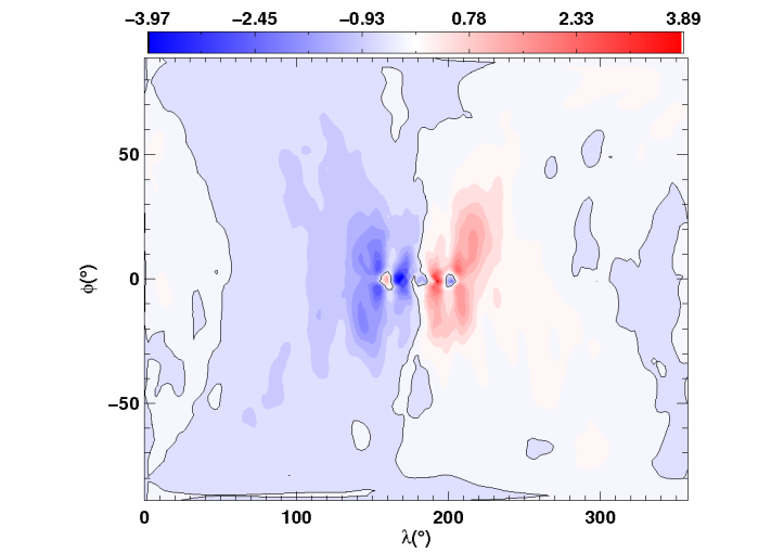
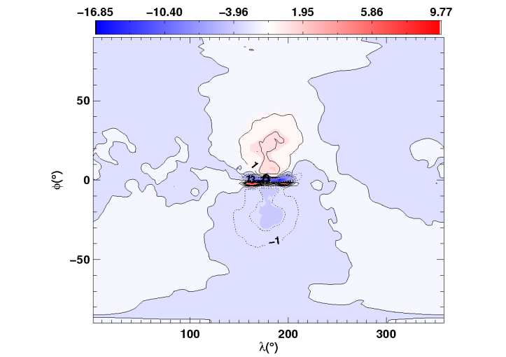
Abbildung 18: Figure, Tidally Locked Earth test (Merlis and Schneider, 2010; Heng et al., 2011b), showing the differences EG$-$ND of the temporally averaged, zonal (left panels) and meridional (right panels) winds (ms^-1), at $\sigma=0.975$, $0.525$, and $0.225$, as the top, middle and bottom rows, respectively (see Table 2 for explanation of model types).

Figure 18 shows the zonal wind at $\sigma=0.225$ is faster in the EG model, over the ND model, as the residual of EG$-$ND is positive, for the positive flow where $\lambda>180^{\circ}$, and negative for the negative flow where $\lambda<180^{\circ}$. Essentially, the zonal flow (left panels) away from the ‘hot spot’ near the upper boundary is faster in the EG model. The opposite is true for the $\sigma=0.975$ surface, where the flow appears to be slowed in the EG, compared to the ND model. The most intriguing difference is found at the $\sigma=0.525$ isobaric–surface where, as shown in Figure 14 the flow structure has inverted about the equator. The meridional flow is also enhanced near the upper boundary, $\sigma=0.225$, and slowed near the surface, in the EG model compared to the ND model (right panels of Figure 18). At the $\sigma=0.525$ surface a systematic change either side of the equator is found, indicative of a reversal of the flow structure one can see in the middle row of Figure 16. For $\lambda>180^{\circ}$ the flow is directed towards the south pole, opposite to that found in ND, and the flow is also reversed for $\lambda<180^{\circ}$. This reversal of flow and difference in the diagnostic plots occurs for all ENDGame models. The flow structure at $\sigma=0.525$ in our ENDGame models match, more closely that found in the spectral code models of Heng et al. (2011b). Whereas the flow for the ND model matches, more closely that found in the finite difference model of Heng et al. (2011b). An explicit polar filter is used in both the ND and the Heng et al. (2011b) finite difference models, but is not required in either ENDGame or the Heng et al. (2011b) spectral model. However, we have run the TLE case using ENDGame but applying a polar filter (as used in the ND model) and found our results still matched, more closely the Heng et al. (2011b) spectral model. This suggests that the difference is due to improvements in the numerical scheme of ENDGame over ND and not the polar filtering scheme.

The structure of the ‘hot spot’ in the top panel of Figure 14 shows the central contour is more elliptical for all the ENDGame solutions, matching more closely (than the ND models) the shape in Figure 13. The structure of the ‘hot spot’ also seems ‘noisier’ in the ENDGame models. The noise exhibited in the ENDGame models is indicative of the reduced implicit damping in the numerical scheme. This can be shown by making the ENDGame scheme more implicit, and therefore, dissipative, by adjusting the temporal weighting coefficient, $\alpha$. Increasing $\alpha$ leads to greater weight being applied to the $i+1$ state and therefore a more implicit scheme. For our ND model and all ENDGame models the $\alpha$ values are $0.7$ and $0.55$ respectively (i.e. ENDGame is more explicit, yet is able to run stably with the same length timestep due to the changes outlined in Section 1.2 and detailed in Wood et al., 2013). Figure 19 shows the temperature structure shown in Figure 14 (top panel) for both the EG using the standard $\alpha=0.55$ (already displayed in Figure 14, rightmost panel, reproduced to aid comparison) and an EG model where $\alpha$ has been increased to 1.0. The fully implicit model presents a smoother temperature structure.

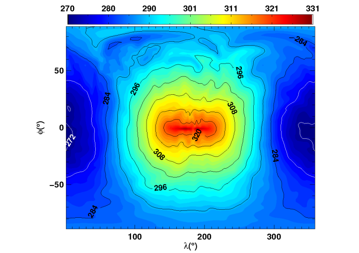
Abbildung 19: Figure showing, for the Tidally Locked Earth test (Merlis and Schneider, 2010; Heng et al., 2011b), showing temperature at 1200 days and $\sigma=0.975$, for the EG models (see Table 2 for explanation of model types) using $\alpha$ of $0.55$ and $1.0$ (top and bottom panels, respectively).

To attempt to isolate differences caused only by the numerical scheme we compare the nature of the meridional circulation for the TLE models using ND and EG_gc, since the ND and EG_gc models solve identical equations sets. Figure 20 shows the temporally and meridionally averaged meridional flow for the ND and EG_gc models. The average is performed in a point–wise fashion, i.e. $\int\,vd\,\phi$ as opposed to $\int\,\cos\phi vd\,\phi$, to emphasise differences in flow over the pole. In a non–rotating system, where the Coriolis force is zero, one would expect a symmetric meridional flow, so the latitudinal average should be close to zero. For the TLE case the rotation is slow, with a Rossby number of, $R_{o}=\frac{U}{Lf}\sim\frac{30}{4\times 10^{7}\times 2\times 2\times 10^{-7}}\sim 2.0$ (where $U$ is the horizontal velocity scale, $L$ the length scale and $f=2\Omega\sin\phi$; the Coriolis frequency or parameter), indicating negligible effects of rotation.

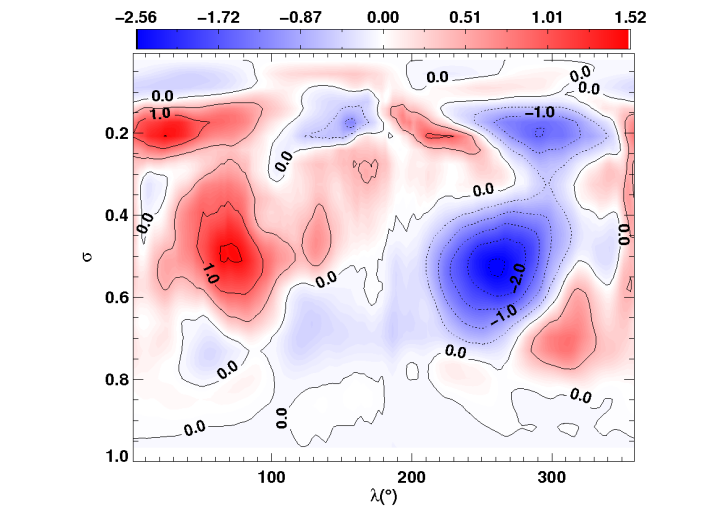
Abbildung 20: Figure showing, for the Tidally Locked Earth test (Merlis and Schneider, 2010; Heng et al., 2011b), the temporally and meridionally averaged meridional flow for the ND (top panel) and EG_gc (bottom panel) models (see Table 2 for explanation of model types).

Figure 20 shows that the meridional average is almost an order of magnitude larger in the ND case, compared with the EG_gc model. To further examine the symmetry of meridional circulation cells, we define a stream function ($\Psi$) as

$$\Psi=-2\pi\cos\phi\int_{R_{\rm p}}^{r}r\bar{v}(\phi,\tilde{r})d\tilde{r},\\$$ (21)

where $\bar{v}$ denotes the zonally averaged meridional velocity.

Figure 21 shows this diagnostic as a function of latitude and height for the ND and EG_gc models. The values assigned to the contours in both panels of Figure 21 are the same. The results are similar for both models but the circulation cells are marignally more symmetric (especially closer to the surface) for the EG_gc models. The lower (in altitude) circulation cells are direct i.e. caused by the heating of the atmosphere, whilst the higher cells are indirect. As shown in Heng et al. (2011a) the circulation cells differ on the day and night side. However, here we do not split by hemisphere as we are simply interested in the comparison between models.

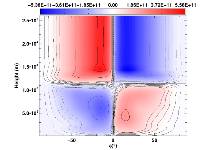
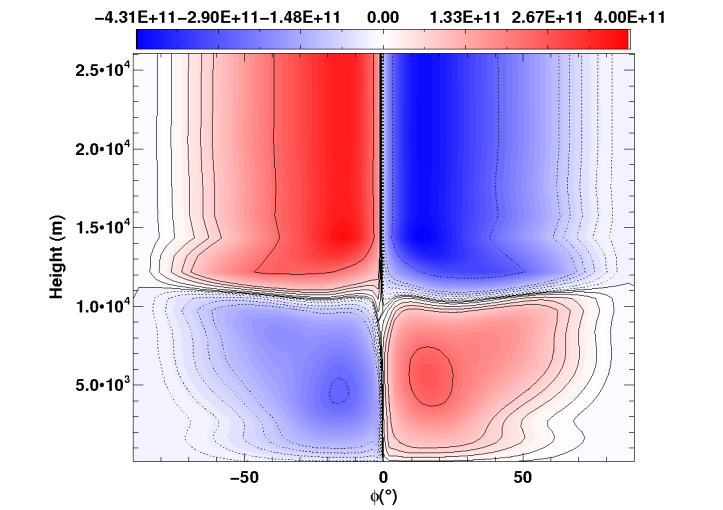
Abbildung 21: Figure showing, for the Tidally Locked Earth test (Merlis and Schneider, 2010; Heng et al., 2011b), the streamfunction $\Psi$ (defined in text, see Equation 21) for the ND (top panel) and EG_gc (right panel) models (see Table 2 for explanation of model types). The contours in both panels are the same and set at values $-5.0\times 10^{11}$, $-2.5\times 10^{11}$, $-1.0\times 10^{11}$, $-7.5\times 10^{10}$, $-5.0\times 10^{10}$, $-2.5\times 10^{10}$, $-1.0\times 10^{10}$, 0.0, $1.0\times 10^{10}$, $2.5\times 10^{10}$, $5.0\times 10^{10}$, $7.5\times 10^{10}$, $1.0\times 10^{11}$, $2.5\times 10^{11}$ and $5.0\times 10^{11}$.

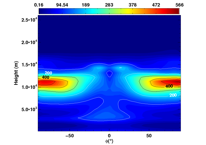
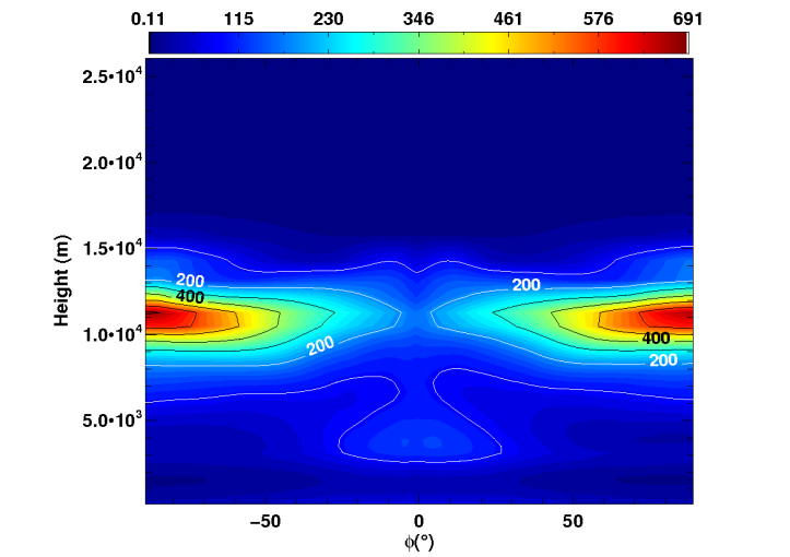
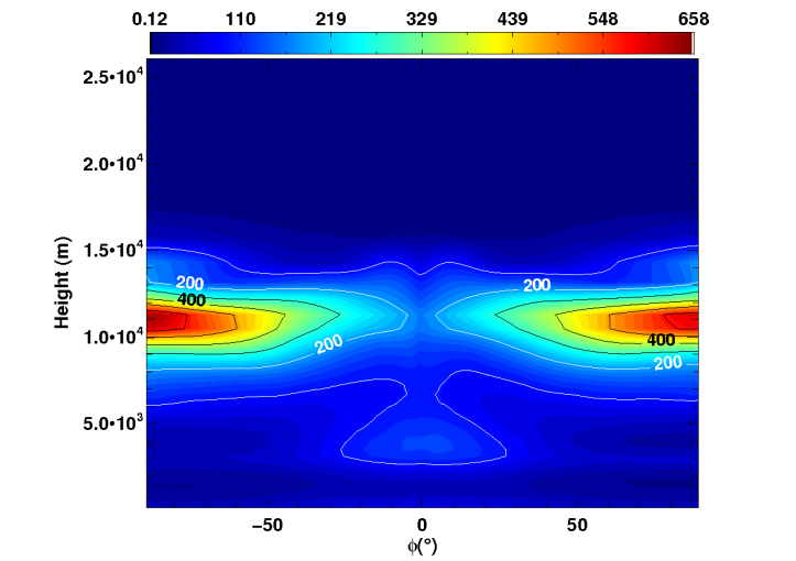
Abbildung 22: Figure, for the Tidally Locked Earth test (Merlis and Schneider, 2010; Heng et al., 2011b), showing the zonally (in geometric height) and temporally averaged Eddy Kinetic Energy (EKE, see Section 2.1) as a function of latitude and height. Top left panel ND, top right panel EG_sh, bottom left panel EG_gc and bottom right panel EG models (see Table 2 for explanation of model types). Note the contours (solid lines) are the same in all plots.

Figure 22 shows the EKE, zonally (along geometric height surfaces) and temporally averaged ($\overline{{\rm EKE}}^{\lambda_{\rm z}t}$), for the ND and all ENDGame models. Figure 22 shows more distinct differences when comparing ND to any of the ENDGame models, compared to the HS or EL test cases. In the TLE case the kinetic energy associated with the eddies clearly increases when moving from ND to ENDGame. Additionally, the structure of the peak activity region, which extends from mid–latitudes over the poles, is flatter (in altitude) in the ENDGame models. One can also observe a move to increased hemispherical symmetry when moving from ND through EG_sh and EG_gc to EG. This shows that ENDGame produces a more spherically symmetric pattern of eddies, closer to what one would expect in a slowly rotating system. Furthermore, it shows that subsequent relaxation of the approximations to the equations of motion slightly improves the symmetry of the solution. Again, as with the EL test cases, we present the difference in the $\overline{{\rm EKE}}^{\lambda_{\rm z},t}$, in the sense EG$-$ND in Figure 23, where the ENDGame model differences are not shown as they are an order of magnitude smaller than those between the EG and ND models.

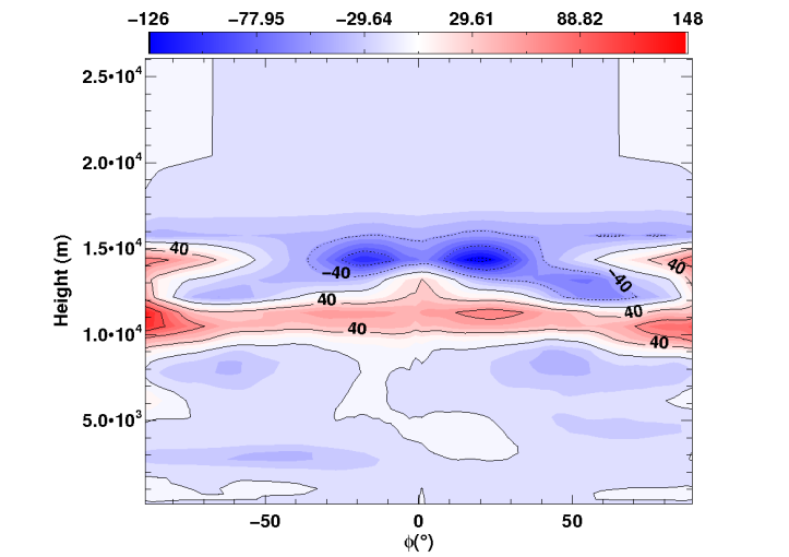
Abbildung 23: Figure, for the Tidally Locked Earth test (Merlis and Schneider, 2010; Heng et al., 2011b), showing the differences EG$-$ND of the zonally and temporally averaged EKE (see Table 2 for explanation of model types).

As with the previous test cases, and evident from the prognostic fields $T$, $u$ and $v$, all the ENDGame models show a remarkable level of consistency in the solution. However, as in the HS and EL test cases, significant differences in the $\overline{{\rm EKE}}^{\lambda_{\rm z},t}$, are found when comparing EG to ND. The magnitude of the peak relative differences in $\overline{{\rm EKE}}^{\lambda_{\rm z}t}$ are $\sim$8.0, 0.40 and 0.61 for the differences EG$-$ND, EG$-$EG_gc and EG$-$EG_sh, respectively. The relative difference for the EG$-$ND is much larger than that found in either the HS or EL test cases. The peak $\overline{{\rm EKE}}^{\lambda_{\rm z},t}$, is larger in the EG model and the peak appears to shift lower in the atmosphere, when compared to the ND model.

Whilst features such as the increased hemispherical symmetry of the flow found in the ENDGame models, are close to what one might physically expect, this test case (and the others) is not a definitive test to demonstrate that the flow is handled better in ENDGame. However, it is clear that they are at least handled differently. The difficulty for tests such as these is that a correct, or analytical answer, for the flow does not exist.

We have demonstrated that both the ND and ENDGame dynamical cores of the Met Office UM produce 3D idealised large–scale and long–term flows consistent both with previous works, and under varying approximations to the full equations of motions. These tests are the Held–Suarez test (Held and Suarez, 1994), an Earth–like test (Heng et al., 2011b; Menou and Rauscher, 2009) and a hypothetical tidally locked Earth (Merlis and Schneider, 2010; Heng et al., 2011b). Qualitative agreement was found for the results of these three idealised test cases, both between the UM dynamical cores and when compared with literature results. Furthermore, the consistency of the solutions was not changed when invoking the approximations possible in the ENDGame equation set, all of which should be applicable for our test cases, namely, the ‘shallow–atmosphere’ approximation, as a whole, or just the assumption of constant gravity. We also found tentative evidence of differences in the circulation, for the TLE case, between the ENDGame and ND cores probably caused by changes in the temporal and spatial discretisation.

These results should be viewed as complementary to more analytical testing. For our project, namely adapting the UM with a state–of–the–art dynamical core to exoplanets, this work is a crucial first step in confirming the consistency of the code, both with other GCMs and, under different approximations to the full equations of motion. We have also tested the code in flow regimes with features in common with the subset of exoplanets termed hot Jupiters (which our project aims to characterise), i.e. a hypothetical tidally locked earth. For the flow regimes of hot Jupiters the solutions to the equations of motion are expected to differ under the different approximations featured in this work. Furthermore, these objects are severely observationally under–constrained, so rigorous testing is required. We will present the next step of this project, involving adaptation of the code and simplified giant planet test cases in a future work (Mayne et al, submitted).

Anhang A

Appendix

A.1 A note on comparison with the work of Heng et al. (2011b).

Heng et al. (2011b) perform both finite–difference and spectral models of the test cases using the same GCM (the Princeton Flexible Modeling System, FMS). In this work we concentrate our comparison with the results of the finite–difference versions of the test, as the UM also adopts a finite–difference method. Additionally, it is not clear which $\sigma$ surface Heng et al. (2011b) select when producing plots of the atmosphere as a function of latitude and longitude, in the spectral case. The spectral version of the FMS dynamical core performs vertical finite–differencing using a Simmons-Burridge scheme. Heng et al. (2011b) state, the prognostic variable output is not exactly at the mid–point of the vertical half–levels, and when presenting results they usually quote the $\sigma$ of the bottom pair of half–levels. Therefore, some uncertainty exists over which $\sigma$ surface the resulting plots are produced from. For the finite–difference results Heng et al. (2011b) state that the labeling of the model layers adopts the same system as the spectral version, i.e. each layer is actually labeled with the value of the larger $\sigma$ half–level. This may result in a slight translation, or vertical shift, when we present plots with $\sigma$ as the vertical axis. As comparison of our results and those of Heng et al. (2011b) show, in Section 2.4 this effect is negligible. However, for horizontal slices at a prescribed $\sigma$ this will result in the flow being presented at a different pressure surface. In effect, therefore, we assume that if a figure from Heng et al. (2011b) is presented as representative of the flow at a given $\sigma$, that actually the flow is that present at $\sigma-1.0/(2\times 20)$ (i.e. $\sigma-0.025$), as Heng et al. (2011b) use 20 uniformly distributed vertical levels (with associated half–levels) spaced evenly in $\sigma$. Therefore, our Figures will be presented using the actual $\sigma$ value of the model, where we have interpolated our prognostic variables onto this $\sigma$ surface.

A.2 Vertical Level Placements

Table A.2 shows the positions of the vertical ($\theta$), levels in non–dimensional height units ($\eta$), alongside the size of the domain $H$ and the approximate $\sigma$ value (see Section 2.1 for explanation).

Tabelle 4: Table showing the dimensionless vertical coordinate for the $\theta$ levels of the three model setups, $\eta_{\theta}$ ($\eta=z/H$) alongside the approximate $\sigma$ levels and the model domain height ($H$).

Test case:		Held-Suarez (HS)	Earth-Like (EL)	Tidally Locked Earth (TLE)
$H$ (m)		30975.0	30964.0	30056.0
Level	$\sim$$\sigma$	$\eta_{\theta}$
0	1.00	0.000000	0.000000	0.000000
1	0.97	0.009072	0.004521	0.009915
2	0.94	0.018111	0.009010	0.019763
3	0.91	0.027506	0.026967	0.029977
4	0.88	0.036901	0.036203	0.040192
5	0.84	0.046295	0.045408	0.050472
6	0.81	0.056433	0.055290	0.061951
7	0.78	0.066764	0.065495	0.073463
8	0.75	0.077094	0.075701	0.085108
9	0.72	0.088103	0.086423	0.097651
10	0.69	0.099467	0.097694	0.110194
11	0.66	0.110896	0.109030	0.123303
12	0.63	0.123099	0.121011	0.137011
13	0.60	0.135626	0.133510	0.150852
14	0.57	0.148539	0.146331	0.165824
15	0.53	0.162260	0.159928	0.180829
16	0.50	0.176303	0.174009	0.197065
17	0.47	0.191251	0.188897	0.213501
18	0.44	0.206780	0.204560	0.231302
19	0.41	0.223245	0.221128	0.249468
20	0.38	0.240613	0.238826	0.269331
21	0.35	0.259112	0.257654	0.289959
22	0.32	0.278935	0.278000	0.312018
23	0.28	0.300371	0.300026	0.336039
24	0.26	0.323584	0.324021	0.361791
25	0.22	0.349379	0.350698	0.389839
26	0.19	0.378563	0.380668	0.421047
27	0.16	0.412365	0.415321	0.456614
28	0.13	0.453010	0.457338	0.498336
29	0.10	0.504310	0.510690	0.549607
30	0.07	0.574851	0.583419	0.621540
31	0.04	0.687780	0.698908	0.736126
32	0.01	1.000000	1.000000	1.000000