An optimal three-way stable and monotonic spectrum of bounds on quantiles:
a spectrum of coherent measures of financial risk and economic inequality

Abstract

A certain spectrum $\big{(}P_{\alpha}(X;x)\big{)}_{\alpha\in[0,\infty]}$ of upper bounds on the tail probability $\operatorname{\mathsf{P}}(X\geqslant x)$, with $P_{0}(X;x)=\operatorname{\mathsf{P}}(X\geqslant x)$ and $P_{\infty}(X;x)$ being the best possible exponential upper bound on $\operatorname{\mathsf{P}}(X\geqslant x)$, is shown to be stable and monotonic in $\alpha$, $x$, and $X$, where $x$ is a real number and $X$ is a random variable. The bounds $P_{\alpha}(X;x)$ are optimal values in certain minimization problems. The corresponding spectrum $\big{(}Q_{\alpha}(X;p)\big{)}_{\alpha\in[0,\infty]}$ of upper bounds on the $(1-p)$-quantile of $X$ is shown as well to be stable and monotonic in $\alpha$, $p$, and $X$, with $Q_{0}(X;p)$ equal the largest $(1-p)$-quantile of $X$. In fact, $P_{\alpha}(X;x)$ and $Q_{\alpha}(X;p)$ are nondecreasing in $X$ with respect to the stochastic dominance of any order $\gamma\in[1,\alpha+1]$. It is shown that for small enough values of $p$ the quantile bounds $Q_{\alpha}(X;p)$ are close enough to the true quantiles $Q_{0}(X;p)$ provided that the right tail of the distribution of $X$ is light enough and regular enough, depending on $\alpha$. Moreover, it is shown that the quantile bounds $Q_{\alpha}(X;p)$ possess the crucial property of the subadditivity in $X$ if $\alpha\in[1,\infty]$, as well as the positive homogeneity and translation invariance properties, and thus constitute a continuous spectrum of so-called coherent measures of risk. A number of other useful properties of the bounds $P_{\alpha}(X;x)$ and $Q_{\alpha}(X;p)$ are established. In particular, it is shown that, quite similarly to the bounds $P_{\alpha}(X;x)$ on the tail probabilities, the quantile bounds $Q_{\alpha}(X;p)$ are the optimal values in certain minimization problems. This allows for a comparatively easy incorporation of the bounds $P_{\alpha}(X;x)$ and $Q_{\alpha}(X;p)$ into more specialized optimization problems, with additional restrictions, say on the distribution of the random variable $X$. It is shown that the mentioned minimization problems for which $P_{\alpha}(X;x)$ and $Q_{\alpha}(X;p)$ are the optimal values are in a certain sense dual to each other; in the special case $\alpha=\infty$ this corresponds to the bilinear Legendre–Fenchel duality. In finance, the $(1-p)$-quantile $Q_{0}(X;p)$ is known as the value-at-risk (VaR), whereas the value of $Q_{1}(X;p)$ is known as the conditional value-at-risk (CVaR) and also as the expected shortfall (ES), average value-at-risk (AVaR), and expected tail loss (ETL). Also in the present paper, a short proof of the well-known Rockafellar–Uryasev–Pflug theorem that VaR is a minimizer in the Rockafellar–Uryasev variational representation of CVaR is provided. More generally, the minimizers in the variational representation of $Q_{\alpha}(X;p)$ are described in detail for any $\alpha\in[1,\infty)$. A generalization of the Cillo–Delquie necessary and sufficient condition for the so-called mean-risk (M-R) to be nondecreasing with respect to the stochastic dominance of order $1$ is presented, with a short proof. Moreover, a necessary and sufficient condition for the M-R measure to be coherent is given. It is shown that the quantile bounds $Q_{\alpha}(X;p)$ can be used as measures of economic inequality. The spectrum parameter $\alpha$ may be considered an index of sensitivity: the greater is the value of $\alpha$, the greater is the sensitivity of the function $Q_{\alpha}(\cdot;p)$ to risk/inequality. The problems of effective computation of $P_{\alpha}(X;x)$ and $Q_{\alpha}(X;p)$ are considered.

Bounds on quantiles

Iosif Pinelis

Department of Mathematical Sciences
Michigan Technological University
Houghton, Michigan 49931, USA
E-mail: [ipinelis@mtu.edu]e1

keywordAMSAMS 2010 subject classifications:

[class=AMS] [Primary ]52A41 60E15 26A51 26B25 91B30 91B82 [; secondary ]60E15 90C25 90C26 49J45 49J55 49K30 49K40 39B62

probability inequalities extremal problems tail probabilities quantiles coherent measures of risk measures of economic inequality value-at-risk (VaR) conditional value-at-risk (CVaR) expected shortfall (ES) average value-at-risk (AVaR) expected tail loss (ETL) mean-risk (M-R) Gini’s mean difference stochastic dominance stochastic orders

chapter

subsubsection

1 An optimal three-way stable and three-way monotonic spectrum of upper bounds on tail probabilities

Consider the family $(h_{\alpha})_{\alpha\in[0,\infty]}$ of functions $h_{\alpha}\colon\mathbb{R}\to\mathbb{R}$ given by the formula

$$h_{\alpha}(u):=\left\{\begin{aligned} &\,\mathsf{I}\{u\geqslant 0\}&&\text{\ \ if }\alpha=0,\\ &(1+u/\alpha)_{+}^{\alpha}&&\text{\ \ if }0<\alpha<\infty,\\ &e^{u}&&\text{\ \ if }\alpha=\infty\end{aligned}\right.$$ (1.1)

for all $u\in\mathbb{R}$. Here, as usual, $\,\mathsf{I}\{\cdot\}$ denotes the indicator function, $u_{+}:=0\vee u$ and $u_{+}^{\alpha}:=(u_{+})^{\alpha}$ for all real $u$.

Obviously, the function $h_{\alpha}$ is nonnegative and nondecreasing for each $\alpha\in[0,\infty]$, and it is also continuous for each $\alpha\in(0,\infty]$. Moreover, it is easy to see that, for each $u\in\mathbb{R}$,

$$h_{\alpha}(u)\text{ is nondecreasing and continuous in }\alpha\in[0,\infty].$$ (1.2)

Next, let us use the functions $h_{\alpha}$ as generalized moment functions and thus introduce the generalized moments

$$A_{\alpha}(X;x)(\lambda):=\operatorname{\mathsf{E}}h_{\alpha}\big{(}\lambda(X-x)\big{)}.$$ (1.3)

Here and in what follows, unless otherwise specified, $X$ is any random variable (r.v.), $x\in\mathbb{R}$, $\alpha\in[0,\infty]$, and $\lambda\in(0,\infty)$. Since $h_{\alpha}\geqslant 0$, the expectation in (1.3) is always defined, but may take the value $\infty$. It may be noted that in the particular case $\alpha=0$ one has

$$A_{0}(X;x)(\lambda)=\operatorname{\mathsf{P}}(X\geqslant x),$$ (1.4)

which does not actually depend on $\lambda\in(0,\infty)$.

Now one can introduce the expressions

$$P_{\alpha}(X;x):=\inf_{\lambda\in(0,\infty)}A_{\alpha}(X;x)(\lambda)=\left\{\begin{aligned} &\operatorname{\mathsf{P}}(X\geqslant x)&&\text{\ \ if }\alpha=0,\\ &\inf_{\lambda\in(0,\infty)}\operatorname{\mathsf{E}}\big{(}1+\lambda(X-x)/\alpha)_{+}^{\alpha}&&\text{\ \ if }0<\alpha<\infty,\\ &\inf_{\lambda\in(0,\infty)}\operatorname{\mathsf{E}}e^{\lambda(X-x)}&&\text{\ \ if }\alpha=\infty.\end{aligned}\right.$$ (1.5)

By (1.2), $A_{\alpha}(X;x)(\lambda)$ and $P_{\alpha}(X;x)$ are nondecreasing in $\alpha\in[0,\infty]$. In particular,

$$P_{0}(X;x)=\operatorname{\mathsf{P}}(X\geqslant x)\leqslant P_{\alpha}(X;x).$$ (1.6)

It will be shown later (see Proposition 1.4) that $P_{\alpha}(X;x)$ also largely inherits the property of $h_{\alpha}(u)$ of being continuous in $\alpha\in[0,\infty]$.

The definition (1.5) can be rewritten as

$$P_{\alpha}(X;x)=\inf_{t\in T_{\alpha}}{\tilde{A}}_{\alpha}(X;x)(t),$$ (1.7)

where

$$T_{\alpha} :=\left\{\begin{aligned} &\mathbb{R}&&\text{\ \ if $\alpha\in[0,\infty)$,}\\ &(0,\infty)&&\text{\ \ if $\alpha=\infty$}\end{aligned}\right.$$ (1.8)

and

$${\tilde{A}}_{\alpha}(X;x)(t) :=\left\{\begin{aligned} &\frac{\operatorname{\mathsf{E}}(X-t)_{+}^{\alpha}}{(x-t)_{+}^{\alpha}}&&\text{ if }\alpha\in[0,\infty),\\ &\operatorname{\mathsf{E}}e^{(X-x)/t}&&\text{ if }\alpha=\infty;\end{aligned}\right.$$ (1.9)

here and subsequently, we also use the conventions $0^{0}:=0$ and $\frac{a}{0}:=\infty$ for all $a\in[0,\infty]$. The alternative representation (1.7) of $P_{\alpha}(X;x)$ follows because (i) $A_{\alpha}(X;x)(\lambda)={\tilde{A}}_{\alpha}(X;x)(x-\alpha/\lambda)$ for $\alpha\in(0,\infty)$, (ii) $A_{\infty}(X;x)(\lambda)={\tilde{A}}_{\infty}(X;x)(1/\lambda)$, and (iii) $P_{0}(X;x)=\operatorname{\mathsf{P}}(X\geqslant x)=\inf_{t\in(-\infty,x)}\operatorname{\mathsf{P}}(X>t)=\inf_{t\in(-\infty,x)}{\tilde{A}}_{0}(X;x)(t)$.

In view of (1.7), one can see (cf. [38, Corollary 2.3]) that, for each $\alpha\in[0,\infty]$, $P_{\alpha}(X;x)$ is the optimal (that is, least possible) upper bound on the tail probability $\operatorname{\mathsf{P}}(X\geqslant x)$ given the generalized moments $\operatorname{\mathsf{E}}g_{\alpha;t}(X)$ for all $t\in T_{\alpha}$, where

$$g_{\alpha;t}(u):=\left\{\begin{aligned} &(u-t)_{+}^{\alpha}&&\text{ if }\alpha\in[0,\infty),\\ &e^{u/t}&&\text{ if }\alpha=\infty.\end{aligned}\right.$$ (1.10)

In fact (cf. e.g. [43, Proposition 3.3]), the bound $P_{\alpha}(X;x)$ remains optimal given the larger class of generalized moments $\operatorname{\mathsf{E}}g(X)$ for all functions $g\in\mathscr{H}^{\alpha}$, where

$$\mathscr{H}^{\alpha}:=\big{\{}g\in\mathbb{R}^{\mathbb{R}}\colon g(u)=\textstyle{\int\nolimits_{\mathbb{R}}}g_{\alpha;t}(u)\,\mu(dt)\text{ for some $\mu\in{\mathrm{M}}_{\alpha}$ and all $u\in\mathbb{R}$}\big{\}},$$ (1.11)

${\mathrm{M}}_{\alpha}$ denotes the set of all nonnegative Borel measures on $T_{\alpha}$, and, as usual, $\mathbb{R}^{\mathbb{R}}$ stands for the set of all real-valued functions on $\mathbb{R}$. By [39, Proposition 1(ii)] and [43, Proposition 3.4],

$$0\leqslant\alpha<\beta\leqslant\infty\quad\text{implies}\quad\mathscr{H}^{\alpha}\supseteq\mathscr{H}^{\beta}.$$ (1.12)

This provides the other way to come to the mentioned conclusion that

$$P_{\alpha}(X;x)\text{ is nondecreasing in }\alpha\in[0,\infty].$$ (1.13)

By [40, Proposition 1.1], the class $\mathscr{H}^{\alpha}$ of generalized moment functions can be characterized as follows in the case when $\alpha$ is a natural number: for any $g\in\mathbb{R}^{\mathbb{R}}$, one has $g\in\mathscr{H}^{\alpha}$ if and only if $g$ has finite derivatives $g^{(0)}:=g,g^{(1)}:=g^{\prime},\dots,g^{(\alpha-1)}$ on $\mathbb{R}$ such that $g^{(\alpha-1)}$ is convex on $\mathbb{R}$ and $\lim_{x\to-\infty}g^{(j)}(x)=0$ for $j=0,1,\dots,\alpha-1$. Also, by [43, Proposition 3.4], $g\in\mathscr{H}^{\infty}$ if and only if $g$ is infinitely differentiable on $\mathbb{R}$, and $g^{(j)}\geqslant 0$ on $\mathbb{R}$ and $\lim_{x\to-\infty}g^{(j)}(x)=0$ for all $j=0,1,\dots$.

Thus, the greater the value of $\alpha$, the narrower and easier to deal with is the class $\mathscr{H}^{\alpha}$ and the smoother are the functions comprising $\mathscr{H}^{\alpha}$. However, the greater the value of $\alpha$, the farther away is the bound $P_{\alpha}(X;x)$ from the true tail probability $\operatorname{\mathsf{P}}(X\geqslant x)$.

Of the bounds $P_{\alpha}(X;x)$, the loosest and easiest one to get is $P_{\infty}(X;x)$, the so-called exponential upper bound on the tail probability $\operatorname{\mathsf{P}}(X\geqslant x)$. It is used very widely, in particular when $X$ is the sum of independent r.v.’s $X_{i}$, in which case one can rely on the factorization $A_{\alpha}(X;x)(\lambda)=e^{-\lambda x}\prod_{i}\operatorname{\mathsf{E}}e^{\lambda X_{i}}$. A bound very similar to $P_{3}(X;x)$ was introduced in [16] in the case when $X$ the sum of independent bounded r.v.’s; see also [36, 15, 37]. For any $\alpha\in(0,\infty)$, the bound $P_{\alpha}(X;x)$ is a special case of a more general bound given in [38, Corollary 2.3]; see also [38, Theorem 2.5]. For some of the further developments in this direction see [39, 7, 8, 41, 42, 9, 43]. The papers mentioned in this paragraph used the representation (1.7) of $P_{\alpha}(X;x)$, rather than the new representation (1.5). The new representation appears, not only of more unifying form, but also more convenient as far as such properties of $P_{\alpha}(X;x)$ as the monotonicity in $\alpha$ and the continuity in $\alpha$ and in $X$ are concerned; cf. (1.2) and the proofs of Propositions 1.4 and 1.5; those proofs, as well as proofs of most of the other statements in this paper, are given in Appendix A. Yet another advantage of the representation (1.5) is that, for $\alpha\in[1,\infty)$, the function $A_{\alpha}(X;x)(\cdot)$ inherits the convexity property of $h_{\alpha}$, which facilitates the minimization of $A_{\alpha}(X;x)(\lambda)$ in $\lambda$, as needed to find $P_{\alpha}(X;x)$ by (1.5); relevant details on the remaining “difficult case” $\alpha\in(0,1)$ can be found in Section 3.1.

On the other hand, the “old” representation (1.7) of $P_{\alpha}(X;x)$ is more instrumental in establishing the mentioned connection with the classes $\mathscr{H}^{\alpha}$ of generalized moment functions; in proving part (iii) of Proposition 1.2; and in discovering and proving Theorem 2.3.

***

Some of the more elementary properties of $P_{\alpha}(X;x)$ are presented in

Proposition 1.1.

1. $P_{\alpha}(X;x)$ is nonincreasing in $x\in\mathbb{R}$.

2. If $\alpha\in(0,\infty)$ and $\operatorname{\mathsf{E}}X_{+}^{\alpha}=\infty$, then $P_{\alpha}(X;x)=\infty$ for all $x\in\mathbb{R}$.

3. If $\alpha=\infty$ and $\operatorname{\mathsf{E}}e^{\lambda X}=\infty$ for all real $\lambda>0$, then $P_{\infty}(X;x)=\infty$ for all $x\in\mathbb{R}$.

4. If $\alpha\in(0,\infty)$ and $\operatorname{\mathsf{E}}X_{+}^{\alpha}<\infty$, then $P_{\alpha}(X;x)\to 1$ as $x\to-\infty$ and $P_{\alpha}(X;x)\to 0$ as $x\to\infty$, so that $0\leqslant P_{\alpha}(X;x)\leqslant 1$ for all $x\in\mathbb{R}$.

5. If $\alpha=\infty$ and $\operatorname{\mathsf{E}}e^{\lambda_{0}X}<\infty$ for some real $\lambda_{0}>0$, then $P_{\alpha}(X;x)\to 1$ as $x\to-\infty$ and $P_{\alpha}(X;x)\to 0$ as $x\to\infty$, so that $0\leqslant P_{\alpha}(X;x)\leqslant 1$ for all $x\in\mathbb{R}$.

In view of Proposition 1.1, it will be henceforth assumed by default that the tail bounds $P_{\alpha}(X;x)$ – as well as the quantile bounds $Q_{\alpha}(X;p)$, to be introduced in Section 2, and also the corresponding expressions $A_{\alpha}(X;x)(\lambda)$, ${\tilde{A}}_{\alpha}(X;x)(t)$, $B_{\alpha}(X;p)(t)$, and ${}_{\alpha-1}Q(X;p)$ as in (1.3), (1.9), (2.9), and (3.15) – are defined and considered only for r.v.’s $X\in\mathscr{X}_{\alpha}$ (unless indicated otherwise), where

$$\mathscr{X}_{\alpha}:=\left\{\begin{aligned} &\mathscr{X}&&\text{\ \ if }\alpha=0,\\ &\big{\{}X\in\mathscr{X}\colon\operatorname{\mathsf{E}}X_{+}^{\alpha}<\infty\big{\}}&&\text{\ \ if }\alpha\in(0,\infty),\\ &\big{\{}X\in\mathscr{X}\colon\Lambda_{X}\neq\emptyset\big{\}}&&\text{\ \ if }\alpha=\infty,\end{aligned}\right.$$

$\mathscr{X}$ is the set of all real-valued r.v.’s on a given probability space (implicit in this paper), and

$$\Lambda_{X}:=\big{\{}\lambda\in(0,\infty)\colon\operatorname{\mathsf{E}}e^{\lambda X}<\infty\big{\}}.$$ (1.14)

Observe that the set $\mathscr{X}_{\alpha}$ is a convex cone: for any $\theta\in[0,\infty)$ and any $X$ and $Y$ in $\mathscr{X}_{\alpha}$, the r.v.’s $\theta X$ and $X+Y$ are in $\mathscr{X}_{\alpha}$. Indeed, the conclusion that $\theta X\in\mathscr{X}_{\alpha}$ for any $\theta\in[0,\infty)$ and $X\in\mathscr{X}_{\alpha}$ is obvious. Concerning the conclusion that $X+Y\in\mathscr{X}_{\alpha}$ for any $X$ and $Y$ in $\mathscr{X}_{\alpha}$, use the inequalities $\operatorname{\mathsf{E}}(X+Y)_{+}^{\alpha}\leqslant\operatorname{\mathsf{E}}(X_{+}+Y_{+})^{\alpha}\leqslant\operatorname{\mathsf{E}}X_{+}^{\alpha}+\operatorname{\mathsf{E}}Y_{+}^{\alpha}$ if $\alpha\in(0,1]$, Minkowski’s inequality $\|X_{+}+Y_{+}\|_{\alpha}\leqslant\|X_{+}\|_{\alpha}+\|Y_{+}\|_{\alpha}$ if $\alpha\in[1,\infty)$, and Hölder’s inequality $\operatorname{\mathsf{E}}e^{\lambda(X+Y)}\leqslant\big{(}\operatorname{\mathsf{E}}e^{p\lambda X}\big{)}^{1/p}\big{(}\operatorname{\mathsf{E}}e^{q\lambda X}\big{)}^{1/q}$ for any positive $p$ and $q$ such that $\frac{1}{p}+\frac{1}{q}=1$. Here, as usual, $\|Z\|_{\alpha}:=(\operatorname{\mathsf{E}}|Z|^{\alpha})^{1/\alpha}$, the $\mathscr{L}^{\alpha}$-norm of a r.v. $Z$ – which is actually a norm if and only if $\alpha\geqslant 1$. Also, it is obvious that the cone $\mathscr{X}_{\alpha}$ contains all real constants.

It follows from Proposition 1.1 and (1.6) that

$$P_{\alpha}(X;x) x\in\mathbb{R} P_{\alpha}(X;(-\infty)+)=1 P_{\alpha}(X;\infty-)=0$$ is nonincreasing in , with and . (1.15)

Here, as usual, $f(a+)$ an $f(a-)$ denote the right and left limits of $f$ at $a$.

One can say more in this respect. To do that, introduce

$$x_{*}:=x_{*,X}:=\sup\operatorname{supp}X\quad\text{and}\quad p_{*}:=p_{*,X}:=\operatorname{\mathsf{P}}(X=x_{*}).$$ (1.16)

Here, as usual, $\operatorname{supp}X$ denotes the support set of (the distribution of the r.v.) $X$; speaking somewhat loosely, $x_{*}$ is the maximum value taken by the r.v. $X$, and $p_{*}$ is the probability with which this value is taken. It is of course possible that $x_{*}=\infty$, in which case necessarily $p_{*}=0$, since the r.v. $X$ was assumed to be real-valued.

Introduce also

$$x_{\alpha}:=x_{\alpha,X}:=\inf E_{\alpha}(1),$$ (1.17)

where

$$E_{\alpha}(p):=E_{\alpha,X}(p):=\{x\in\mathbb{R}\colon P_{\alpha}(X;x)<p\}.$$ (1.18)

Recall that, according to the standard convention, for any subset $E$ of $\mathbb{R}$, $\inf E=\infty$ if and only if $E=\emptyset$.

Now one can state

Proposition 1.2.

1. For all $x\in[x_{*},\infty)$ one has $P_{\alpha}(X;x)=P_{0}(X;x)=\operatorname{\mathsf{P}}(X\geqslant x)=\operatorname{\mathsf{P}}(X=x)=p_{*}\,\mathsf{I}\{x=x_{*}\}.$

2. For all $x\in(-\infty,x_{*})$ one has $P_{\alpha}(X;x)>0$.

3. The function $(-\infty,x_{*}]\cap\mathbb{R}\ni x\mapsto P_{\alpha}(X;x)^{-1/\alpha}$ is continuous and convex if $\alpha\in(0,\infty)$; we use the conventions $0^{-a}:=\infty$ and $\infty^{-a}:=0$ for all real $a>0$; concerning the continuity of functions with values in the set $[0,\infty]$, we use the natural topology on this set. Also, the function $(-\infty,x_{*}]\cap\mathbb{R}\ni x\mapsto-\ln P_{\infty}(X;x)$ is continuous and convex, with the convention $\ln 0:=-\infty$.

4. If $\alpha\in(0,\infty]$ then the function $(-\infty,x_{*}]\cap\mathbb{R}\ni x\mapsto P_{\alpha}(X;x)$ is continuous.

5. The function $\mathbb{R}\ni x\mapsto P_{\alpha}(X;x)$ is left-continuous.

6. $x_{\alpha}$ is nondecreasing in $\alpha\in[0,\infty]$, and $x_{\alpha}<\infty$ for all $\alpha\in[0,\infty]$.

7. If $\alpha\in[1,\infty]$ then $x_{\alpha}=\operatorname{\mathsf{E}}X$; even for $X\in\mathscr{X}_{\alpha}$, it is of course possible that $\operatorname{\mathsf{E}}X=-\infty$, in which case $P_{\alpha}(X;x)<1$ for all real $x$.

8. $x_{\alpha}\leqslant x_{*}$, and $x_{\alpha}=x_{*}$ if and only if $p_{*}=1$.

9. $E_{\alpha}(1)=(x_{\alpha},\infty)\neq\emptyset$.

10. $P_{\alpha}(X;x)=1$ for all $x\in(-\infty,x_{\alpha}]$.

11. If $\alpha\in(0,\infty]$ then $P_{\alpha}(X;x)$ is strictly decreasing in $x\in[x_{\alpha},x_{*}]\cap\mathbb{R}$.

This proposition will be useful when establishing continuity properties of the quantile bounds considered in Section 2. For $\alpha\in(1,\infty)$, parts (i), (iv), (vii), (x), and (xi) of Proposition 1.2 are contained in [43, Proposition 3.2].

One may also note here that, by (1.15) and part (v) of Proposition 1.2, the function $P_{\alpha}(X;\cdot)$ may be regarded as the tail function of some r.v. $Z_{\alpha}$: $P_{\alpha}(X;u)=\operatorname{\mathsf{P}}(Z_{\alpha}\geqslant u)$ for all real $u$.

Example 1.3.

Some parts of Propositions 1.1 and 1.2 are illustrated in the following picture with graphs of the function $P_{\alpha}(X;\cdot)$ for various values of $\alpha$ in the important case when the r.v. $X$ takes only two values. Then, by the translation invariance property stated below in Theorem 1.6, without loss of generality (w.l.o.g.) $\operatorname{\mathsf{E}}X=0$. Thus, $X=X_{a,b}$, where $a$ and $b$ are positive real numbers and $X_{a,b}$ is a r.v. with the uniquely determined zero-mean distribution on the set $\{-a,b\}$.

Explicit expressions for $P_{\alpha}(X_{a,b};x)$ were given in [43, Section 3, Example] in the cases $\alpha\in(1,\infty)$ and $\alpha=\infty$. In the case $\alpha\in(0,1]$, one can see that $P_{\alpha}(X_{a,b};x)$ equals $\frac{a}{a+b}\,(\frac{a+b}{a+x})^{\alpha}$ for $x\in[x_{\alpha},x_{*}]$, $1$ for $x\in(-\infty,x_{\alpha}]$, and $0$ for $x\in(x_{*},\infty)$, with $x_{\alpha}=a\big{(}(\frac{a}{a+b})^{\frac{1}{\alpha}-1}-1\big{)}$ and $x_{*}=b$. Graphs $\{\big{(}x,P_{\alpha}(X_{a,b};x)\big{)}\colon-2\leqslant x\leqslant 4\}$ are shown here on the left, with $a=1$ and $b=3$, for values of $\alpha$ equal $0$ (black), $\frac{1}{2}$ (blue), $1$ (green), $2$ (orange), and $\infty$ (red). In particular, here $x_{1/2}=-\frac{3}{4}$.

Proposition 1.4.

$P_{\alpha}(X;x)$ is continuous in $\alpha\in[0,\infty]$ in the following sense: Suppose that $(\alpha_{n})$ is any sequence in $[0,\infty)$ converging to $\alpha\in[0,\infty]$, with $\beta:=\sup_{n}\alpha_{n}$ and $X\in\mathscr{X}_{\beta}$; then $P_{\alpha_{n}}(X;x)\to P_{\alpha}(X;x)$.

In view of parts (ii) and (iii) of Proposition 1.1, the condition $X\in\mathscr{X}_{\beta}$ in Proposition 1.4 is essential.

Let us now turn to the question of stability of $P_{\alpha}(X;x)$ with respect to (the distribution of) $X$. First here, recall that one of a number of mutually equivalent definitions of the convergence in distribution, $X_{n}\mathrel{\underset{n\to\infty}{\overset{\mathrm{D}}{\longrightarrow}}}X$, of a sequence of r.v.’s $X_{n}$ to a r.v. $X$ is the following: $\operatorname{\mathsf{P}}(X_{n}\geqslant x)\underset{n\to\infty}{\longrightarrow}\operatorname{\mathsf{P}}(X\geqslant x)$ for all real $x$ such that $\operatorname{\mathsf{P}}(X=x)=0$.

We shall also need the following uniform integrability condition:

$$\sup_{n}\operatorname{\mathsf{E}}(X_{n})_{+}^{\alpha}\,\mathsf{I}\{X_{n}>N\}\underset{N\to\infty}{\longrightarrow}0 \alpha\in(0,\infty)$$ if , (1.19)

$$\text{$\sup_{n}\operatorname{\mathsf{E}}e^{\lambda X_{n}}\,\mathsf{I}\{X_{n}>N\}\underset{N\to\infty}{\longrightarrow}0$ for each $\lambda\in\Lambda_{X}$ if $\alpha=\infty$}.$$ (1.20)

Proposition 1.5.

Suppose that $\alpha\in(0,\infty]$. Then $P_{\alpha}(X;x)$ is continuous in $X$ in the following sense. Take any sequence $(X_{n})_{n\in\mathbb{N}}$ of real-valued r.v.’s such that $X_{n}\mathrel{\underset{n\to\infty}{\overset{\mathrm{D}}{\longrightarrow}}}X$ and the uniform integrability condition (1.19)–(1.20) is satisfied. Then one has the following.

1. The convergence

   $$P_{\alpha}(X_{n};x)\underset{n\to\infty}{\longrightarrow}P_{\alpha}(X;x)$$ (1.21)

   takes place for all real $x\neq x_{*}$, where $x_{*}=x_{*,X}$ as in (1.16); thus, by parts (i) and (iv) of Proposition 1.2, (1.21) holds for all real $x$ that are points of continuity of the function $P_{\alpha}(X;\,\cdot)$.

2. The convergence (1.21) holds for $x=x_{*}$ as well provided that $\operatorname{\mathsf{P}}(X_{n}=x_{*})\underset{n\to\infty}{\longrightarrow}\operatorname{\mathsf{P}}(X=x_{*})$. In particular, (1.21) holds for $x=x_{*}$ if $\operatorname{\mathsf{P}}(X=x_{*})=0$.

Note that in the case $\alpha=0$ the convergence (1.21) may fail to hold, not only for $x=x_{*}$, but for all real $x$ such that $\operatorname{\mathsf{P}}(X=x)>0$.

***

Let us now discuss matters of monotonicity of $P_{\alpha}(X;x)$ in $X$, with respect to various orders on the mentioned set $\mathscr{X}$ of all real-valued r.v.’s $X$. Using the family of function classes $\mathscr{H}^{\alpha}$, defined by (1.11), one can introduce a family of stochastic orders, say $\overset{\alpha+1}{\leqslant}$, on the set $\mathscr{X}$ by the formula

$$X\overset{\alpha+1}{\leqslant}Y\overset{\text{def}}{\iff}\operatorname{\mathsf{E}}g(X)\leqslant\operatorname{\mathsf{E}}g(Y)\text{ for all }g\in\mathscr{H}^{\alpha},$$

where $\alpha\in[0,\infty]$ and $X$ and $Y$ are in $\mathscr{X}$. To avoid using the term “order” with two different meanings in one phrase, let us refer to the relation $\overset{\alpha+1}{\leqslant}$ as the stochastic dominance of order $\alpha+1$, rather than the stochastic order of order $\alpha+1$. In view of (1.11), it is clear that

$$X\overset{\alpha+1}{\leqslant}Y\iff\operatorname{\mathsf{E}}g_{\alpha;t}(X)\leqslant\operatorname{\mathsf{E}}g_{\alpha;t}(Y)\text{ for all }t\in T_{\alpha},$$ (1.22)

so that, in the case when $\alpha=m-1$ for some natural number $m$, the order $\overset{\alpha+1}{\leqslant}$ coincides with the “$m$-increasing-convex” order $\leqslant_{m-\text{icx}}$ as defined e.g. in [56, page 206]. In particular,

$$X\overset{1}{\leqslant}Y \iff\operatorname{\mathsf{E}}g(X)\leqslant\operatorname{\mathsf{E}}g(Y)\text{ for all nonnegative nondecreasing functions }g\colon\mathbb{R}\to\mathbb{R}$$ (1.23)

$$\iff\operatorname{\mathsf{P}}(X>t)\leqslant\operatorname{\mathsf{P}}(Y>t)\text{ for all }t\in\mathbb{R}$$

$$\iff\operatorname{\mathsf{P}}(X\geqslant t)\leqslant\operatorname{\mathsf{P}}(Y\geqslant t)\text{ for all }t\in\mathbb{R}\iff X\mathrel{\overset{\mathrm{st}}{\leqslant}}Y,$$

where $\mathrel{\overset{\mathrm{st}}{\leqslant}}$ denotes the usual stochastic dominance of order $1$, and

$$X\overset{2}{\leqslant}Y \iff\operatorname{\mathsf{E}}g(X)\leqslant\operatorname{\mathsf{E}}g(Y)\text{ for all nonnegative nondecreasing convex functions }g\colon\mathbb{R}\to\mathbb{R}$$ (1.24)

$$\iff\operatorname{\mathsf{E}}(X-t)_{+}\leqslant\operatorname{\mathsf{E}}(Y-t)_{+}\text{ for all }t\in\mathbb{R},$$

so that $\overset{2}{\leqslant}$ coincides with the usual stochastic dominance of order $2$. Also,

$$X\mathrel{\overset{\mathrm{st}}{\leqslant}}Y X_{1}\leqslant Y_{1} X_{1} Y_{1} X Y$$ iff for some r.v.’s and which are copies in distribution of and , (1.25)

respectively.

By (1.12), the orders $\overset{\alpha+1}{\leqslant}$ are graded in the sense that

if $$X\overset{\alpha+1}{\leqslant}Y \alpha\in[0,\infty] X\overset{\beta+1}{\leqslant}Y \beta\in[\alpha,\infty]$$ for some , then for all . (1.26)

A stochastic order, which is a “mirror image” of the order $\overset{\alpha+1}{\leqslant}$, but only for nonnegative r.v.’s, was presented by Fishburn in [20]; note [20, Theorem 2] on the relation with a “bounded” version of this order, previously introduced and studied in [18]. Denoting the corresponding Fishburn [20] order by $\leqslant_{\alpha+1}$, one has

$$X\leqslant_{\alpha+1}Y\iff(-Y)\overset{\alpha+1}{\leqslant}(-X),$$ (1.27)

for nonnegative r.v.’s $X$ and $Y$. However, as shown in this paper (recall Proposition 1.1) the condition of the nonnegativity of the r.v.’s is not essential; without it, one can either deal with infinite expected values or, alternatively, require that they be finite. The case when $\alpha$ is an integer was considered, in a different form, in [5].

One may also consider the order $\leqslant_{\alpha}^{-1}$ defined by the condition that $X\leqslant_{\alpha}^{-1}Y$ if and only if $X$ and $Y$ are nonnegative r.v.’s and $F_{X}^{(-\alpha)}(p)\leqslant F_{Y}^{(-\alpha)}(p)$ for all $p\in(0,1)$, where $\alpha\in(0,\infty)$,

$$F_{X}^{(-\alpha)}(p) :=\frac{1}{\Gamma(\alpha)}\int_{[0,p)}(p-u)^{\alpha-1}{\,\operatorname{d}}F_{X}^{-1}(u),$$ (1.28)

$$F_{X}^{-1}(p) :=\inf\{x\in[0,\infty)\colon\operatorname{\mathsf{P}}(X\leqslant x)\geqslant p\}=-Q(-X;p)$$ (1.29)

with $Q(\cdot;\cdot)$ as in (2.3), and the integral in (1.28) is understood as the Lebesgue integral with respect to the nonnegative Borel measure $\mu_{X}^{-1}$ on $[0,1)$ defined by the condition that $\mu_{X}^{-1}\big{(}[0,p)\big{)}=F_{X}^{-1}(p)$ for all $p\in(0,1)$; cf. [29, 31]. Note that $F_{X}^{(-1)}(p)=F_{X}^{-1}(p)$. For nonnegative r.v.’s, the order $\leqslant_{\alpha+1}^{-1}$ coincides with the order $\leqslant_{\alpha+1}$ if $\alpha\in\{0,1\}$; again see [29, 31]. Even for nonnegative r.v.’s, it seems unclear how the orders $\leqslant_{\alpha+1}$ and $\leqslant_{\alpha+1}^{-1}$ relate to each other for positive real $\alpha\neq 1$; see e.g. the discussion following Proposition 1 in [29] and Note ¹ on page 100 in [33].

The following theorem summarizes some of the properties of the tail probability bounds $P_{\alpha}(X;x)$ established above and also adds a few simple properties of these bounds.

Theorem 1.6.

The following properties of the tail probability bounds $P_{\alpha}(X;x)$ are valid.

Model-independence:

$P_{\alpha}(X;x)$ depends on the r.v. $X$ only through the distribution of $X$.

Monotonicity in $X$:

$P_{\alpha}(\cdot\,;x)$ is nondecreasing with respect to the stochastic dominance of order $\alpha+1$: for any r.v. $Y$ such that $X\overset{\alpha+1}{\leqslant}Y$, one has $P_{\alpha}(X;x)\leqslant P_{\alpha}(Y;x)$. Therefore, $P_{\alpha}(\cdot\,;x)$ is nondecreasing with respect to the stochastic dominance of any order $\gamma\in[1,\alpha+1]$; in particular, for any r.v. $Y$ such that $X\leqslant Y$, one has $P_{\alpha}(X;x)\leqslant P_{\alpha}(Y;x)$.

Monotonicity in $\alpha$:

$P_{\alpha}(X;x)$ is nondecreasing in $\alpha\in[0,\infty]$.

Monotonicity in $x$:

$P_{\alpha}(X;x)$ is nonincreasing in $x\in\mathbb{R}$.

Values:

$P_{\alpha}(X;x)$ takes only values in the interval $[0,1]$.

$\alpha$-concavity in $x$:

$P_{\alpha}(X;x)^{-1/\alpha}$ is convex in $x$ if $\alpha\in(0,\infty)$, and $\ln P_{\alpha}(X;x)$ is concave in $x$ if $\alpha=\infty$.

Stability in $x$:

$P_{\alpha}(X;x)$ is continuous in $x$ at any point $x\in\mathbb{R}$ – except the point $x=x_{*}$ when $p_{*}>0$.

Stability in $\alpha$:

Suppose that a sequence $(\alpha_{n})$ is as in Proposition 1.4. Then $P_{\alpha_{n}}(X;x)\to P_{\alpha}(X;x)$.

Stability in $X$:

Suppose that $\alpha\in(0,\infty]$ and a sequence $(X_{n})$ is as in Proposition 1.5. Then $P_{\alpha}(X_{n};x)\to P_{\alpha}(X;x)$.

Translation invariance:

$P_{\alpha}(X+c;x+c)=P_{\alpha}(X;x)$ for all real $c$.

Consistency:

$P_{\alpha}(c;x)=P_{0}(c;x)=\,\mathsf{I}\{c\geqslant x\}$ for all real $c$; that is, if the r.v. $X$ is the constant $c$, then all the tail probability bounds $P_{\alpha}(X;x)$ precisely equal the true tail probability $\operatorname{\mathsf{P}}(X\geqslant x)$.

Positive homogeneity:

$P_{\alpha}(\kappa X;\kappa x)=P_{\alpha}(X;x)$ for all real $\kappa>0$.

A property similar to the model-independence was called “neutrality” in [57, page 97].

2 An optimal three-way stable and three-way monotonic spectrum of upper bounds on quantiles

Take any

$$p\in(0,1)$$ (2.1)

and introduce the generalized inverse (with respect to $x$) of the bound $P_{\alpha}(X;x)$ by the formula

$$Q_{\alpha}(X;p):=\inf E_{\alpha,X}(p)=\inf\big{\{}x\in\mathbb{R}\colon P_{\alpha}(X;x)<p\big{\}};$$ (2.2)

where $E_{\alpha,X}(p)$ is as in (1.18). In particular, in view of the equality in (1.6),

$$Q(X;p):=Q_{0}(X;p)=\inf\big{\{}x\in\mathbb{R}\colon\operatorname{\mathsf{P}}(X\geqslant x)<p\big{\}}=\inf\big{\{}x\in\mathbb{R}\colon\operatorname{\mathsf{P}}(X>x)<p\big{\}},$$ (2.3)

which is a $(1-p)$-quantile of (the distribution of) the r.v. $X$; actually, $Q(X;p)$ is the largest one in the set of all $(1-p)$-quantiles of $X$.

It follows immediately from (2.2), (1.13), and (2.3) that

$$Q_{\alpha}(X;p) Q(X;p)$$ is an upper bound on the quantile , and (2.4)

$$Q_{\alpha}(X;p) \alpha\in[0,\infty]$$ is nondecreasing in .

Thus, one has a monotonic spectrum of upper bounds, $Q_{\alpha}(X;p)$, on the quantile $Q(X;p)$, ranging from the tightest bound, $Q_{0}(X;p)=Q(X;p)$, to the loosest one, $Q_{\infty}(X;p)$, which latter is based on the exponential bound $P_{\infty}(X;x)=\inf_{\lambda>0}\operatorname{\mathsf{E}}e^{\lambda(X-x)}$ on $\operatorname{\mathsf{P}}(X\geqslant x)$. Also, it is obvious from (2.2) that

$$Q_{\alpha}(X;p) p\in(0,1)$$ is nonincreasing in . (2.5)

Proposition 2.1.

Recall the definitions of $x_{*}$ and $x_{\alpha}$ in (1.16) and (1.17). The following statements are true.

1. $Q_{\alpha}(X;p)\in\mathbb{R}$.

2. If $p\in(0,p_{*}]\cap(0,1)$ then $Q_{\alpha}(X;p)=x_{*}$.

3. $Q_{\alpha}(X;p)\leqslant x_{*}$.

4. $Q_{\alpha}(X;p)\underset{p\downarrow 0}{\longrightarrow}x_{*}$.

5. If $\alpha\in(0,\infty]$, then the function

   $$(p_{*},1)\ni p\mapsto Q_{\alpha}(X;p)\in(x_{\alpha},x_{*})$$ (2.6)

   is the unique inverse to the continuous strictly decreasing function

   $$(x_{\alpha},x_{*})\ni x\mapsto P_{\alpha}(X;x)\in(p_{*},1).$$ (2.7)

   So, the function (2.6) too is continuous and strictly decreasing.

6. If $\alpha\in(0,\infty]$, then for any $y\in\big{(}-\infty,Q_{\alpha}(X;p)\big{)}$ one has $P_{\alpha}(X;y)>p$.

7. If $\alpha\in[1,\infty]$, then $Q_{\alpha}(X;p)>\operatorname{\mathsf{E}}X$.

Example 2.2.

Some parts of Proposition 2.1 are illustrated in the picture here on the left, with graphs $\{\big{(}p,Q_{\alpha}(X;p)\big{)}\colon 0<p<1\}$ for a r.v. $X=X_{a,b}$ as in Example 1.3, with the same $a=1$ and $b=3$, and the same values of $\alpha$, equal $0$ (black), $\frac{1}{2}$ (blue), $1$ (green), $2$ (orange), and $\infty$ (red). One may compare this picture with the one in Example 1.3, having in mind that the function $Q_{\alpha}(X;\cdot)$ is a generalized inverse to the function $P_{\alpha}(X;\cdot)$.

The definition (2.2) of $Q_{\alpha}(X;p)$ is rather complicated, in view of the definition (1.5) of $P_{\alpha}(X;x)$. So, the following theorem will be useful, as it provides a more direct expression of $Q_{\alpha}(X;p)$; at that, one may again recall (2.3), concerning the case $\alpha=0$.

Theorem 2.3.

For all $\alpha\in(0,\infty]$

$$Q_{\alpha}(X;p)=\inf_{t\in T_{\alpha}}B_{\alpha}(X;p)(t),$$ (2.8)

where $T_{\alpha}$ is as in (1.8) and

$$B_{\alpha}(X;p)(t):=\left\{\begin{aligned} &t+\frac{\|(X-t)_{+}\|_{\alpha}}{p^{1/\alpha}}&&\text{\ \ for $\alpha\in(0,\infty)$, }\\ &t\,\ln\frac{\operatorname{\mathsf{E}}e^{X/t}}{p}&&\text{\ \ for $\alpha=\infty$.}\end{aligned}\right.$$ (2.9)

Proof of Theorem 2.3.

The proof is based on the simple observation, following immediately from the definitions (1.9) and (2.9), that the dual level sets for the functions ${\tilde{A}}_{\alpha}(X;x)$ and $B_{\alpha}(X;p)$ are the same:

$$T_{{\tilde{A}}_{\alpha}(X;x)}(p)=T_{B_{\alpha}(X;p)}(x)$$ (2.10)

for all $\alpha\in(0,\infty]$, $x\in\mathbb{R}$, and $p\in(0,1)$, where

$$T_{{\tilde{A}}_{\alpha}(X;x)}(p):=\{t\in T_{\alpha}\colon{\tilde{A}}_{\alpha}(X;x)(t)<p\}\quad\text{and}\quad T_{B_{\alpha}(X;p)}(x):=\{t\in T_{\alpha}\colon B_{\alpha}(X;p)(t)<x\}.$$

Indeed, by (1.7) and (2.10),

$$P_{\alpha}(X;x)<p \iff\inf_{t\in T_{\alpha}}{\tilde{A}}_{\alpha}(X;x)(t)<p$$

$$\iff T_{{\tilde{A}}_{\alpha}(X;x)}(p)\neq\emptyset\iff T_{B_{\alpha}(X;p)}(x)\neq\emptyset \iff x>\inf_{t\in T_{\alpha}}\,B_{\alpha}(X;p)(t).$$

Now (2.8) follows immediately by (2.2). ∎

Note that the case $\alpha=\infty$ of Theorem 2.3 is a special case of [46, Proposition 1.5], and the above proof of Theorem 2.3 is similar to that of [46, Proposition 1.5]. Correspondingly, the duality presented in the above proof of Theorem 2.3 is a generalization of the bilinear Legendre–Fenchel duality considered in [46].

Theorem 2.4.

The following properties of the quantile bounds $Q_{\alpha}(X;p)$ are valid.

Model-independence:

$Q_{\alpha}(X;p)$ depends on the r.v. $X$ only through the distribution of $X$.

Monotonicity in $X$:

$Q_{\alpha}(\cdot\,;p)$ is nondecreasing with respect to the stochastic dominance of order $\alpha+1$: for any r.v. $Y$ such that $X\overset{\alpha+1}{\leqslant}Y$, one has $Q_{\alpha}(X;p)\leqslant Q_{\alpha}(Y;p)$. Therefore, $Q_{\alpha}(\cdot\,;p)$ is nondecreasing with respect to the stochastic dominance of any order $\gamma\in[1,\alpha+1]$; in particular, for any r.v. $Y$ such that $X\leqslant Y$, one has $Q_{\alpha}(X;p)\leqslant Q_{\alpha}(Y;p)$.

Monotonicity in $\alpha$:

$Q_{\alpha}(X;p)$ is nondecreasing in $\alpha\in[0,\infty]$.

Monotonicity in $p$:

$Q_{\alpha}(X;p)$ is nonincreasing in $p\in(0,1)$, and $Q_{\alpha}(X;p)$ is strictly decreasing in $p\in[p_{*},1)\cap(0,1)$ if $\alpha\in(0,\infty]$.

Finiteness:

$Q_{\alpha}(X;p)$ takes only (finite) real values.

Concavity in $p^{-1/\alpha}$ or in $\ln\frac{1}{p}$:

$Q_{\alpha}(X;p)$ is concave in $p^{-1/\alpha}$ if $\alpha\in(0,\infty)$, and $Q_{\infty}(X;p)$ is concave in $\ln\frac{1}{p}$.

Stability in $p$:

$Q_{\alpha}(X;p)$ is continuous in $p\in(0,1)$ if $\alpha\in(0,\infty]$.

Stability in $X$:

Suppose that $\alpha\in(0,\infty]$ and a sequence $(X_{n})$ is as in Proposition 1.5. Then $Q_{\alpha}(X_{n};p)\to Q_{\alpha}(X;p)$.

Stability in $\alpha$:

Suppose that $\alpha\in(0,\infty]$ and a sequence $(\alpha_{n})$ is as in Proposition 1.4. Then $Q_{\alpha_{n}}(X;p)\to Q_{\alpha}(X;p)$.

Translation invariance:

$Q_{\alpha}(X+c;p)=Q_{\alpha}(X;p)+c$ for all real $c$.

Consistency:

$Q_{\alpha}(c;p)=c$ for all real $c$; that is, if the r.v. $X$ is the constant $c$, then all the quantile bounds $Q_{\alpha}(X;p)$ equal $c$.

Sensitivity:

Suppose here that $X\geqslant 0$. If at that $\operatorname{\mathsf{P}}(X>0)>0$, then $Q_{\alpha}(X;p)>0$ for all $\alpha\in(0,\infty]$; if, moreover, $\operatorname{\mathsf{P}}(X>0)>p$, then $Q_{0}(X;p)>0$.

Positive homogeneity:

$Q_{\alpha}(\kappa X;p)=\kappa Q_{\alpha}(X;p)$ for all real $\kappa\geqslant 0$.

Subadditivity:

$Q_{\alpha}(X;p)$ is subadditive in $X$ if $\alpha\in[1,\infty]$; that is, for any other r.v. $Y$ (defined on the same probability space as $X$) one has

$$Q_{\alpha}(X+Y;p)\leqslant Q_{\alpha}(X;p)+Q_{\alpha}(Y;p).$$

Convexity:

$Q_{\alpha}(X;p)$ is convex in $X$ if $\alpha\in[1,\infty]$; that is, for any other r.v. $Y$ (defined on the same probability space as $X$) and any $t\in(0,1)$ one has

$$Q_{\alpha}\big{(}(1-t)X+tY;p\big{)}\leqslant(1-t)Q_{\alpha}(X;p)+tQ_{\alpha}(Y;p).$$

The inequality $Q_{1}(X;p)\leqslant Q_{\infty}(X;p)$, in other notations, was mentioned (without proof) in [50]; of course, this inequality is a particular, and important, case of the monotonicity of $Q_{\alpha}(X;p)$ in $\alpha\in[0,\infty]$. That $Q_{\alpha}(\cdot\,;p)$ is nondecreasing with respect to the stochastic dominance of order $\alpha+1$ was shown (using other notations) in [13] in the case $\alpha=1$.

The following strict monotonicity property complements the monotonicity property of $Q_{\alpha}(X;p)$ in $X$ stated in Theorem 2.4.

Proposition 2.5.

Suppose that a r.v. $Y$ is stochastically strictly greater than $X$ (which may be written as $X\mathrel{\overset{\mathrm{st}}{<}}Y$; cf. (1.23)) in the sense that $X\mathrel{\overset{\mathrm{st}}{\leqslant}}Y$ and for any $v\in\mathbb{R}$ there is some $u\in(v,\infty)$ such that $\operatorname{\mathsf{P}}(X\geqslant u)<\operatorname{\mathsf{P}}(Y\geqslant u)$. Then $Q_{\alpha}(X;p)<Q_{\alpha}(Y;p)$ if $\alpha\in(0,\infty]$.

This proposition will be useful in the proof of Proposition 2.6 below.

Given the positive homogeneity, it is clear that the subadditivity and convexity properties of $Q_{\alpha}(X;p)$ easily follow from each other. In the statements in Theorem 2.4 on these two mutually equivalent properties, it was assumed that $\alpha\in[1,\infty]$. One may ask whether this restriction is essential. The answer to this question is “yes”:

Proposition 2.6.

There are r.v.’s $X$ and $Y$ such that for all $\alpha\in[0,1)$ and all $p\in(0,1)$ one has $Q_{\alpha}(X+Y;p)>Q_{\alpha}(X;p)+Q_{\alpha}(Y;p)$, so that $Q_{\alpha}(X;p)$ is not subadditive (and, equivalently, not convex) in $X$.

It is well known (see e.g. [3, 35, 53]) that $Q(X;p)=Q_{0}(X;p)$ is not subadditive in $X$; it could therefore have been expected that $Q_{\alpha}(X;p)$ will not be subadditive in $X$ if $\alpha$ is close enough to $0$. In a quite strong and specific sense, Proposition 2.6 justifies such expectations.

***

In Figure 1, the graphs of the quantile bounds $Q_{\alpha}(X;p)$ as functions of $\alpha\in(0,20]$ are given for (a) $p=0.05$ (left panel) and (b) $p=0.01$ (right panel), for the case when $X$ has the Gamma distribution with the scale parameter equal $1$ and values $0.5$, $1$, $2$, and $5$ of the shape parameter (say $a$) – shown respectively in colors red, green, blue, and black.

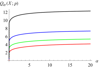
(a) $p=0.05$

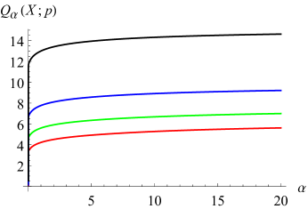
(b) $p=0.01$

Figure 1: Graphs of the quantile bounds $Q_{\alpha}(X;p)$ as functions of $\alpha$.

These graphs illustrate the general monotonicity properties of $Q_{\alpha}(X;p)$ in $\alpha$, $X$, and $p$ stated in Theorem 2.4; recall here that the Gamma distribution is (i) stochastically increasing with respect to the shape parameter $a$ and (ii) close to normality for large values of $a$. It is also seen that $Q_{\alpha}(X;p)$ varies rather little in $\alpha$, so that the quantile bounds $Q_{\alpha}(X;p)$ are not too far from the corresponding true quantiles $Q(X;p)=Q_{0}(X;p)$; cf. the somewhat similar observation made in [37, Theorem 2.8.].

In fact, it can be shown that for small values of $p$ the quantile bounds $Q_{\alpha}(X;p)$ are relatively close to the true quantiles $Q_{0}(X;p)$ whenever the right tail of the distribution of $X$ is light enough (depending on $\alpha$) and regular enough. One possible formalization of this general thesis is provided by Proposition 2.7 below, which is based on [38, Theorem 4.2 and Remark 4.3]. We shall need pertinent definitions from that paper.

Take any $r\in(0,\infty]$. Given a positive function $q$ on $\mathbb{R}$, let us say that $q(x)$ is like $x^{-r}$ if there is a positive twice differentiable function $q_{0}$ on $\mathbb{R}$ such that

$$q(x)\underset{x\to\infty}{\sim}q_{0}(x)\quad\text{and}\quad\lim_{x\to\infty}{q_{0}(x)q_{0}^{\prime\prime}(x)\over{q_{0}^{\prime}}(x)^{2}}=1+{1\over r};$$ (2.11)

as usual, we write $f\sim g$ if $f/g\to 1$. For any real $r\neq 0$, the second relation in (2.11) can be rewritten as

$$\lim_{x\to\infty}\Big{(}\frac{1}{(\ln q_{0})^{\prime}(x)}\Big{)}^{\prime}=-\frac{1}{r},$$ (2.11a)

which successively implies $\tfrac{1}{(\ln q_{0})^{\prime}(x)}\sim-\tfrac{x}{r}$, $(\ln q_{0})^{\prime}(x)\sim-\tfrac{r}{x}$, $\ln q_{0}(x)\sim-r\ln x$, and hence

$$q(x)=x^{-r+o(1)}\quad\text{as}\quad x\to\infty.$$ (2.11b)

In particular, given any $r\in(0,\infty)$, $s\in\mathbb{R}$, and $C\in(0,\infty)$,

if $$q(x)\underset{x\to\infty}{\sim}Cx^{-r}\ln^{s}x q(x) x^{-r}$$, then is like .

Also, given any $C$ and $C_{1}$ in $(0,\infty)$, $\gamma\in(0,\infty)$, and $s\in(1,\infty)$,

if  $$q(x)\underset{x\to\infty}{\sim}C\exp\{-C_{1}x^{\gamma}\} q(x)\underset{x\to\infty}{\sim}C\exp\{-C_{1}\ln^{s}x\} q(x) x^{-\infty}$$  or ,  then is like .

Moreover, if $q(x)$ is like $x^{-\infty}$, then for all $r\in(0,\infty)$ one has $q(x)=o(x^{-r})$ as $x\to\infty$.

Proposition 2.7.

1. If the r.v. $X$ is bounded from above – that is, $x_{*}<\infty$, then

   $$\lim_{p\downarrow 0}Q_{\alpha}(X;p)=\lim_{p\downarrow 0}Q_{0}(X;p)=x_{*}\in\mathbb{R}.$$ (2.12)

2. If $\operatorname{\mathsf{P}}(X\geqslant x)$ is like $x^{-r}$ for some $r\in(\alpha,\infty]$, then $x_{*}=\infty$, $Q_{\alpha}(X;p)\underset{p\downarrow 0}{\longrightarrow}\infty$, and

   $$Q_{\alpha}(X;p)\underset{p\downarrow 0}{\sim}K(r,\alpha)\,Q_{0}(X;p),$$ (2.13)

   where

   $$K(r,\alpha):=\left\{\begin{aligned} &1&&\text{\; if\; $r=\infty$},\\ &c_{r,\alpha}^{1/r}&&\text{\; if\; $r<\infty$,}\end{aligned}\right.$$ (2.14)

   $$c_{r,\alpha}:=\frac{\Gamma(\alpha+1)\Gamma(r-\alpha)}{\Gamma(r)}\frac{r^{r}}{\alpha^{\alpha}(r-\alpha)^{r-\alpha}},$$

   and $\Gamma$ is the Gamma function, given by the formula $\Gamma(\beta)=\int_{0}^{\infty}u^{\beta-1}e^{-u}{\,\operatorname{d}}u$ for $\beta>0$.

Graphs $\big{\{}\big{(}\alpha,K(r,\alpha)\big{)}\colon 0<\alpha\leqslant\min(10,0.99r),\,K(r,\alpha)\leqslant 7.5\big{\}}$ are shown here on the left: for $r=\frac{1}{2}$ (red), $r=1$ (orange), $r=2$ (green), $r=5$ (blue), $r=10$ (purple), and $r=\infty$ (black). It is seen that, if the (right) tail of the distribution of $X$ is very heavy – that is, if $r$ is comparatively small, then even for $\alpha=1$ the quantile bound $Q_{\alpha}(X;p)$ is much greater (for small $p$) than the true quantile $Q_{0}(X;p)$. However, if the tail is not very heavy – that is, if $r$ is not so small, then the graph of $K(r,\alpha)$ is very flat – that is, $Q_{\alpha}(X;p)$ varies little with $\alpha$ (if $p$ is small).

Concerning the relevance of the condition $p\downarrow 0$ in the asymptotic relations (2.12) and (2.13) in Proposition 2.7, note that small values of $p$ are of particular importance in financial practice. Indeed, values of $p$ commonly used with the so-called value-at-risk (VaR) measure – equal to the quantile $Q_{0}(X;p)$, where $X$ is the amount of financial loss – are 1% and 5% for one-day and two-week horizons, respectively [34].

As for the condition that $X$ be bounded from above in part (i) of Proposition 2.7, it is obviously fulfilled, in particular, whenever the r.v. $X$ takes only finitely many values, as is assumed e.g. in [3].

By (2.11b), if $\operatorname{\mathsf{P}}(X\geqslant x)$ is like $x^{-r}$ for some r.v. $X$ and some real $r\neq 0$, then necessarily $r>0$ – which is in accordance with the assumption $r\in(0,\infty]$ made above concerning (2.11).

Usual statistical families of continuous distributions, including the normal, log-normal, gamma, beta, Student, and Pareto families, are covered by Proposition 2.7. More specifically, part (i) of Proposition 2.7 applies to the beta family of distributions, including the uniform distribution. Part (ii) of Proposition 2.7 applies (with $r=\infty$) to the normal, log-normal, and gamma families, including the exponential family; the Student family (with $r=d$, where $d$ is the number of degrees of freedom); and Pareto family (with $r=\beta$, assuming that $\operatorname{\mathsf{P}}(X\geqslant x)=(a/x)^{\beta}$ for some $\beta$ and $a$ in $(0,\infty)$ and all real $x\geqslant a$). However, note that under the condition that $\operatorname{\mathsf{P}}(X\geqslant x)$ is like $x^{-r}$, as in part (ii) of Proposition 2.7, (2.13) is guaranteed to hold only for $\alpha\in[0,r)$. Also, in the case when $\operatorname{\mathsf{P}}(X\geqslant x)$ is like $x^{-r}$ for some $r\in(0,\infty)$, (2.13) cannot possibly hold for any $\alpha\in(r,\infty]$ – because then, by part (ii) of Proposition 1.1, (1.13), and (2.2), $Q_{\alpha}(X;p)=\infty$. So, the general tendency is that, the lighter the right tail of the distribution of $X$, the wider is the range of values of $\alpha$ for which (2.13) holds. Moreover, it appears that, the lighter the right tail of the distribution of $X$, the closer is the constant $K(r,\alpha)$ in (2.13) to $1$ and, more generally, the closer is the quantile bound $Q_{\alpha}(X;p)$ to the true quantile $Q_{0}(X;p)$.

One can also show, using [38, Remark 3.13] or [40, Remark 1.4], that (2.13) will hold – with $r=\infty$ and hence $K(r,\alpha)=1$ – for all $\alpha\in[0,\infty]$ and usual statistical families of discrete distributions, including the Poisson, geometric, and, more generally negative binomial families – because the right tails of those distributions are light enough. On the other hand, (2.12) will hold for any distributions with a bounded support, including the binomial and hypergeometric distributions.

More examples of distributions to which Proposition 2.7 is applicable can be found in [39].

***

3 Computation of the tail probability and quantile bounds

3.1 Computation of $P_{\alpha}(X;x)$

The computation of $P_{\alpha}(X;x)$ in the case $\alpha=0$ is straightforward, in view of the equality in (1.6). If $x\in[x_{*},\infty)$, then the value of $P_{\alpha}(X;x)$ is easily found by part (i) of Proposition 1.2. So, in the rest of this subsection it may be assumed that $\alpha\in(0,\infty]$ and $x\in(-\infty,x_{*})$.

In the case when $\alpha\in(0,\infty)$, using (1.5), the inequality

$$\big{(}1+\lambda(X-x)/\alpha\big{)}_{+}^{\alpha}\leqslant 2^{(\alpha-1)_{+}}\big{(}\lambda^{\alpha}X_{+}^{\alpha}+(\alpha-\lambda x)_{+}^{\alpha}\big{)}/\alpha^{\alpha},$$ (3.1)

the condition $X\in\mathscr{X}_{\alpha}$, and dominated convergence, one sees that $A_{\alpha}(X;x)(\lambda)$ is continuous in $\lambda\in(0,\infty)$ and right-continuous in $\lambda$ at $\lambda=0$ (assuming the definition (1.3) for $\lambda=0$ as well), and hence

$$P_{\alpha}(X;x)=\inf_{\lambda\in[0,\infty)}A_{\alpha}(X;x)(\lambda).$$ (3.2)

Similarly, using in place of (3.1) the inequality $e^{\lambda X}\leqslant 1+e^{\lambda_{0}X}$ whenever $0\leqslant\lambda\leqslant\lambda_{0}$, one can show that $A_{\infty}(X;x)(\lambda)$ is continuous in $\lambda\in\Lambda_{X}$ (recall (1.14)) and right-continuous in $\lambda$ at $\lambda=0$, so that (3.2) holds for $\alpha=\infty$ as well – provided that $X\in\mathscr{X}_{\infty}$. Moreover, by the Fatou lemma for the convergence in distribution [10, Theorem 5.3], $A_{\infty}(X;x)(\lambda)$ is lower-semicontinuous in $\lambda$ at $\lambda=\lambda_{*}:=\sup\Lambda_{X}$ even if $\lambda_{*}\in\mathbb{R}\setminus\Lambda_{X}$. It then follows by the convexity of $A_{\infty}(X;x)(\lambda)$ in $\lambda$ that $A_{\infty}(X;x)(\lambda)$ is left-continuous in $\lambda$ at $\lambda=\lambda_{*}$ whenever $\lambda_{*}\in\mathbb{R}$; at that, the natural topology on the set $[0,\infty]$ is used, as it is of course possible that $A_{\infty}(X;x)(\lambda_{*})=\infty$.

Since $x\in(-\infty,x_{*})$, one can find some $y\in(x,\infty)$ such that $\operatorname{\mathsf{P}}(X\geqslant y)>0$ (of course, necessarily $y\in(x,x_{*}]$); so, one can introduce

$$\lambda_{\max}:=\lambda_{\max,\alpha}:=\lambda_{\max,\alpha,X}:=\left\{\begin{aligned} &\frac{\alpha}{y-x}\,\Big{(}\frac{1}{\operatorname{\mathsf{P}}(X\geqslant y)^{1/\alpha}}-1\Big{)}&&\text{ if }\alpha\in(0,\infty),\\ &\frac{1}{y-x}\,\ln\frac{1}{\operatorname{\mathsf{P}}(X\geqslant y)}&&\text{ if }\alpha=\infty.\end{aligned}\right.$$ (3.3)

Then, by (1.3), $A_{\alpha}(X;x)(\lambda)\geqslant\operatorname{\mathsf{E}}\big{(}1+\lambda(X-x)/\alpha\big{)}_{+}^{\alpha}\,\mathsf{I}\{X\geqslant y\}\geqslant\big{(}1+\lambda(y-x)/\alpha\big{)}^{\alpha}\operatorname{\mathsf{P}}(X\geqslant y)>1$ if $\alpha\in(0,\infty)$ and $\lambda\in(\lambda_{\max,\alpha},\infty)$, and $A_{\infty}(X;x)(\lambda)\geqslant\operatorname{\mathsf{E}}e^{\lambda(X-x)}\,\mathsf{I}\{X\geqslant y\}\geqslant e^{\lambda(y-x)}\operatorname{\mathsf{P}}(X\geqslant y)>1$ if $\lambda\in(\lambda_{\max,\infty},\infty)$. So, for all $\alpha\in(0,\infty]$ one has $A_{\alpha}(X;x)(\lambda)>1\geqslant P_{\alpha}(X;x)=\inf_{\lambda\in(0,\infty)}A_{\alpha}(X;x)(\lambda)$ provided that $\lambda\in(\lambda_{\max,\infty},\infty)$, and hence

$$P_{\alpha}(X;x)=\inf_{\lambda\in[0,\lambda_{\max,\alpha}]}A_{\alpha}(X;x)(\lambda),\quad\text{if}\quad\text{$\alpha\in(0,\infty]$ and $x\in(-\infty,x_{*})$}.$$ (3.4)

Therefore and because $\lambda_{\max,\alpha}<\infty$, the minimization of $A_{\alpha}(X;x)(\lambda)$ in $\lambda$ in (3.4) in order to compute the value of $P_{\alpha}(X;x)$ can be done effectively if $\alpha\in[1,\infty]$, because in this case $A_{\alpha}(X;x)(\lambda)$ is convex in $\lambda$. At that, the positive-part moments $\operatorname{\mathsf{E}}\big{(}1+\lambda(X-x)/\alpha)_{+}^{\alpha}$, which express $A_{\alpha}(X;x)(\lambda)$ for $\alpha\in(0,\infty)$ in accordance with (1.3), can be efficiently computed using formulas in [44]; cf. e.g. [43, Section 3.2.3]. Of course, for specific kinds of distributions of the r.v. $X$, more explicit expressions for the positive-part moments can be used.

In the remaining case, when $\alpha\in(0,1)$, the function $\lambda\mapsto A_{\alpha}(X;x)(\lambda)$ cannot in general be “convexified” by any monotonic transformations in the domain and/or range of this function, and the set of minimizing values of $\lambda$ does not even have to be connected, in the following rather strong sense:

Proposition 3.1.

For any $\alpha\in(0,1)$, $p\in(0,1)$, and $x\in\mathbb{R}$, there is a r.v. $X$ (taking three distinct values) such that $P_{\alpha}(X;x)=p$ and the infimum $\inf_{\lambda\in(0,\infty)}$ in (1.5) is attained at precisely two distinct values of $\lambda\in(0,\infty)$.

Proposition 3.1 is illustrated by

Example 3.2.

Let $X$ be a r.v. taking values $-\frac{27}{11},-1,2$ with probabilities $\frac{1}{4},\frac{1}{4},\frac{1}{2}$; then $x_{*}=2$. Also let $\alpha=\frac{1}{2}$ and $x=0$, so that $x\in(-\infty,x_{*})$, and then let $\lambda_{\max}$ be as in (3.3) with $y=x_{*}=2$, so that here $\lambda_{\max}=\frac{3}{4}$. Then the minimum of $A_{\alpha}(X;0)(\lambda)$ over all real $\lambda\geqslant 0$ equals $\frac{\sqrt{3}}{2}$ and is attained at each of the two points, $\lambda=\frac{11}{54}$ and $\lambda=\frac{1}{2}$, and only at these two points. The graph $\big{\{}\big{(}\lambda,A_{1/2}(X;0)(\lambda)\big{)}\colon 0\leqslant\lambda\leqslant\lambda_{\max}\big{\}}$ is shown here on the left.

Nonetheless, effective minimization of $A_{\alpha}(X;x)(\lambda)$ in $\lambda$ in (3.4) is possible even in the case $\alpha\in(0,1)$, say by the interval method. Indeed, take any $\alpha\in(0,1)$ and write

$$A_{\alpha}(X;x)(\lambda)=A_{\alpha}^{+}(X;x)(\lambda)+A_{\alpha}^{-}(X;x)(\lambda),$$

where (cf. (1.3))

$$A_{\alpha}^{+}(X;x)(\lambda):=\operatorname{\mathsf{E}}\big{(}1+\lambda(X-x)/\alpha)_{+}^{\alpha}\,\mathsf{I}\{X\geqslant x\}\quad\text{and}\quad A_{\alpha}^{-}(X;x)(\lambda):=\operatorname{\mathsf{E}}\big{(}1+\lambda(X-x)/\alpha)_{+}^{\alpha}\,\mathsf{I}\{X<x\}.$$

Just as $A_{\alpha}(X;x)(\lambda)$ is continuous in $\lambda\in[0,\infty)$, so are $A_{\alpha}^{+}(X;x)(\lambda)$ and $A_{\alpha}^{-}(X;x)(\lambda)$. It is also clear that $A_{\alpha}^{+}(X;x)(\lambda)$ is nondecreasing and $A_{\alpha}^{-}(X;x)(\lambda)$ is nonincreasing in $\lambda\in[0,\infty)$.

So, as soon as the minimizing values of $\lambda$ are bracketed as in (3.4), one can partition the finite interval $[0,\lambda_{\max,\alpha}]$ into a large number of small subintervals $[a,b]$ with $0\leqslant a<b\leqslant\lambda_{\max,\alpha}$. For each such subinterval,

$$M_{a,b}:=\max_{\lambda\in[a,b]}A_{\alpha}(X;x)(\lambda)\leqslant A_{\alpha}^{+}(X;x)(b)+A_{\alpha}^{-}(X;x)(a),$$

$$m_{a,b}:=\min_{\lambda\in[a,b]}A_{\alpha}(X;x)(\lambda)\geqslant A_{\alpha}^{+}(X;x)(a)+A_{\alpha}^{-}(X;x)(b),$$

so that, by the continuity of $A_{\alpha}^{\pm}(X;x)(\lambda)$ in $\lambda$,

$$M_{a,b}-m_{a,b}\leqslant A_{\alpha}^{+}(X;x)(b)-A_{\alpha}^{+}(X;x)(a)+A_{\alpha}^{-}(X;x)(a)-A_{\alpha}^{-}(X;x)(b)\longrightarrow 0$$

as $b-a\to 0$, uniformly over all subintervals $[a,b]$ of the interval $[0,\lambda_{\max,\alpha}]$. Thus, one can effectively bracket the value $P_{\alpha}(X;x)=\inf_{\lambda\in[0,\lambda_{\max,\alpha}]}A_{\alpha}(X;x)(\lambda)$ with any degree of accuracy; this same approach will work, and perhaps may be sometimes useful, for $\alpha\in[1,\infty)$ as well.

3.2 Computation of $Q_{\alpha}(X;p)$

Proposition 3.3.

(Quantile bounds: Attainment and bracketing).

1. If $\alpha\in(0,\infty)$ then $\inf_{t\in T_{\alpha}}=\inf_{t\in\mathbb{R}}$ in (2.8) is attained at some $t_{\,\operatorname{opt}}\in\mathbb{R}$ and hence

   $$Q_{\alpha}(X;p)=\min_{t\in\mathbb{R}}B_{\alpha}(X;p)(t)=B_{\alpha}(X;p)(t_{\,\operatorname{opt}});$$ (3.5)

   moreover, for any

   $$s\in\mathbb{R}\quad\text{and}\quad{\tilde{p}}\in(p,1),$$

   necessarily

   $$t_{\,\operatorname{opt}}\in[t_{\min},t_{\max}],$$ (3.6)

   where

   $$t_{\max}:=B_{\alpha}(X;p)(s),\quad t_{\min}:=t_{0,\min}\wedge t_{1,\min},$$ (3.7)

   $$t_{0,\min}:=Q_{0}(X;{\tilde{p}}),\quad t_{1,\min}:=\frac{({\tilde{p}}/p)^{1/\alpha}\,t_{0,\min}-t_{\max}}{({\tilde{p}}/p)^{1/\alpha}-1}.$$ (3.8)

2. Suppose now that $\alpha=\infty$. Then $\inf_{t\in T_{\alpha}}=\inf_{t\in(0,\infty)}$ in (2.8) is attained and hence

   $$Q_{\infty}(X;p)=\min_{t\in(0,\infty)}B_{\infty}(X;p)(t)$$

   unless

   $$x_{*}<\infty\quad\text{and}\quad p\leqslant p_{*},$$ (3.9)

   where $x_{*}$ and $p_{*}$ are as in (1.16). On the other hand, if conditions (3.9) hold then $B_{\infty}(X;p)(t)$ is strictly increasing in $t>0$ and hence $\inf_{t\in T_{\alpha}}=\inf_{t\in(0,\infty)}$ in (2.8) is not attained; rather,

   $$Q_{\infty}(X;p)=\inf_{t>0}B_{\infty}(X;p)(t)=B_{\infty}(X;p)(0+)=x_{*}.$$

For instance, in the case when $\alpha=0.5$, $p=0.05$, and $X$ has the Gamma distribution with the shape and scale parameters equal to $2.5$ and $1$, respectively, Proposition 3.3 yields $t_{\min}>4.01$ (using ${\tilde{p}}=0.095$) and $t_{\max}<6.45$.

When $\alpha=0$, the quantile bound $Q_{\alpha}(X;p)$ is simply the quantile $Q(X;p)$, which can be effectively computed by formula (2.3), since the tail probability $\operatorname{\mathsf{P}}(X>x)$ is monotone in $x$. Next, as was noted in the proof of Theorem 2.4, $B_{\alpha}(X;p)(t)$ is convex in $t$ when $\alpha\in[1,\infty]$, which provides for an effective computation of $Q_{\alpha}(X;p)$ by formula (2.8).

Therefore, it remains to consider the computation – again by formula (2.8) – of $Q_{\alpha}(X;p)$ for $\alpha\in(0,1)$. In such a case, as in Subsection 3.1, one can use an interval method. As soon as the minimizing values of $t$ are bracketed as in (3.6), one can partition the finite interval $[t_{\min},t_{\max}]$ into a large number of small subintervals $[a,b]$ with $t_{\min}\leqslant a<b\leqslant t_{\max}$. For each such subinterval,

$$M_{a,b}:=\max_{t\in[a,b]}B_{\alpha}(X;p)(t)\leqslant b+p^{-1/\alpha}\,\|(X-a)_{+}\|_{\alpha},$$

$$m_{a,b}:=\min_{t\in[a,b]}B_{\alpha}(X;p)(t)\geqslant a+p^{-1/\alpha}\,\|(X-b)_{+}\|_{\alpha},$$

so that, by the continuity of $\|(X-t)_{+}\|_{\alpha}$ in $t$,

$$M_{a,b}-m_{a,b}\leqslant b-a+p^{-1/\alpha}\,(\|(X-a)_{+}\|_{\alpha}-\|(X-b)_{+}\|_{\alpha})\longrightarrow 0$$

as $b-a\to 0$, uniformly over all subintervals $[a,b]$ of the interval $[t_{\min},t_{\max}]$. Thus, one can effectively bracket the value $Q_{\alpha}(X;p)=\inf_{t\in\mathbb{R}}B_{\alpha}(X;p)(t)$; this same approach will work, and perhaps may be useful, for $\alpha\in[1,\infty)$ as well.

***

If $\alpha\in(1,\infty)$ then, by part (ii) of Proposition 3.6 and part (i) of Proposition 3.3, the set $\mathop{\operatorname{argmin}}\limits_{t\in\mathbb{R}}B_{\alpha}(X;p)(t)$ is a singleton one; that is, there is exactly one minimizer $t\in\mathbb{R}$ of $B_{\alpha}(X;p)(t)$. If $\alpha=1$ then $B_{\alpha}(X;p)(t)=B_{1}(X;p)(t)$ is convex, but not strictly convex, in $t$, and the set $\mathop{\operatorname{argmin}}\limits_{t\in\mathbb{R}}B_{\alpha}(X;p)(t)$ of all minimizers of $B_{\alpha}(X;p)(t)$ in $t$ coincides with the set of all $(1-p)$-quantiles of $X$, as mentioned at the conclusion of the derivation of the identity (3.10). Thus, if $\alpha=1$, then the set $\mathop{\operatorname{argmin}}\limits_{t\in\mathbb{R}}B_{\alpha}(X;p)(t)$ may in general be, depending on $p$ and the distribution of $X$, a nonzero-length closed interval. Finally, if $\alpha\in(0,1)$ then, in general, the set $\mathop{\operatorname{argmin}}\limits_{t\in\mathbb{R}}B_{\alpha}(X;p)(t)$ does not have to be connected:

Proposition 3.4.

For any $\alpha\in(0,1)$, $p\in(0,1)$, and $x\in\mathbb{R}$, there is a r.v. $X$ (taking three distinct values) such that $Q_{\alpha}(X;p)=x$ and the infimum $\inf_{t\in T_{\alpha}}=\inf_{t\in\mathbb{R}}$ in (2.8) is attained at precisely two distinct values of $t$.

Proposition 3.4 follows immediately from Proposition 3.1, by the duality (2.10) and the change-of-variables identity $A_{\alpha}(X;x)(\lambda)={\tilde{A}}_{\alpha}(X;x)(x-\alpha/\lambda)$ for $\alpha\in(0,\infty)$, used to establish (1.7)–(1.9). At that, $\lambda\in(0,\infty)$ is one of the two minimizers of $A_{\alpha}(X;x)(\lambda)$ in Proposition 3.1 if and only if $t:=x-\alpha/\lambda$ is one of the two minimizers of $B_{\alpha}(X;p)(t)$ in Proposition 3.4.

Proposition 3.1 is illustrated by the following example, which is obtained from Example 3.2 by the same duality (2.10).

Example 3.5.

As in Example 3.2, let $\alpha=\frac{1}{2}$ and let $X$ be a r.v. taking values $-\frac{27}{11},-1,2$ with probabilities $\frac{1}{4},\frac{1}{4},\frac{1}{2}$. Also let $p=\frac{\sqrt{3}}{2}$. Then the minimum of $B_{\alpha}(X;p)(t)$ over all real $t$ equals $0$ and is attained at each of the two points, $t=-\frac{27}{11}$ and $t=-1$, and only at these two points. The graph $\big{\{}\big{(}t,B_{1/2}\big{(}X;\frac{\sqrt{3}}{2}\big{)}(t)\big{)}\colon\break-3\leqslant t\leqslant 3\big{\}}$ is shown here on the left. The minimizing values of $t$ here, $-\frac{27}{11}$ and $-1$, are related with the minimizing values of $\lambda$ in Example 3.2, $\frac{11}{54}$ and $\frac{1}{2}$, by the mentioned formula $t=x-\alpha/\lambda$ (here with $x=0$ and $\alpha=\frac{1}{2}$).

***

In the case $\alpha=1$, an expression of $Q_{\alpha}(X;p)$ can be given in terms of the true $(1-p)$-quantile $Q(X;p)$:

$$Q_{1}(X;p)=Q(X;p)+\tfrac{1}{p}\,\operatorname{\mathsf{E}}\big{(}X-Q(X;p)\big{)}_{+}.$$ (3.10)

That the expression for $Q_{1}(X;p)$ in (2.8) coincides with the one in (3.10) was proved in [52, Theorem 1] for absolutely continous r.v.’s $X$ and in [35, page 273] and [53, Theorem 10] in general. For the readers’ convenience, let us present here the following brief proof of (3.10). For all real $h>0$ and $t\in\mathbb{R}$ one has

$$(X-t)_{+}-(X-t-h)_{+}=h\,\mathsf{I}\{X>t\}-(t+h-X)\,\mathsf{I}\{t<X<t+h\}.$$

It follows that the right derivative of the convex function $t\mapsto t+\|(X-t)_{+}\|_{1}/p$ at any point $t\in\mathbb{R}$ is $1-\operatorname{\mathsf{P}}(X>t)/p$, which, by (2.3), is $\leqslant 0$ if $t<Q(X;p)$ and $>0$ if $t>Q(X;p)$. Hence, $Q(X;p)$ is a minimizer in $t\in\mathbb{R}$ of $t+\|(X-t)_{+}\|_{1}/p$, and thus (3.10) follows by (2.8). It is also seen now that any $(1-p)$-quantile of $X$ is a minimizer in $t\in\mathbb{R}$ of $t+\|(X-t)_{+}\|_{1}/p$ as well, and $Q(X;p)$ is the largest of these minimizers.

As was shown in [53], the expression for $Q_{1}(X;p)$ in (3.10) can be rewritten as a conditional expectation:

$$Q_{1}(X;p)=Q(X;p)+\operatorname{\mathsf{E}}\big{(}X-Q(X;p)\big{|}X\geqslant Q(X;p),\,U\geqslant\delta\big{)}=\operatorname{\mathsf{E}}\big{(}X|X\geqslant Q(X;p),\,U\geqslant\delta\big{)},$$ (3.11)

where $U$ is any r.v. which independent of $X$ and uniformly distributed on the interval $[0,1]$, $\delta:=\delta(X;p):=d\,\mathsf{I}\{X=Q(X;p)\}$, and $d$ is any real number in the interval $[0,1]$ such that

$$\operatorname{\mathsf{P}}\!\big{(}X\geqslant Q(X;p)\big{)}-p=\operatorname{\mathsf{P}}\big{(}X=Q(X;p)\big{)}\,d;$$

such a number $d$ always exists. Thus, the r.v. $U$ is used to split the possible atom of the distribution of $X$ at the quantile point $Q(X;p)$ in order to make the randomized tail probability $\operatorname{\mathsf{P}}\!\big{(}X\geqslant Q(X;p),\,U\geqslant\delta\big{)}$ exactly equal to $p$. Of course, in the absence of such an atom, one can simply write

$$Q_{1}(X;p)=Q(X;p)+\operatorname{\mathsf{E}}\big{(}X-Q(X;p)\big{|}X\geqslant Q(X;p)\big{)}=\operatorname{\mathsf{E}}\big{(}X|X\geqslant Q(X;p)\big{)}.$$ (3.12)

However, as pointed out in [52, 53], a variational formula such as (2.8) has a distinct advantage over such ostensibly explicit formulas as (3.10) and (3.11), since (2.8) allows for incorporation into specialized optimization problems, with additional restrictions, say on the distribution of $X$; cf. e.g. [52, Theorem 2].

Nonetheless, let us obtain an extension of the representation (3.10), valid for all $\alpha\in[1,\infty)$. In accordance with [43, Proposition 3.2], consider

$$x_{**}:=x_{**,X}:=\sup\big{(}(\operatorname{supp}X)\setminus\{x_{*}\}\big{)}\in[-\infty,x_{*}]\subseteq[-\infty,\infty].$$ (3.13)

The following proposition will be useful.

Proposition 3.6.

1. If $\alpha\in[1,\infty]$ then $B_{\alpha}(X;p)(t)$ is convex in $t\in T_{\alpha}$.

2. If $\alpha\in(1,\infty)$ then $B_{\alpha}(X;p)(t)$ is strictly convex in $t\in(-\infty,x_{**}]\cap\mathbb{R}$.

3. $B_{\infty}(X;p)(t)$ is strictly convex in $t\in\{s\in(0,\infty)\colon\operatorname{\mathsf{E}}e^{X/s}<\infty\}$ unless $\operatorname{\mathsf{P}}(X=c)=1$ for some $c\in\mathbb{R}$.

Suppose at this point that $\alpha\in[1,\infty)$. By part (i) of Proposition 3.3 (stated in Section 3), the minimum-attainment set

$$\mathop{\operatorname{argmin}}\limits_{t\in\mathbb{R}}B_{\alpha}(X;p)(t):=\{t\in\mathbb{R}\colon B_{\alpha}(X;p)(t)=Q_{\alpha}(X;p)\}$$ (3.14)

is nonempty and bounded. Also, this set is closed, by the continuity of $B_{\alpha}(X;p)(t)$ in $t\in\mathbb{R}$. Therefore, the definition

$${}_{\alpha-1}Q(X;p):=\max\mathop{\operatorname{argmin}}\limits_{t\in\mathbb{R}}B_{\alpha}(X;p)(t)$$ (3.15)

makes sense, and

$${}_{\alpha-1}Q(X;p)\in\mathbb{R};$$ (3.16)

thus, ${}_{\alpha-1}Q(X;p)$ is the largest value of $t$ minimizing $B_{\alpha}(X;p)(t)$. Moreover, in the case when $\alpha=1$ this largest minimizer is

$${}_{0}Q(X;p)=Q_{0}(X;p),$$ (3.17)

the largest $(1-p)$-quantile of $X$, as stated at the end of the paragraph containing (3.10) and its proof. Thus, indeed the representation (3.10) is extended to all $\alpha\in[1,\infty)$:

$$Q_{\alpha}(X;p)={}_{\alpha-1}Q(X;p)+p^{-1/\alpha}\,\big{\|}\big{(}X-{}_{\alpha-1}Q(X;p)\big{)}_{+}\big{\|}_{\alpha}.$$ (3.18)

Further properties of ${}_{\alpha-1}Q(X;p)$ are presented in

Proposition 3.7.

Suppose that $\alpha\in[1,\infty)$. Then the following statements are true.

1. Computation of ${}_{\alpha-1}Q(X;p)$:

   1. If $p\in(0,p_{*}]\cap(0,1)$ then ${}_{\alpha-1}Q(X;p)=x_{*}=Q_{0}(X;p)$, where $x_{*}$ is as in (1.16).

   2. Suppose here that $\alpha\in(1,\infty)$ and $p\in(p_{*},1)$. Then ${}_{\alpha-1}Q(X;p)=t_{\alpha,p}$, where $t_{\alpha,p}$ is the only root $t\in(-\infty,x_{*})$ of the equation ${}_{\alpha-1}P(X;t)=p$ and, again for $t\in(-\infty,x_{*})$,

      $$\kern-28.45274pt{}_{\alpha-1}P(X;t):=\Big{(}\frac{\|(X-t)_{+}\|_{\alpha-1}}{\|(X-t)_{+}\|_{\alpha}\ \ \;}\Big{)}^{(\alpha-1)\alpha}=\frac{\operatorname{\mathsf{E}}^{\alpha}(X-t)_{+}^{\alpha-1}}{\operatorname{\mathsf{E}}^{\alpha-1}(X-t)_{+}^{\alpha}}=\operatorname{\mathsf{P}}(X>t)\,\frac{\operatorname{\mathsf{E}}^{\alpha}\big{(}(X-t)^{\alpha-1}|X>t\big{)}}{\operatorname{\mathsf{E}}^{\alpha-1}\big{(}(X-t)^{\alpha}|X>t\big{)}}.$$ (3.19)

      Moreover,

      $${}_{\alpha-1}Q(X;p)=t_{\alpha,p}\in(-\infty,x_{**}).$$ (3.20)

      Furthermore, for all $t\in(-\infty,x_{*})$ one has ${}_{\alpha-1}P(X;t)\leqslant\operatorname{\mathsf{P}}(X>t)\leqslant P_{0}(X;t)$, and also ${}_{\alpha-1}P(X;t)\to\operatorname{\mathsf{P}}(X>t)$ as $\alpha\downarrow 1$ (assuming that $X\in\mathscr{X}_{\alpha}$ for some $\alpha\in(1,\infty)$); in addition, ${}_{\alpha-1}P(X;t)<\operatorname{\mathsf{P}}(X>t)$ for all $t\in(-\infty,x_{**})$.

2. ${}_{\alpha-1}Q(X;p)$ is nonincreasing in $p\in(0,1)$ and ${}_{\alpha-1}Q(X;p)=x_{*}=\mbox{\emph{const}}$ for $p\in(0,p_{*}]\cap(0,1)$. Moreover, if $\alpha\in(1,\infty)$ then ${}_{\alpha-1}Q(X;p)$ is strictly decreasing in $p\in[p_{*},1)$ and continuous in $p\in(p_{*},1)$; at that, ${}_{\alpha-1}Q(X;p)\underset{p\downarrow p_{*}}{\longrightarrow}x_{**}$ and ${}_{\alpha-1}Q(X;p)\underset{p\uparrow 1}{\longrightarrow}-\infty$.

3. ${}_{\alpha-1}Q(X;p)$ is nonincreasing in $\alpha\in[1,\infty)$ in the sense that ${}_{\beta-1}Q(X;p)\leqslant{}_{\alpha-1}Q(X;p)$ if $1\leqslant\alpha<\beta<\infty$ and $X\in\mathscr{X}_{\beta}$; in particular,

   $${}_{\alpha-1}Q(X;p)\leqslant{}_{0}Q(X;p)=Q_{0}(X;p)=Q(X;p),$$ (3.21)

   if $X\in\mathscr{X}_{\alpha}$. More specifically, if $p\in(0,p_{*}]\cap(0,1)$, $1\leqslant\alpha<\infty$, and $X\in\mathscr{X}_{\alpha}$, then ${}_{\alpha-1}Q(X;p)=x_{*}$; if $p\in(p_{*},1)$, $1\leqslant\alpha<\beta<\infty$, and $X\in\mathscr{X}_{\beta}$, then ${}_{\beta-1}Q(X;p)<{}_{\alpha-1}Q(X;p)$. Moreover, if $p\in(p_{*},1)$ and $X\in\mathscr{X}_{\infty}$, then ${}_{\alpha-1}Q(X;p)\underset{\alpha\uparrow\infty}{\longrightarrow}-\infty$.

4. ${}_{\alpha-1}Q(X;p)$ is consistent: ${}_{\alpha-1}Q(c;p)=c$ for all $c\in\mathbb{R}$.

5. ${}_{\alpha-1}Q(X;p)$ is positive-homogeneous: ${}_{\alpha-1}Q(\kappa X;p)=\kappa\,{}_{\alpha-1}Q(X;p)$ for all $\kappa\in[0,\infty)$.

6. ${}_{\alpha-1}Q(X;p)$ is translation-invariant: ${}_{\alpha-1}Q(X+c;p)={}_{\alpha-1}Q(X;p)+c$ for all $c\in\mathbb{R}$.

7. ${}_{\alpha-1}Q(X;p)$ is partially monotonic: ${}_{\alpha-1}Q(X;p)\leqslant{}_{\alpha-1}Q(c;p)$ if $X\leqslant c$ for some $c\in\mathbb{R}$; also, ${}_{\alpha-1}Q(X;p)\leqslant{}_{\alpha-1}Q(X+c;p)$ for any $c\in[0,\infty)$.

8. However, for any $\alpha\in(1,\infty)$ and any $p\in(0,1)$, ${}_{\alpha-1}Q(X;p)$ is not monotonic in all $X\in\mathscr{X}_{\alpha}$.

9. Consequently, for any $\alpha\in[1,\infty)$ and any $p\in(0,1)$, ${}_{\alpha-1}Q(X;p)$ is not subadditive or convex in all $X\in\mathscr{X}_{\alpha}$.

By (3.21), ${}_{\alpha-1}Q(X;p)$ is a lower bound on the true $(1-p)$-quantile $Q(X;p)$ of $X$. Therefore and in view of part (i) of Proposition 3.7, ${}_{\alpha-1}Q(X;p)$ may be referred to as the lower $(\alpha-1,1-p)$-quantile of the r.v. $X$.

Example 3.8.

Parts (ii) and (iii) of Proposition 3.7 are illustrated in the picture here on the left, with graphs $\big{\{}\big{(}p,\,{}_{\alpha-1}Q(X;p)\big{)}\colon\break 0<p<0.99\big{\}}$ for a r.v. $X=X_{a,b}$ as in Examples 1.3 and 2.2, with the same $a=1$ and $b=3$, and the values of $\alpha$ equal $1$ (green), $2$ (orange), and $5$ (red). Note that here $x_{*}=b=3$ and $x_{**}=-a=-1$.

***

One may conclude this section by an obvious but oftentimes rather useful observation that – even when a minimizing value of $\lambda$ or $t$ in formulas (1.5), (1.7), or (2.8) is not identified quite perfectly – one still obtains, by those formulas, an upper bound on $P_{\alpha}(X;x)$ or $Q_{\alpha}(X;p)$ and hence on the true tail probability $\operatorname{\mathsf{P}}(X\geqslant x)$ or the true quantile $Q(X;p)$, respectively.

4 Implications for risk control/inequality modeling in finance/economics

In financial literature – see e.g. [35, 53, 24], the quantile bounds $Q_{0}(X;p)$ and $Q_{1}(X;p)$ are known as the value-at-risk and conditional value-at-risk, denoted as ${\,\operatorname{VaR}}_{p}(X)$ and ${\,\operatorname{CVaR}}_{p}(X)$, respectively:

$$Q_{0}(X;p)={\,\operatorname{VaR}}_{p}(X)\quad\text{and}\quad Q_{1}(X;p)={\,\operatorname{CVaR}}_{p}(X);$$ (4.1)

here, $X$ is interpreted as a priori uncertain potential loss. The value of $Q_{1}(X;p)$ is also known as the expected shortfall (ES) [2], average value-at-risk (AVaR) [47], and expected tail loss (ETL) [26]. As indicated in [53], at least in the case when there is no atom at the quantile point $Q(X;p)$, the quantile bound $Q_{1}(X;p)$ is also called the “mean shortfall” [28], whereas the difference $Q_{1}(X;p)-Q(X;p)$ is referred to as “mean excess loss” [17, 6].

Greater values of $\alpha$ correspond to greater sensitivity to risk; cf. e.g. [19]. For instance, let $X$ and $Y$ denote the potential losses corresponding to two different investments portfolios. Suppose that there are mutually exclusive events $E_{1}$ and $E_{2}$ and real numbers $p_{*}\in(0,1)$ and $\delta\in(0,1)$ such that (i) $\operatorname{\mathsf{P}}(E_{1})=\operatorname{\mathsf{P}}(E_{2})=p_{*}/2$, (ii) the loss of either portfolio is $0$ if the event $E_{1}\cup E_{2}$ does not occur, (iii) the loss of the $X$-portfolio is $1$ if the event $E_{1}\cup E_{2}$ occurs, and (iv) the loss of the $Y$-portfolio is $1-\delta$ if the event $E_{1}$ occurs, and it is $1+\delta$ if the event $E_{2}$ occurs. Thus, the r.v. $X$ takes values $0$ and $1$ with probabilities $1-p_{*}$ and $p_{*}$, and the r.v. $Y$ takes values $0$, $1-\delta$, and $1+\delta$ with probabilities $1-p_{*}$, $p_{*}/2$, and $p_{*}/2$, respectively. So, $\operatorname{\mathsf{E}}X=\operatorname{\mathsf{E}}Y$, that is, the expected losses of the two portfolios are the same. Clearly, the distribution of $X$ is less dispersed than that of $Y$, both intuitively and also in the formal sense that $X\overset{\alpha+1}{\leqslant}Y$ for all $\alpha\in[1,\infty]$. Therefore, everyone will probably say that the $Y$-portfolio is riskier than the $X$-portfolio. However, for any $p\in(p_{*},1)$ it is easy to see, by (2.3), that $Q_{0}(X;p)=0=Q_{0}(Y;p)$ and hence, in view of (3.10), $Q_{1}(Y;p)=\frac{1}{p}\,\operatorname{\mathsf{E}}Y=\frac{p_{*}}{p}=\frac{1}{p}\,\operatorname{\mathsf{E}}X=Q_{1}(X;p)$. Using also the continuity of $Q_{\alpha}(\cdot;p)$ in $p$, as stated in Theorem 2.4, one concludes that the $Q_{1}(\cdot;p)={\,\operatorname{CVaR}}_{p}(\cdot)$ risk value of the riskier $Y$-portfolio is the same as that of the less risky $X$-portfolio for all $p\in[p_{*},1)$. Such indifference (which may also be referred to as insensitivity to risk) may generally be considered “an unwanted characteristic” [23, pages 36, 48].

Let us now show that, in contrast with the risk measure $Q_{1}(\cdot;p)={\,\operatorname{CVaR}}_{p}(\cdot)$, the value of $Q_{\alpha}(\cdot;p)$ is sensitive to risk for all $\alpha\in(1,\infty)$ and all $p\in(0,1)$; that is, for all such $\alpha$ and $p$ and for the losses $X$ and $Y$ as above, $Q_{\alpha}(Y;p)>Q_{\alpha}(X;p)$. Indeed, take any $\alpha\in(1,\infty)$. By (1.16) and (3.13), $x_{*,X}=1$, $p_{*,X}=p_{*}$, $x_{*,Y}=1+\delta$, $x_{**,Y}=1-\delta$, and $p_{*,Y}=p_{*}/2$. If $p\in(0,p_{*}/2]$ then, by part (ii) of Proposition 2.1, $Q_{\alpha}(Y;p)=x_{*,Y}=1+\delta>1=x_{*,X}=Q_{\alpha}(X;p)$. If now $p\in(p_{*}/2,1)$ then, by (3.20), $t_{Y}:={}_{\alpha-1}Q(Y;p)\in(-\infty,x_{**,Y})=(-\infty,1-\delta)$. Also, by strict version of Jensen’s inequality and the strict convexity of $u^{\alpha}$ in $u\in[0,\infty)$, $B_{\alpha}(X;p)(t)=t+p^{-1/\alpha}\|X-t\|_{\alpha}<t+p^{-1/\alpha}\|Y-t\|_{\alpha}=B_{\alpha}(Y;p)(t)$ for all $t\in(-\infty,1-\delta]$. So, by (3.18) and (2.8), $Q_{\alpha}(Y;p)=B_{\alpha}(Y;p)(t_{Y})>B_{\alpha}(X;p)(t_{Y})\geqslant Q_{\alpha}(X;p)$. Thus, it is checked that $Q_{\alpha}(Y;p)>Q_{\alpha}(X;p)$ for all $\alpha\in(1,\infty)$ and all $p\in(0,1)$.

The above example is illustrated in Figure 2, for $p_{*}=0.1$ and $\delta=0.6$. It is seen that the sensitivity of the measure $Q_{\alpha}(\cdot;p)$ to risk (reflected especially by the gap between the red and blue lines for $p\in[p_{*},1)=[0.1,\,1)$) increases from the zero sensitivity when $\alpha=1$ to an everywhere positive sensitivity when $\alpha=2$ to an everywhere greater positive sensitivity when $\alpha=5$.

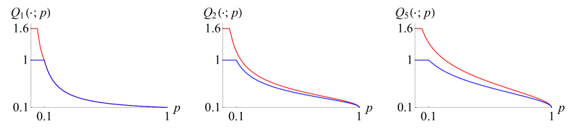
Figure 2: Sensitivity of $Q_{\alpha}(\cdot;p)$ to risk, depending on the value of $\alpha$: graphs $\big{\{}\big{(}p,Q_{\alpha}(X;p)\big{)}\colon 0<p<1\big{\}}$ (blue) and $\big{\{}\big{(}p,Q_{\alpha}(Y;p)\big{)}\colon 0<p<1\big{\}}$ (red) for $\alpha=1$ (left panel), $\alpha=2$ (middle panel), and $\alpha=5$ (right panel).

***

Based on an extensive and penetrating discussion of methods of measurement of market and nonmarket risks, Artzner et al [3] concluded that, for a risk measure to be effective in risk regulation and management, it has to be coherent, in the sense that it possess the translation invariance, subadditivity, positive homogeneity, and monotonicity properties. In general, a risk measure, say $\hat{\rho}$, is a mapping of a linear space of real-valued r.v.’s on a given probability space into $\mathbb{R}$. The probability space (say $\Omega$) was assumed to be finite in [3]. More generally, one could allow $\Omega$ to be infinite, and then it is natural to allow $\hat{\rho}$ to take values $\pm\infty$ as well. In [3], the r.v.’s (say $Y$) in the argument of the risk measure were called risks but at the same time interpreted as “the investor’s future net worth”. Then the translation invariance was defined in [3] as the identity $\hat{\rho}(Y+rt)=\hat{\rho}(Y)-t$ for all r.v.’s $Y$ and real numbers $t$, where $r$ is a positive real number, interpreted as the rate of return. We shall, however, follow Pflug [35], who considers a risk measure (say $\rho$) as a function of the potential cost/loss, say $X$, and then defines the translation invariance of $\rho$, quite conventionally, as the identity $\rho(X+c)=\rho(X)+c$ for all r.v.’s $X$ and real numbers $c$. The approaches in [3] and [35] are equivalent to each other, and the correspondence between them can be given by the formulas $\rho(X)=r\hat{\rho}(Y)=r\hat{\rho}(-X)$, $X=-Y$, and $c=-rt$. The positive homogeneity as defined in [3] can be stated as the identity $\rho(\lambda X)=\lambda\rho(X)$ for all r.v.’s $X$ and real numbers $\lambda\geqslant 0$.

Corollary 4.1.

For each $\alpha\in[1,\infty]$, the quantile bound $Q_{\alpha}(\cdot;p)$ is a coherent risk measure.

This follows immediately from Theorem 2.4.

The usually least trivial of the four properties characterizing the coherence is the subadditivity of a risk measure – which, in the presence of the positive homogeneity, is equivalent to the convexity, as was pointed out earlier in this paper. As is well known and also discussed above, the value-at-risk measure ${\,\operatorname{VaR}}_{p}(X)$ is translation invariant, positive homogeneous, and monotone (in $X$), but it fails to be subadditive. Quoting [53, page 1458]: “The coherence of [${\,\operatorname{CVaR}}_{p}(X)$] is a formidable advantage not shared by any other widely applicable measure of risk yet proposed.” Corollary 4.1 above addresses this problem by providing an entire infinite family of coherent risk measures, indexed by $\alpha\in[1,\infty]$, including ${\,\operatorname{CVaR}}_{p}(X)=Q_{1}(X;p)$ just as one member of the family.

Theorem 2.4 also provides additional monotonicity and other useful properties of the spectrum of risk measures $Q_{\alpha}(\cdot;p)$. The terminology we use to name some of these properties differs from the corresponding terminology used in [3]. Namely, what we referred to as the “sensitivity” in Theorem 2.4 corresponds to the “relevance” in [3]. Also, in the present paper the “model-independence” means that the risk measure depends on the potential loss only through the distribution of the loss, rather than on the way to model the “states of nature”, on which the loss may depend. In contrast, in [3] a measure of risk is considered “model-free” if it does not depend, not only on modeling the “states of nature”, but, to a possibly large extent, on the distribution of the loss. The “model-independence” property is called “law-invariance” in [21, Section 12.1.2], where the consistency property was referred to as “constancy”. An example of such a “model-free” risk measure is given by the Securities and Exchange Commission (SEC) rules, described e.g. in [3, Subsection 3.2]; this measure of risk depends only on the set of all possible representations of the investment portfolio in question as a portfolio of long call spreads, that is, pairs of the form (a long call, a short call). If a measure of risk is not “model-free”, then it is called “model-dependent” in [3].

***

Yitzhaki [58] utilized the Gini mean difference – which had prior to that been mainly used as a measure of economic inequality – to construct, somewhat implicitly, a measure of risk; this approach was further developed in [14, 11]. If (say) a r.v. $X$ is thought of as the income of randomly selected person in a certain state, then the Gini mean difference can be defined by the formula

$$G_{H}(X):=\operatorname{\mathsf{E}}H(|X-{\tilde{X}}|),$$

where ${\tilde{X}}$ is an independent copy of $X$ and $H\colon[0,\infty)\to\mathbb{R}$ is a measurable function, usually assumed to be nonnegative and such that $H(0)=0$; clearly, given the function $H$, the Gini mean difference $G_{H}(X)$ depends only on the distribution of the r.v. $X$. So, if $H(u)$ is considered, for any $u\in[0,\infty)$, as the measure of inequality between two individuals with incomes $x$ and $y$ such that $|x-y|=u$, then the Gini mean difference $\operatorname{\mathsf{E}}H(|X-{\tilde{X}}|)$ is the mean $H$-inequality in income between two individuals selected at random (and with replacement, thus independently of each other). The most standard choice for $H$ is the identity function ${\,\operatorname{id}}$, so that $H(u)={\,\operatorname{id}}(u)=u$ for all $u\in[0,\infty)$. Based on the measure-of-inequality $G_{H}$, one can define the risk measure

$$R_{H}(X):=\operatorname{\mathsf{E}}X+G_{H}(X)=\operatorname{\mathsf{E}}X+\operatorname{\mathsf{E}}H(|X-{\tilde{X}}|),$$ (4.2)

where now the r.v. $X$ is interpreted as the uncertain loss on a given investment, with the term $G_{H}(X)=\operatorname{\mathsf{E}}H(|X-{\tilde{X}}|)$ then possibly interpreted as a measure of the uncertainty. Clearly, when there is no uncertainty, so that the loss $X$ is in fact a nonrandom real constant, then the measure $G_{H}(X)$ of the uncertainty is $0$, assuming that $H(0)=0$. If $X\sim N(\mu,\sigma^{2})$ (that is, $X$ is normally distributed with mean $\mu$ and standard deviation $\sigma>0$) and $H=\kappa{\,\operatorname{id}}$ for some positive constant $\kappa$, then $R_{H}(X)=\mu+\frac{2\kappa}{\sqrt{\pi}}\,\sigma$, a linear combination of the mean and the standard deviation, so that in such a case we find ourselves in the realm of the Markowitz mean-variance risk-assessment framework.

It is assumed that $R_{H}(X)$ is defined when both expected values in the last expression in (4.2) are defined and are not infinite values of opposite signs – so that these two expected values could be added, as needed in (4.2).

It is clear that $R_{H}(X)$ is translation-invariant. Moreover, $R_{H}(X)$ is convex in $X$ if the function $H$ is convex and nondecreasing. Further, if $H=\kappa{\,\operatorname{id}}$ for some positive constant $\kappa$, then $R_{H}(X)$ is also positive-homogeneous.

It was shown in [58], under an additional technical condition, that $R_{H}(X)$ is nondecreasing in $X$ with respect to the stochastic dominance of order $1$ if $H=\frac{1}{2}{\,\operatorname{id}}$. Namely, the result obtained in [58] is that if $X\mathrel{\overset{\mathrm{st}}{\leqslant}}Y$ and the distribution functions $F$ and $G$ of $X$ and $Y$ are such that $F-G$ changes sign only finitely many times on $\mathbb{R}$, then $R_{\frac{1}{2}{\,\operatorname{id}}}(X)\leqslant R_{\frac{1}{2}{\,\operatorname{id}}}(Y)$. A more general result was obtained in [14], which can be stated as follows: in the case when the function $H$ is differentiable, $R_{H}(X)$ is nondecreasing in $X$ with respect to the stochastic dominance of order $1$ if and only if $|H^{\prime}|\leqslant\frac{1}{2}$. Cf. also [11]. The proof in [14] was rather long and involved; in addition, it used a previously obtained result of [27]. Here we are going to give (in Appendix A) a very short, direct, and simple proof of the more general

Proposition 4.2.

The risk measure $R_{H}(X)$ is nondecreasing in $X$ with respect to the stochastic dominance of order $1$ if and only if the function $H$ is $\frac{1}{2}$-Lipschitz: $|H(x)-H(y)|\leqslant\frac{1}{2}\,|x-y|$ for all $x$ and $y$ in $[0,\infty)$.

In Proposition 4.2, it is not assumed that $H\geqslant 0$ or that $H(0)=0$. Of course, if $H$ is differentiable, then the $\frac{1}{2}$-Lipschitz condition is equivalent to the condition $|H^{\prime}|\leqslant\frac{1}{2}$ in [14].

The risk measure $R_{H}(X)$ was called mean-risk (M-R) in [11].

It follows from [14] or Proposition 4.2 above that the risk measure $R_{\kappa{\,\operatorname{id}}}(X)$ is coherent for any $\kappa\in[0,\frac{1}{2}]$. In fact, based on Proposition 4.2, one can rather easily show more:

Proposition 4.3.

The risk measure $R_{H}(X)$ is coherent if and only if $H=\kappa{\,\operatorname{id}}$ for some $\kappa\in[0,\frac{1}{2}]$.

It is possible to indicate a relation – albeit rather indirect – of the risk measure $R_{H}(X)$, defined in (4.2), with the quantile bounds $Q_{\alpha}(X;p)$. Indeed, introduce

$$\hat{Q}_{\alpha}(X;p)=\operatorname{\mathsf{E}}X+p^{-1/\alpha}\,\big{\|}(X-\operatorname{\mathsf{E}}X)_{+}\big{\|}_{\alpha},$$ (4.3)

assuming $\operatorname{\mathsf{E}}X$ exists in $\mathbb{R}$. By (2.8)–(2.9), $\hat{Q}_{\alpha}(X;p)$ is another majorant of $Q_{\alpha}(X;p)$, obtained by using $t=\operatorname{\mathsf{E}}X$ in (2.8) as a surrogate of the minimizing value of $t$.

The term $p^{-1/\alpha}\,\big{\|}(X-\operatorname{\mathsf{E}}X)_{+}\big{\|}_{\alpha}$ in (4.3) is somewhat similar to the Gini mean-difference term $\operatorname{\mathsf{E}}H(|X-{\tilde{X}}|)$, at least when $\alpha=1$ and (the distribution of) the r.v. $X$ is symmetric about its mean.

Moreover, if the distribution of $X-\operatorname{\mathsf{E}}X$ is symmetric and stable with index $\gamma\in(1,2]$, then $\hat{Q}_{1}(X;p)=R_{\kappa{\,\operatorname{id}}}(X)$ with $\kappa=2^{-1-1/\gamma}/p$.

One may want to compare the two considered kinds of coherent measures of risk/inequality, $R_{\kappa{\,\operatorname{id}}}(X)$ for $\kappa\in[0,\frac{1}{2}]$ and $Q_{\alpha}(X;p)$ for $\alpha\in[1,\infty]$ and $p\in(0,1)$. It appears that the latter measure is more flexible, as it depends on two parameters ($\alpha$ and $p$) rather than one just one parameter ($\kappa$). Moreover, as Proposition 2.7 shows, rather generally $Q_{\alpha}(X;p)$ retains a more or less close relation with the quantile $Q_{0}(X;p)$ – which, recall, is the widely used value-at-risk (VaR). On the other hand, recall here that, in contrast with the VaR, $Q_{\alpha}(X;p)$ is coherent for $\alpha\in[1,\infty]$. However, both of these kinds of coherent measures appear useful, each in its own manner, representing two different ways to express risk/inequality.

Formulas (4.2) and (4.3) can be considered special instances of the general relation between risk measures and measures of inequality established in [54]. Let $\mathscr{X}_{\operatorname{\mathsf{E}}}$ be a convex cone of real-valued r.v. $X\in\mathscr{X}$ with a finite mean $\operatorname{\mathsf{E}}X$ such that $\mathscr{X}_{\operatorname{\mathsf{E}}}$ contains all real constants.

Largely following [54], let us say a coherent real-valued risk measure $R\colon\mathscr{X}_{\operatorname{\mathsf{E}}}\to(-\infty,\infty]$ is strictly expectation-bounded if $R(X)>\operatorname{\mathsf{E}}X$ for all $X\in\mathscr{X}_{\operatorname{\mathsf{E}}}$. (Note that here the r.v. $X$ represents the loss, whereas in [54] it represents the gain; accordingly, $X$ in this paper corresponds to $-X$ in [54]; also, in [54] the cone $\mathscr{X}_{\operatorname{\mathsf{E}}}$ was taken to be the space $\mathscr{L}^{2}$.) In view of Theorem 2.4 and part (vii) of Proposition 2.1, it follows that $Q_{\alpha}(X;p)$ is a coherent and strictly expectation-bounded risk measure if $\alpha\in[1,\infty]$. Also (cf. [54, Definition 1 and Proposition 1]), let us say that a mapping $D\colon\mathscr{X}_{\operatorname{\mathsf{E}}}\to[0,\infty]$ is a deviation measure if $D$ is subadditive, positive-homogeneous, and nonnegative with $D(X)=0$ if and only if $\operatorname{\mathsf{P}}(X=c)=1$ for some real constant $c$; here $X$ is any r.v. in $\mathscr{X}_{\operatorname{\mathsf{E}}}$. Next (cf. [54, Definition 2]), let us say that a deviation measure $D\colon\mathscr{X}_{\operatorname{\mathsf{E}}}\to[0,\infty]$ is upper-range dominated if $D(X)\leqslant\sup\operatorname{supp}X-\operatorname{\mathsf{E}}X$ for all $X\in\mathscr{X}_{\operatorname{\mathsf{E}}}$. Then (cf. [54, Theorem 2]), the formulas

$$D(X)=R(X-\operatorname{\mathsf{E}}X)\quad\text{and}\quad R(X)=\operatorname{\mathsf{E}}X+D(X)$$ (4.4)

provide a one-to-one correspondence between all coherent strictly expectation-bounded risk measures $R\colon\mathscr{X}_{\operatorname{\mathsf{E}}}\to(-\infty,\infty]$ and all upper-range dominated deviation measures $D\colon\mathscr{X}_{\operatorname{\mathsf{E}}}\to[0,\infty]$.

In particular, it follows that the risk measure $\hat{Q}_{\alpha}(\cdot;p)$, defined by formula (4.3), is coherent for all $\alpha\in[1,\infty]$ and all $p\in(0,\infty)$. It also follows that $X\mapsto Q_{\alpha}(X-\operatorname{\mathsf{E}}X;p)$ is a deviation measure. As was noted, $\hat{Q}_{\alpha}(X;p)$ is a majorant of $Q_{\alpha}(X;p)$. In contrast with $Q_{\alpha}(X;p)$, in general $\hat{Q}_{\alpha}(X;p)$ will not have such a close hereditary relation with the true quantile $Q_{0}(X;p)$ as e.g. the ones given in Proposition 2.7. For instance, if $\operatorname{\mathsf{P}}(X\geqslant x)$ is like $x^{-\infty}$ then, by (2.13)–(2.14), $Q_{\alpha}(X;p)\underset{p\downarrow 0}{\sim}Q_{0}(X;p)$ for each $\alpha\in[0,\infty]$, whereas $\hat{Q}_{\infty}(X;p)=\infty$ for all real $p>0$. On the other hand, in distinction with the definition (4.3) of $\hat{Q}_{\alpha}(X;p)$, the expression (2.8) for $Q_{\alpha}(X;p)$ requires minimization in $t$; however, that minimization will add comparatively little to the complexity of the problem of minimizing $Q_{\alpha}(X;p)$ subject to a usually large number of restrictions on the distribution of $X$; cf. again e.g. [52, Theorem 2].

One may also consider the following modification of $\hat{Q}_{\alpha}(X;p)$, which is still a majorant of $Q_{\alpha}(X;p)$, but is closer (than $\hat{Q}_{\alpha}(X;p)$ is) to the true quantile $Q_{0}(X;p)$ – at least when $p\in(0,1)$ is close enough to $1$ (recall part (ii) of Proposition 3.7):

$$\hat{Q}^{<}_{\alpha}(X;p):=\inf_{t\in(-\infty,\operatorname{\mathsf{E}}X]}B_{\alpha}(X;p)(t);$$ (4.5)

cf. (2.8).

The risk measure $\hat{Q}^{<}_{\alpha}(\cdot;p)$ is coherent and strictly expectation-bounded given the condition $\alpha\in[1,\infty]$, which will be assumed in this paragraph. The proof of the translation invariance, positive homogeneity, and subadditivity properties of $\hat{Q}^{<}_{\alpha}(\cdot;p)$ is almost the same as the proof of these properties of $Q_{\alpha}(\cdot;p)$, listed in Theorem 2.4. Then, to prove the monotonicity of $Q_{\alpha}(\cdot;p)$ (with respect to the order $\mathrel{\overset{\mathrm{st}}{\leqslant}}$), it is enough, in view of the subadditivity of $\hat{Q}^{<}_{\alpha}(\cdot;p)$ and as in the proof of [54, Theorem 2], to show that $X\leqslant 0$ implies $\hat{Q}^{<}_{\alpha}(X;p)\leqslant 0$, which obtains indeed, because $\hat{Q}^{<}_{\alpha}(X;p)\leqslant\hat{Q}_{\alpha}(X;p)$ and $\hat{Q}_{\alpha}(X;p)\leqslant\hat{Q}_{\alpha}(0;p)=0$ if $X\leqslant 0$. Finally, $\hat{Q}^{<}_{\alpha}(\cdot;p)$ is strictly expectation-bounded, because it majorizes $Q_{\alpha}(\cdot;p)$, which is strictly expectation-bounded, as noted.

***

Recalling (1.28) and following [31, 32, 33], one may also consider $-F_{-X}^{(-\alpha)}(p)$ as a measure of risk. Here one will need the following semigroup identity, given in [31, (8a)] (cf. e.g. [38, Remark 3.7]):

$$F_{X}^{(-\alpha)}(p)=\frac{1}{\Gamma(\alpha-\nu)}\int_{0}^{p}(p-u)^{\alpha-\nu-1}F_{X}^{(-\nu)}(u){\,\operatorname{d}}u$$ (4.6)

whenever $0<\nu<\alpha<\infty$. The following proposition is well known.

Proposition 4.4.

If the r.v. $X$ is nonnegative then

$$F_{X}^{(-2)}(p)=L_{X}(p)=-p{\,\operatorname{CVaR}}_{p}(-X),$$ (4.7)

where $L_{X}$ is the Lorenz curve function, given by the formula

$$L_{X}(p):=\int_{0}^{p}F_{X}^{-1}(u){\,\operatorname{d}}u.$$ (4.8)

Indeed, the first equality in (4.7) is the special case of the identity (4.6) with $\alpha=2$ and $\nu=1$, and the second equality in (4.7) follows by [30, part (i) of Theorem 3.1], identity (2.8) for $\alpha=1$, and the second identity in (4.1). Cf. [25, Theorem 2] and [4, 29].

Using (4.6) with $\nu=2$, $\alpha+1$ in place of $\alpha$, and $-X$ in place of $X$ together with Proposition 4.4, one has

$$-F_{-X}^{(-\alpha-1)}(p)=\frac{1}{\Gamma(\alpha-1)}\int_{0}^{p}(p-u)^{\alpha-2}\,u{\,\operatorname{CVaR}}_{u}(X){\,\operatorname{d}}u$$ (4.9)

for any $\alpha\in(1,\infty)$. Since ${\,\operatorname{CVaR}}_{u}(X)$ is a coherent risk measure, it now follows that, as noted in [32], $-F_{-X}^{(-\alpha-1)}(p)$ is a coherent risk measure as well, again for $\alpha\in(1,\infty)$; by (4.7), this conclusion will hold for $\alpha=1$. However, one should remember that the expression $F_{X}^{(-\alpha)}(p)$ was defined only when the r.v. $X$ is nonnegative (and otherwise some of the crucial considerations above will not hold). Thus, the risk measure $-F_{-X}^{(-\alpha-1)}(p)$ is defined only if $X\leqslant 0$ almost surely.

In view of (4.9), this risk measure is a mixture of the coherent risk measures ${\,\operatorname{CVaR}}_{u}(X)$ and thus a member of the general class of the so-called spectral risk measures [1], which are precisely the mixtures, over the values $u\in(0,1)$, of the risk measures ${\,\operatorname{CVaR}}_{u}(X)$; thus, all spectral risk measures are automatically coherent. However, in general such measures will lack such an important variational representation as the one given by formula (2.8) for the risk measure $Q_{\alpha}(X;p)$. Of course, for any “mixing” nonnegative Borel measure $\mu$ on the interval $(0,1)$ and the corresponding spectral risk measure

$${\,\operatorname{CVaR}}_{\mu}(X):=\int_{(0,1)}{\,\operatorname{CVaR}}_{u}(X)\,\mu({\,\operatorname{d}}u),$$

one can write

$${\,\operatorname{CVaR}}_{\mu}(X)=\int_{(0,1)}\inf_{t\in\mathbb{R}}\big{(}t+\tfrac{1}{u}\,\|(X-t)_{+}\|_{1}\big{)}\,\mu({\,\operatorname{d}}u),$$ (4.10)

in view of (4.1) and (2.8)–(2.9). However, in contrast with (2.8), the minimization (in $t\in\mathbb{R}$) in (4.10) needs in general to be done for each of the infinitely many values of $u\in(0,1)$. If the r.v. $X$ takes only finitely many values, then the expression of ${\,\operatorname{CVaR}}_{\mu}(X)$ in (4.10) can be rewritten as a finite sum, so that the minimization in $t\in\mathbb{R}$ will be needed only for finitely many values of $u$; cf. e.g. the optimization problem on page 8 in [32].

On the other hand, one can of course consider arbitrary mixtures in $p\in(0,1)$ and/or $\alpha\in[1,\infty)$ of the risk measures $Q_{\alpha}(X;p)$. Such mixtures will automatically be coherent. Also, all mixtures of the measures $Q_{\alpha}(X;p)$ in $p$ will be nondecreasing in $\alpha$, and all mixtures of $Q_{\alpha}(X;p)$ in $\alpha$ will be nonincreasing in $p$.

Deviation measures such as the ones studied in [54] and discussed in the paragraph containing (4.4) can be used as measures of economic inequality if the r.v. $X$ models, say, the random income/wealth – defined as the income/wealth of an (economic) unit chosen at random from a population of such units. Then, according to the one-to-one correspondence given by (4.4), coherent risk measures $R$ translate into deviation measures $D$, and vice versa.

However, the risk measures $Q_{\alpha}(\cdot;p)$ themselves can be used to express certain aspects of economic inequality directly, without translation into deviation measures. For instance, if $X$ stands for the random wealth then the statement $Q_{1}(X;0.01)=30\operatorname{\mathsf{E}}X$ formalizes the common kind of expression “the wealthiest 1% own 30% of all wealth”, provided that the wealthiest 1% can be adequately defined, say as follows: there is a threshold wealth value $t$ such that the number of units with wealth greather than or equal to $t$ is $0.01N$, where $N$ is the number of units in the entire population. Then (cf. (3.12)) $0.01\,N\,Q_{1}(X;0.01)=0.01\,N\,\operatorname{\mathsf{E}}(X|X\geqslant t)=N\operatorname{\mathsf{E}}X\,\mathsf{I}\{X\geqslant t\}=0.30\,N\operatorname{\mathsf{E}}X$, whence indeed $Q_{1}(X;0.01)=30\operatorname{\mathsf{E}}X$. Similar in spirit expressions of economic inequality in terms of $Q_{\alpha}(X;p)$ can be provided for all $\alpha\in(0,\infty)$. For instance, suppose now that $X$ stands for the annual income of a randomly selected household, whereas $x$ is a particular annual household income level in question. Then, in view of (2.8)–(2.9), the inequality $Q_{\alpha}(X;p)\geqslant x$ means that for any (potential) annual household income level $t$ less than the maximum annual household income level $x_{*,X}$ in the population, the conditional $\alpha$-mean $\operatorname{\mathsf{E}}\big{(}(X-t)^{\alpha}|X>t\big{)}^{1/\alpha}$ of the excess $(X-t)_{+}$ of the random income $X$ over $t$ is no less than $\big{(}\frac{p}{\operatorname{\mathsf{P}}(X>t)}\big{)}^{1/\alpha}$ times the excess $(x-t)_{+}$ of the income level $x$ over $t$. Of course, the conditional $\alpha$-mean $\operatorname{\mathsf{E}}\big{(}(X-t)^{\alpha}|X>t\big{)}^{1/\alpha}$ is increasing in $\alpha$. Thus, using the measure $Q_{\alpha}(X;p)$ of economic inequality with a greater value of $\alpha$ means treating high values of the economic variable $X$ in a more progressive/sensitive manner. One may also note here that the above interpretation of the inequality $Q_{\alpha}(X;p)\geqslant x$ is a “synthetic” statement in the sense that is provides information concerning all values of potential interest of the threshold annual household income level $t$.

Not only the upper bounds $Q_{\alpha}(X;p)$ on the quantile $Q(X;p)$, but also the upper bounds $\operatorname{\mathsf{P}}_{\alpha}(X;x)$ on the tail probability $\operatorname{\mathsf{P}}(X\geqslant x)$ may be considered measures of risk/inequality. Indeed, if $X$ is interpreted as the potential loss, then the tail probability $\operatorname{\mathsf{P}}(X\geqslant x)$ corresponds to the classical safety-first (SF) risk measure; see e.g. [55, 22].

Using variational formulas – of which formulas (1.5), (1.7), and (2.8) are examples – to define or compute measures of risk is not peculiar to the present paper. Indeed, as mentioned previously, the special case of (2.8) with $\alpha=1$ is the well-known variational representation (3.10) of ${\,\operatorname{CVaR}}$, obtained in [52, 35, 53]. The risk measure given by the SEC rules [3, Subsection 3.2], also mentioned before, is another example where the calculations are done, in effect, according to a certain minimization formula, which is somewhat implicit and complicated in that case.

One can now list some of the advantages of the risk/inequality measures $P_{\alpha}(X;x)$ and $Q_{\alpha}(X;p)$:

• $P_{\alpha}(X;x)$ and $Q_{\alpha}(X;p)$ are three-way monotonic and three-way stable – in $\alpha$, $p$, and $X$.

• The monotonicity in $X$ is graded continuously in $\alpha$, resulting in various, controllable degrees of sensitivity of $P_{\alpha}(X;x)$ and $Q_{\alpha}(X;p)$ to financial risk/economic inequality.

• $x\mapsto P_{\alpha}(X;x)$ is the tail-function of a certain probability distribution.

• $Q_{\alpha}(X;p)$ is a $(1-p)$-percentile of that probability distribution.

• For small enough values of $p$ the quantile bounds $Q_{\alpha}(X;p)$ are close enough to the corresponding true quantiles $Q(X;p)$ provided that the right tail of the distribution of $X$ is light enough and regular enough, depending on $\alpha$.

• $P_{\alpha}(X;x)$ and $Q_{\alpha}(X;p)$ are solutions to mutually dual optimizations problems, which can be comparatively easily incorporated into more specialized optimization problems, with additional restrictions, say on the distribution of the random variable $X$.

• $P_{\alpha}(X;x)$ and $Q_{\alpha}(X;p)$ are effectively computable.

• Even when the corresponding minimizer is not identified quite perfectly – one still obtains an upper bound on the risk/inequality measures $P_{\alpha}(X;x)$ or $Q_{\alpha}(X;p)$.

• Optimal upper bounds on $P_{\alpha}(X;x)$ and hence on $Q_{\alpha}(X;p)$ over important classes of r.v.’s $X$ represented (say) as sums of independent r.v.’s $X_{i}$ with restrictions on moments of the $X_{i}$’s and/or sums of such moments can be given, as is done e.g. in [39, 7, 8, 41, 42, 43].

• The quantile bounds $Q_{\alpha}(X;p)$ with $\alpha\in[1,\infty]$ constitute a spectrum of coherent measures of financial risk and economic inequality.

• The r.v.’s $X$ of which the measures $P_{\alpha}(X;x)$ and $Q_{\alpha}(X;p)$ are taken are allowed to take values of both signs. In particular, if, in a context of economic inequality, $X$ is interpreted as the net amount of assets belonging to a randomly chosen economic unit, then a negative value of $X$ corresponds to a unit with more liabilities than paid-for assets. Similarly, if $X$ denotes the loss on a financial investment, then a negative value of $X$ will obtain when there actually is a net gain.

Some of these advantages, and especially their totality, appear to be unique to the bounds proposed here.

Acknowledgment. I am pleased to thank Emmanuel Rio for the mentioned communication [50], which also included a reference to [24] and in fact sparked the study presented here.

Appendix A Proofs

Proof of Proposition 1.1.

Part (i) of the proposition follows immediately from (1.5), (1.3), and (1.2).

Parts (ii) and (iii) follow by (1.7)–(1.9). Indeed, $\operatorname{\mathsf{E}}(X-t)_{+}^{\alpha}\geqslant\operatorname{\mathsf{E}}X_{+}^{\alpha}/2^{(\alpha-1)_{+}}-|t|^{\alpha}=\infty$ for all real $x$ and $t$ if $\operatorname{\mathsf{E}}X_{+}^{\alpha}=\infty$, and $\operatorname{\mathsf{E}}e^{(X-x)/t}=e^{-x/t}\operatorname{\mathsf{E}}e^{X/t}=\infty$ for all real $x$ and $t>0$ if $\operatorname{\mathsf{E}}e^{\lambda X}=\infty$ for all real $\lambda>0$.

Concerning part (iv) of Proposition 1.1, assume indeed that $\alpha\in(0,\infty)$ and $\operatorname{\mathsf{E}}X_{+}^{\alpha}<\infty$. Then, for any $x>0$, (1.7)–(1.9) imply $P_{\alpha}(X;x)\leqslant\frac{\operatorname{\mathsf{E}}X_{+}^{\alpha}}{x_{+}^{\alpha}}\to 0$ as $x\to\infty$. On the other hand, obviously $P_{\alpha}(X;x)\geqslant 0$ for all real $x$. So, indeed, $P_{\alpha}(X;x)\to 0$ as $x\to\infty$.

By (3.2), (1.3), and (1.1), $P_{\alpha}(X;x)\leqslant A_{\alpha}(X;x)(0)=h_{\alpha}(0)=1$. On the other hand, by (1.6), $P_{\alpha}(X;(-\infty)+)\geqslant P_{0}(X;(-\infty)+)=1$. So, indeed $P_{\alpha}(X;(-\infty)+)=1$.

Thus, part (iv) of Proposition 1.1 is proved.

The proof of part (v) is rather similar to that of part (iv). Assume indeed that $\alpha=\infty$ and $\operatorname{\mathsf{E}}e^{\lambda_{0}X}<\infty$ for some real $\lambda_{0}>0$. Then $P_{\infty}(X;x)\leqslant\operatorname{\mathsf{E}}e^{\lambda_{0}(X-x)}=e^{-\lambda_{0}x}\operatorname{\mathsf{E}}e^{\lambda_{0}X}\to 0$ as $x\to\infty$. Since $P_{\infty}(X;x)\geqslant 0$ for all real $x$, one indeed has $P_{\infty}(X;x)\to 0$ as $x\to\infty$.

As for the proof of the statement that $P_{\alpha}(X;x)\to 1$ as $x\to-\infty$ for $\alpha=\infty$, it is the same as the corresponding proof for $\alpha\in(0,\infty)$.

Thus, part (v) of Proposition 1.1 is proved as well. ∎

Proof of Proposition 1.2.

(i) Let us first verify part (i). For $\alpha=0$, this follows immediately from the equality in (1.6) and the definitions in (1.16).

Take then any $\alpha\in(0,\infty]$. Take indeed any $x\in[x_{*},\infty)$.

If $\alpha\in(0,\infty)$ and $u\in(-\infty,x_{*}]$, then $h_{\alpha}\big{(}\lambda(u-x)\big{)}=\big{(}1+\lambda(u-x)/\alpha\big{)}_{+}^{\alpha}\underset{\lambda\to\infty}{\longrightarrow}\,\mathsf{I}\{u=x\}$; so, by (1.3), the condition $X\in\mathscr{X}_{\alpha}$, and dominated convergence, $A_{\alpha}(X;x)(\lambda)=\operatorname{\mathsf{E}}h_{\alpha}\big{(}\lambda(X-x)\big{)}\underset{\lambda\to\infty}{\longrightarrow}\operatorname{\mathsf{P}}(X=x)$. The case $\alpha=\infty$ is similar: $A_{\infty}(X;x)(\lambda)=\operatorname{\mathsf{E}}e^{\lambda(X-x)}\,\mathsf{I}\{X\leqslant x\}\underset{\lambda\to\infty}{\longrightarrow}\operatorname{\mathsf{P}}(X=x)$.

So, by (1.5), $P_{\alpha}(X;x)\leqslant\operatorname{\mathsf{P}}(X=x)=\operatorname{\mathsf{P}}(X\geqslant x)$. Now part (i) of Proposition 1.2 follows in view of the inequality in (1.6).

(ii) Part (ii) of Proposition 1.2 follows because, by (1.6) and (1.16), $P_{\alpha}(X;x)\geqslant\operatorname{\mathsf{P}}(X\geqslant x)>0$ for all $x\in(-\infty,x_{*})$.

(iii) Concerning part (iii) of Proposition 1.2, consider first the case $\alpha\in(0,\infty)$. Then, by (1.7), the function

$$(-\infty,x_{*}]\cap\mathbb{R}\ni x\mapsto P_{\alpha}(X;x)^{-1/\alpha}\in[0,\infty]$$ (A.1)

is the pointwise supremum, in $t\in(-\infty,x_{*})$, of the family of continuous convex functions $(-\infty,x_{*}]\cap\mathbb{R}\ni x\mapsto\frac{(x-t)_{+}}{\|(X-t)_{+}\|_{\alpha}}\in[0,\infty]$. So, the function (A.1) is convex. It is also finite on the interval $(-\infty,x_{*})$, by part (ii) of Proposition 1.2. So, the function (A.1) is continuous on $(-\infty,x_{*})$. Moreover, this function is lower-semicontinuous and nondecreasing, and hence continuous at the point $x_{*}$, in the case when $x_{*}\in\mathbb{R}$. Thus, the function (A.1) is continuous on the entire set $(-\infty,x_{*}]\cap\mathbb{R}$, with respect to the natural topologies on $(-\infty,x_{*}]\cap\mathbb{R}$ and $[0,\infty]$.

The case $\alpha=\infty$ is considered quite similarly. Here, instead of (A.1), one works with the function

$$(-\infty,x_{*}]\cap\mathbb{R}\ni x\mapsto-\ln P_{\alpha}(X;x)\in(-\infty,\infty],$$ (A.2)

which is the pointwise supremum, in real $\lambda>0$ such that $\operatorname{\mathsf{E}}e^{\lambda X}<\infty$, of the family of continuous convex (in fact, affine) functions $\mathbb{R}\ni x\mapsto-\ln\operatorname{\mathsf{E}}e^{\lambda(X-x)}=\lambda x-\ln\operatorname{\mathsf{E}}e^{\lambda X}\in(-\infty,\infty]$. (Actually, the values of the latter family of functions are all real, for $\lambda>0$ such that $\operatorname{\mathsf{E}}e^{\lambda X}<\infty$, whereas all the values of the function (A.2) are in $[0,\infty]$; however, here we take the union, $(-\infty,\infty]$, of the sets $\mathbb{R}$ and $[0,\infty]$ as an interval which is guaranteed to contain all possible values of all the convex functions under consideration.) Here we also use the standard conventions $\ln 0:=-\infty$ and $e^{-\infty}:=0$; concerning the continuity of functions with values in the set $(-\infty,\infty]$, we use the natural topology on this set.

(iv) Let us now turn to part (iv) of Proposition 1.2. Consider first the case $\alpha\in(0,\infty)$. Then, since the map $[0,\infty]\ni r\mapsto r^{-\alpha}$ is continuous, it follows by part (iii) of Proposition 1.2 that $P_{\alpha}(X;x)$ is indeed continuous in $x\in(-\infty,x_{*})$ and left-continuous in $x$ at $x_{*}$ if $x_{*}\in\mathbb{R}$. The case $\alpha=\infty$ is quite similar; here, instead of the map $[0,\infty]\ni r\mapsto r^{-\alpha}$, one should use the continuous map $(-\infty,\infty]\ni r\mapsto e^{-r}$.

(v) That the function $\mathbb{R}\ni x\mapsto P_{\alpha}(X;x)$ is left-continuous follows immediately from parts (iv) and (i) if $\alpha\in(0,\infty]$, and from the equality in (1.6) if $\alpha=0$.

(vi) That $x_{\alpha}$ is nondecreasing in $\alpha\in[0,\infty]$ follows immediately from the definition of $x_{\alpha}$ in (1.17) and (1.13). That $x_{\alpha}<\infty$ follows because, by (1.15), $P_{\alpha}(X;x)\to 0<1$ as $x\to\infty$.

(vii) If $x\in(-\infty,\operatorname{\mathsf{E}}X]$ then, by Jensen’s inequality,

$$A_{1}(X;x)(\lambda)=\operatorname{\mathsf{E}}\big{(}1+\lambda(X-x)\big{)}_{+}\geqslant\big{(}1+\lambda(\operatorname{\mathsf{E}}X-x)\big{)}_{+}\geqslant 1$$

for all $\lambda\in(0,\infty)$, whence, by (1.5), $P_{1}(X;x)\geqslant 1$, and so, by (1.13), $P_{\alpha}(X;x)\geqslant 1$ for all $\alpha\in[1,\infty]$.

On the other hand, if $x\in(\operatorname{\mathsf{E}}X,\infty)$ then $A_{\infty}(X;x)(\lambda)=\operatorname{\mathsf{E}}e^{\lambda(X-x)}<\operatorname{\mathsf{E}}e^{0(X-x)}=1$ for all $\lambda$ in a right neighborhood of $0$ – because the right derivative of $\operatorname{\mathsf{E}}e^{\lambda(X-x)}$ in $\lambda$ at $\lambda=0$ is $\operatorname{\mathsf{E}}(X-x)<0$; therefore, $P_{\infty}(X;x)<1$, and so, again by (1.13), $P_{\alpha}(X;x)<1$ for all $\alpha\in[1,\infty]$.

This completes the proof of part (vii) of Proposition 1.2.

(viii) By part (i) of Proposition 1.2, $P_{\alpha}(X;x)=0<1$ for all $x\in(x_{*},\infty)$, so that $(x_{*},\infty)\subseteq E_{\alpha}(1)$, which implies $x_{\alpha}\leqslant x_{*}$.

Let us show that $x_{\alpha}=x_{*}$ if and only if $p_{*}=1$. By the definition of $x_{\alpha}$ in (1.17) and (1.15), $P_{\alpha}(X;x)=1$ for all $x\in(-\infty,x_{\alpha})$. So, by part (v) of Proposition 1.2 and the inequality $x_{\alpha}<\infty$ in part (vi) of Proposition 1.2,

$$x_{\alpha}>-\infty\implies P_{\alpha}(X;x_{\alpha})=\lim_{x\uparrow x_{\alpha}}P_{\alpha}(X;x)=1.$$ (A.3)

If now $x_{\alpha}=x_{*}$, then $x_{\alpha}>-\infty$ by the definition of $x_{*}$ in (1.16); so, by part (i) of Proposition 1.2 and (A.3), $p_{*}=P_{\alpha}(X;x_{*})=P_{\alpha}(X;x_{\alpha})=1$, which proves the implication $x_{\alpha}=x_{*}\implies p_{*}=1$. Vice versa, suppose that $p_{*}=1$. Then necessarily $x_{*}\in\mathbb{R}$. Moreover, by part (i) of Proposition 1.1 and part (i) of Proposition 1.2, for all $x\in(-\infty,x_{*}]$ one has $P_{\alpha}(X;x)\geqslant P_{\alpha}(X;x_{*})=p_{*}=1$, so that $E_{\alpha}(1)\subseteq(x_{*},\infty)$ and hence $x_{\alpha}\geqslant x_{*}$. Now the conclusion $x_{\alpha}=x_{*}$ follows by the already established inequality $x_{\alpha}\leqslant x_{*}$.

(ix) By the definition of $x_{\alpha}$ in (1.17) and part (i) of Proposition 1.1, the set $E_{\alpha}(1)$ is an interval with endpoints $x_{\alpha}$ and $\infty$. So, by the inequality $x_{\alpha}<\infty$ in part (vi) of Proposition 1.2, $E_{\alpha}(1)\neq\emptyset$. Thus, to verify part (ix) of Proposition 1.2, it is enough to show that $x_{\alpha}\notin E_{\alpha}(1)$. If $x_{\alpha}=-\infty$ then this follows immediately from the definition of $E_{\alpha}(p)$ in (1.18) as a subset of $\mathbb{R}$, and if $x_{\alpha}>-\infty$ then the same conclusion follows by (A.3).

(x) Part (x) of Proposition 1.2 follows immediately from part (ix) of Proposition 1.2 and the inequality $P_{\alpha}(X;x)\leqslant 1$, which latter in turn follows by (1.15).

(xi) Consider first the case $\alpha\in(0,\infty)$. By part(i) of Proposition 1.1 and (1.15), the function (A.1) is nondecreasing, from the value $1$ at $-\infty$. It is easy to see that these conditions, together with the convexity of the function (A.1), imply that this function is strictly increasing on the set $\{x\in(-\infty,x_{*}]\cap\mathbb{R}\colon 1<P_{\alpha}(X;x)^{-1/\alpha}<\infty\}$. In view of part (ii) of Proposition 1.2, this implies that the function $x\mapsto P_{\alpha}(X;x)$ is strictly decreasing on the set $(-\infty,x_{*})\cap\{x\in\mathbb{R}\colon P_{\alpha}(X;x)<1\}$, which is the same as $(x_{\alpha},x_{*})$, by part (ix) of Proposition 1.2. The conclusion in part (xi) of Proposition 1.2 for $\alpha\in(0,\infty)$ now follows by its part (iv). The case $\alpha=\infty$ is quite similar, where one uses, instead of (A.1), the function (A.2), whose limit at $-\infty$ is $0$. ∎

Proof of Proposition 1.4.

Let $\alpha$ and a sequence $(\alpha_{n})$ be indeed as in Proposition 1.4. If $x\in[x_{*},-\infty)$ then the desired conclusion $P_{\alpha_{n}}(X;x)\to P_{\alpha}(X;x)$ follows immediately from part (i) of Proposition 1.2. Therefore, assume in the rest of the proof of Proposition 1.4 that

$$x\in(-\infty,x_{*}).$$ (A.4)

Then (3.4) takes place and, by (3.3), $\lambda_{\max,\alpha}$ is continuous in $\alpha\in(0,\infty]$. So,

$$\lambda^{*}:=\sup_{n}\lambda_{\max,\alpha_{n}}\in[0,\infty)$$ (A.5)

and

$$P_{\gamma}(X;x)=\inf_{\lambda\in[0,\lambda_{*}]}A_{\gamma}(X;x)(\lambda)\quad\text{for all}\quad\gamma\in\{\alpha\}\cup\{\alpha_{n}\colon n\in\mathbb{N}\}.$$ (A.6)

Also, by (1.3), (1.2), the inequality (3.1) for $\alpha\in(0,\infty)$, the condition $X\in\mathscr{X}_{\beta}$, and dominated convergence,

$$A_{\alpha_{n}}(X;x)(\lambda)\to A_{\alpha}(X;x)(\lambda).$$ (A.7)

Hence, by (1.5), $\limsup_{n}P_{\alpha_{n}}(X;x)\leqslant\limsup_{n}A_{\alpha_{n}}(X;x)(\lambda)=A_{\alpha}(X;x)(\lambda)$ for all $\lambda\in[0,\infty)$, whence, again by (1.5),

$$\limsup_{n}P_{\alpha_{n}}(X;x)\leqslant P_{\alpha}(X;x).$$ (A.8)

So, the case $\alpha=0$ of Proposition 1.4 follows by (1.6).

If $\alpha\in(0,1]$ then for any $\kappa$ and $\lambda$ such that $0\leqslant\kappa<\lambda<\infty$ one has

$$|A_{\alpha}(X;x)(\lambda)-A_{\alpha}(X;x)(\kappa)|\leqslant(\lambda-\kappa)^{\alpha}\operatorname{\mathsf{E}}(X-x)_{+}^{\alpha}/\alpha^{\alpha}+(\lambda-\kappa)^{\alpha/2}/\alpha^{\alpha}+\operatorname{\mathsf{P}}\big{(}(x-X)_{+}>\tfrac{1}{\sqrt{\lambda-\kappa}}\big{)};$$ (A.9)

this follows because

$$0\leqslant(1+\lambda u/\alpha)_{+}^{\alpha}-(1+\kappa u/\alpha)_{+}^{\alpha} \leqslant(\lambda-\kappa)^{\alpha}u^{\alpha}/\alpha^{\alpha}\quad\text{if}\quad u\geqslant 0,$$

$$0\leqslant(1+\kappa u/\alpha)_{+}^{\alpha}-(1+\lambda u/\alpha)_{+}^{\alpha} \leqslant\min\big{(}1,(\lambda-\kappa)^{\alpha}|u|^{\alpha}/\alpha^{\alpha}\big{)}$$

$$\leqslant(\lambda-\kappa)^{\alpha/2}/\alpha^{\alpha}+\,\mathsf{I}\{|u|>\tfrac{1}{\sqrt{\lambda-\kappa}}\}\quad\text{if}\quad u<0.$$

If now $\alpha\in(0,1)$ then (say, by cutting off an initial segment of the sequence $(\alpha_{n})$) one may assume that $\beta\in(0,1)$, and then, by (A.9) with $\alpha_{n}$ in place of $\alpha$, the sequence $\big{(}A_{\alpha_{n}}(X;x)(\lambda)\big{)}$ is equicontinuous in $\lambda\in[0,\infty)$, uniformly in $n$. Therefore, by (A.5) and the Arzelà–Ascoli theorem, the convergence in (A.7) is uniform in $\lambda\in[0,\lambda^{*}]$ and hence the conclusion $P_{\alpha_{n}}(X;x)\to P_{\alpha}(X;x)$ follows by (A.6) – in the case when $\alpha\in(0,1)$.

Quite similarly, the same conclusion holds if $\alpha=1=\beta$; that is, $P_{\alpha}(X;x)$ is left-continuous in $\alpha$ at the point $\alpha=1$ provided that $\operatorname{\mathsf{E}}X_{+}<\infty$.

It remains to consider the case when $\alpha\in[1,\infty]$ and $\alpha_{n}\geqslant 1$ for all $n$. Then, by the definition in (1.1), the functions $h_{\alpha}$ and $h_{\alpha_{n}}$ are convex and hence, by (1.3), $A_{\alpha}(X;x)(\lambda)$ and $A_{\alpha_{n}}(X;x)(\lambda)$ are convex in $\lambda\in[0,\infty)$. Then the conclusion $P_{\alpha_{n}}(X;x)\to P_{\alpha}(X;x)$ follows by [45, Corollary 3], the condition $X\in\mathscr{X}_{\beta}$, (A.6), and (A.5). ∎

Proof of Proposition 1.5.

This is somewhat similar to the proof of Proposition 1.4. One difference here is the use of the uniform integrability condition, which, in view of (1.3), (3.1), and the condition $X\in\mathscr{X}_{\alpha}$, implies (see e.g. [10, Theorem 5.4]) that for all $\lambda\in[0,\infty)$

$$\lim_{n\to\infty}A_{\alpha}(X_{n};x)(\lambda)=A_{\alpha}(X;x)(\lambda);$$ (A.10)

here, in the case when $\alpha=\infty$ and $\lambda\notin\Lambda_{X}$, one should also use the Fatou lemma for the convergence in distribution [10, Theorem 5.3], according to which one always has $\liminf_{n\to\infty}A_{\alpha}(X_{n};x)(\lambda)\geqslant A_{\alpha}(X;x)(\lambda)$, even without the uniform integrability condition. In this entire proof, it is indeed assumed that $\alpha\in(0,\infty]$.

It follows from (A.10) and the nonnegativity of $P_{\alpha}(\cdot;\cdot)$ that

$$0\leqslant\liminf_{n\to\infty}P_{\alpha}(X_{n};x)\leqslant\limsup_{n\to\infty}P_{\alpha}(X_{n};x)\leqslant P_{\alpha}(X;x)$$ (A.11)

for all real $x$; cf. (A.7) and (A.8).

The convergence (1.21) for $x\in(x_{*},\infty)$ follows immediately from (A.11) and part (i) of Proposition 1.2.

Using the same ingredients, it is easy to check part (ii) of Proposition 1.5 as well. Indeed, assuming that $\operatorname{\mathsf{P}}(X_{n}=x_{*})\underset{n\to\infty}{\longrightarrow}\operatorname{\mathsf{P}}(X=x_{*})$ and using also (1.6), one has

$$\operatorname{\mathsf{P}}(X=x_{*})=\liminf_{n\to\infty}\operatorname{\mathsf{P}}(X_{n}=x_{*})\leqslant\liminf_{n\to\infty}\operatorname{\mathsf{P}}(X_{n}\geqslant x_{*})\leqslant\liminf_{n\to\infty}P_{\alpha}(X_{n};x_{*})\\ \leqslant\limsup_{n\to\infty}P_{\alpha}(X_{n};x_{*})\leqslant P_{\alpha}(X;x_{*})=\operatorname{\mathsf{P}}(X=x_{*}),$$

which yields (1.21) for $x=x_{*}$. Also, $X_{n}\mathrel{\underset{n\to\infty}{\overset{\mathrm{D}}{\longrightarrow}}}X$ implies $\limsup_{n\to\infty}\operatorname{\mathsf{P}}(X_{n}=x_{*})\leqslant\operatorname{\mathsf{P}}(X=x_{*})$; see e.g. [10, Theorem 2.1]. So, if $\operatorname{\mathsf{P}}(X=x_{*})=0$, then $\operatorname{\mathsf{P}}(X_{n}=x_{*})\to\operatorname{\mathsf{P}}(X=x_{*})$ and hence (1.21) holds for $x=x_{*}$, by the first sentence of part (ii) of Proposition 1.5.

It remains to prove part (i) of Proposition 1.5 assuming (A.4). The reasoning here is quite similar to the corresponding reasoning in the proof of Proposition 1.4, starting with (A.4). Here, instead of the continuity of $\lambda_{\max,\alpha}=\lambda_{\max,\alpha,X}$ in $\alpha$, one should use the convergence $\lambda_{\max,\alpha,X_{n}}\to\lambda_{\max,\alpha,X}$, which holds provided that $y\in(x,x_{*})$ is chosen to be such that $\operatorname{\mathsf{P}}(X=y)=0$. Concerning the use of inequality (A.9), note that (i) the uniform integrability condition implies that $\operatorname{\mathsf{E}}(X_{n}-x)_{+}^{\alpha}$ is bounded in $n$ and (ii) the convergence in distribution $X_{n}\mathrel{\underset{n\to\infty}{\overset{\mathrm{D}}{\longrightarrow}}}X$ implies that $\sup_{n}\operatorname{\mathsf{P}}\big{(}(x-X_{n})_{+}>\tfrac{1}{\sqrt{\lambda-\kappa}}\big{)}\longrightarrow 0$ as $0<\lambda-\kappa\to 0$. Proposition 1.5 is now completely proved. ∎

Proof of Theorem 1.6.

The model-independence is obvious from the definition (1.5). The monotonicity in $X$ follows immediately from (1.22), (1.10), and (1.7)–(1.9). The monotonicity in $\alpha$ was already given in (1.13). The monotonicity in $x$ is part (i) of Proposition 1.1. That $P_{\alpha}(X;x)$ takes on only values in the interval $[0,1]$ follows immediately from (1.15). The $\alpha$-concavity in $x$ and stability in $x$ follow immediately from parts (iii) and (i) of Proposition 1.2. The stability in $\alpha$ and the stability in $X$ are Propositions 1.4 and 1.5, respectively. The translation invariance, consistency, and positive homogeneity follow immediately from the definition (1.5). ∎

Proof of Proposition 2.1.

(i) Part (i) of this proposition follows immediately from (2.2) and (1.15).

(ii) Suppose here indeed that $p\in(0,p_{*}]\cap(0,1)$. Then for any $x\in(x_{*},\infty)$ one has $P_{\alpha}(X;x)=0<p$, by part (i) of Proposition 1.2, whence, by (1.18), $x\in E_{\alpha}(p)$. On the other hand, for any $x\in(-\infty,x_{*}]$ one has $P_{\alpha}(X;x)\geqslant P_{\alpha}(X;x_{*})=p_{*}\geqslant p$, by part (i) of Proposition 1.1 and part (i) of Proposition 1.2, whence $x\notin E_{\alpha}(p)$. So, $E_{\alpha}(p)=(x_{*},\infty)$, and the conclusion $Q_{\alpha}(X;p)=x_{*}$ now follows by the definition of $Q_{\alpha}(X;p)$ in (2.2).

(iii) If $x_{*}=\infty$ then the inequality $Q_{\alpha}(X;p)\leqslant x_{*}$ in part (iii) of Proposition 2.1 is trivial. If $x_{*}<\infty$ and $p\in(p_{*},1)$, then $x_{*}\in E_{\alpha}(p)$ and hence $Q_{\alpha}(X;p)\leqslant x_{*}$ by (2.2). Now part (iii) of Proposition 2.1 follows from its part (ii).

(iv) Take any $x\in(-\infty,x_{*})$. Then $P_{0}(X;x)=\operatorname{\mathsf{P}}(X\geqslant x)>0$. Moreover, for all $p\in(0,P_{0}(X;x))$ one has $x\notin E_{0,X}(p)$. Therefore and because the set $E_{0,X}(p)$ is an interval with endpoints $Q_{0}(X;p)$ and $\infty$, it follows that $x\leqslant Q_{0}(X;p)$. Thus, for any given $x\in(-\infty,x_{*})$ and for all small enough $p>0$ one has $Q_{0}(X;p)\geqslant x$ and hence, by the already established part (iii) of Proposition 2.1, $Q_{0}(X;p)\in[x,x_{*}]$. This means that part (iv) of Proposition 2.1 is proved for $\alpha=0$. To complete the proof of this part, it remains to refer to the monotonicity of $Q_{\alpha}(X;p)$ in $\alpha$ stated in (2.4) and, again, to part (iii) of Proposition 2.1.

(v) Assume indeed that $\alpha\in(0,\infty]$. By part (viii) of Proposition 1.2, the case $p_{*}=1$ is equivalent to $x_{\alpha}=x_{*}$, and in that case both mappings (2.6) and (2.7) are empty, so that part (v) of Proposition 2.1 is trivial. So, assume that $p_{*}<1$ and, equivalently, $x_{\alpha}<x_{*}$. The function $(x_{\alpha},x_{*})\ni x\mapsto P_{\alpha}(X;x)$ is continuous and strictly decreasing, by parts (iv) and (xi) of Proposition 1.2. At that, $P_{\alpha}(X;x_{*}-)=P_{\alpha}(X;x_{*})=p_{*}$ by parts (iv) and (i) of Proposition 1.2 if $x_{*}<\infty$, and $P_{\alpha}(X;x_{*}-)=0=p_{*}$ by (1.15) and (1.16) if $x_{*}=\infty$. Also, $P_{\alpha}(X;x_{\alpha}+)=P_{\alpha}(X;x_{\alpha})=1$ by the condition $x_{\alpha}<x_{*}$ and parts (iv) and (x) of Proposition 1.2 if $x_{\alpha}>-\infty$, and $P_{\alpha}(X;x_{\alpha}+)=1$ by (1.15) if $x_{\alpha}=-\infty$. Therefore, the continuous and strictly decreasing function $(x_{\alpha},x_{*})\ni x\mapsto P_{\alpha}(X;x)$ maps $(x_{\alpha},x_{*})$ onto $(p_{*},1)$, and so, formula (2.7) is correct, and there is a unique inverse function, say $(p_{*},1)\ni p\mapsto x_{\alpha,p}\in(x_{\alpha},x_{*})$, to the function (2.7); moreover, this inverse function is continuous and strictly decreasing. It remains to show that $Q_{\alpha}(X;p)=x_{\alpha,p}$ for all $p\in(p_{*},1)$. Take indeed any $p\in(p_{*},1)$. Since the function $(p_{*},1)\ni p\mapsto x_{\alpha,p}\in(x_{\alpha},x_{*})$ is inverse to (2.7) and strictly decreasing, $P_{\alpha}(X;x_{\alpha,p})=p$, $P_{\alpha}(X;x)>p$ for $x\in(x_{\alpha},x_{\alpha,p})$, and $P_{\alpha}(X;x)<p$ for $x\in(x_{\alpha,p},x_{*})$. So, by part (i) of Proposition 1.1, $P_{\alpha}(X;x)>p$ for $x\in(-\infty,x_{\alpha,p})$ and $P_{\alpha}(X;x)<p$ for $x\in(x_{\alpha,p},\infty)$. Now the conclusion that $Q_{\alpha}(X;p)=x_{\alpha,p}$ for all $p\in(p_{*},1)$ follows by (2.2).

(vi) Assume indeed that $\alpha\in(0,\infty]$ and take indeed any $y\in\big{(}-\infty,Q_{\alpha}(X;p)\big{)}$. If $P_{\alpha}(X;y)=1$ then the conclusion $P_{\alpha}(X;y)>p$ in part (vi) of Proposition 2.1 is trivial, in view of (2.1). So, w.l.o.g. $P_{\alpha}(X;y)<1$ and hence $y\in E_{\alpha}(1)=(x_{\alpha},\infty)$, by (1.18) and part (ix) of Proposition 1.2. Let now $y_{p}:=Q_{\alpha}(X;p)$ for brevity, so that $y\in(-\infty,y_{p})$ and, by the already verified part (iii) of Proposition 2.1, $y_{p}\leqslant x_{*}$. Therefore, $x_{\alpha}<y<y_{p}\leqslant x_{*}$. So, by part (v) of Proposition 2.1 and parts (iv) and (i) of Proposition 1.2,

$$P_{\alpha}(X;y)>\lim_{x\uparrow y_{p}}P_{\alpha}(X;x)=P_{\alpha}(X;y_{p})\geqslant P_{\alpha}(X;x_{*})=p_{*},$$ (A.12)

which yields the conclusion $P_{\alpha}(X;y)>p$ in the case when $p\leqslant p_{*}$. If now $p>p_{*}$ then $p\in(p_{*},1)$ and, by part (v) of Proposition 2.1, $y_{p}=Q_{\alpha}(X;p)\in(x_{\alpha},x_{*})$ and $P_{\alpha}(X;y_{p})=p$, so that the conclusion $P_{\alpha}(X;y)>p$ follows by (A.12) in this case as well.

(vii) Part (vii) of Proposition 2.1 follows immediately from (2.6), (2.5), and part (vii) of Proposition 1.2. ∎

Proof of Theorem 2.4.

The model-independence, monotonicity in $X$, monotonicity in $\alpha$, translation invariance, consistency, and positive homogeneity properties of $Q_{\alpha}(X;p)$ follow immediately from (2.2) and the corresponding properties of $P_{\alpha}(X;x)$ stated in Theorem 1.6.

Concerning the monotonicity of $Q_{\alpha}(X;p)$ in $p$: that $Q_{\alpha}(X;p)$ is nondecreasing in $p\in(0,1)$ follows immediately from (2.3) for $\alpha=0$ and from (2.8) and (2.9) for $\alpha\in(0,\infty]$. That $Q_{\alpha}(X;p)$ is strictly decreasing in $p\in[p_{*},1)\cap(0,1)$ if $\alpha\in(0,\infty]$ follows immediately from part (v) of Proposition 2.1 and the verified below statement on the stability in $p$: $Q_{\alpha}(X;p)$ is continuous in $p\in(0,1)$ if $\alpha\in(0,\infty]$.

The monotonicity of $Q_{\alpha}(X;p)$ in $\alpha$ follows immediately from (1.13) and (2.2).

The finiteness of $Q_{\alpha}(X;p)$ was already stated in part (i) of Proposition 2.1.

The concavity of $Q_{\alpha}(X;p)$ in $p^{-1/\alpha}$ in the case when $\alpha\in(0,\infty)$ follows by (2.8), since $B_{\alpha}(X;p)(t)$ is affine (and hence concave) in $p^{-1/\alpha}$. Similarly, the concavity of $Q_{\infty}(X;p)$ in $\ln\frac{1}{p}$ follows by (2.8), since $B_{\infty}(X;p)(t)$ is affine in $\ln\frac{1}{p}$.

The stability of $Q_{\alpha}(X;p)$ in $p$ can be deduced from Proposition 2.1. Alternatively, the same follows from the already established finiteness and concavity of $Q_{\alpha}(X;p)$ in $p^{-1/\alpha}$ or $\ln\frac{1}{p}$ (cf. the proof of [53, Proposition 13]), because any finite concave function on an open interval of the real line is continuous, whereas the mappings $(0,1)\ni p\mapsto p^{-1/\alpha}\in(0,\infty)$ and $(0,1)\ni p\mapsto\ln\frac{1}{p}\in(0,\infty)$ are homeomorphisms.

Concerning the stability of $Q_{\alpha}(X;p)$ in $X$, take any real $x\neq x_{*}$. Then the convergence $P_{\alpha}(X_{n};x)\to P_{\alpha}(X;x)$ holds, by Proposition 1.5. So, in view of (1.18), if $x\in E_{\alpha,X}(p)$ then eventually (that is, for all large enough $n$) $x\in E_{\alpha,X_{n}}(p)$. Hence, by (2.2), for each real $x\neq x_{*}$ such that $x>Q_{\alpha}(X;p)$ eventually one has $x\geqslant Q_{\alpha}(X_{n};p)$. It follows that $\limsup_{n}Q_{\alpha}(X_{n};p)\leqslant Q_{\alpha}(X;p).$ On the other hand, by part (vi) of Proposition 2.1, for any $y\in\big{(}-\infty,Q_{\alpha}(X;p)\big{)}$ one has $P_{\alpha}(X;y)>p$ and hence eventually $P_{\alpha}(X_{n};y)>p$, which yields $y\notin E_{\alpha,X_{n}}(p)$ and hence $y\leqslant Q_{\alpha}(X_{n};p)$. It follows that $\liminf_{n}Q_{\alpha}(X_{n};p)\geqslant Q_{\alpha}(X;p)$. Recalling now the established inequality $\limsup_{n}Q_{\alpha}(X_{n};p)\leqslant Q_{\alpha}(X;p)$, one completes the verification of the stability of $Q_{\alpha}(X;p)$ in $X$.

The stability of $Q_{\alpha}(X;p)$ in $\alpha$ is proved quite similarly, only using Proposition 1.4 in place of Proposition 1.5. Here the stipulation $x\neq x_{*}$ is not needed.

Consider now the sensitivity property. First, suppose that $\alpha\in(0,1)$. Then, for all real $t<0$, the derivative of $B_{\alpha}(X;p)(t)$ in $t$ is less than $D:=1-(\operatorname{\mathsf{E}}Y^{\alpha})^{-1+1/\alpha}\operatorname{\mathsf{E}}Y^{\alpha-1}$, where $Y:=(X-t)_{+}=X-t>0$. The inequality $D\leqslant 0$ can be rewritten as the true inequality $\frac{\tau}{\tau+1}L(-1)+\frac{1}{\tau+1}L(\tau)\geqslant L(0)$ for the convex function $s\mapsto L(s):=\ln\operatorname{\mathsf{E}}\exp\{(1-\alpha)s\ln Y\}$, where $\tau:=\frac{\alpha}{1-\alpha}$. So, the derivative is negative and hence $B_{\alpha}(X;p)(t)$ decreases in $t\leqslant 0$ (here, to include $t=0$, we also used the continuity of $B_{\alpha}(X;p)(t)$ in $t$, which follows by the condition $X\in\mathscr{X}_{\alpha}$ and dominated convergence). On the other hand, if $t>0$ then $B_{\alpha}(X;p)(t)\geqslant t>0$. Also, $B_{\alpha}(X;p)(0)>0$ by (2.9) if the condition $\operatorname{\mathsf{P}}(X>0)>0$ holds. Recalling again the continuity of $B_{\alpha}(X;p)(t)$ in $t$, one completes the verification of the sensitivity property – in the case $\alpha\in(0,1)$.
The sensitivity property in the case $\alpha=1$ follows by (3.10). Indeed, (3.10) yields $Q_{1}(X;p)\geqslant Q(X;p)>0$ if $Q(X;p)>0$, and $Q_{1}(X;p)=\tfrac{1}{p}\,\operatorname{\mathsf{E}}X\geqslant 0$ by the condition $X\geqslant 0$ if $Q(X;p)=0$; moreover, one has $\operatorname{\mathsf{E}}X>0$ and hence $Q_{1}(X;p)=\tfrac{1}{p}\,\operatorname{\mathsf{E}}X>0$ if $Q(X;p)=0$ and $\operatorname{\mathsf{P}}(X>0)>0$. On the other hand, by (2.3), $X\geqslant 0$ implies $Q(X;p)\geqslant 0$. Thus, the sensitivity property in the case $\alpha=1$ is verified is well. This and the already established monotonicity of $Q_{\alpha}(X;p)$ in $\alpha$ implies the sensitivity property whenever $\alpha\in[1,\infty]$.
As far as this property is concerned, it remains to verify it when $\alpha=0$ – assuming that $\operatorname{\mathsf{P}}(X>0)>p$. The sets $E:=\big{\{}x\in\mathbb{R}\colon\operatorname{\mathsf{P}}(X>x)\leqslant p\big{\}}$ and $E^{\circ}:=\big{\{}x\in\mathbb{R}\colon\operatorname{\mathsf{P}}(X>x)<p\big{\}}$ are intervals with the right endpoint $\infty$. The condition $\operatorname{\mathsf{P}}(X>0)>p$ means that $0\notin E$. By the right continuity of $\operatorname{\mathsf{P}}(X>x)$ in $x$, the set $E$ contains the closure $\overline{E^{\circ}}$ of the set $E^{\circ}$. So, $0\notin\overline{E^{\circ}}$ and hence $0<\inf E^{\circ}=Q_{0}(X;p)$, by (2.3). Thus, the sensitivity property is fully verified.

In the presence of the positive homogeneity, the subadditivity property is easy to see to be equivalent to the convexity; cf. e.g. [51, Theorem 4.7].

Therefore, it remains to verify the convexity property. Assume indeed that $\alpha\in[1,\infty]$. If at that $\alpha<\infty$, then the function $\|\cdot\|_{\alpha}$ is a norm and hence convex; moreover, this function is nondecreasing on the set of all nonnegative r.v.’s. On the other hand, the function $\mathbb{R}\ni x\mapsto x_{+}$ is nonnegative and convex. It follows by (2.9) that $B_{\alpha}(X;p)(t)$ is convex in the pair $(X,t)$. So, to complete the verification of the convexity property of $Q_{\alpha}(X;p)$ in the case $\alpha\in[1,\infty)$, it remains to refer to the well-known and easily established fact that, if $f(x,y)$ is convex in $(x,y)$, then $\inf_{y}\,f(x,y)$ is convex in $x$; cf. e.g. [51, Theorem 5.7].
The subadditivity and hence convexity of $Q_{\alpha}(X;p)$ in $X$ in the remaining case $\alpha=\infty$ can now be obtained by the already established stability in $\alpha$. It can also be deduced from [49, Lemma B.2] (cf. [48, Lemma 2.1]) or from by the main result in [46], in view of the inequality ${{\big{(}L_{X_{1}+\dots+X_{n}}\big{)}}^{*}}^{-1}\leqslant{{\big{(}L_{X_{1}}\mathrel{\raisebox{0.0pt}{\framebox{\scriptsize$\operatorname{\mathsf{H}}$}}}\cdots\mathrel{\raisebox{0.0pt}{\framebox{\scriptsize$\operatorname{\mathsf{H}}$}}}L_{X_{n}}\big{)}}^{*}}^{-1}$ given in the course of the discussion following [46, Corollary 2.2] therein. However, a direct proof, similar to the one above for $\alpha\in[1,\infty)$, can be based on the observation that $B_{\infty}(X;p)(t)$ is convex in the pair $(X,t)$. Since $t\,\ln\frac{1}{p}$ is obviously linear in $(X,t)$, the convexity of $B_{\infty}(X;p)(t)$ in $(X,t)$ means precisely that for any natural number $n$, any r.v.’s $X_{1},\dots,X_{n}$, any positive real numbers $t_{1},\dots,t_{n}$, and any positive real numbers $\alpha_{1},\dots,\alpha_{n}$ with $\sum_{i}\alpha_{i}=1$, one has the inequality $t\ln\operatorname{\mathsf{E}}e^{X/t}\leqslant\sum_{i}\alpha_{i}t_{i}\ln\operatorname{\mathsf{E}}e^{X_{i}/t_{i}}$, where $X:=\sum_{i}\alpha_{i}X_{i}$ and $t:=\sum_{i}\alpha_{i}t_{i}$; but the latter inequality can be rewritten as an instance of Hölder’s inequality: $\operatorname{\mathsf{E}}\prod_{i}Z_{i}\leqslant\prod_{i}\|Z_{i}\|_{p_{i}}$, where $Z_{i}:=e^{\alpha_{i}X_{i}/t}$ and $p_{i}:=t/(\alpha_{i}t_{i})$ (so that $\sum_{i}\frac{1}{p_{i}}=1$). (In particular, it follows that $B_{\infty}(X;p)(t)$ is convex in $t$, which is useful when $Q_{\infty}(X;p)$ is computed by formula (2.8).)

The proof of Theorem 2.4 is now complete. ∎

Proof of Proposition 2.5.

Consider first the case $\alpha\in(0,\infty)$. Let r.v.’s $X$ and $Y$ be in the default domain of definition, $\mathscr{X}_{\alpha}$, of the functional $Q_{\alpha}(\cdot;p)$. The condition $X\mathrel{\overset{\mathrm{st}}{<}}Y$ and the left continuity of the function $\operatorname{\mathsf{P}}(X\geqslant\cdot)$ imply that for any $v\in\mathbb{R}$ there are some $u\in(v,\infty)$ and $w\in(v,u)$ such that $\operatorname{\mathsf{P}}(X\geqslant z)<\operatorname{\mathsf{P}}(Y\geqslant z)$ for all $z\in[w,u]$. On the other hand, by the Fubini theorem, $\operatorname{\mathsf{E}}(X-t)_{+}^{\alpha}=\int_{\mathbb{R}}\alpha(z-t)_{+}^{\alpha-1}\operatorname{\mathsf{P}}(X\geqslant z){\,\operatorname{d}}z$ for all $t\in\mathbb{R}$. Recalling also that $X$ and $Y$ are in $\mathscr{X}_{\alpha}$, one has $B_{\alpha}(X;p)(t)<B_{\alpha}(Y;p)(t)$ for all $t\in\mathbb{R}$. By Proposition 3.3, $Q_{\alpha}(Y;p)=B_{\alpha}(Y;p)(t_{\,\operatorname{opt}})$ for some $t_{\,\operatorname{opt}}\in\mathbb{R}$. So, $Q_{\alpha}(X;p)\leqslant B_{\alpha}(X;p)(t_{\,\operatorname{opt}})<B_{\alpha}(Y;p)(t_{\,\operatorname{opt}})=Q_{\alpha}(Y;p)$. (Note that the proof of Proposition 3.3, given later in this appendix, does not use Proposition 2.5 – so that there is no vicious circle here.)

Concerning the case $\alpha=\infty$, recall (1.16) and (1.14), and then note that the condition $X\mathrel{\overset{\mathrm{st}}{<}}Y$ implies that $x_{*,Y}=\infty$, $\Lambda_{X}\supseteq\Lambda_{Y}$, and $B_{\infty}(X;p)(t)<B_{\infty}(Y;p)(t)$ for all $t\in(0,\infty)$ such that $\frac{1}{t}\in\Lambda_{X}$ and hence for all $t\in(0,\infty)$ such that $\frac{1}{t}\in\Lambda_{Y}$. Here, instead of the formula $\operatorname{\mathsf{E}}(X-t)_{+}^{\alpha}=\int_{\mathbb{R}}\alpha(z-t)_{+}^{\alpha-1}\operatorname{\mathsf{P}}(X\geqslant z){\,\operatorname{d}}z$ for all $t\in\mathbb{R}$, one uses the formula $\operatorname{\mathsf{E}}e^{(X-x)/t}=\int_{\mathbb{R}}\frac{1}{t}\,e^{(z-x)/t}\operatorname{\mathsf{P}}(X\geqslant z){\,\operatorname{d}}z$ for all $t\in(0,\infty)$. Using now Proposition 3.3, one sees that $Q_{\infty}(Y;p)=B_{\infty}(Y;p)(t_{\,\operatorname{opt}})$ for some $t_{\,\operatorname{opt}}\in(0,\infty)$ such that $\frac{1}{t}\in\Lambda_{Y}$. So, $Q_{\infty}(X;p)\leqslant B_{\infty}(X;p)(t_{\,\operatorname{opt}})<B_{\infty}(Y;p)(t_{\,\operatorname{opt}})=Q_{\infty}(Y;p)$. ∎

Proof of Proposition 2.6.

Suppose that indeed $\alpha\in[0,1)$. Let $X$ and $Y$ be independent r.v.’s, each with the Pareto density function given by the formula $f(u)=(1+u)^{-2}\,\mathsf{I}\{u>0\}$, so that $\operatorname{\mathsf{P}}(X\geqslant x)=\operatorname{\mathsf{P}}(Y\geqslant x)=(1+x_{+})^{-1}$ for all $x\in\mathbb{R}$. Then, by the condition $\alpha\in[0,1)$, the condition $X\in\mathscr{X}_{\alpha}$ (assumed by default in this paper and, in particular, in Proposition 2.5) holds; this is the only place in the proof of Proposition 2.6 where the condition $\alpha<1$ is used. Also, then it is not hard to see that for all $x\in(0,\infty)$ one has $\operatorname{\mathsf{P}}(X+Y\geqslant x)-\operatorname{\mathsf{P}}(2X\geqslant x)=2(2+x)^{-2}\ln(1+x)>0$ and hence, by the definition of the relation $\mathrel{\overset{\mathrm{st}}{<}}$ given in Proposition 2.5,

$$2X\mathrel{\overset{\mathrm{st}}{<}}X+Y.$$

Using now Proposition 2.5 together with the positive homogeneity property stated in Theorem 2.4, one concludes that $Q_{\alpha}(X+Y;p)>Q_{\alpha}(2X;p)=2Q_{\alpha}(X;p)=Q_{\alpha}(X;p)+Q_{\alpha}(Y;p)$ if $\alpha\in(0,1)$.

It remains to consider the case $\alpha=0$. Note that the function $(0,\infty)\ni x\mapsto\operatorname{\mathsf{P}}(X+Y\geqslant x)\in(0,1)$ is decreasing strictly and continuously from $1$ to $0$. So, in view of (2.3), the function $(0,1)\ni p\mapsto Q(X+Y;p)\in(0,\infty)$ is the inverse to the function $(0,\infty)\ni x\mapsto\operatorname{\mathsf{P}}(X+Y\geqslant x)\in(0,1)$. Similarly, the function $(0,1)\ni p\mapsto Q(2X;p)\in(0,\infty)$ is the inverse to the strictly decreasing continuous function $(0,\infty)\ni x\mapsto\operatorname{\mathsf{P}}(2X\geqslant x)\in(0,1)$. Since $\operatorname{\mathsf{P}}(X+Y\geqslant x)>\operatorname{\mathsf{P}}(2X\geqslant x)$ for all $x\in(0,\infty)$, it follows that $Q(X+Y;p)>Q(2X;p)$ and thus the inequality $Q_{\alpha}(X+Y;p)>Q_{\alpha}(X;p)+Q_{\alpha}(Y;p)$ holds for $\alpha=0$ as well. ∎

Proof of Proposition 2.7.

(i) The equalities in (2.12) follow immediately from part (iv) of Proposition 2.1. The condition $x_{*}\in\mathbb{R}$ in (2.12) follows from the condition $x_{*}<\infty$ – because, by the definition of $x_{*}$ in (1.16), one always has $x_{*}\in(-\infty,\infty]$. Thus, part (i) of Proposition 2.7 is verified.

(ii) Take any $r\in(\alpha,\infty]$ and suppose that indeed $\operatorname{\mathsf{P}}(X\geqslant x)$ is like $x^{-r}$. Then, in view of (2.11) and because the function $q_{0}$ was supposed to be positive on $\mathbb{R}$, one observes that $\operatorname{\mathsf{P}}(X\geqslant x)>0$ for all large enough real $x$. Therefore and because $\operatorname{\mathsf{P}}(X\geqslant x)$ is nondecreasing in $x\in\mathbb{R}$, in fact $\operatorname{\mathsf{P}}(X\geqslant x)>0$ for all real $x$. In particular, it now follows that indeed $x_{*}=\infty$. Moreover, recalling the definition (1.18) of $E_{\alpha,X}(p)$ and the equality in (1.6), one sees that for any real $x$ and all $p$ in the (nonempty) right neighborhood $\big{(}0,P_{0}(X;x)\big{)}=\big{(}0,\operatorname{\mathsf{P}}(X\geqslant x)\big{)}$ of $0$, one has $x\notin E_{0,X}(p)$; therefore and because, by the definition (2.2) of $Q_{\alpha}(X;p)$, the set $E_{0,X}(p)$ is an interval with endpoints $Q_{0}(X;p)$ and $\infty$, one concludes that $Q_{0}(X;p)\geqslant x$ for all $p\in\big{(}0,P_{0}(X;x)\big{)}$. Thus, $Q_{\alpha}(X;p)\underset{p\downarrow 0}{\longrightarrow}\infty$ for $\alpha=0$; that the same limit relation holds for any $\alpha\in[0,\infty]$ now follows immediately by the monotonicity of $Q_{\alpha}(X;p)$ in $\alpha$, as stated in (2.4).

To complete the proof of Proposition 2.7, it remains to verify (2.13). First here, consider the case $r<\infty$, so that $r\in(\alpha,\infty)$. For brevity, let

$$q(x):=\operatorname{\mathsf{P}}(X\geqslant x).$$

Then

$$\tfrac{q(x)}{q(y)}\sim\big{(}\tfrac{y}{x}\big{)}^{r+o(1)}\quad\text{as}\quad x,y\to\infty;$$ (A.13)

the latter asymptotic relation is an extension of, and proved quite similarly to, the asymptotic relation (2.11b). Introduce also

$$x_{\alpha,p}^{\pm}:=Q_{\alpha}(X;p)\pm 1.$$

Let indeed $p\downarrow 0$, as in (2.13). Then

$$x_{\alpha,p}^{\pm}\sim Q_{\alpha}(X;p)\to\infty.$$ (A.14)

Because the set $E_{\alpha,X}(p)$ is an interval with endpoints $Q_{\alpha}(X;p)$ and $\infty$, one has $x_{\alpha,p}^{+}\in E_{\alpha,X}(p)$ and $x_{\alpha,p}^{-}\notin E_{\alpha,X}(p)$, whence

$$P_{\alpha}(X;x_{\alpha,p}^{+})<p\leqslant P_{\alpha}(X;x_{\alpha,p}^{-}).$$ (A.15)

On the other hand, by [38] (see Corollary 2.3, duality relation (4), Theorem 4.2, and Remark 4.3 there),

$$P_{\alpha}(X;x)\sim c_{r,\alpha}\,q(x)\quad\text{as}\quad x\to\infty;$$ (A.16)

note that the condition “$\operatorname{\mathsf{P}}(X\geqslant x)$ is like $x^{-r}$” in part (ii) of Proposition 2.7 corresponds to the condition “$q(x)/q_{0}(x)\to 1$ as $x\to\infty$ for some $q_{0}$ which is like $x^{-r}$” in [38, Remark 4.3], because the notion “like $x^{-r}$” is defined in the present paper slightly differently from [38]. Combining (A.15) and (A.16), one has

$$c_{r,\alpha}q(x_{\alpha,p}^{+})\lesssim p\lesssim c_{r,\alpha}q(x_{\alpha,p}^{-});$$ (A.17)

here and elsewhere, $a(p)\lesssim b(p)$ or, equivalently, $b(p)\gtrsim a(p)$ means, by definition, that $b(p)\sim a(p)(1+d(p))>0$ for some nonnegative function $d$. Also, (A.15) with $\alpha=0$ can be written as

$$q(x_{0,p}^{+})<p\leqslant q(x_{0,p}^{-}).$$

Comparing this with (A.17) and recalling (A.13), one sees that

$$c_{r,\alpha}\lesssim\frac{q(x_{0,p}^{-})}{q(x_{\alpha,p}^{+})}\sim\Big{(}\frac{x_{\alpha,p}^{+}}{x_{0,p}^{-}}\Big{)}^{r+o(1)}.$$

Therefore and because of (A.14),

$$\frac{Q_{\alpha}(X;p)}{Q_{0}(X;p)}\sim\frac{x_{\alpha,p}^{+}}{x_{0,p}^{-}}\gtrsim c_{r,\alpha}^{1/r}=K(r,\alpha),$$

so that $\frac{Q_{\alpha}(X;p)}{Q_{0}(X;p)}\gtrsim K(r,\alpha)$. Quite similarly, $\frac{Q_{\alpha}(X;p)}{Q_{0}(X;p)}\lesssim K(r,\alpha)$, which shows that indeed (2.13) holds – in the case $r<\infty$.

The case $r=\infty$ is similar. The main differences here are that (a) instead of (A.13), one should now use the asymptotic relation $\tfrac{q(x)}{q(y)}\sim\big{(}\tfrac{y}{x}\big{)}^{\rho}$ as $x,y\to\infty$, with some $\rho=\rho(x,y)\to\infty$, and (b) (A.16) holds for $\alpha=\infty$ with $c_{r,\infty}:=\Gamma(\alpha+1)(e/\alpha)^{\alpha}$. ∎

Proof of Proposition 3.1.

Take indeed any $\alpha\in(0,1)$ and $p\in(0,1)$. Note that there are real numbers $q$, $r$, and $b$ such that

$$\begin{gathered}q>0,\ r>0,\ q+r<1,\\ 0<b<1,\\ q(1-b)^{\alpha}+r(1+b)^{\alpha}=2^{\alpha}r=p.\end{gathered}$$ (A.18)

Indeed, if $0<b<1$, $r=\frac{p}{2^{\alpha}}$, and $q=k(b)r$, where $k(b):=\frac{2^{\alpha}-(1+b)^{\alpha}}{(1-b)^{\alpha}}$, then all of the conditions in (A.18) will be satisfied, possibly except the condition $q+r<1$, which latter will be then equivalent to the condition $h(b):=\frac{p}{2^{\alpha}}\,(1+k(b))<1$. However, this condition can be satisfied by letting $b\in(0,1)$ be small enough – because $h(0+)=p\in(0,1)$.

If now $q$, $r$, and $b$ satisfy (A.18), then there is a r.v. $X$ taking values $-1$, $-b$, and $b$ with probabilities $1-q-r$, $q$, and $r$, respectively. Let indeed $X$ be such a r.v. Then for all $s\in(0,\infty)$

$$A_{\alpha}(X;0)(\alpha s)=g(s):=(1-q-r)(1-s)_{+}^{\alpha}+q(1-bs)_{+}^{\alpha}+r(1+bs)^{\alpha}.$$ (A.19)

In view of (A.19) and (A.18),

$$g(0+)=1>p=g(\tfrac{1}{b})=g(1)<\infty=g(\infty-).$$

Moreover, by the condition $\alpha\in(0,1)$, the function $g$ is strictly concave on each of the intervals $(0,1]$, $[1,\tfrac{1}{b}]$, and $[\tfrac{1}{b},\infty)$. So, the minimum of $g(s)$ in $s\in(0,\infty)$ equals $p$ and is attained precisely at two distinct positive values of $s$. Thus, in the case $x=0$, Proposition 3.1 follows by (A.19). The case of a general $x\in\mathbb{R}$ immediately reduces to that of $x=0$ by using the shifted r.v. $X+x$ in place of $X$. ∎

Proof of Proposition 3.3.

Consider first part (i) of the proposition. For any real $t>t_{\max}$ one has $B_{\alpha}(X;p)(t)\geqslant t>B_{\alpha}(X;p)(s)\geqslant\inf_{t\in\mathbb{R}}B_{\alpha}(X;p)(t)$. On the other hand, by (3.8), for all real $t\leqslant t_{0}:=t_{0,\min}$ one has $\|(X-t)_{+}\|_{\alpha}^{\alpha}\geqslant\operatorname{\mathsf{E}}(X-t)^{\alpha}\,\mathsf{I}\{X\geqslant t_{0}\}\geqslant(t_{0}-t)^{\alpha}\operatorname{\mathsf{P}}(X\geqslant t_{0})\geqslant(t_{0}-t)^{\alpha}{\tilde{p}}$, whence $B_{\alpha}(X;p)(t)\geqslant t+(t_{0}-t)({\tilde{p}}/p)^{1/\alpha}>t_{\max}=B_{\alpha}(X;p)(s)\geqslant\inf_{t\in\mathbb{R}}B_{\alpha}(X;p)(t)$ provided that also $t<t_{1,\min}$. Thus, $B_{\alpha}(X;p)(t)>\inf_{t\in\mathbb{R}}B_{\alpha}(X;p)(t)$ if either $t>t_{\max}$ or $t<t_{0,\min}\wedge t_{1,\min}=t_{\min}$. This, together with the continuity of $B_{\alpha}(X;p)(t)$ in $t$, completes the proof of part (i) of Proposition 3.3.

Concerning part (ii) of the proposition, consider first

Case 1: $x_{*}=\infty$. Take then any real $t_{1}>0$ such that $\operatorname{\mathsf{E}}e^{X/t_{1}}<\infty$ and then any real $x>x_{1}:=B_{\infty}(X;p)(t_{1})$ such that $q:=\operatorname{\mathsf{P}}(X\geqslant x)<p$; note that $q>0$, since $x_{*}=\infty$. Then for any real $t>0$ one has $\operatorname{\mathsf{E}}e^{X/t}\geqslant qe^{x/t}$ and hence

$$B_{\infty}(X;p)(t)=t\,\ln\frac{\operatorname{\mathsf{E}}e^{X/t}}{p}\geqslant t\,\ln\frac{qe^{x/t}}{p}=x-t\ln\frac{p}{q}>x_{1}=B_{\infty}(X;p)(t_{1})\geqslant\inf_{t>0}B_{\alpha}(X;p)(t)$$ (A.20)

provided that

$$t<t_{\min}:=\frac{x-x_{1}}{\ln(p/q)};$$

the latter inequality is in fact equivalent to the strict inequality in (A.20); recall here also that $x>x_{1}$ and $0<q<p$, whence $t_{\min}\in(0,\infty)$. Taking now into account that $B_{\infty}(X;p)(t)$ is lower semi-continuous in $t$ (by Fatou’s lemma) and $B_{\infty}(X;p)(t)=t\,\ln\frac{\operatorname{\mathsf{E}}e^{X/t}}{p}\sim t\,\ln\frac{1}{p}\to\infty$ as $t\to\infty$, one concludes that

$$\inf_{t>0}B_{\infty}(X;p)(t)=\inf_{t\geqslant t_{\min}}B_{\infty}(X;p)(t)=\min_{t\geqslant t_{\min}}B_{\infty}(X;p)(t),$$

which completes the consideration of Case 1 for part (ii) of the proposition. It remains to consider

Case 2: $x_{*}<\infty$. Note that $B_{\infty}(\cdot;p)(t)$ is translation invariant in the sense that $B_{\infty}(X+c;p)(t)=B_{\infty}(X;p)(t)+c$ for all $c\in\mathbb{R}$ and $t\in(0,\infty)$. Therefore, without loss of generality $x_{*}=0$, so that $X\leqslant 0$ a.s. and $\operatorname{\mathsf{P}}(X\geqslant-\varepsilon)>0$ for all real $\varepsilon>0$. Now, by dominated convergence, $\operatorname{\mathsf{E}}e^{X/t}\underset{t\downarrow 0}{\longrightarrow}\operatorname{\mathsf{P}}(X=0)=p_{*}$ and $\operatorname{\mathsf{E}}e^{X/t}\underset{t\to\infty}{\longrightarrow}1$, whence

$$\ln\frac{\operatorname{\mathsf{E}}e^{X/t}}{p}\longrightarrow\left\{\begin{aligned} \ln\frac{p_{*}}{p}&\text{ as }t\downarrow 0,\\ \ln\frac{1}{p}&\text{ as }t\to\infty.\end{aligned}\right.$$ (A.21)

Moreover,

$$B_{\infty}(X;p)(t)=t\,\ln\frac{\operatorname{\mathsf{E}}e^{X/t}}{p}\longrightarrow\left\{\begin{aligned} 0&\text{ as }t\downarrow 0,\\ \infty&\text{ as }t\to\infty.\end{aligned}\right.$$ (A.22)

Indeed, if $p_{*}=0$ then for each real $\varepsilon>0$ and all small enough real $t>0$, one has $\operatorname{\mathsf{E}}e^{X/t}<p$ and hence $0>t\,\ln\frac{\operatorname{\mathsf{E}}e^{X/t}}{p}\geqslant t\,\ln\big{(}\frac{1}{p}\,\operatorname{\mathsf{E}}e^{X/t}\,\mathsf{I}\{X\geqslant-\varepsilon\}\big{)}\geqslant-\varepsilon+t\ln\operatorname{\mathsf{P}}(X\geqslant-\varepsilon)\underset{t\downarrow 0}{\longrightarrow}-\varepsilon$, which yields (A.22) for $t\downarrow 0$, in the case when $p_{*}=0$. As for the cases when $t\to\infty$, or $t\downarrow 0$ and $p_{*}>0$, then (A.22) follows from (A.21) because $0<p<1$.

To proceed further with the consideration of Case 2, one needs to distinguish the following three subcases.

Subcase 2.1: $p_{*}\in[0,p)$. Then, by (A.22), for all large enough real $t>0$

$$B_{\infty}(X;p)(t)>0=\lim_{t\downarrow 0}B_{\infty}(X;p)(t)\geqslant\inf_{t>0}B_{\infty}(X;p)(t)$$

and, by (A.22) and (A.21), for all small enough real $s>0$

$$\lim_{t\downarrow 0}B_{\infty}(X;p)(t)=0>s\,\ln\frac{\operatorname{\mathsf{E}}e^{X/s}}{p}=B_{\infty}(X;p)(s)\geqslant\inf_{t>0}B_{\infty}(X;p)(t).$$

It follows that for some positive real $t_{\min}$ and $t_{\max}$

$$\inf_{t>0}B_{\infty}(X;p)(t)=\inf_{t_{\min}\leqslant t\leqslant t_{\max}}B_{\infty}(X;p)(t)=\min_{t_{\min}\leqslant t\leqslant t_{\max}}B_{\infty}(X;p)(t);$$

the latter equality here follows by the continuity of $B_{\infty}(X;p)(t)$ in $t\in(0,\infty)$, which in turn takes place by the Case 2 condition $x_{*}<\infty$. This completes the consideration of Subcase 2.1 for part (ii) of the proposition.

Subcase 2.2: $p_{*}\in[p,1)$. Here, note that $\operatorname{\mathsf{P}}(X<0)>0$ (since $p_{*}<1$) and $\operatorname{\mathsf{E}}e^{X/t}=p_{*}+\operatorname{\mathsf{E}}e^{X/t}\,\mathsf{I}\{X<0\}$. So, if $t$ is decreasing from $\infty$ to $0$, then $\operatorname{\mathsf{E}}e^{X/t}$ is strictly decreasing and hence $\ln\frac{\operatorname{\mathsf{E}}e^{X/t}}{p}$ is strictly decreasing – to $\ln\frac{p_{*}}{p}\geqslant 0$, by (A.21) and the case condition $p_{*}\in[p,1)$. Therefore, $\ln\frac{\operatorname{\mathsf{E}}e^{X/t}}{p}>0$ for all $t>0$ and hence $B_{\infty}(X;p)(t)=t\ln\frac{\operatorname{\mathsf{E}}e^{X/t}}{p}$ is strictly decreasing if $t$ is decreasing from $\infty$ to $0$. It follows that, in Subcase 2.2, $\inf_{t\in T_{\alpha}}=\inf_{t\in(0,\infty)}$ in (2.8) is not attained; rather, $\inf_{t>0}B_{\infty}(X;p)(t)=\lim_{t\downarrow 0}B_{\infty}(X;p)(t)=0=x_{*}$, in view of (A.22) and the assumption $x_{*}=0$. It remains to consider

Subcase 2.3: $p_{*}=1$. Then $\operatorname{\mathsf{P}}(X=0)=1$ and hence $B_{\infty}(X;p)(t)=t\ln\frac{1}{p}$, so that, as in Subcase 2.2, $\inf_{t\in T_{\alpha}}=\inf_{t\in(0,\infty)}$ in (2.8) is not attained, and $\inf_{t>0}B_{\infty}(X;p)(t)=\lim_{t\downarrow 0}B_{\infty}(X;p)(t)=0=x_{*}$.

Now Proposition 3.3 is completely proved. ∎

Proof of Proposition 3.6.

(i) Part (i) of Proposition 3.6 follows because, as shown in the proof of Theorem 2.4, $B_{\alpha}(X;p)(t)$ is convex in the pair $(X,t)$.

(ii) Assume indeed that $\alpha\in(1,\infty)$. It is then well known that the norm $\|\cdot\|_{\alpha}$ is strictly convex, in the sense that $\|(1-s)Y+sZ\|_{\alpha}<(1-s)\|Y\|_{\alpha}+s\|Z\|_{\alpha}$ for all $s\in(0,1)$ and all r.v.’s $Y$ and $Z$ such that $\|Y\|_{\alpha}+\|Z\|_{\alpha}<\infty$ and $\operatorname{\mathsf{P}}(yY+zZ\neq 0)>0$ for all nonzero real $y$ and $z$. The strict convexity of the norm $\|\cdot\|_{\alpha}$ is of course equivalent to its strict subadditivity – see e.g. [12, Corollary, page 405]. Alternatively, the strict subadditivity of the norm $\|\cdot\|_{\alpha}$ can be easily discerned from a proof of Minkowski’s inequality, say the classical proof based on Hölder’s inequality, or the one given in [46]. Since for any $t\in(-\infty,x_{**})$ the set $\operatorname{supp}\big{(}(X-t)_{+}\big{)}$ contains at least two distinct points, it follows that $B_{\alpha}(X;p)(t)$ is strictly convex in $t\in(-\infty,x_{**})$ and hence, by continuity, in $t\in(-\infty,x_{**}]\cap\mathbb{R}$.

(iii) Part (iii) of Proposition 3.6 can be verified by invoking, in the proof of the subadditivity/convexity in Theorem 2.4, the well-known strictness condition for Hölder’s inequality. ∎

Proof of Proposition 3.7.

(ia) In the case $\alpha=1$, part (ia) of Proposition 3.7 follows immediately from (3.17) and part (ii) of Proposition 2.1. So, assume that $\alpha\in(1,\infty)$. Also, indeed assume that $p\in(0,p_{*}]\cap(0,1)$. Then necessarily $p_{*}>0$, $x_{*}<\infty$, and, again by part (ii) of Proposition 2.1, $Q_{\alpha}(X;p)=x_{*}$. On the other hand, $B_{\alpha}(X;p)(x_{*})=x_{*}$ by (2.9). So, by (3.14), $x_{*}\in\mathop{\operatorname{argmin}}\limits_{t\in\mathbb{R}}B_{\alpha}(X;p)(t)$. Also, again by (2.9), $B_{\alpha}(X;p)(t)=t>x_{*}=Q_{\alpha}(X;p)$ for all $t\in(x_{*},\infty)$. Thus, by (3.15), indeed ${}_{\alpha-1}Q(X;p)=x_{*}$.

(ib) Let us now verify part (ib) of Proposition 3.7. Toward that end, assume indeed that $\alpha\in(1,\infty)$ and $p\in(p_{*},1)$. Then, by (2.6), $Q_{\alpha}(X;p)\in(-\infty,x_{*})$. By (2.9), $t\leqslant B_{\alpha}(X;p)(t)$ for all real $t$. So, in view of (3.15) and (3.14), ${}_{\alpha-1}Q(X;p)\leqslant Q_{\alpha}(X;p)<x_{*}$. By (3.16), one now has ${}_{\alpha-1}Q(X;p)\in(-\infty,x_{*})$. Since $\alpha\in(1,\infty)$, $B(t):=B_{\alpha}(X;p)(t)$ is differentiable in $t\in(-\infty,x_{*})$, with the derivative

$$B^{\prime}(t)=1-\Big{(}\frac{{}_{\alpha-1}P(X;t)}{p}\Big{)}^{1/\alpha}\quad\text{for}\quad t\in(-\infty,x_{*}).$$ (A.23)

It follows by (3.15) that ${}_{\alpha-1}Q(X;p)$ is a root $t\in(-\infty,x_{*})$ of the equation $B^{\prime}(t)=0$, which can be rewritten as ${}_{\alpha-1}P(X;t)=p$. Let us show that such a root $t$ is unique and (3.20) holds.

If $x_{**}<x_{*}$, it follows by (3.19) that ${}_{\alpha-1}P(X;t)=p_{*}<p$ for all $t\in[x_{**},x_{*})$ and hence, by (A.23), $B^{\prime}(t)>0$ for all such $t$. So, all roots $t\in(-\infty,x_{*})$ of the equation $B^{\prime}(t)=0$ are in fact in the interval $(-\infty,x_{**})$. On the other hand, by part (ii) of Proposition 3.6, there is at most one root $t\in(-\infty,x_{**})$ of the equation $B^{\prime}(t)=0$ or, equivalently, of the equation ${}_{\alpha-1}P(X;t)=p$. Since ${}_{\alpha-1}Q(X;p)$ is such a root, one obtains (3.20) – in the case when $x_{**}<x_{*}$. Relations (3.20) hold in the remaining case when $x_{**}=x_{*}$, since, as established above, ${}_{\alpha-1}Q(X;p)\in(-\infty,x_{*})$. Thus, the first two sentences of part (ib) of Proposition 3.7 are verified.

Concerning the third sentence there, assume that indeed $t\in(-\infty,x_{*})$. Then the function $g$ defined by the formula $g(\gamma):=\ln\operatorname{\mathsf{E}}\big{(}(X-t)^{\gamma}|X>t\big{)}$ is convex on $[0,\infty)$, with $g(0)=0$. So, by (3.19),

$$\frac{1}{\alpha}\ln\,\frac{{}_{\alpha-1}P(X;t)}{\operatorname{\mathsf{P}}(X>t)}=g(\alpha-1)-\Big{(}\frac{\alpha-1}{\alpha}\,g(\alpha)+\frac{1}{\alpha}\,g(0)\Big{)}\leqslant 0,$$ (A.24)

which shows that indeed ${}_{\alpha-1}P(X;t)\leqslant\operatorname{\mathsf{P}}(X>t)$. If $t\in(-\infty,x_{**})$, then the interval $(t,\infty)$ contains at least two distinct points of $\operatorname{supp}X$, whence the function $g$ is strictly convex on $[0,\infty)$, which makes the inequality in (A.24) strict, so that the strict inequality ${}_{\alpha-1}P(X;t)<\operatorname{\mathsf{P}}(X>t)$ holds. The inequality $\operatorname{\mathsf{P}}(X>t)\leqslant P_{0}(X;t)$ obviously follows from the equality in (1.6). The relation ${}_{\alpha-1}P(X;t)\to\operatorname{\mathsf{P}}(X>t)$ as $\alpha\downarrow 1$ easily follows from (3.19) by dominated convergence.

Thus, part (ib) of Proposition 3.7 is completely proved.

(ii) Let us turn to part (ii) of the proposition. That ${}_{\alpha-1}Q(X;p)=x_{*}$ for $p\in(0,p_{*}]\cap(0,1)$ follows immediately from part (ia) of Proposition 3.7. Also, by the first equality in (3.21) and (2.5), ${}_{\alpha-1}Q(X;p)$ is nonincreasing in $p\in(0,1)$ if $\alpha=1$.

Assume now that $\alpha\in(1,\infty)$. Note that ${}_{\alpha-1}P(X;t)$ is continuous in $t\in(-\infty,x_{*})$. So, if $x_{**}<x_{*}$, then ${}_{\alpha-1}P(X;t)\underset{t\uparrow x_{**}}{\longrightarrow}{{}_{\alpha-1}P(X;x_{**})}=p_{*}$. On the other hand, by the inequality ${}_{\alpha-1}P(X;t)\leqslant\operatorname{\mathsf{P}}(X>t)$ for all $t\in(-\infty,x_{*})$, one has ${}_{\alpha-1}P(X;t)\underset{t\uparrow x_{*}}{\longrightarrow}0=p_{*}$ if $p_{*}=0$. In the remaining case, when $x_{**}=x_{*}$ and $p_{*}>0$, for all $\gamma\in(0,\infty)$, all $X\in\mathscr{X}_{\gamma}$, all $t\in(-\infty,x_{*})$, and some $\theta_{\gamma,t}\in[0,1]$ one can write

$$\operatorname{\mathsf{E}}(X-t)_{+}^{\gamma}=p_{*}(x_{*}-t)^{\gamma}+\theta_{\gamma,t}\operatorname{\mathsf{P}}(t<X<x_{*})(x_{*}-t)^{\gamma}\underset{t\uparrow x_{*}}{\sim}p_{*}(x_{*}-t)^{\gamma},$$

whence ${}_{\alpha-1}P(X;t)\sim p_{*}$ as $t\uparrow x_{*}=x_{**}$. Thus, in any case ${}_{\alpha-1}P(X;t)\underset{t\uparrow x_{**}}{\longrightarrow}p_{*}$.

Next, for all $\gamma\in(0,\infty)$, all $X\in\mathscr{X}_{\gamma}$, and all $t\in(-\infty,0)$, by the monotone convergence $\operatorname{\mathsf{E}}(X-t)_{+}^{\gamma}=|t|^{\gamma}\operatorname{\mathsf{E}}(1+X/|t|)_{+}^{\gamma}\underset{t\downarrow-\infty}{\sim}|t|^{\gamma}$, whence ${}_{\alpha-1}P(X;t)\underset{t\downarrow-\infty}{\longrightarrow}1$. So, the function $t\longmapsto\,{}_{\alpha-1}P(X;t)$ maps the interval $(-\infty,x_{**})$ continuously onto the interval $(p_{*},1)$. Moreover, by part (ib) of Proposition 3.7, this function is one-to-one. Furthermore, by (A.23), this function is nonincreasing, because $B$ is convex and hence $B^{\prime}$ is nondecreasing. It then follows that this function is strictly decreasing on the interval $(-\infty,x_{**})$. One concludes that the function $(p_{*},1)\ni p\longmapsto\,{}_{\alpha-1}Q(X;p)=t_{\alpha,p}\in(-\infty,x_{**})$ is a bijection, which is the strictly decreasing continuous inverse to the strictly decreasing continuous bijection $(-\infty,x_{**})\ni t\longmapsto\,{}_{\alpha-1}P(X;t)\in(p_{*},1)$. This completes the proof of part (ii) of Proposition 3.7.

(iii) Consider now part (iii) of Proposition 3.7. The first equality in (3.21) is (3.17), and the second equality there follows by the definition of $Q(X;p)$ in (2.3).

The non-strict inequality in (3.21) is a trivial equality if $\alpha=1$. Take now any $\alpha\in(1,\infty)$ and any $t\in\big{(}Q_{0}(X;p),x_{*}\big{)}$. Then, again by (2.3), $\operatorname{\mathsf{P}}(X\geqslant t)<p$. Combining this with the inequality ${}_{\alpha-1}P(X;t)\leqslant\operatorname{\mathsf{P}}(X>t)$ for $t\in(-\infty,x_{*})$, established in part (ib) of Proposition 3.7, one has ${}_{\alpha-1}P(X;t)<p$ and hence, by (A.23), $B^{\prime}(t)>0$, for all $t\in\big{(}Q_{0}(X;p),x_{*}\big{)}$. Also, $B(t)=t$ for all $t\in[x_{*},\infty)$. So, $B(t)$ is strictly increasing in $t\in\big{(}Q_{0}(X;p),\infty)$ and therefore, in view of (3.15), ${}_{\alpha-1}Q(X;p)\leqslant Q_{0}(X;p)$, which completes the proof of (3.21).

In the case when $p\in(0,p_{*}]\cap(0,1)$, $1\leqslant\alpha<\infty$, and $X\in\mathscr{X}_{\alpha}$, one has ${}_{\alpha-1}Q(X;p)=x_{*}$ by part (ia) of Proposition 3.7.

Assume now that $p\in(p_{*},1)$, $1<\alpha<\beta<\infty$, and $X\in\mathscr{X}_{\beta}$. Take first any $t\in(-\infty,x_{*})$. The condition $p\in(p_{*},1)$ implies $p_{*}<1$, and so, $\operatorname{\mathsf{P}}\big{(}(X-t)_{+}=c\big{)}\neq 1$ for any $c\in\mathbb{R}$. Hence, the function $h$ defined by the formula $h(\gamma):=h_{t}(\gamma):=\ln\operatorname{\mathsf{E}}(X-t)_{+}^{\gamma}$ is strictly convex on the interval $(0,\beta]$. Noting also that $\alpha-1<\beta-1<\beta$ and $\alpha-1<\alpha<\beta$, and recalling (3.19), one can now write

$$\ln\,\frac{{}_{\beta-1}P(X;t)}{{}_{\alpha-1}P(X;t)}$$

$$=\beta h(\beta-1)+(\alpha-1)h(\alpha)-(\beta-1)h(\beta)-\alpha h(\alpha-1)$$

$$<\beta\,\frac{h(\alpha-1)+(\beta-\alpha)h(\beta)}{\beta-(\alpha-1)}+(\alpha-1)\,\frac{(\beta-\alpha)h(\alpha-1)+h(\beta)}{\beta-(\alpha-1)}-(\beta-1)h(\beta)-\alpha h(\alpha-1)=0,$$

so that ${}_{\beta-1}P(X;t)<{}_{\alpha-1}P(X;t)$, for each $t\in(-\infty,x_{*})$. Using now part (ib) of Proposition 3.7, one sees that

$${}_{\alpha-1}P(X;t_{\beta,p})>{}_{\beta-1}P(X;t_{\beta,p})=p.$$ (A.25)

On the other hand, by the convexity of $B(t)$ in $t$, $B^{\prime}(t)$ is nondecreasing in $t\in(-\infty,X_{*})$ and hence, by (A.23), ${}_{\alpha-1}P(X;t)$ is nonincreasing in $t\in(-\infty,x_{*})$. Therefore, one would have $p={}_{\alpha-1}P(X;t_{\alpha,p})\geqslant{}_{\alpha-1}P(X;t_{\beta,p})$ if it were true that $t_{\alpha,p}\leqslant t_{\beta,p}$, which would then contradict (A.25). Thus, $t_{\beta,p}<t_{\alpha,p}$. In view of part (ib) of Proposition 3.7, the latter inequality means that ${}_{\beta-1}Q(X;p)<{}_{\alpha-1}Q(X;p)$ – assuming that $p\in(p_{*},1)$, $1<\alpha<\beta<\infty$, and $X\in\mathscr{X}_{\beta}$. Therefore and by the inequality in (3.21), one can write ${}_{\beta-1}Q(X;p)<{}_{\tilde{\beta}-1}Q(X;p)\leqslant{}_{0}Q(X;p)$ for any $\tilde{\beta}\in(1,\beta)$, so that the inequality ${}_{\beta-1}Q(X;p)<{}_{\alpha-1}Q(X;p)$ still holds if $p\in(p_{*},1)$, $1=\alpha<\beta<\infty$, and $X\in\mathscr{X}_{\beta}$.

Concerning part (iii) of Proposition 3.7, it remains to show that, if $p\in(p_{*},1)$ and $X\in\mathscr{X}_{\infty}$, then ${}_{\alpha-1}Q(X;p)\underset{\alpha\uparrow\infty}{\longrightarrow}-\infty$. To obtain a contradiction, assume the contrary: $p\in(p_{*},1)$ and $X\in\mathscr{X}_{\infty}$ but ${}_{\alpha-1}Q(X;p)$ does not converge to $-\infty$ as $\alpha\uparrow\infty$. Because ${}_{\alpha-1}Q(X;p)$ is nonincreasing in $\alpha\in[1,\infty)$ and in view of (3.20), $t_{\alpha,p}={}_{\alpha-1}Q(X;p)\underset{\alpha\uparrow\infty}{\longrightarrow}t_{*}$ for some $t_{*}\in(-\infty,x_{**})$ and hence $Q_{\alpha}(X;p)=B_{\alpha}(X;p)(t_{\alpha,p})=t_{\alpha,p}+p^{-1/\alpha}\|(X-t_{\alpha,p})_{+}\|_{\alpha}\underset{\alpha\uparrow\infty}{\longrightarrow}t_{*}+\|(X-t_{*})_{+}\|_{\infty}=t_{*}+(x_{*}-t_{*})_{+}=x_{*}$. On the other hand, by the stability of $Q_{\alpha}(X;p)$ in $\alpha$ stated in Theorem 2.4 and (2.6), $Q_{\alpha}(X;p)\underset{\alpha\uparrow\infty}{\longrightarrow}Q_{\infty}(X;p)<x_{*}$. This contradiction completes the proof of part (iii) of Proposition 3.7.

(iv) If $X=c$ for some $c\in\mathbb{R}$ then $x_{*}=c$ and $p_{*}=1$, so that part (iv) of Proposition 3.7 follows immediately from its part (ia).

(v) Concerning the positive homogeneity of ${}_{\alpha-1}Q(X;p)$ stated in part (v) of Proposition 3.7, the case $\kappa=0$ follows immediately by the consistency of ${}_{\alpha-1}Q(X;p)$ and (3.16). The case of any real $\kappa>0$ follows by (3.15) and the identity $B_{\alpha}(\kappa X;p)(\kappa t)=\kappa B_{\alpha}(X;p)(t)$ for all $t\in\mathbb{R}$.

(vi) The translation invariance of ${}_{\alpha-1}Q(X;p)$ stated in part (vi) of Proposition 3.7, follows immediately by (3.15) and the identity $B_{\alpha}(X+c;p)(t+c)=B_{\alpha}(X;p)(t)+c$ for all $t\in\mathbb{R}$.

(vii) If $X\leqslant c$ for some $c\in\mathbb{R}$, then $x_{*}\leqslant c$, and so, by part (i) of Proposition 3.7, ${}_{\alpha-1}Q(X;p)\leqslant x_{*}\leqslant c$. On the other hand, by the consistency property of ${}_{\alpha-1}Q(X;p)$ stated in part (iv) of Proposition 3.7, ${}_{\alpha-1}Q(c;p)=c$. So, indeed $X\leqslant c$ implies ${}_{\alpha-1}Q(X;p)\leqslant{}_{\alpha-1}Q(c;p)$. The inequality ${}_{\alpha-1}Q(X;p)\leqslant{}_{\alpha-1}Q(X+c;p)$ for any $c\in[0,\infty)$ follows immediately from the translation invariance of ${}_{\alpha-1}Q(X;p)$ stated in part (vi) of Proposition 3.7. Thus, part (vii) of Proposition 3.7 is checked.

(viii) To verify part (viii) of Proposition 3.7, take indeed any $\alpha\in(1,\infty)$ and any $p\in(0,1)$. Take then any $p_{*}\in(0,p)$, so that $p\in(p_{*},1)$. Let $Y=0$ and let $X$ be a r.v. taking values $0$ and $1$ with probabilities $1-p_{*}$ and $p_{*}$, respectively, so that $Y\leqslant X$ and, of course, $X$ and $Y$ are in $\mathscr{X}_{\alpha}$ for any $\alpha\in[0,\infty]$. Also, by (3.13), $x_{**,X}=0$. So, in view of relations (3.20) and part (iv) of Proposition 3.7, ${}_{\alpha-1}Q(X;p)<x_{**,X}=0={}_{\alpha-1}Q(0;p)={}_{\alpha-1}Q(Y;p)$. If now $Z=1$, then $Y\leqslant Z$ and ${}_{\alpha-1}Q(Y;p)=0<1={}_{\alpha-1}Q(Z;p)$. Thus, $Y\leqslant X$ and $Y\leqslant Z$, whereas ${}_{\alpha-1}Q(X;p)<{}_{\alpha-1}Q(Y;p)<{}_{\alpha-1}Q(Z;p)$, which means that ${}_{\alpha-1}Q(\cdot;p)$ is not monotonic.

(ix) The case $\alpha=1$ of part (ix) of Proposition 3.7 follows, in view of (3.17), because $Q_{0}(X;p)$ is well known not to be subadditive or convex. Take now any $\alpha\in(1,\infty)$ and any $p\in(0,1)$. To verify part (ix) of Proposition 3.7 for such $\alpha$ and $p$, let us use an idea from [54], which allows one to show that the non-subadditivity follows from the non-monotonicity and partial monotonicity. Thus, let $Y$ and $X$ be as in the above proof of part (viii) of Proposition 3.7. Let $V:=Y-X$, so that $V\leqslant 0$ and hence, by part (vii) of Proposition 3.7, ${}_{\alpha-1}Q(V;p)\leqslant 0$. It follows that ${}_{\alpha-1}Q(V;p)+{}_{\alpha-1}Q(X;p)\leqslant{}_{\alpha-1}Q(X;p)<{}_{\alpha-1}Q(Y;p)={}_{\alpha-1}Q(V+X;p)$. So, ${}_{\alpha-1}Q(\cdot;p)$ is not subadditive. Since${}_{\alpha-1}Q(\cdot;p)$ is positive homogeneous, it is not convex either.

The proof of Proposition 3.7 is now quite complete. ∎

Proof of Proposition 4.2.

To prove the “if” part of the proposition, suppose that $H$ is $\frac{1}{2}$-Lipschitz and take any r.v.’s $X$ and $Y$ such that $X\mathrel{\overset{\mathrm{st}}{\leqslant}}Y$. We have to show that then $R_{H}(X)\leqslant R_{H}(Y)$. By (1.25) and because $R_{H}(X)$ depends only on the distribution of $X$, w.l.o.g. $X\leqslant Y$. Let $({\tilde{X}},{\tilde{Y}})$ be an independent copy of the pair $(X,Y)$. Then, by (4.2), the $\frac{1}{2}$-Lipschitz condition, the triangle inequality, and the condition $X\leqslant Y$,

$$R_{H}(X)-R_{H}(Y) =\operatorname{\mathsf{E}}(X-Y)+\operatorname{\mathsf{E}}H(|X-{\tilde{X}}|)-\operatorname{\mathsf{E}}H(|Y-{\tilde{Y}}|)$$

$$\leqslant\operatorname{\mathsf{E}}(X-Y)+\tfrac{1}{2}\,\operatorname{\mathsf{E}}(|X-{\tilde{X}}|-|Y-{\tilde{Y}}|)$$

$$\leqslant\operatorname{\mathsf{E}}(X-Y)+\tfrac{1}{2}\,\operatorname{\mathsf{E}}|X-{\tilde{X}}-Y+{\tilde{Y}}|$$

$$\leqslant\operatorname{\mathsf{E}}(X-Y)+\tfrac{1}{2}\,\operatorname{\mathsf{E}}(|X-Y|+|{\tilde{X}}-{\tilde{Y}}|)$$

$$=\operatorname{\mathsf{E}}(X-Y)+\operatorname{\mathsf{E}}|X-Y|=\operatorname{\mathsf{E}}(X-Y)+\operatorname{\mathsf{E}}(Y-X)=0,$$

so that the “if” part of Proposition 4.2 is verified.

To prove the “only if” part of the proposition, suppose that $R_{H}(X)$ is nondecreasing in $X$ with respect to the stochastic dominance of order $1$ and take any $x$ and $y$ in $[0,\infty)$ such that $x<y$. It is enough to show that then $|H(x)-H(y)|\leqslant\frac{1}{2}\,(y-x)$. Take also an arbitrary $p\in(0,1)$. Let $X$ and $Y$ be such r.v.’s that $\operatorname{\mathsf{P}}(X=0)=1$ if $x=0$, $\operatorname{\mathsf{P}}(X=x)=p=1-\operatorname{\mathsf{P}}(X=0)$ if $x\in(0,\infty)$, and $\operatorname{\mathsf{P}}(Y=y)=p=1-\operatorname{\mathsf{P}}(Y=0)$. Then $X\mathrel{\overset{\mathrm{st}}{\leqslant}}Y$, whence, by (4.2), $0\geqslant\tfrac{1}{p}\,[R_{H}(X)-R_{H}(Y)]=x-y+2(1-p)[H(x)-H(y)],$ which yields $H(x)-H(y)\leqslant\frac{1}{2(1-p)}\,(y-x)$ for an arbitrary $p\in(0,1)$ and hence

$$H(x)-H(y)\leqslant\tfrac{1}{2}\,(y-x).$$ (A.26)

Similarly, letting now $X$ and $Y$ be such r.v.’s that $\operatorname{\mathsf{P}}(X=-y)=p=1-\operatorname{\mathsf{P}}(X=0)$, $\operatorname{\mathsf{P}}(Y=0)=1$ if $x=0$, and $\operatorname{\mathsf{P}}(Y=-x)=p=1-\operatorname{\mathsf{P}}(Y=0)$ if $x\in(0,\infty)$, one has $X\mathrel{\overset{\mathrm{st}}{\leqslant}}Y$ and hence $0\geqslant\tfrac{1}{p}\,[R_{H}(X)-R_{H}(Y)]=-y+x+2(1-p)[H(y)-H(x)],$ which yields $H(y)-H(x)\leqslant\tfrac{1}{2}\,(y-x)$. Thus, by (A.26), $|H(x)-H(y)|\leqslant\frac{1}{2}\,(y-x)$. ∎

Proof of Proposition 4.3.

To prove the “if” part of the proposition, suppose that $H=\kappa{\,\operatorname{id}}$ for some $\kappa\in[0,\frac{1}{2}]$. We have to check that then $R_{H}(X)$ has the translation invariance, subadditivity, positive homogeneity, and monotonicity properties and thus is coherent. As noted in the discussion in Section 4, $R_{H}(X)$ is translation invariant for any function $H$. It is also obvious that $R_{\kappa{\,\operatorname{id}}}(X)$ is positive homogeneneous for any $\kappa\in[0,\infty)$. Next, as also noted in the discussion in Section 4, $R_{H}(X)$ is convex in $X$ whenever the function $H$ is convex and nondecreasing. Indeed, let then $({\tilde{X}}_{0},{\tilde{X}}_{1})$ be an independent copy in distribution of a pair $(X_{0},X_{1})$ of r.v.’s, and introduce $X_{\lambda}:=(1-\lambda)X_{0}+\lambda X_{1}$ and ${\tilde{X}}_{\lambda}:=(1-\lambda){\tilde{X}}_{0}+\lambda{\tilde{X}}_{1}$, for an arbitrary $\lambda\in(0,1)$. Then

$$R_{H}(X_{\lambda}) =\operatorname{\mathsf{E}}X_{\lambda}+\operatorname{\mathsf{E}}H(|X_{\lambda}-{\tilde{X}}_{\lambda}|)$$

$$=(1-\lambda)\operatorname{\mathsf{E}}X_{0}+\lambda\operatorname{\mathsf{E}}X_{1}+\operatorname{\mathsf{E}}H\big{(}|(1-\lambda)(X_{0}-{\tilde{X}}_{0})+\lambda(X_{1}-{\tilde{X}}_{1})|\big{)}$$

$$\leqslant(1-\lambda)\operatorname{\mathsf{E}}X_{0}+\lambda\operatorname{\mathsf{E}}X_{1}+\operatorname{\mathsf{E}}H\big{(}(1-\lambda)|X_{0}-{\tilde{X}}_{0}|+\lambda|X_{1}-{\tilde{X}}_{1}|\big{)}$$

$$\leqslant(1-\lambda)\operatorname{\mathsf{E}}X_{0}+\lambda\operatorname{\mathsf{E}}X_{1}+(1-\lambda)\operatorname{\mathsf{E}}H(|X_{0}-{\tilde{X}}_{0}|)+\lambda\operatorname{\mathsf{E}}H(|X_{1}-{\tilde{X}}_{1}|)$$

$$=(1-\lambda)R_{H}(X_{0})+\lambda R_{H}(X_{1}).$$

So, the convexity property of $R_{H}(X)$ is verified, which, as noted earlier, is equivalent to the subadditivity given the positive homogeneity. Now, to finish the proof of “if” part of Proposition 4.3, it remains to notice that the monotonicity property of $R_{\kappa{\,\operatorname{id}}}(X)$ for $\kappa\in[0,\frac{1}{2}]$ follows immediately from Proposition 4.2.

To prove the “only if” part of the proposition, suppose that the function $H$ is such that $R_{H}(X)$ is coherent and thus positive homogeneous, monotonic, and subadditive (as noted before, $R_{H}(X)$ is translation invariant for any $H$). Take any $p\in(0,1)$ and let $X$ here be a r.v. such that $\operatorname{\mathsf{P}}(X=1)=p=1-\operatorname{\mathsf{P}}(X=0)$. Then, by the positive homogeneity, for any real $u>0$ one has

$$0=R_{H}(uX)-uR_{H}(X)=aA+B,$$

where $B:=(1-u)H(0)$, $A:=H(u)-uH(1)-B$, and $a:=2p(1-p)$, so that the range of values of $a$ is the entire interval $(0,\frac{1}{2})$ as $p$ varies in the interval $(0,1)$. Thus, $aA+B=0$ for all $a\in(0,\frac{1}{2})$. On the other hand, $aA+B$ is a polynomial in $a$, with coefficients $A$ and $B$ not depending on $a$. It follows that $A=B=0$, which yields $H(u)=uH(1)$ for all $u\in(0,\infty)$ and $H(0)=0$. Hence, $H(u)=uH(1)$ for all real $u\geqslant 0$. In other words, $H=\kappa{\,\operatorname{id}}$, with $\kappa:=H(1)$. Then the monotonicity property and Proposition 4.2 imply that $|\kappa|\leqslant\frac{1}{2}$. It remains to show that necessarily $\kappa\geqslant 0$. Take here $X$ and $Y$ to be independent standard normal r.v.’s. Then, by the subadditivity,

$$2\kappa\operatorname{\mathsf{E}}|X|=R_{\kappa{\,\operatorname{id}}}(X+Y)\leqslant R_{\kappa{\,\operatorname{id}}}(X)+R_{\kappa{\,\operatorname{id}}}(Y)=2\sqrt{2}\,\kappa\operatorname{\mathsf{E}}|X|,$$

whence indeed $\kappa\geqslant 0$. ∎

References

- [1] C. Acerbi. Spectral measures of risk: A coherent representation of subjective risk aversion. Journal of Banking & Finance, 26:1505–1518, 2002.
- [2] C. Acerbi and D. Tasche. Expected shortfall: a natural coherent alternative to value at risk. Economic Notes, 31:379–388, 2002.
- [3] P. Artzner, F. Delbaen, J.-M. Eber, and D. Heath. Coherent measures of risk. Math. Finance, 9(3):203–228, 1999.
- [4] A. B. Atkinson. On the measurement of inequality. J. Econom. Theory, 2:244–263, 1970.
- [5] A. B. Atkinson. More on the measurement of inequality. J. Econ. Inequal., 6:277–283, 2008.
- [6] F. Bassi, P. Embrechts, and M. Kafetzaki. Risk management and quantile estimation. In A practical guide to heavy tails (Santa Barbara, CA, 1995), pages 111–130. Birkhäuser Boston, Boston, MA, 1998.
- [7] V. Bentkus. A remark on the inequalities of Bernstein, Prokhorov, Bennett, Hoeffding, and Talagrand. Liet. Mat. Rink., 42(3):332–342, 2002.
- [8] V. Bentkus. On Hoeffding’s inequalities. Ann. Probab., 32(2):1650–1673, 2004.
- [9] V. Bentkus, N. Kalosha, and M. van Zuijlen. On domination of tail probabilities of (super)martingales: explicit bounds. Liet. Mat. Rink., 46(1):3–54, 2006.
- [10] P. Billingsley. Convergence of probability measures. John Wiley & Sons Inc., New York, 1968.
- [11] A. Cillo and P. Delquie. Mean-risk analysis with enhanced behavioral content. Technical Report TR-2011-11, Institute for Integrating Statistics in Decision Sciences, George Washington University, May 2011.
- [12] J. A. Clarkson. Uniformly convex spaces. Trans. Amer. Math. Soc., 40(3):396–414, 1936.
- [13] E. De Giorgi. Reward-risk portfolio selection and stochastic dominance. Journal of Banking and Finance, 29:895–926, 2005.
- [14] P. Delqui and A. Cillo. Disappointment without prior expectation: A unifying perspective on decision under risk. Journal of Risk and Uncertainty, 33:197–215, 2006.
- [15] J.-M. Dufour and M. Hallin. Improved Eaton bounds for linear combinations of bounded random variables, with statistical applications. J. Amer. Statist. Assoc., 88:1026–1033, 1993.
- [16] M. L. Eaton. A probability inequality for linear combinations of bounded random variables. Ann. Statist., 2:609–613, 1974.
- [17] P. Embrechts, C. Klüppelberg, and T. Mikosch. Modelling Extremal Events for Insurance and Finance. Springer, New York, 1997.
- [18] P. C. Fishburn. Continua of stochastic dominance relations for bounded probability distributions. J. Math. Econom., 3(3):295–311, 1976.
- [19] P. C. Fishburn. Mean-risk analysis with risk associated with below-target returns. The American Economic Review,, 67(2):116–126, 1977.
- [20] P. C. Fishburn. Continua of stochastic dominance relations for unbounded probability distributions. J. Math. Econom., 7(3):271–285, 1980.
- [21] M. Frittelli and E. Rosazza Gianin. Dynamic convex risk measures. In Risk Measures in the 21st century, pages 227–248. Wiley, 2004.
- [22] R. Giacometti and S. Ortobelli. Risk measures for asset allocation models. In Risk Measures in the 21st century, pages 69–86. Wiley, 2004.
- [23] H. Grootveld and W. G. Hallerbach. Upgrading value-at-risk from diagnostic metric to decision variable: a wise thing to do? In Risk Measures in the 21st century, pages 33–50. Wiley, 2004.
- [24] A. Kibzun and A. Chernobrovov. Equivalence of the problems with quantile and integral quantile criteria. Automation and Remote Control, 74(2):225–239, 2013.
- [25] A. Kibzun and E. A. Kuznetsov. Comparison of VaR and CVaR criteria. Automation and Remote Control, 64(7):1154–1164, 2003.
- [26] R. H. Litzenberger and D. M. Modest. Crisis and non-crisis risk in financial markets: A unified approach to risk management. In The known, the unknown, and unknowable in financial risk management, pages 74–102. Princeton University Press, 2008.
- [27] M. J. Machina. Expected utility analysis without the independence axiom. Econometrica, 50:277–323, 1982.
- [28] R. D. Mausser, H. Efficient risk/return frontiers for credit risk. Algo Research Quarterly, 2(4):35–47, 1999.
- [29] P. Muliere and M. Scarsini. A note on stochastic dominance and inequality measures. J. Econom. Theory, 49(2):314–323, 1989.
- [30] W. Ogryczak and A. Ruszczyński. Dual stochastic dominance and related mean-risk models. SIAM Journal of Optimization, 13(1):60–78, 2002.
- [31] S. Ortobelli, S. T. Rachev, H. Shalit, and F. J. Fabozzi. The theory of orderings and risk probability functionals. http://www.google.com/url?sa=t&rct=j&q=&esrc=s&source=web&cd=1&cad=rja&ved=0CDIQFjAA&url=http%3A%2F%2Fwww.pstat.ucsb.edu%2Fresearch%2Fpapers%2FRisk_Measures_and_Orderings.pdf&ei=3SU2Usf9BePL2gXe6ICwCg&usg=AFQjCNHNvCyKtIFmf1hYlJvgY5ie9e-M_w&sig2=7LnFKo_fRBfeA18-GIHJ1g&bvm=bv.52164340,d.b2I, 2006.
- [32] S. Ortobelli, S. T. Rachev, H. Shalit, and F. J. Fabozzi. Risk probability functionals and probability metrics applied to portfolio theory. www.pstat.ucsb.edu/research/papers/2006mid/view.pdf, 2007.
- [33] S. Ortobelli, S. T. Rachev, H. Shalit, and F. J. Fabozzi. Orderings and probability functionals consistent with preferences. Applied Mathematical Finance,, 16:81–102, 2009.
- [34] N. D. Pearson. Risk Budgeting: Portfolio Problem Solving with Value-at-Risk. Wiley, New York, 2002.
- [35] G. C. Pflug. Some remarks on the value-at-risk and the conditional value-at-risk. In Probabilistic constrained optimization, volume 49 of Nonconvex Optim. Appl., pages 272–281. Kluwer Acad. Publ., Dordrecht, 2000.
- [36] I. Pinelis. Extremal probabilistic problems and Hotelling’s test under symmetry condition. http://arxiv.org/abs/math/0701806, 1991.
- [37] I. Pinelis. Extremal probabilistic problems and Hotelling’s test under a symmetry condition. Ann. Statist., 22(1):357–368, 1994.
- [38] I. Pinelis. Optimal tail comparison based on comparison of moments. In High dimensional probability (Oberwolfach, 1996), volume 43 of Progr. Probab., pages 297–314. Birkhäuser, Basel, 1998.
- [39] I. Pinelis. Fractional sums and integrals of -concave tails and applications to comparison probability inequalities. In Advances in stochastic inequalities (Atlanta, GA, 1997), volume 234 of Contemp. Math., pages 149–168. Amer. Math. Soc., Providence, RI, 1999.
- [40] I. Pinelis. Binomial upper bounds on generalized moments and tail probabilities of (super)martingales with differences bounded from above. In High dimensional probability, volume 51 of IMS Lecture Notes Monogr. Ser., pages 33–52. Inst. Math. Statist., Beachwood, OH, 2006.
- [41] I. Pinelis. On normal domination of (super)martingales. Electron. J. Probab., 11:no. 39, 1049–1070, 2006.
- [42] I. Pinelis. Exact inequalities for sums of asymmetric random variables, with applications. Probab. Theory Related Fields, 139(3-4):605–635, 2007.
- [43] I. Pinelis. On the Bennett-Hoeffding inequality, a shorter version to appear in Annales de l’Institut Henri Poincaré. http://arxiv.org/abs/0902.4058, 2009.
- [44] I. Pinelis. Positive-part moments via the Fourier -Laplace transform. J. Theor. Probab., 24:409–421, 2011.
- [45] I. Pinelis. A necessary and sufficient condition on the stability of the infimum of convex functions. http://arxiv.org/abs/1307.3806, 2013.
- [46] I. Pinelis. (Quasi)additivity properties of the Legendre–Fenchel transform and its inverse, with applications in probability. http://arxiv.org/abs/1305.1860, 2013.
- [47] S. T. Rachev, S. Stoyanov, and F. J. Fabozzi. Advanced Stochastic Models, Risk Assessment, and Portfolio Optimization: The Ideal Risk, Uncertainty, and Performance Measures. John Wiley, 2007.
- [48] E. Rio. Local invariance principles and their application to density estimation. Probab. Theory Related Fields, 98(1):21–45, 1994.
- [49] E. Rio. English translation of the monograph Théorie asymptotique des processus aléatoires faiblement dépendants (2000) by E. Rio. Work in progress, 2012.
- [50] E. Rio. Personal communication. 2013.
- [51] R. T. Rockafellar. Convex analysis. Princeton Landmarks in Mathematics. Princeton University Press, Princeton, NJ, 1997. Reprint of the 1970 original, Princeton Paperbacks.
- [52] R. T. Rockafellar and S. Uryasev. Optimization of conditional value-at-risk. Journal of Risk, 2:21–41, 2000.
- [53] R. T. Rockafellar and S. Uryasev. Conditional value-at-risk for general loss distributions. Journal of Banking & Finance, 26:1443–1471, 2002.
- [54] R. T. Rockafellar, S. Uryasev, and M. Zabarankin. Generalized deviations in risk analysis. Finance Stoch., 10(1):51–74, 2006.
- [55] A. D. Roy. Safety first and the holding of assets. Econometrica, 20:431–449, 1952.
- [56] M. Shaked and J. G. Shanthikumar. Stochastic orders. Springer Series in Statistics. Springer, New York, 2007.
- [57] M. E. Yaari. The dual theory of choice under risk. Econometrica, 55(1):95–115, 1987.
- [58] S. Yitzhaki. Stochastic dominance, mean variance, and Gini’s mean difference. American Economic Review, 72:178–185, 1982.