A numerical study on the weak Galerkin method for the Helmholtz equation

Abstract

A weak Galerkin (WG) method is introduced and numerically tested for the Helmholtz equation. This method is flexible by using discontinuous piecewise polynomials and retains the mass conservation property. At the same time, the WG finite element formulation is symmetric and parameter free. Several test scenarios are designed for a numerical investigation on the accuracy, convergence, and robustness of the WG method in both inhomogeneous and homogeneous media over convex and non-convex domains. Challenging problems with high wave numbers are also examined. Our numerical experiments indicate that the weak Galerkin is a finite element technique that is easy to implement, and provides very accurate and robust numerical solutions for the Helmholtz problem with high wave numbers.

1 Introduction

We consider the Helmholtz equation of the form

(1) $$-\nabla\cdot(d\nabla u)-\kappa^{2}u = f,\quad\mbox{in}\;\Omega,$$

(2) $$d\nabla u\cdot{\bf n}-i\kappa u = g,\quad\mbox{on}\;\partial\Omega,$$

where $\kappa>0$ is the wave number, $f\in L^{2}(\Omega)$ represents a harmonic source, $g\in L^{2}(\partial\Omega)$ is a given data function, and $d=d(x,y)>0$ is a spatial function describing the dielectric properties of the medium. Here $\Omega$ is a polygonal or polyhedral domain in $\mathbb{R}^{d}\;(d=2,3)$.

Under the assumption that the time-harmonic behavior is assumed, the Helmholtz equation (1) governs many macroscopic wave phenomena in the frequency domain including wave propagation, guiding, radiation and scattering. The numerical solution to the Helmholtz equation plays a vital role in a wide range of applications in electromagnetics, optics, and acoustics, such as antenna analysis and synthesis, radar cross section calculation, simulation of ground or surface penetrating radar, design of optoelectronic devices, acoustic noise control, and seismic wave propagation. However, it remains a challenge to design robust and efficient numerical algorithms for the Helmholtz equation, especially when large wave numbers or highly oscillatory solutions are involved [37].

For the Helmholtz problem (1)-(2), the corresponding variational form is given by seeking $u\in H^{1}(\Omega)$ satisfying

(3) $$(d\nabla u,\nabla v)-\kappa^{2}(u,\;v)+i\kappa{\langle}u,\;v{\rangle}_{\partial\Omega}=(f,v)+{\langle}g,v{\rangle}_{\partial\Omega},\qquad\forall v\in H^{1}(\Omega),$$

where $(v,w)=\int_{\Omega}vwdx$ and ${\langle}v,w{\rangle}_{\partial\Omega}=\int_{\partial\Omega}vwds$. In a classic finite element procedure, continuous polynomials are used to approximate the true solution $u$. In many situations, the use of discontinuous functions in the finite element approximation often provides the methods with much needed flexibility to handle more complicated practical problems. However, for discontinuous polynomials, the strong gradient $\nabla$ in (3) is no longer meaningful. Recently developed weak Galerkin finite element methods [33] provide means to solve this difficulty by replacing the differential operators by the weak forms as distributions for discontinuous approximating functions.

Weak Galerkin (WG) methods refer to general finite element techniques for partial differential equations and were first introduced and analyzed in [33] for second order elliptic equations. Through rigorous error analysis, optimal order of convergence of the WG solution in both discrete $H^{1}$ norm and $L^{2}$ norm is established under minimum regularity assumptions in [33]. The mixed weak Galerkin finite element method is studied in [34]. The WG methods are by design using discontinuous approximating functions.

In this paper, we will apply WG finite element methods [33] to the Helmholtz equation. The WG finite element approximation to (3) can be derived naturally by simply replacing the differential operator gradient $\nabla$ in (3) by a weak gradient $\nabla_{w}$: find $u_{h}\in V_{h}$ such that for all $v_{h}\in V_{h}$ we have

(4) $$(d\nabla_{w}u_{h},\nabla_{w}v_{h})-\kappa^{2}(u_{0},\;v_{0})+i\kappa{\langle}u_{b},\;v_{b}{\rangle}_{\partial\Omega}=(f,v_{0})+{\langle}g,v_{b}{\rangle}_{\partial\Omega},$$

where $u_{0}$ and $u_{b}$ represent the values of $u_{h}$ in the interior and the boundary of the triangle respectively. The weak gradient $\nabla_{w}$ will be defined precisely in the next section. We note that the weak Galerkin finite element formulation (4) is simple, symmetric and parameter free.

To fully explore the potential of the WG finite element formulation (4), we will investigate its performance for solving the Helmholtz problems with large wave numbers. It is well known that the numerical performance of any finite element solution to the Helmholtz equation depends significantly on the wave number $k$. When $k$ is very large – representing a highly oscillatory wave, the mesh size $h$ has to be sufficiently small for the scheme to resolve the oscillations. To keep a fixed grid resolution, a natural rule is to choose $kh$ to be a constant in the mesh refinement, as the wave number $k$ increases [23, 6]. However, it is known [23, 24, 4, 5] that, even under such a mesh refinement, the errors of continuous Galerkin finite element solutions deteriorate rapidly when $k$ becomes larger. This non-robust behavior with respect to $k$ is known as the “pollution effect”.

To the end of alleviating the pollution effect, various continuous or discontinuous finite element methods have been developed in the literature for solving the Helmholtz equation with large wave numbers [4, 5, 26, 27, 8, 9, 16, 17, 18, 3, 12, 14, 15, 20]. A commonly used strategy in these effective finite element methods is to include some analytical knowledge of the Helmholtz equation, such as characteristics of traveling plane wave solutions, asymptotic solutions or fundamental solutions, into the finite element space. Likewise, analytical information has been incorporated in the basis functions of the boundary element methods to address the high frequency problems [19, 25, 10]. On the other hand, many spectral methods, such as local spectral methods [6], spectral Galerkin methods [31, 32], and spectral element methods [21, 2] have also been developed for solving the Helmholtz equation with large wave numbers. Pollution effect can be effectively controlled in these spectral type collocation or Galerkin formulations, because the pollution error is directly related to the dispersion error, i.e., the phase difference between the numerical and exact waves [22, 1], while the spectral methods typically produce negligible dispersive errors.

The objective of the present paper is twofold. First, we will introduce weak Galerkin methods for the Helmholtz equation. The second aim of the paper is to investigate the performance of the WG methods for solving the Helmholtz equation with high wave numbers. To demonstrate the potential of the WG finite element methods in solving high frequency problems, we will not attempt to build the analytical knowledge into the WG formulation (4) and we will restrict ourselves to low order WG elements. We will investigate the robustness and effectiveness of such plain WG methods through many carefully designed numerical experiments.

The rest of this paper is organized as follows. In Section 2, we will introduce a weak Galerkin finite element formulation for the Helmholtz equation by following the idea presented in [33]. Implementation of the WG method for the problem (1)-(2) is discussed in Section 3. In Section 4, we shall present some numerical results obtained from the weak Galerkin method with various orders. Finally, this paper ends with some concluding remarks.

2 A Weak Galerkin Finite Element Method

Let ${\cal T}_{h}$ be a partition of the domain $\Omega$ with mesh size $h$. Assume that the partition ${\cal T}_{h}$ is shape regular so that the routine inverse inequality in the finite element analysis holds true (see [13]). Denote by $P_{k}(T)$ the set of polynomials in $T$ with degree no more than $k$, and $P_{k}(e)$, $e\in{\partial T}$, the set of polynomials on each segment (edge or face) of $\partial T$ with degree no more than $k$.

For $k\geq 0$ and given ${\mathcal{T}}_{h}$, we define the weak Galerkin (WG) finite element space as follows

(5) $$V_{h}=\left\{v=\{v_{0},v_{b}\}\in L^{2}(\Omega):\ \{v_{0},v_{b}\}|_{T}\in P_{k}(T)\times P_{k}(e),e\in\partial T,\forall T\in{\cal T}_{h}\right\},$$

where $v_{0}$ and $v_{b}$ are the values of $v$ restricted on the interior of element $T$ and the boundary of element $T$ respectively. Since $v_{b}$ may not necessarily be related to the trace of $v_{0}$ on $\partial T$, we write $v=\{v_{0},v_{b}\}$. For a given $T\in{\mathcal{T}}_{h}$, we define another vector space

$$RT_{k}(T)=P_{k}(T)^{d}+\tilde{P}_{k}(T){\bf x},$$

where $\tilde{P}_{k}(T)$ is the set of homogeneous polynomials of degree $k$ and ${\bf x}=(x_{1},\cdots,x_{d})$ (see [7]). We will find a locally defined discrete weak gradient from this space on each element $T$.

The main idea of the weak Galerkin method is to introduce weak derivatives for discontinuous functions and to use them in discretizing the corresponding variational forms such as (3). The differential operator used in (3) is a gradient. A weak gradient has been defined in [33]. Now we define approximations of the weak gradient as follows. For each $v=\{v_{0},v_{b}\}\in V_{h}$, we define a discrete weak gradient $\nabla_{w}v\in RT_{k}(T)$ on each element $T$ such that

(6) $$(\nabla_{w}v,\ \tau)_{T}=-(v_{0},\ \nabla\cdot\tau)_{T}+{\langle}v_{b},\ \tau\cdot{\bf n}{\rangle}_{\partial T},\quad\quad\forall\tau\in RT_{k}(T),$$

where $\nabla_{w}v$ is locally defined on each element $T$, $(v,w)_{T}=\int_{T}vwdx$ and ${\langle}v,w{\rangle}_{\partial T}=\int_{\partial T}vwds$. We will use $(\nabla_{w}v,\ \nabla_{w}w)$ to denote $\sum_{T\in{\mathcal{T}}_{h}}(\nabla_{w}v,\ \nabla_{w}w)_{T}$. Then the WG method for the Helmholtz equation (1)-(2) can be stated as follows.

Weak Galerkin Algorithm 1.

A numerical approximation for (1) and (2) can be obtained by seeking $u_{h}=\{u_{0},u_{b}\}\in V_{h}$ such that for all $v_{h}=\{v_{0},v_{b}\}\in V_{h}$

(7) $$(d\nabla_{w}u_{h},\nabla_{w}v_{h})-\kappa^{2}(u_{0},\;v_{0})+i\kappa{\langle}u_{b},\;v_{b}{\rangle}_{\partial\Omega}=(f,v_{0})+{\langle}g,v_{b}{\rangle}_{\partial\Omega}.$$

Denote by $Q_{h}u=\{Q_{0}u,\;Q_{b}u\}$ the $L^{2}$ projection onto $P_{k}(T)\times P_{k}(e)$, $e\in\partial T$. In other words, on each element $T$, the function $Q_{0}u$ is defined as the $L^{2}$ projection of $u$ in $P_{k}(T)$ and $Q_{b}u$ is the $L^{2}$ projection of $u$ in $P_{k}(\partial T)$.

For equation (1) with Dirichlet boundary condition $u=g$ on $\partial\Omega$, optimal error estimates have been obtained in [33].

For a sufficiently small mesh size $h$, we can derive following optimal error estimate for the Helmholtz equation (1) with the mixed boundary condition (2).

Theorem 1.

Let $u_{h}\in V_{h}$ and $u\in H^{k+2}(\Omega)$ be the solutions of (7) and (1)-(2) respectively and assume that $\Omega$ is convex. Then for $k\geq 0$, there exists a constant $C$ such that

(8) $$\|\nabla_{w}(u_{h}-Q_{h}u)\| \leq Ch^{k+1}(\|u\|_{k+2}+\|f\|_{k}),$$

(9) $$\|u_{h}-Q_{h}u\| \leq Ch^{k+2}(\|u\|_{k+2}+\|f\|_{k}).$$

Proof.

The proof of this theorem is similar to that of Theorem 8.3 and Theorem 8.4 in [33] and is very long. Since the emphasis of this paper is to investigate the performance of the WG method, we will omit details of the proof. ∎

3 Implementation of WG method

First, define a bilinear form $a(\cdot,\cdot)$ as

$$a(u_{h},v_{h})=(d\nabla_{w}u_{h},\nabla_{w}v_{h})-\kappa^{2}(u_{0},\;v_{0})+i\kappa{\langle}u_{b},\;v_{b}{\rangle}_{\partial\Omega}.$$

Then (7) can be rewritten with $v_{h}=\{v_{0},v_{b}\}$

(10) $$a(u_{h},v_{h})=(f,v_{0})+{\langle}g,v_{b}{\rangle}_{\partial\Omega}.$$

The methodology of implementing the WG methods is the same as that for continuous Galerkin finite element methods except that the standard gradient operator $\nabla$ should be replaced by the discrete weak gradient operator $\nabla_{w}$.

In the following, we will use the lowest order weak Galerkin element ($k$=0) on triangles as an example to demonstrate how one might implement the weak Galerkin finite element method for solving the Helmholtz problem (1) and (2). Let $N(T)$ and $N(e)$ denote, respectively, the number of triangles and the number of edges associated with a triangulation ${\cal T}_{h}$. Let ${\cal E}_{h}$ denote the union of the boundaries of the triangles $T$ of ${\cal T}_{h}$.

The procedure of implementing the WG method (7) consists of the following three steps.

1. Find basis functions for $V_{h}$ defined in (5):

   $$V_{h} = {\rm span}\{\phi_{1},\cdots,\phi_{N(T)},\psi_{1},\cdots,\psi_{N(e)}\}={\rm span}\{\Phi_{1},\cdots,\Phi_{n}\}$$

   where $n=N(T)+N(e)$ and

   $$\phi_{i}=\left\{\begin{array}[]{l}1\quad\mbox{on}\;\;T_{i},\\[5.78172pt] 0\quad\mbox{otherwise},\end{array}\right.\psi_{j}=\left\{\begin{array}[]{l}1\quad\mbox{on}\;\;e_{j},\\[5.78172pt] 0\quad\mbox{otherwise},\end{array}\right.$$

   for $T_{i}\in{\mathcal{T}}_{h}$ and $e_{j}\in{\mathcal{E}}_{h}$. Please note that $\phi_{i}$ and $\psi_{j}$ are defined on whole $\Omega$.
   

2. Substituting $u_{h}=\sum_{j=1}^{n}\alpha_{j}\Phi_{j}$ into (10) and letting $v=\Phi_{i}$ in (10) yield

   (11) $$\sum_{j=1}^{n}a(\Phi_{j},\Phi_{i})\alpha_{j}=(f,\Phi_{i}^{0})+{\langle}g,\Phi_{i}^{b}{\rangle}_{\partial\Omega},\quad i=1,\cdots n$$

   where $\Phi_{i}^{0}$ and $\Phi_{i}^{b}$ are the values of $\Phi_{i}$ on the interior of the triangle and the boundary of the triangle respectively. In our computations, the integrations on the right-hand side of (11) are conducted numerically. In particular, a 7-points two-dimensional Gaussian quadrature and a 3-points one-dimensional Gaussian quadrature are employed, respectively, to calculate $(f,\Phi_{i}^{0})$ and ${\langle}g,\Phi_{i}^{b}{\rangle}_{\partial\Omega}$ numerically.
   

3. Form the coefficient matrix $(a(\Phi_{j},\Phi_{i}))_{i,j}$ of the linear system (11) by computing

   (12) $$a(\Phi_{j},\Phi_{i})=(d\nabla_{w}\Phi_{j},\nabla_{w}\Phi_{i})-\kappa^{2}(\Phi_{j}^{0},\;\Phi_{i}^{0})+i\kappa{\langle}\Phi_{j}^{b},\;\Phi_{i}^{b}{\rangle}_{\partial\Omega}.$$

   All integrations in (12) are carried out analytically.

Finally, we will explain how to compute the weak gradient $\nabla_{w}$ for a given function $v\in V_{h}$ when $k=0$. For a given $T\in{\mathcal{T}}_{h}$, we will find $\nabla_{w}v\in RT_{0}(T)$,

$$RT_{0}(T)=\left(\begin{array}[]{c}a+cx\\ b+cy\\ \end{array}\right)={\rm span}\{\theta_{1},\theta_{1},\theta_{3}\}.$$

For example, we can choose $\theta_{i}$ as follows

$$\theta_{1}=\left(\begin{array}[]{c}1\\ 0\\ \end{array}\right),\theta_{2}=\left(\begin{array}[]{c}0\\ 1\\ \end{array}\right),\theta_{3}=\left(\begin{array}[]{c}x\\ y\\ \end{array}\right).$$

Thus on each element $T\in{\cal T}_{h}$, $\nabla_{w}v=\sum_{j=1}^{3}c_{j}\theta_{j}$. Using the definition of the discrete weak gradient (6), we find $c_{j}$ by solving the following linear system:

$$\left(\begin{array}[]{ccc}(\theta_{1},\theta_{1})_{T}&(\theta_{2},\theta_{1})_{T}&(\theta_{3},\theta_{1})_{T}\\ (\theta_{1},\theta_{2})_{T}&(\theta_{2},\theta_{2})_{T}&(\theta_{3},\theta_{2})_{T}\\ (\theta_{1},\theta_{3})_{T}&(\theta_{2},\theta_{3})_{T}&(\theta_{3},\theta_{3})_{T}\\ \end{array}\right)\left(\begin{array}[]{c}c_{1}\\ c_{2}\\ c_{3}\\ \end{array}\right)=\left(\begin{array}[]{c}-(v_{0},\nabla\cdot\theta_{1})_{T}+{\langle}v_{b},\;\theta_{1}\cdot{\bf n}{\rangle}_{\partial T}\\ -(v_{0},\nabla\cdot\theta_{2})_{T}+{\langle}v_{b},\;\theta_{2}\cdot{\bf n}{\rangle}_{\partial T}\\ -(v_{0},\nabla\cdot\theta_{3})_{T}+{\langle}v_{b},\;\theta_{3}\cdot{\bf n}{\rangle}_{\partial T}\end{array}\right).$$

The inverse of the above coefficient matrix can be obtained explicitly or numerically through a local matrix solver. For the basis function $\Phi_{i}$, $\nabla_{w}\Phi_{i}$ is nonzero on only one or two triangles.

4 Numerical Experiments

In this section, we examine the WG method by testing its accuracy, convergence, and robustness for solving two dimensional Helmholtz equations. The pollution effect due to large wave numbers will be particularly investigated and tested numerically. For convergence tests, both piecewise constant and piecewise linear finite elements will be considered. To demonstrate the robustness of the WG method, the Helmholtz equation in both homogeneous and inhomogeneous media will be solved on convex and non-convex computational domains. The mesh generation and all computations are conducted in the MATLAB environment. For simplicity, a structured triangular mesh is employed in all cases, even though the WG method is known to be very flexible in dealing with various different finite element partitions [28, 29].

Two types of relative errors are measured in our numerical experiments. The first one is the relative $L^{2}$ error defined by

$$\frac{\|u_{h}-Q_{h}u\|}{\|Q_{h}u\|}.$$

The second one is the relative $H^{1}$ error defined in terms of the discrete gradient

$$\frac{\|\nabla_{w}(u_{h}-Q_{h}u)\|}{\|\nabla_{w}Q_{h}u\|}.$$

Numerically, the $H^{1}$-semi-norm will be calculated as

$${|||}u_{h}-Q_{h}u{|||}^{2}=h^{-1}\langle u_{0}-u_{b}-(Q_{0}u-Q_{b}u),u_{0}-u_{b}-(Q_{0}u-Q_{b}u)\rangle_{\partial\Omega}$$

for the lowest order finite element (i.e., piecewise constants). For piecewise linear elements, we use the original definition of $\nabla_{w}$ to compute the $H^{1}$-semi-norm $\|\nabla_{w}(u_{h}-Q_{h}u)\|$.

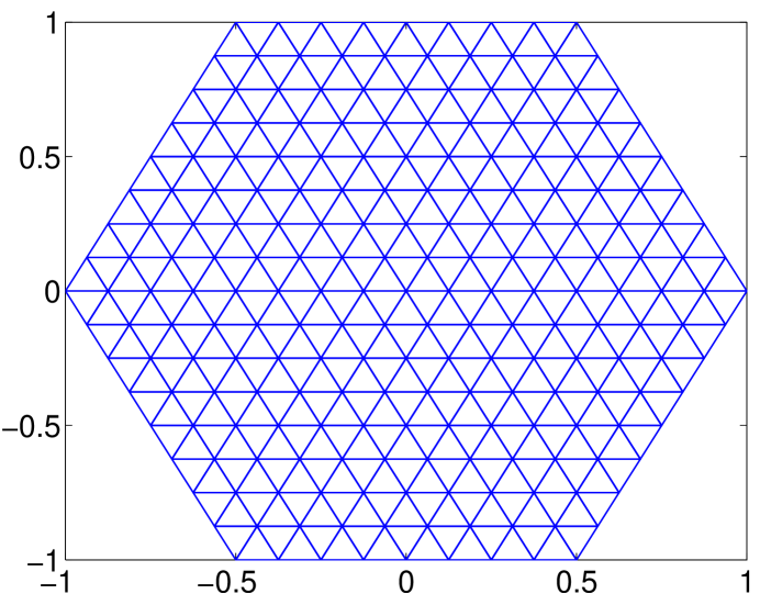
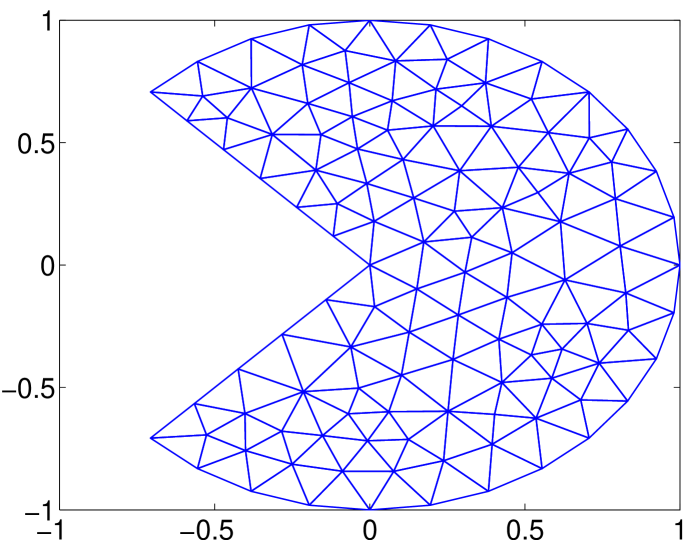
Fig. 1: Geometry of testing domains and sample meshes. Left: a convex hexagon domain; Right: a non-convex imperfect circular domain.

4.1 A convex Helmholtz problem

We first consider a homogeneous Helmholtz equation defined on a convex hexagon domain, which has been studied in [18]. The domain $\Omega$ is the unit regular hexagon domain centered at the origin $(0,0)$, see Fig. 1 (left). Here we set $d=1$ and $f=\sin(kr)/r$ in (1), where $r=\sqrt{x^{2}+y^{2}}$. The boundary data $g$ in the Robin boundary condition (2) is chosen so that the exact solution is given by

(13) $$u=\frac{\cos(kr)}{k}-\frac{\cos k+i\sin k}{k(J_{0}(k)+iJ_{1}(k))}J_{0}(kr)$$

where $J_{\xi}(z)$ are Bessel functions of the first kind. Let ${\mathcal{T}}_{h}$ denote the regular triangulation that consists of $6N^{2}$ triangles of size $h=1/N$, as shown in Fig. 1 (left) for $T_{\frac{1}{8}}$.

Table 1: Convergence of piecewise constant WG for the Helmholtz equation on a convex domain with wave number $k=1$.

	relative $H^{1}$		relative $L^{2}$
$h$	error	order	error	order
5.00e-01	2.49e-02		4.17e-03
2.50e-01	1.11e-02	1.16	1.05e-03	1.99
1.25e-01	5.38e-03	1.05	2.63e-04	2.00
6.25e-02	2.67e-03	1.01	6.58e-05	2.00
3.13e-02	1.33e-03	1.00	1.64e-05	2.00
1.56e-02	6.65e-04	1.00	4.11e-06	2.00

Table 1 illustrates the performance of the WG method with piecewise constant elements for the Helmholtz equation with wave number $k=1$. Uniform triangular partitions were used in the computation through successive mesh refinements. The relative errors in $L^{2}$ norm and $H^{1}$ semi-norm can be seen in Table 1. The Table also includes numerical estimates for the rate of convergence in each metric. It can be seen that the order of convergence in the relative $H^{1}$ semi-norm and relative $L^{2}$ norm are, respectively, one and two for piecewise constant elements.

Table 2: Convergence of piecewise linear WG for the Helmholtz equation on a convex domain with wave number $k=5$.

	relative $H^{1}$		relative $L^{2}$
$h$	error	order	error	order
2.50e-01	9.48e-03		2.58e-04
1.25e-01	2.31e-03	2.04	3.46e-05	2.90
6.25e-02	5.74e-04	2.01	4.47e-06	2.95
3.13e-02	1.43e-04	2.00	5.64e-07	2.99
1.56e-02	3.58e-05	2.00	7.06e-08	3.00
7.81e-03	8.96e-06	2.00	8.79e-09	3.01

High order of convergence can be achieved by using corresponding high order finite elements in the present WG framework. To demonstrate this phenomena, we consider the same Helmholtz problem with a slightly larger wave number $k=5$. The WG with piecewise linear functions was employed in the numerical approximation. The computational results are reported in Table 2. It is clear that the numerical experiment validates the theoretical estimates. More precisely, the rates of convergence in the relative $H^{1}$ semi-norm and relative $L^{2}$ norm are given by two and three, respectively.

4.2 A non-convex Helmholtz problem

We next explore the use of the WG method for solving a Helmholtz problem defined on a non-convex domain, see Fig. 1 (right). The medium is still assumed to be homogeneous, i.e., $d=1$ in (1). We are particularly interested in the performance of the WG method for dealing with the possible field singularity at the origin. For simplicity, only the piecewise constant $RT_{0}$ elements are tested for the present problem. Following [20], we take $f=0$ in (1) and the boundary condition is simply taken as a Dirichlet one: $u=g$ on $\partial\Omega$. Here $g$ is prescribed according to the exact solution [20]

(14) $$u=J_{\xi}(k\sqrt{x^{2}+y^{2}})\cos(\xi\arctan(y/x)).$$

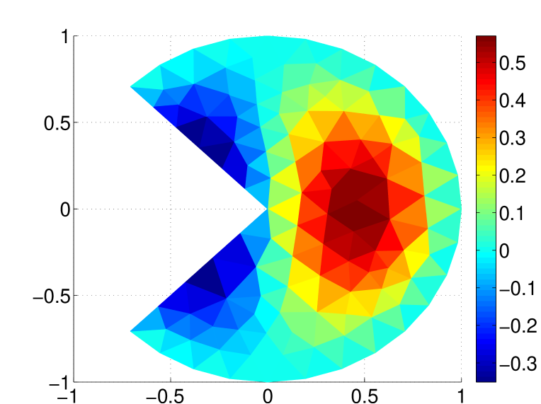
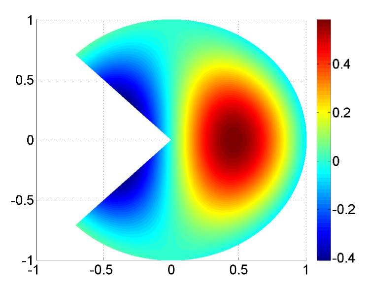
Fig. 2: WG solutions for the non-convex Helmholtz problem with $k=4$ and $\xi=1$. Left: Mesh level $1$; Right: Mesh level $6$.

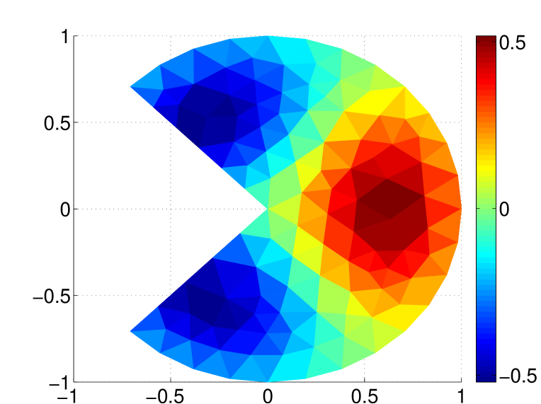
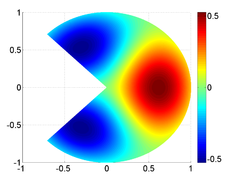
Fig. 3: WG solutions for the non-convex Helmholtz problem with $k=4$ and $\xi=3/2$. Left: Mesh level $1$; Right: Mesh level $6$.

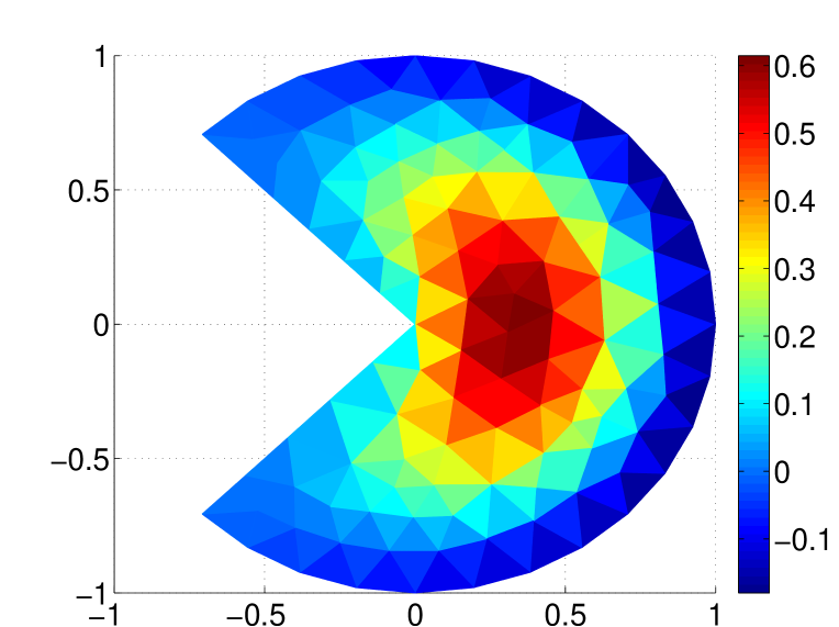
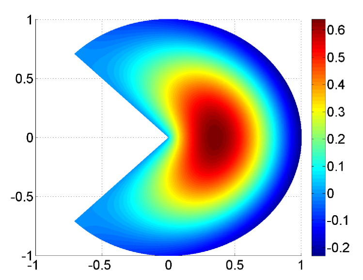
Fig. 4: WG solutions for the non-convex Helmholtz problem with $k=4$ and $\xi=2/3$. Left: Mesh level $1$; Right: Mesh level $6$.

In the present study, the wave number was chosen as $k=4$ and three values for the parameter $\xi$ are considered; i.e., $\xi=1$, $\xi=3/2$ and $\xi=2/3$. The same triangular mesh is used in the WG method for all three cases. In particular, an initial mesh is first generated by using MATLAB with default settings, see Fig. 1 (right). Next, the mesh is refined uniformly for five times. The WG solutions on mesh level $1$ and mesh level $6$ are shown in Fig. 2, Fig. 3, and Fig. 4, respectively, for $\xi=1$, $\xi=3/2$, and $\xi=2/3$. Since the numerical errors are quite small for the WG approximation corresponding to mesh level $6$, the field modes generated by the densest mesh are visually indistinguishable from the analytical ones. In other words, the results shown in the right charts of Fig. 2, Fig. 3, and Fig. 4 can be regarded as analytical results. It can be seen that in all three cases, the WG solutions already agree with the analytical ones at the coarsest level. Moreover, based on the coarsest mesh, the constant function values can be clearly seen in each triangle, due to the use of piecewise constant $RT_{0}$ elements. Nevertheless, after the initial mesh is refined for five times, the numerical plots shown in the right charts are very smooth. A perfect symmetry with respect to the $x$-axis is clearly seen.

Table 3: Numerical convergence test for the non-convex Helmholtz problem with $k=4$ and $\xi=1$.

	relative $H^{1}$		relative $L^{2}$
$h$	error	order	error	order
2.44e-01	5.64e-02		1.37e-02
1.22e-01	2.83e-02	1.00	3.56e-03	1.95
6.10e-02	1.42e-02	0.99	8.98e-04	1.99
3.05e-02	7.14e-03	1.00	2.25e-04	2.00
1.53e-02	3.57e-03	1.00	5.63e-05	2.00
7.63e-03	1.79e-03	1.00	1.41e-05	2.00

Table 4: Numerical convergence test for the non-convex Helmholtz problem with $k=4$ and $\xi=3/2$.

	relative $H^{1}$		relative $L^{2}$
$h$	error	order	error	order
2.44e-01	5.56e-02		1.12e-2
1.22e-01	2.81e-02	0.98	3.02e-03	1.89
6.10e-02	1.42e-02	0.99	8.06e-04	1.91
3.05e-02	7.14e-03	0.99	2.12e-04	1.92
1.53e-02	3.58e-03	1.00	5.54e-05	1.94
7.63e-03	1.79e-03	1.00	1.44e-05	1.95

Table 5: Numerical convergence test for the non-convex Helmholtz problem with $k=4$ and $\xi=2/3$.

	relative $H^{1}$		relative $L^{2}$
$h$	error	order	error	order
2.44e-01	1.07e-01		5.24e-02
1.22e-01	5.74e-02	0.90	2.18e-02	1.27
6.10e-02	3.23e-02	0.83	9.01e-03	1.27
3.05e-02	1.89e-02	0.77	3.68e-03	1.29
1.53e-02	1.14e-02	0.73	1.49e-03	1.31
7.63e-03	6.99e-03	0.71	5.96e-04	1.32

We next investigate the numerical convergence rates for WG. The numerical errors of the WG solutions for $\xi=1$, $\xi=3/2$ and $\xi=2/3$ are listed, respectively, in Table 3, Table 4, and Table 5. It can be seen that for $\xi=1$ and $\xi=3/2$, the numerical convergence rates in the relative $H^{1}$ and $L^{2}$ errors remain to be first and second order, while the convergence orders degrade for the non-smooth case $\xi=2/3$. Mathematically, for both $\xi=3/2$ and $\xi=2/3$, the exact solutions (14) are known to be non-smooth across the negative $x$-axis if the domain was chosen to be the entire circle. However, the present domain excludes the negative $x$-axis. Thus, the source term $f$ of the Helmholtz equation (1) can be simply defined as zero throughout $\Omega$. Nevertheless, there still exists some singularities at the origin $(0,0)$. In particular, it is remarked in [20] that the singularity lies in the derivatives of the exact solution at $(0,0)$. Due to such singularities, the convergence rates of high order discontinuous Galerkin methods are also reduced for $\xi=3/2$ and $\xi=2/3$ [20]. In the present study, we further note that there exists a subtle difference between two cases $\xi=3/2$ and $\xi=2/3$ at the origin. To see this, we neglect the second $\cos(\cdot)$ term in the exact solution (14) and plot the Bessel function of the first kind $J_{\xi}(k|r|)$ along the radial direction $r$, see Fig. 5. It is observed that the Bessel function of the first kind is non-smooth for the case $\xi=2/3$, while it looks smooth across the origin for the case $\xi=3/2$. Thus, it seems that the first derivative of $J_{3/2}(k|r|)$ is still continuous along the radial direction. This perhaps explains why the present WG method does not experience any order reduction for the case $\xi=3/2$. In [20], locally refined meshes were employed to resolve the singularity at the origin so that the convergence rate for the case $\xi=2/3$ can be improved. We note that local refinements can also be adopted in the WG method for a better convergence rate. A study of WG with grid local refinement is left to interested parties for future research.

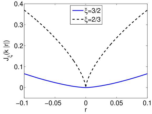
Fig. 5: The Bessel function of the first kind $J_{\xi}(k|r|)$ across the origin.

4.3 A Helmholtz problem with inhomogeneous media

We consider a Helmholtz problem with inhomogeneous media defined on a circular domain with radius $R$. Note that the spatial function $d(x,y)$ in the Helmholtz equation (1) represents the dielectric properties of the underlying media. In particular, we have $d=\frac{1}{\epsilon}$ in the electromagnetic applications [35], where $\epsilon$ is the electric permittivity. In the present study, we construct a smooth varying dielectric profile:

(15) $$d(r)=\frac{1}{\epsilon_{1}}S(r)+\frac{1}{\epsilon_{2}}(1-S(r)),$$

where $r=\sqrt{x^{2}+y^{2}}$, $\epsilon_{1}$ and $\epsilon_{2}$ are dielectric constants, and

(16) $$S(r)=\begin{cases}1&\text{if $r<a$},\\ -2\left(\frac{b-r}{b-a}\right)^{3}+3\left(\frac{b-r}{b-a}\right)^{2}&\text{if $a\leq r\leq b$},\\ 0&\text{if $r>b$},\end{cases}$$

with $a<b<R$. An example plot of $d(r)$ and $S(r)$ is shown in Fig. 6. In classical electromagnetic simulations, $\epsilon$ is usually taken as a piecewise constant, so that some sophisticated numerical treatments have to be conducted near the material interfaces to secure the overall accuracy [35]. Such a procedure can be bypassed if one considers a smeared dielectric profile, such as (15). We note that under the limit $b\to a$, a piecewise constant profile is recovered in (15). In general, the smeared profile (15) might be generated via numerical filtering, such as the so-called $\epsilon$-smoothing technique [30] in computational electromagnetics. On the other hand, we note that the dielectric profile might be defined to be smooth in certain applications. For example, in studying the solute-solvent interactions of electrostatic analysis, some mathematical models [11, 36] have been proposed to treat the boundary between the protein and its surrounding aqueous environment to be a smoothly varying one. In fact, the definition of (15) is inspired by a similar model in that field [11].

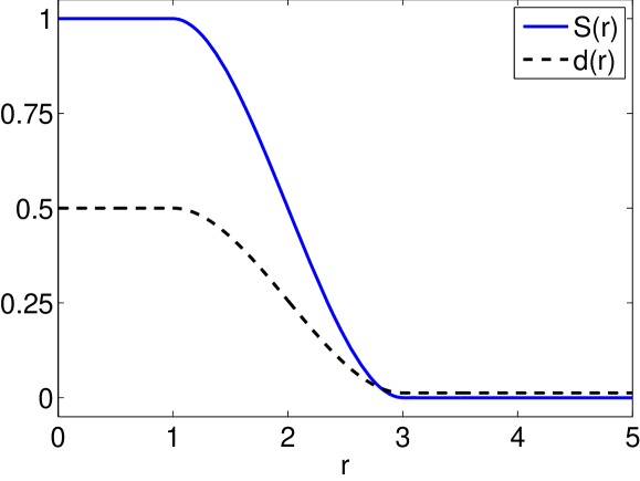
Fig. 6: An example plot of smooth dielectric profile $d(r)$ and $S(r)$ with $a=1$, $b=3$ and $R=5$. The dielectric coefficients of protein and water are used, i.e., $\epsilon_{1}=2$ and $\epsilon_{2}=80$.

In the present study, we choose the source of the Helmholtz equation (1) to be

(17) $$f(r)=\kappa^{2}[d(r)-1]J_{0}(kr)+kd^{\prime}(r)J_{1}(kr),$$

where

(18) $$d^{\prime}(r)=\left(\frac{1}{\epsilon_{1}}-\frac{1}{\epsilon_{2}}\right)S^{\prime}(r)$$

and

(19) $$S^{\prime}(r)=\begin{cases}0&\text{if $r<a$},\\ 6\left(\frac{b-r}{b-a}\right)^{2}-6\left(\frac{b-r}{b-a}\right)&\text{if $a\leq r\leq b$},\\ 0&\text{if $b<r$},\end{cases}$$

For simplicity, a Dirichlet boundary condition is imposed at $r=R$ with $u=g$. Here $g$ is prescribed according to the exact solution

(20) $$u=J_{0}(kr).$$

Our numerical investigation assumes the value of $a=1$, $b=3$ and $R=5$. The wave number is set to be $k=2$. The dielectric coefficients are chosen as $\epsilon_{1}=2$ and $\epsilon_{2}=80$, which represents the dielectric constant of protein and water [11, 36], respectively. The WG method with piecewise constant finite element functions is employed to solve the present problem with inhomogeneous media in Cartesian coordinate. Table 6 illustrates the computational errors and some numerical rate of convergence. It can be seen that the numerical convergence in the relative $L^{2}$ error is not uniform, while the relative $H^{1}$ error still converges uniformly in first order. This phenomena might be related to the non-uniformity and smallness of the media in part of the computational domain. In particular, we note that the relative $L^{2}$ error for the coarsest grid is extremely large, such that the numerical order for the first mesh refinement is unusually high. To be fair, we thus exclude this data in our analysis. To have an idea about the overall numerical order of this non-uniform convergence, we calculated the average convergence rate and least-square fitted convergence rate for the rest mesh refinements, which are $1.97$ and $1.88$, respectively. Thus, the present inhomogeneous example demonstrates the accuracy and robustness of the WG method for the Helmholtz equation.

Table 6: Numerical convergence test of the Helmholtz equation with inhomogeneous media.

	relative $H^{1}$		relative $L^{2}$
$h$	error	order	error	order
1.51e-00	2.20e-01		1.04e-00
7.54e-01	1.24e-01	0.83	1.20e-01	3.11
3.77e-01	6.24e-02	0.99	1.81e-02	2.73
1.88e-01	3.13e-02	1.00	5.71e-03	1.67
9.42e-02	1.56e-02	1.00	2.14e-03	1.42
4.71e-02	7.82e-03	1.00	5.11e-04	2.06

4.4 Large wave numbers

We finally investigate the performance of the WG method for the Helmholtz equation with large wave numbers. As discussed above, without resorting to high order generalizations or analytical/special treatments, we will examine the use of the plain WG method for tackling the pollution effect. The homogeneous Helmholtz problem of the Subsection 4.1 will be studied again. Also, the $RT_{0}$ and $RT_{1}$ elements are used to solve the homogeneous Helmholtz equation with the Robin boundary condition. Since this problem is defined on a structured hexagon domain, a uniform triangular mesh with a constant mesh size $h$ throughout the domain is used. This enables us to precisely evaluate the impact of the mesh refinements. Following the literature works [6, 18], we will focus only on the relative $H^{1}$ semi-norm in the present study.

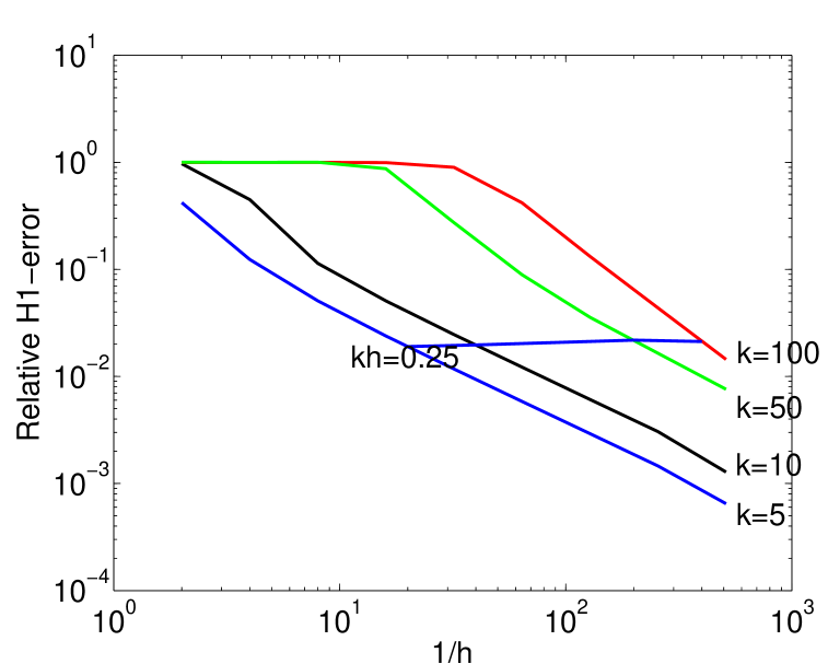
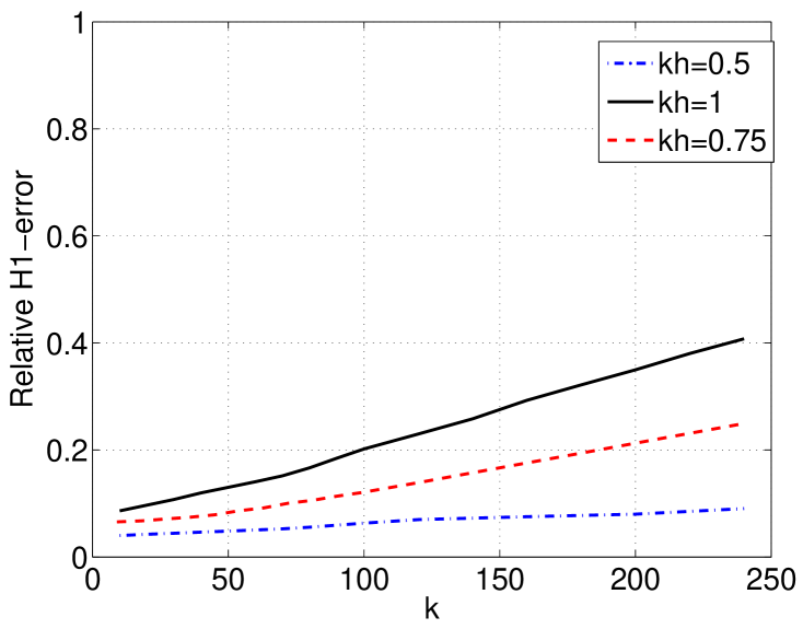
Fig. 7: Relative $H^{1}$ error of the WG solution. Left: with respect to $1/h$; Right: with respect to wave number $k$.

To study the non-robustness behavior with respect to the wave number $k$, i.e., the pollution effect, we solve the corresponding Helmholtz equation by using piecewise constant WG method with various mesh sizes for four wave numbers $k=5$, $k=10$, $k=50$, and $k=100$, see Fig. 7 (left) for the WG performance. From Fig. 7 (left), it can be seen that when $h$ is smaller, the WG method immediately begins to converge for the cases $k=5$ and $k=10$. However, for large wave numbers $k=50$ and $k=100$, the relative error remains to be about $100$%, until $h$ becomes to be quite small or $1/h$ is large. This indicates the presence of the pollution effect which is inevitable in any finite element method [5]. In the same figure, we also show the errors of different $k$ values by fixing $kh=0.25$. Surprisingly, we found that the relative $H^{1}$ error does not evidently increase as $k$ becomes larger. The convergence line for $kh=0.25$ looks almost flat, with a very little slope. In other words, the pollution error is very small in the present WG result. We note that such a result is as good as the one reported in [18] by using a penalized discontinuous Galerkin approach with optimized parameter values. In contrast, no parameters are involved in the WG scheme.

On the other hand, the good performance of the WG method for the case $kh=0.25$ does not mean that the WG method could be free of pollution effect. In fact, it is known theoretically [5] that the pollution error cannot be eliminated completely in two- and higher-dimensional spaces for Galerkin finite element methods. In the right chart of Fig. 7, we examine the numerical errors by increasing $k$, under the constraint that $kh$ is a constant. Huge wave numbers, up to $k=240$, are tested. It can be seen that when the constant changes from $0.5$ to $0.75$ and $1.0$, the non-robustness behavior against $k$ becomes more and more evident. However, the slopes of $kh$=constant lines remain to be small and the increment pattern with respect to $k$ is always monotonic. This suggests that the pollution error is well controlled in the WG solution.

Fig. 8: Exact solution (left) and piecewise constant WG approximation (right) for $k=100,$ and $h=1/60.$

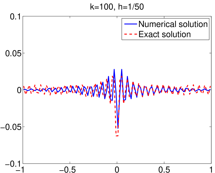
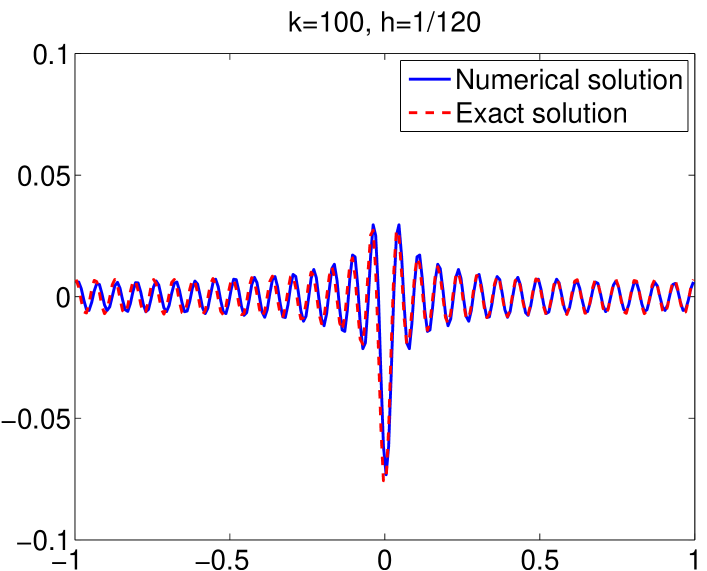
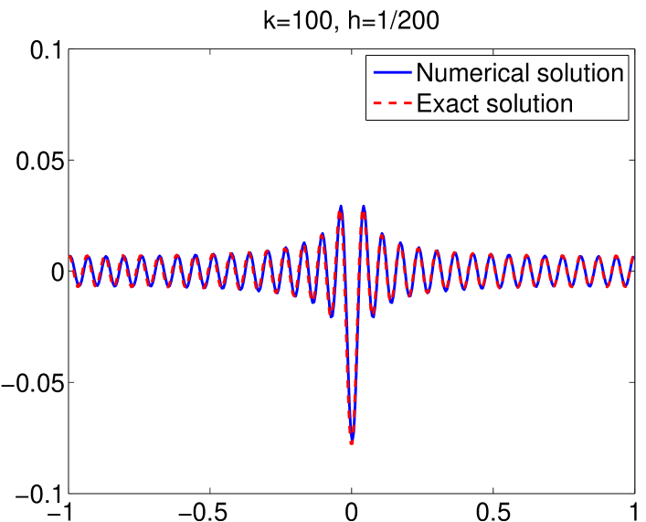
Fig. 9: The trace plot along $x$-axis or $y=0$ form WG solution using piecewise constants.

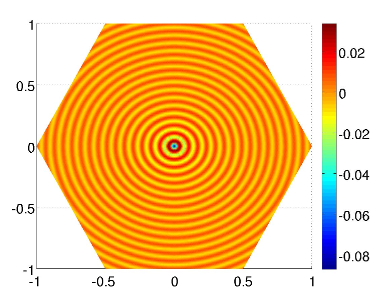
Fig. 10: Exact solution (left) and piecewise linear WG approximation (right) for $k=100,$ and $h=1/60.$

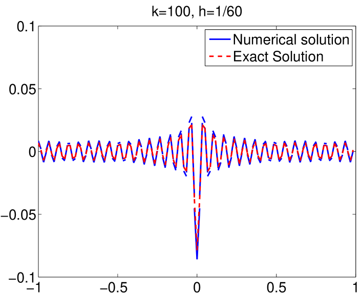
Fig. 11: The trace plot along $x$-axis or $y=0$ form WG solution using piecewise linear elements.

In the rest of the paper, we shall present some numerical results for the WG method when applied to a challenging case of high wave numbers. In Fig. 8 and 10, the WG numerical solutions are plotted against the exact solution of the Helmholtz problem. Here we take a wave number $k=100$ and mesh size $h=1/60$ which is relatively a coarse mesh. With such a coarse mesh, the WG method can still capture the fast oscillation of the solution. However, the numerically predicted magnitude of the oscillation is slightly damped for waves away from the center when piecewise constant elements are employed in the WG method. Such damping can be seen in a trace plot along $x$-axis or $y=0$. To see this, we consider an even worse case with $k=100$ and $h=1/50$. The result is shown in the first chart of Fig. 9. We note that the numerical solution is excellent around the center of the region, but it gets worse as one moves closer to the boundary. If we choose a smaller mesh size $h=1/120$, the visual difference between the exact and WG solutions becomes very small, as illustrate in Fig. 9. If we further choose a mesh size $h=1/200$, the exact solution and the WG approximation look very close to each other. This indicates an excellent convergence of the WG method when the mesh is refined. In addition to mesh refinement, one may also obtain a fast convergence by using high order elements in the WG method. Figure 11 illustrates a trace plot for the case of $k=100$ and $h=1/60$ when piecewise linear elements are employed in the WG method. It can be seen that the computational result with this relatively coarse mesh captures both the fast oscillation and the magnitude of the exact solution very well.

5 Concluding Remarks

The present numerical experiments indicate that the WG method as introduced in [33] is a very promising numerical technique for solving the Helmholtz equations with large wave numbers. This finite element method is robust, efficient, and easy to implement. On the other hand, a theoretical investigation for the WG method should be conducted by taking into account some useful features of the Helmholtz equation when special test functions are used. It would also be valuable to test the performance of the WG method when high order finite elements are employed to the Helmholtz equations with large wave numbers in two and three dimensional spaces.

Finally, it is appropriate to clarify some differences and connections between the WG method and other discontinuous finite element methods for solving the Helmholtz equation. Discontinuous functions are used to approximate the Helmholtz equation in many other finite element methods such as discontinuous Galerkin (DG) methods [18, 3, 12] and hybrid discontinuous Galerkin (HDG) methods [14, 15, 20].

However, the WG method and the HDG method are fundamentally different in concept and formulation. The HDG method is formulated by using the standard mixed method approach for the usual system of first order equations, while the key to the WG is the use of the discrete weak differential operators. For a second order elliptic problem, these two methods share the same feature by approximating first order derivatives or fluxes through a formula that was commonly employed in the mixed finite element method. For high order partial differential equations (PDEs), the WG method is greatly different from the HDG. Consider the biharmonic equation [29] as an example. The first step of the HDG formulation is to rewrite the fourth order equation to four first order equations. In contrast, the WG formulation for the biharmonic equation can be derived directly from the variational form of the biharmonic equation by replacing the Laplacian operator $\Delta$ by a weak Laplacian $\Delta_{w}$ and adding a parameter free stabilizer [29]. It should be emphasized that the concept of weak derivatives makes the WG a widely applicable numerical technique for a large variety of PDEs which we shall report in forthcoming papers.

For the Helmholtz equation studied in this paper, the WG method and the HDG method yield the same variational form for the homogeneous Helmholtz equation with a constant $d$ in (1). However, the WG discretization differs from the HDG discretization for an inhomogeneous media problem with $d$ being a spatial function of $x$ and $y$. Moreover, the WG method has an advantage over the HDG method when the coefficient $d$ is degenerated.

References

- [1] M. Ainsworth, Discrete dispersion relation for hp-version finite element approximation at high wave number, SIAM J. Numer. Anal., 42, pp. 553-575, 2004.
- [2] M. Ainsworth and H.A. Wajid, Dispersive and dissipative behavior of the spectral element method, SIAM J. Numer. Anal., 47, pp. 3910-3937, 2009.
- [3] D. Arnold, F. Brezzi, B. Cockburn, and L. D. Marini, Unified analysis of discontinuous Galerkin methods for elliptic problems, SIAM J. Numer. Anal., 39 (2002), pp. 1749–1779.
- [4] I. Babuška, F. Ihlenburg, E.T. Paik, S.A. Sauter, A generalized finite element method for solving the Helmholtz equation in two dimensions with minimal pollution. Computer Methods in Applied Mechanics and Engineering 1995; 128: 325-359.
- [5] I. Babuška, S.A. Sauter, Is the pollution effect of the FEM avoidable for the Helmholtz equation considering high wave number? SIAM Journal on Numerical Analysis 1997; 34: 2392-2423. Reprinted in SIAM Review 2000; 42: 451-484.
- [6] G. Bao, G.W. Wei, and S. Zhao, Numerical solution of the Helmholtz equation with high wavenubers, Int. J. Numer. Meth. Engng, 59 (2004), pp. 389-408.
- [7] F. Brezzi and M. Fortin, Mixed and Hybrid Finite Elements, Springer-Verlag, New York, 1991.
- [8] O. Cessenat and B. Despres, Application of the ultra-weak variational formulation of elliptic PDEs to the 2-dimensional Helmholtz problem, SIAM J. Numer. Anal., 35 (1998), pp. 255-299.
- [9] O. Cessenat and B. Despres, Using plane waves as base functions for solving time harmonic equations with the ultra weak varational formulation, J. Comput. Acoustics, 11 (2003), pp. 227-238.
- [10] S.N. Chandler-Wilde and S. Langdon, A Galerkin boundary element method for high frequency scattering by convex polygons, SIAM J. Numer. Anal., 45 (2007), pp. 610-640.
- [11] Z. Chen, N.A. Baker, and G.W. Wei, Differential geometry based solvation model I: Eulerian formulation, J. Comput. Phys., 229 (2010), pp. 8231-8258.
- [12] E.T. Chung and B. Engquist, Optimal discontinuous Galerkin methods for wave propagation, SIAM J. Numer. Anal., 44 (2006), pp. 2131-2158.
- [13] P.G. Ciarlet, The Finite Element Method for Elliptic Problems, North-Holland, New York, 1978.
- [14] B. Cockburn, B. Dong, and J. Guzman, A superconvergent LDG-hybridizable Galerkin method for second-order elliptic problems, Math. COmput. 77 (2008), pp. 1887-1916.
- [15] B. Cockburn, J. Gopalakrishnan, and R. Lazarov, Unified hybridization of discontinuous Galerkin, mixed and continuous Galerkin methods for second- order elliptic problems, SIAM J. Numer. Anal. 47 (2009), pp. 1319-1365.
- [16] C. Harhat, I. Harari, and U. Hetmaniuk, A discontinuous Galerkin methodwith Lagrange multiplies for the solution of Helmholtz problems in the mid-frequency regime, Comput. Methods Appl. Mech. Engrg., 192 (2003), pp. 1389-1419.
- [17] C. Harhat, R. Tezaur, and P. Weidemann-Goiran, Higher-order extensions of a discontinuous Galerkin method for mid-frequency Helmholtz problems, Int. J. Numer. Meth. Engng, 61 (2004), pp. 1938-1956.
- [18] X. Feng and H. Wu, Discontinuous Galerkin methods for the Helmholtz equation with large wave number, SIAM J. Numer. Anal., 47 (2009), pp. 2872-2896.
- [19] E. Giladi, Asymptotically derived boundary elements for the Helmholtz equation in high frequencies, J. Comput. Appl. Math. 2007; 198, 52-74.
- [20] R. Griesmaier and P. Monk, Error analysis for a hybridizable discontinuous Galerkin method for the Helmholtz equation, J. Sci. Comput. 2011; 49, 291-310.
- [21] E. Heikkola, S. Monkola, A. Pennanen, and T. Rossi, Controllability method for the Helmholtz equation with higher-order discretizations. J. Comput. Phys. 2007; 225: 1553-1576.
- [22] F. Ihlenburg, I. Babuška, Dispersion analysis and error estimation of Galerkin finite element methods for the Helmholtz equation. International Journal for Numerical Methods in Engineering 1995; 38: 3745-3774.
- [23] F. Ihlenburg, I. Babuška, Finite element solution of the Helmholtz equation with high wavenumber Part I: the -version of the FEM. Computer and Mathematics with applications 1995; 30: 9-37.
- [24] F. Ihlenburg, I. Babuška, Finite element solution of the Helmholtz equation with high wavenumber Part II: the --version of the FEM. SIAM Journal of Numerical Analysis 1997; 34: 315-358.
- [25] S. Langdon and S.N. Chandler-Wilde, A wavenumber independent boundary element method for an accoustic scattering problem, SIAM J. Numer. Anal., 43 (2006), pp. 2450-2477.
- [26] J.M. Melenk and I. Babuška, The partition of unity finite element method: Basic theory and applications, Comput. Methods Appl. Mech. Engrg. 139, (1996), pp. 289-314.
- [27] P. Monk and D.Q. Wang, A least-squares method for the Helmholtz equation, Comput. Methods Appl. Mech. Engrg. 175, (1999), pp. 121-136.
- [28] L. Mu, J. Wang, and X. Ye, A Weak Galerkin Finite Element Method with Polynomial Reduction, 2013. Availabe at: (arXiv:1304.6481).
- [29] L. Mu, J. Wang, and X. Ye, Weak Galerkin Finite Element Methods for the Biharmonic Equation on Polytopal Meshes, 2013. Available at: (arXiv:1303.0927).
- [30] Z.H. Shao, G.W. Wei and S. Zhao, DSC time-domain solution of Maxwell’s equations, J. Comput. Phys., 189 (2003), pp. 427-453.
- [31] J. Shen and L.-L. Wang, Spectral approximation of the Helmholtz equation with high wave numbers, SIAM J. Numer. Anal., 43 (2005), pp. 623-644.
- [32] J. Shen and L.-L. Wang, Analysis of a spectral-Galerkin approximation to the Helmhotlz equation in exterior domains, SIAM J. Numer. Anal., 45 (2007), pp. 1954-1978.
- [33] J. Wang and X. Ye, A weak Galerkin finite element method for second-order elliptic problems, J. Comp. and Appl. Math, 241 (2013) 103-115.
- [34] J. Wang and X. Ye, A Weak Galerkin mixed finite element method for second-order elliptic problems, Math. Comp., to appear, (2013). Available at: (arXiv:1202.3655).
- [35] S. Zhao, High order matched interface and boundary methods for the Helmholtz equation in media with arbitrarily curved interfaces, J. Comput. Phys., 229 (2010), pp. 3155-3170.
- [36] S. Zhao, Pseudo-time coupled nonlinear models for biomolecular surface representation and solvation analysis, Int. J. Numer. Methods Biomedical Engrg., 27 (2011), 1964-1981.
- [37] O.C. Zienkiewicz, Achievements and some unsolved problems of the finite element method. International Journal for Numerical Methods in Engineering 2000; 47: 9-28.