Abstract

Three-dimensional $Z(N)$ lattice gauge theories at zero temperature are studied for various values of $N$. Using a modified phenomenological renormalization group, we explore the critical behavior of the generalized $Z(N)$ model for $N=2,3,4,5,6,8$. Numerical computations are used to simulate vector models for $N=2,3,4,5,6,8,13,20$ for lattices with linear extension up to $L=96$. We locate the critical points of phase transitions and establish their scaling with $N$. The values of the critical indices indicate that the models with $N>4$ belong to the universality class of the three-dimensional $XY$ model. However, the exponent $\alpha$ derived from the heat capacity is consistent with the Ising universality class. We discuss a possible resolution of this puzzle. We also demonstrate the existence of a rotationally symmetric region within the ordered phase for all $N\geq 5$ at least in the finite volume.

  e-mail addresses:

^†oleg@bitp.kiev.ua,   ^∗chelnokov@bitp.kiev.ua,   ^††cortese@unizar.es,

^‡gravina@cs.infn.it,   ^¶papa@cs.infn.it,   ^∗∗i_van_go@inbox.ru

1 Introduction

Models possessing global and/or local discrete $Z(N)$ symmetry play an important role in many branches of physics ranging from the solid state physics to the description of the universality features of the deconfining transition in $SU(N)$ gauge theories. In this paper we are interested in the $Z(N)$ lattice gauge theory (LGT) at zero temperature. Assigning the gauge fields $s_{n}(x)=0,1,\cdots,N-1$ to the links of a simple hypercubic lattice, the most general action of the isotropic $Z(N)$ LGT can be written as

$$S_{\rm gauge}=\frac{1}{2}\ \sum_{x}\sum_{n<m}\ \sum_{k=1}^{N-1}\beta_{k}\exp\left(\frac{2\pi ik}{N}\left(s_{n}(x)+s_{m}(x+e_{n})-s_{n}(x+e_{m})-s_{m}(x)\right)\right)\ ,$$ (1)

where $e_{n}$, $n=1,2,3$, denotes the unit vector in the $n$-th direction. Similarly, the most general action of the $Z(N)$ spin model is given by

$$S_{\rm spin}\ =\ \frac{1}{2}\ \sum_{x}\sum_{n}\ \sum_{k=1}^{N-1}\beta_{k}\exp\left(\frac{2\pi ik}{N}\left(s(x)-s(x+e_{n})\right)\right)\ .$$ (2)

In both cases we used the convention

$$\beta_{k}\ =\ \beta_{-k}\ =\ \beta_{k+N}\ >\ 0\ .$$ (3)

The standard Potts model corresponds to the choice when all $\beta_{k}$ are equal. Then, the sum over $k$ reduces to a delta-function on the $Z(N)$ group. The conventional vector model corresponds to $\beta_{k}=0$ for all $k\neq 1,N-1$. For $N=2,3$ the Potts and vector models are equivalent.

Two-dimensional (2D) standard and vector $Z(N)$ LGTs are exactly solvable both in the finite volume and in the thermodynamic limit. They exhibit no phase transition at any finite value of the coupling constant $\beta$. In particular, the rectangular $R\times T$ Wilson loop in the representation $k$ obeys the area law

$$\langle W_{k}(S)\rangle\ =\ \exp\left(-\sigma_{k}(N)\ R\ T\right)\ ,$$

thus implying a permanent confinement of static charges. For example, the string tension of the vector model in the thermodynamic limit reads

$$\sigma_{k}(N)\ =\ \ln\left[\frac{C_{0}(N,\beta)}{C_{k}(N,\beta)}\right]\ >0\ \ ,\ \ C_{k}(N,\beta)\ =\ \sum_{r=-\infty}^{\infty}\ I_{Nr+k}(\beta)\ .$$

Here, $I_{k}(x)$ is the modified Bessel function.

No exact solution has been found for any $Z(N)$ model in $3D$, where the phase structure becomes highly non-trivial. While the phase structure of the general model defined by (1) remains unknown, it is well established that Potts models and vector models with only $\beta_{1}$ non-vanishing have one phase transition from a confining phase to a phase with vanishing string tension [1, 2, 3]. Via duality, $Z(N)$ gauge models can be exactly related to $3D$ $Z(N)$ spin models. In particular, a Potts gauge theory is mapped to a Potts spin model, and such a relation allows to establish the order of the phase transition. Hence, Potts LGTs with $N=2$ have second order phase transition, while for $N\geq 3$ one finds a first order phase transition. Since $Z(2)$ LGT is equivalent to the Ising model, its critical behavior is well known (see Refs. [4] and references therein). Generally, the $Z(N)$ global symmetry of the finite-temperature $4D$ $SU(N)$ gauge theory motivated thorough investigations, both analytical and numerical, of the $3D$ spin models, especially for $N=2,3$ [5, 6] (for more recent studies, see [7] and references therein). The $3D$ Potts models for $N>3$ have been simulated in [8] and studied by means of the high-temperature expansion in [9].

Surprisingly, much less is known about the critical behavior of $Z(N)$ vector LGTs when $N>4$. They have been studied numerically in [10] up to $N=20$ on symmetric lattices with size $L\in[4-16]$. It was confirmed that zero-temperature models possess a single phase transition which disappears in the limit $N\to\infty$. A scaling formula proposed in [10] shows that the critical coupling diverges like $N^{2}$ for large $N$. Thus, the $U(1)$ LGT has a single confined phase in agreement with theoretical results [11]. We are not aware, however, of any detailed study of the critical behavior of the vector models with $N\geq 4$ in the vicinity of this single phase transition. Slightly more is known about the critical properties of $Z(N)$ vector spin models. In particular, it has been suggested that all vector spin models exhibit a single second order phase transition [12]. An especially detailed study was performed on the $Z(6)$ model, because the $Z(6)$ global symmetry appears as an effective symmetry of the $Z(3)$ antiferromagnetic Potts model [13, 14]. The computed critical indices suggest that the $Z(6)$ vector model belongs to the universality class of the $3D$ $XY$ model. An interesting feature of the $Z(6)$ model and, possibly, of all vector models with $N>4$, is the appearance of an intermediate rotationally symmetric region below the critical temperature of the second order phase transition. The mass gap was however found to be rather small, but non-vanishing in this region [13]. Combined with a renormalization group (RG) study, the analysis concluded that this intermediate region presents a crossover to a low-temperature massive phase, where the discreteness of $Z(6)$ plays an essential role [14].

The main goal of the present work is to fill the gap in our knowledge about the critical behavior of the $3D$ $Z(N)$ LGTs. Another motivation comes from our recent studies of the deconfinement transition in the $Z(N)$ vector LGT for $N>4$ at finite temperatures [15, 16, 17]. The major findings of these papers was the demonstration of two phase transitions of the Berezinskii-Kosterlitz-Thouless type and the existence of an intermediate massless phase. The critical indices at these transitions have been found to coincide with the indices of the $2D$ vector spin models. An interesting question then arises regarding the construction of the continuum limit of the finite-temperature models in the vicinity of the critical points. For this to accomplish it might be useful, and even necessary, to know the scaling of quantities such as string tension, correlation length, etc. near the critical points of the corresponding zero temperature models.

In this work we are going to:

• perform an analytical study of the general $3D$ $Z(N)$ LGT for various $N$ using a “phenomenological” RG;

• locate critical points of the vector models via Monte Carlo simulations of the dual of the $Z(N)$ LGT and determine their scaling with $N$;

• compute some critical indices and establish the universality class of the models;

• illustrate the existence of a rotationally symmetric region within the ordered phase for all $N\geq 5$ at least in the finite volume.

This paper is organized as follows. In Section 2 we formulate our model and recall the exact duality relation with a generalized $3D$ $Z(N)$ spin model. Section 3 is devoted to a RG study of the models. Within a modified version of the phenomenological RG, we explore the space of coupling constants, find fixed points and calculate the critical index $\nu$. In Section 4 we present the setup of Monte Carlo simulations, define the observables used in this work and present the numerical results. In particular, we locate the position of critical points and compute various critical indices at these points. As a cross-check, we also simulated $Z(N=2,3)$ models for which high-precision results. The same Section deals also with the computation of the average action and the heat capacity in the vicinity of critical points and the derivation of the index $\alpha$ from a finite size scaling (FSS) analysis of the heat capacity. In Section 5 we discuss some findings regarding the symmetric region below the critical point. All results are finally summarized in Section 6.

2 Relation of the $3D$ $Z(N)$ LGT to a generalized $3D$ $Z(N)$ spin model

We work on a $3D$ lattice $\Lambda=L^{3}$ with linear extension $L$; $\vec{x}=(x_{1},x_{2},x_{3})$, where $x_{i}\in[0,L-1]$ denote the sites of the lattice and $e_{n}$, $n=1,2,3$, denotes the unit vector in the $n$-th direction. Periodic boundary conditions (BC) on gauge fields are imposed in all directions. We introduce conventional plaquette angles $s(p)$ as

$$s(p)\ =\ s_{n}(x)+s_{m}(x+e_{n})-s_{n}(x+e_{m})-s_{m}(x)\ .$$ (4)

The $3D$ $Z(N)$ LGT on an isotropic lattice can generally be defined as

$$Z(\Lambda;\{\beta_{k}\};N)\ =\ \prod_{l\in\Lambda}\left(\frac{1}{N}\sum_{s(l)=0}^{N-1}\right)\ \prod_{p}Q(s(p))\ .$$ (5)

The most general $Z(N)$-invariant Boltzmann weight is

$$Q(s)\ =\ \exp\left[\frac{1}{2}\sum_{k=1}^{N-1}\beta_{k}\exp\left(\frac{2\pi ik}{N}s\right)\right]\ .$$ (6)

The $U(1)$ LGT is defined as the limit $N\to\infty$ of the above expressions.

To study the phase structure of $3D$ $Z(N)$ LGTs one can map the gauge model to a generalized $3D$ $Z(N)$ spin model with the action given by Eq. (2). The relation between spin $\beta_{k}^{s}$ and gauge $\beta_{k}^{g}$ couplings can be computed exactly and reads

$$\beta_{k}^{s}\ =\ \frac{1}{N}\sum_{p=0}^{N-1}\ln\left[\frac{Q_{d}(p)}{Q_{d}(0)}\right]\ \cos\left(\frac{2\pi pk}{N}\right)\ ,$$ (7)

where the dual Boltzmann weight is defined as

$$Q_{d}(s)\ =\ \sum_{p=0}^{N-1}\ Q(p)\ \cos\left(\frac{2\pi ps}{N}\right)\ .$$ (8)

In what follows we are going to simulate the $Z(N)$ vector LGT. In this case we use $\beta_{1}=\beta_{N-1}=\beta$ and the dual weight becomes

$$Q_{d}(s)\ =\ \sum_{r=-\infty}^{\infty}\ I_{Nr+s}(\beta)\ .$$ (9)

An example of the explicit relations between couplings in this case together with some further important comments on the relations can be found in [17].

With the goal of performing RG transformations, it is somewhat more convenient to use a different but equivalent representation for the Boltzmann weight, namely

$$Q\left[\{t_{k}\};s\right]\ =\ \sum_{k=0}^{N-1}\ t_{k}\ \exp\left[\frac{2\pi i}{N}\ k\ s\right]\ .$$ (10)

The set of coupling constants $\{t_{k}\}$ can be chosen to satisfy

$$t_{0}=1\ ,\ 0\leq t_{k}\leq 1\ ,\ t_{k}=t_{-k}=t_{k+N}\ .$$

The coupling constants $t_{k}$ and $\beta_{k}$ can be connected to each other via the Fourier transform on the $Z(N)$ group. The dual of the partition function (5) can then be presented as

$$Z(\Lambda;\{t_{k}\};N)\ =\ \sum_{j_{n}=0}^{N-1}\ \prod_{x\in\Lambda}\ \left(\frac{1}{N}\sum_{s(x)=0}^{N-1}\right)\ \prod_{x,n}\ t_{s(x)-s(x+e_{n})+\eta_{n}}\ .$$ (11)

Here, the summations over $j_{n},n=1,2,3$, enforce the global Bianchi constraints due to the periodic BC and $\eta_{n}=j_{n}$ on a set of links dual to any fixed closed surface wrapping the original lattice in the directions perpendicular to $n$, otherwise $\eta_{n}=0$.

3 Results of the RG study

As a first step we consider the general $3D$ $Z(N)$ LGT with the Boltzmann weight (10) and study its phase structure with the help of the phenomenological renormalization group (PH RG) [18]. For the $3D$ Ising model this RG was used in [19]. As is well known, the PH RG gives in many cases not only the qualitatively correct phase diagram of a model, but also a good quantitative approximation for the observables near the critical points, and this approximation can be systematically improved. We follow the general strategy described in the original papers [18] and only briefly outline our modifications (for a detailed account of these modifications, together with application to other models, see [20]). As is common for this type of RG, we preserve the mass gap during the RG steps. We proceed as follows.

1. As a starting point we always use the dual formulations, i.e. Eq. (11) in the present case.

2. As a simplest $3D$ strip, we take a lattice $\Lambda_{s}=(2\times 2\times L)$ with periodic BC in both transverse directions and periodic or free BC in the longitudinal direction. Correlation functions are computed on $\Lambda_{s}$ and on a one-dimensional lattice for all representations.

3. The requirement of mass gap preservation leads to equations for the fixed points

   $$t_{j}^{(1)}\ =\ \left[\frac{\lambda_{j}(\{t_{k}\})}{\lambda_{0}(\{t_{k}\})}\right]^{2}\ ,$$ (12)

   where $\lambda_{j}(\{t_{k}\})$ is the eigenvalue of the transfer matrix corresponding to the correlation function in the representation $j$. This set of equations is treated as the recursion relations for the renormalized coupling constants.

4. The summation over the spins lying in one plane perpendicular to the longitudinal direction introduces all possible interactions between the remaining spins. The transfer matrix is constructed for the evolution of all independent couplings of this general interaction. This substantially reduces the size of the matrix.

5. Combining the PH RG in the form described above with the cluster decimation approximation of Ref. [21], we can construct new partition and correlation functions on a decimated lattice with double lattice spacing. The next iteration is performed with newly computed constants $t_{j}^{(1)}$.

In the framework of this approach we have explored the phase structure of the generalized $Z(N)$ model. Only in the case of the standard Potts model we can restrict ourselves to one iteration, since the RG steps do not generate new interactions. For the general case one should perform many iterations to locate precisely the critical points. The critical indices are calculated in the fixed point of the iterations where the critical points of the models of a given universality class are flowing to. Thorough discussion of the general case will be given in [20]. Here we report on the results for the vector LGTs relevant for this paper.

Table 1: $3D$ $Z(N)$ standard Potts models: $\beta_{\rm c}$ from the PH RG (column two) and from the Monte Carlo simulations of Ref. [8] (column three).
$3D$ $Z(N)$ vector models: $\beta_{\rm c}$ from the PH RG (column 4) and from the Monte Carlo simulations of this work (column five); critical index $\nu$ from the PH RG.

	Potts model		Vector model
$N$	$\beta_{\rm c}$	$\beta_{\rm c}^{\rm MC}$	$\beta_{\rm c}$	$\beta_{\rm c}^{\rm MC}$	$\nu$
2	0.77706	0.761414(2)	0.77706	0.761395(4)	0.616656
3	1.17186	1.084314(8)	1.17186	1.0844(2)	-
4	1.34363	1.288239(5)	1.55411	1.52276(4)	0.616657
5	1.50331	1.438361(4)	2.17896	2.17961(10)	0.692226
6	1.62881	1.557385(4)	2.99296	3.00683(7)	0.699208
8	1.81941	1.740360(6)	5.09472	5.12829(13)	0.699583
13	-	-	-	13.1077(3)	-
20	-	-	-	30.6729(5)	-

In Table 1 we present the estimates of the critical points $\beta_{\rm c}$, both in standard Potts models and in vector models, coming from the PH RG, and compare them with the results of Monte Carlo numerical simulations. In the case of standard Potts models, these simulations were performed in Ref. [8], while for the vector models, they were carried out in this paper. One can see that the PH RG based on the smallest possible strip and combined with the cluster decimation approximation gives quite accurate predictions both for the critical coupling and, as we will see later on, also for the index $\nu$.

4 Numerical results

4.1 Setup of the Monte Carlo simulation

The model under exam in this work is described by the action given in Eqs. (5) and (6), with couplings $\beta_{1}=\beta_{N-1}\equiv\beta$, $\beta_{n}=0$, $n=2,\ldots,N-2$. To study the phase transitions it turns out to be more convenient to simulate the dual spin model, whose action is given in (2) with the coupling constants computed according to Eq. (7). Simulations were performed by means of a cluster algorithm on symmetric lattices $L^{3}$ with periodic BC and $L$ in the range 8 – 96. For each Monte Carlo run the typical number of generated configurations was $2.5\cdot 10^{6}$, the first $10^{5}$ of them being discarded to ensure thermalization. Measurements were taken after every 10 updatings and error bars were estimated by the jackknife method combined with binning.

We considered the following observables:

• complex magnetization $M_{L}=|M_{L}|e^{i\psi}$,

  $$M_{L}\ =\ \sum_{x\in\Lambda}\exp\left(\frac{2\pi i}{N}s(x)\right)\;;$$ (13)

• population $S_{L}$,

  $$S_{L}\ =\ \frac{N}{N-1}\left(\frac{\max_{i=0,N-1}n_{i}}{L^{3}}-\frac{1}{N}\right)\;,$$ (14)

  where $n_{i}$ is number of $s(x)$ equal to $i$;

• real part of the rotated magnetization $M_{R}=|M_{L}|\cos(N\psi)$ and normalized rotated magnetization $m_{\psi}=\cos(N\psi)$;

• susceptibilities of $M_{L}$, $S_{L}$ and $M_{R}$: $\chi_{L}^{(M)}$, $\chi_{L}^{(S)}$, $\chi_{L}^{(M_{R})}$

  $$\chi_{L}^{(\mathbf{\cdot})}\ =\ L^{2}\left(\left<\mathbf{\cdot}^{2}\right>-\left<\mathbf{\cdot}\right>^{2}\right)\;;$$ (15)

• Binder cumulants $U_{L}^{(M)}$ and $B_{4}^{(M_{R})}$,

  $$U_{L}^{(M)} \ =\ 1-\frac{\left\langle\left|M_{L}\right|^{4}\right\rangle}{3\left\langle\left|M_{L}\right|^{2}\right\rangle^{2}}\;,$$

  $$B_{4}^{(M_{R})} \ =\ \frac{\left\langle\left|M_{R}-\left\langle M_{R}\right\rangle\right|^{4}\right\rangle}{\left\langle\left|M_{R}-\left\langle M_{R}\right\rangle\right|^{2}\right\rangle^{2}}\ .$$ (16)

We computed also the average action and the heat capacity in the vicinity of the critical points.

4.2 Critical couplings and their scaling with $N$

We obtained the critical couplings using the Binder cumulant crossing method described in [22]. In particular, we computed by Monte Carlo simulations the Binder cumulant $U_{L}^{(M)}$ and its first three derivatives with respect to $\beta$ for the different lattice sizes, thus allowing to build the function $U_{L}^{(M)}(\beta)$ in the region near the transition. Then, we looked for the value of $\beta$ at which the curves $U_{L}^{(M)}(\beta)$ related to the different lattice sizes $L$ “intersect”. In fact, the critical coupling $\beta_{\rm c}$ was estimated as the value of $\beta$ at which $U_{L}^{(M)}(\beta)$ exhibits the least dispersion over lattice sizes ranging from $L=16$ to $L=96$.

The values of $\beta_{\rm c}$ are quoted in the column five of Table 1. The error bars take into account some of the systematic effects, the main one being the dependence of the estimated value of $\beta_{\rm c}$ on the set of lattice sizes considered in the analysis. Another, less relevant, source of systematics is the uncertainty in the analytic dependence of $U_{L}^{(M)}$ on $\beta$ near the critical point.

In [10] the dependence of the $3D$ $Z(N)$ critical couplings on $N$ was described as

$$\beta_{\rm{}_{c}}=\frac{1.5}{1-\cos\left(\frac{2\pi}{N}\right)}\ .$$ (17)

With our new data we checked if the value 1.5 is exact and provided the next-order correction to it. Using different forms for the next-order corrections, we found that our data exclude a correction of ${\cal O}(N^{0})$, but reveal corrections of the order $1/N^{2}$, which we take in the form $C\left({1-\cos\left(\frac{2\pi}{N}\right)}\right)$. The critical coupling values for the $3D$ $Z(N>4)$ vector models were then fitted with the formula

$$\beta_{\rm c}=\frac{A}{1-\cos\left(\frac{2\pi}{N}\right)}+C\left({1-\cos\left(\frac{2\pi}{N}\right)}\right)\ ,$$ (18)

giving the following results: $A=1.50122(7)$, $C=0.0096(5)$, $\chi^{2}/{\rm d.o.f.}=13.1$ (see Fig 1). Despite the large $\chi^{2}$, probably due to the underestimation of the error bars of critical couplings, the proposed function nicely interpolates data over a large interval of values of $N$.

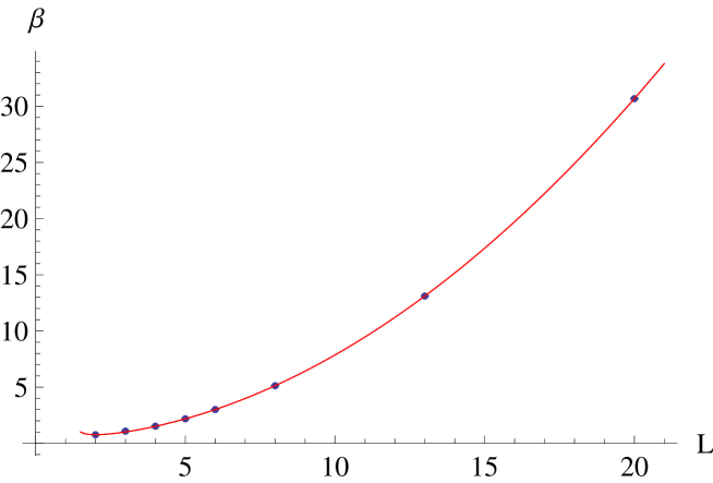
Figure 1: Critical couplings of $3D$ $Z(N)$ vector models plotted versus $N$ (dots) together with the fitting curve given in (18) (solid line). The error bars on the critical couplings are smaller than symbols.

4.3 Critical indices and hyperscaling relation

The procedure to determine the critical index $\nu$ is also inspired by Ref. [22]: for each lattice size $L$ the known function $U_{L}^{(M)}(\beta)$ is used to determine $dU_{L}^{(M)}(\beta)/d\beta$; from this, the derivative of $U_{L}^{(M)}$ with respect to the rescaled coupling $x=(\beta-\beta_{\rm c})L^{1/\nu}$ can be calculated,

$$\frac{dU_{L}^{(M)}}{dx}=\frac{dU_{L}^{(M)}}{d\beta}L^{1/\nu}\;.$$ (19)

The best estimate of $\nu$ is found by minimizing the deviation of $dU_{L}^{(M)}/dx$ with respect to a constant value. The minimization can be done at $\beta_{\rm c}$ or at any other value $\beta_{\rm f}\approx\beta_{\rm c}$ defined as the point where $U_{L}^{(M)}$ on a given lattice becomes equal to some fixed value. The resulting values for $\nu$, summarized in Table 2, do not differ within error bars.

Table 2: Critical index $\nu$ of $3D$ $Z(N)$ vector models determined by the fit procedure described in the text for different choices of the minimum lattice size $L_{\rm min}$; the $\chi^{2}$ given in the last column is the reduced one

$N$	$L_{\min}$	$\nu$	$\chi^{2}_{\nu}$
2	8	0.6253(5)	2.53
	16	0.6280(7)	1.21
	24	0.6306(8)	0.90
4	8	0.62661(11)	1.96
	16	0.62793(12)	1.93
	24	0.62933(12)	1.07
5	8	0.6675(5)	1.49
	16	0.6698(4)	0.94
	24	0.6681(8)	1.13
6	8	0.6687(12)	4.12
	16	0.6739(10)	1.53
	24	0.6756(17)	2.10

$N$	$L_{\min}$	$\nu$	$\chi^{2}_{\nu}$
8	8	0.6678(5)	5.41
	16	0.6720(4)	1.96
	24	0.6748(2)	1.43
13	8	0.6670(7)	3.68
	16	0.6709(9)	2.42
	24	0.6723(17)	2.67
20	8	0.6689(7)	4.08
	16	0.6730(4)	1.04
	24	0.6739(7)	1.36

The critical indices $\beta/\nu$ and $\gamma/\nu$ can be extracted from the FSS analysis of the magnetization $M_{L}$ and its susceptibility $\chi_{L}^{(M)}$, according to the following fitting functions,

$$M_{L} = A_{1}L^{-\beta/\nu}(1+B_{1}L^{-\delta})\ ,$$

$$\chi_{M_{L}} = A_{2}L^{\gamma/\nu}(1+B_{2}L^{-\delta})\ ,$$ (20)

which include also the first subleading corrections. The critical index $\eta$ will then be given by $2-\gamma/\nu$ and the hyperscaling relation $d=2\beta/\nu+\gamma/\nu$ must be satisfied with $d=3$.

In Tables 3 and 4 we summarize the results for the critical indices, when the FSS analysis is performed at $\beta$ fixed at the central value of the determination of $\beta_{\rm c}$. Results are given for the cases when the subleading corrections, depending on the exponent $\delta$, are included in neither fit, in both fits or only in one of them. When considered, the exponent $\delta$ has been fixed to the value $0.53/\nu$, as in the $3D$ $XY$ model. Varying $\delta$ in a wide interval does not give any significant change in the results.

In Tables 5, 6, 7 we summarize the values of the critical indices obtained by two alternative methods: (i) performing the fit with the functions given in (20) not at $\beta_{\rm c}$, but at the pseudocritical $\beta_{\rm pc}$ which maximizes the susceptibility $\chi_{L}^{(M)}$ (column two); (ii) performing the fit at a $\beta_{\rm f}$ defined as the point where $U_{L}^{(M)}$ on a given lattice becomes equal to some fixed value ${U_{L,{\rm f}}^{(M)}}$; as these fixed values, we chose ${U_{L,{\rm crit}}^{(M)}}$ – our estimate for the intersection point of the $U_{L}^{(M)}$ curves at different lattice sizes (column three), then a slightly larger value than this (column four) and slightly smaller value (column five) (for $N>4$, ${U_{L,{\rm f}}^{(M)}}=0.588$ in column three; ${U_{L,{\rm f}}^{(M)}}=0.60$ in column four; ${U_{L,{\rm f}}^{(M)}}=0.57$ in column five); in all cases, the fit was done including data from lattice sizes with $L_{\rm min}=24$.

Table 3: Critical indices $\beta/\nu$ and $\gamma/\nu$ of $3D$ $Z(N)$ vector models with $N=2,4,5,6$, determined by the fits in Eqs. (20), for different choices of the minimum lattice size $L_{\rm min}$. The $\chi^{2}$ of the two fits, given in columns four and six, are the reduced one. Column seven gives the dimension $d$ derived from the hyperscaling relation $d=2\beta/\nu+\gamma/\nu$, while column eight contains the values of $\eta=2-\gamma/\nu$. The three sets of parameters corresponding to the same $L_{\rm min}$ refer to the cases of subleading corrections (term with the exponent $\delta$ in Eqs. (20)) included (i) in neither fit, (ii) only in the fit for $\gamma/\nu$, (iii) in both fits.

$N$	$L_{\min}$	$\beta/\nu$	$\chi^{2}_{\beta/\nu}$	$\gamma/\nu$	$\chi^{2}_{\gamma/\nu}$	$d$	$\eta$
2	8	0.5065(3)	1.32	2.002(2)	26.1	3.015(3)	-0.002(2)
		0.5065(3)	1.32	1.9608(17)	0.73	2.974(2)	0.0392(17)
		0.5074(16)	1.38	1.9608(17)	0.73	2.976(5)	0.0392(17)
	16	0.5066(6)	1.50	1.9908(14)	2.91	3.004(2)	0.0092(14)
		0.5066(6)	1.50	1.962(4)	0.58	2.976(5)	0.038(4)
		0.515(3)	1.08	1.962(4)	0.58	2.993(11)	0.038(4)
	24	0.5058(9)	0.87	1.9851(14)	0.90	2.997(3)	0.0149(14)
		0.5058(9)	0.87	1.971(11)	0.82	2.982(12)	0.029(11)
		0.516(7)	0.75	1.971(11)	0.82	3.00(2)	0.029(11)
4	8	0.5022(6)	7.05	2.007(3)	23.5	3.0012(4)	-0.007(3)
		0.5022(6)	7.05	1.954(2)	0.69	2.958(3)	0.046(2)
		0.5100(19)	3.36	1.954(2)	0.69	2.974(6)	0.046(2)
	16	0.5020(7)	7.46	2.002(2)	12.2	3.006(4)	-0.002(2)
		0.5020(7)	7.46	1.955(2)	0.70	2.959(4)	0.045(2)
		0.514(2)	2.37	1.955(2)	0.70	2.982(7)	0.045(2)
	24	0.5018(9)	7.47	1.998(2)	6.95	3.001(4)	0.002(2)
		0.5018(9)	7.47	1.955(3)	0.76	2.959(5)	0.045(3)
		0.517(2)	1.69	1.955(3)	0.76	2.989(8)	0.045(3)
5	8	0.5106(2)	3.34	1.998(3)	29.8	3.019(3)	0.002(3)
		0.5106(2)	3.34	1.954(2)	0.90	2.975(2)	0.046(2)
		0.5091(12)	3.16	1.954(2)	0.90	2.972(4)	0.046(2)
	16	0.5113(3)	1.85	1.9857(14)	2.27	3.008(2)	0.0143(14)
		0.5113(3)	1.85	1.963(6)	0.94	2.986(7)	0.037(6)
		0.5157(17)	1.11	1.963(6)	0.94	2.995(9)	0.037(6)
	24	0.5101(3)	0.62	1.982(2)	1.81	3.002(2)	0.018(2)
		0.5101(3)	0.62	1.959(16)	1.52	2.980(17)	0.041(16)
		0.512(3)	0.74	1.959(16)	1.52	2.98(2)	0.041(16)
6	8	0.5077(2)	3.36	2.007(4)	47.5	3.022(4)	-0.007(4)
		0.5077(2)	3.36	1.949(2)	0.98	2.964(2)	0.051(2)
		0.5071(12)	3.59	1.949(2)	0.98	2.963(4)	0.051(2)
	16	0.5078(2)	0.88	1.990(2)	4.63	3.006(2)	0.010(2)
		0.5078(2)	0.88	1.947(7)	0.84	2.963(7)	0.053(7)
		0.5121(12)	0.34	1.947(7)	0.84	2.971(9)	0.053(7)
	24	0.5070(3)	0.45	1.983(2)	1.76	2.997(3)	0.017(2)
		0.5070(3)	0.45	1.95(3)	1.85	2.97(3)	0.05(3)
		0.510(4)	0.58	1.95(3)	1.85	2.97(4)	0.05(3)

Table 4: Same as Table 3 for $3D$ $Z(N)$ vector models with $N=8,13,20.$

$N$	$L_{\min}$	$\beta/\nu$	$\chi^{2}_{\beta/\nu}$	$\gamma/\nu$	$\chi^{2}_{\gamma/\nu}$	$d$	$\eta$
8	8	0.5083(2)	4.00	2.006(3)	66.0	3.023(3)	-0.006(4)
		0.5083(2)	4.00	1.952(2)	1.57	2.968(2)	0.048(2)
		0.5082(9)	4.28	1.952(2)	1.57	2.968(4)	0.048(2)
	16	0.5085(3)	2.87	1.992(2)	10.5	3.009(2)	0.008(2)
		0.5085(3)	2.87	1.947(6)	2.04	2.964(6)	0.053(6)
		0.5136(13)	1.33	1.947(6)	2.04	2.974(9)	0.053(6)
	24	0.5079(5)	3.52	1.983(2)	4.57	2.999(3)	0.017(2)
		0.5079(5)	3.52	1.944(16)	2.86	2.959(17)	0.056(16)
		0.519(3)	1.43	1.944(16)	2.86	2.98(2)	0.056(16)
13	8	0.5087(3)	8.22	2.011(3)	52.5	3.028(4)	-0.011(3)
		0.5087(3)	8.22	1.956(2)	1.45	2.973(3)	0.044(2)
		0.5055(13)	6.28	1.956(2)	1.45	2.967(5)	0.044(2)
	16	0.5097(3)	2.05	1.994(2)	6.87	3.014(2)	0.006(2)
		0.5097(3)	2.05	1.949(6)	1.48	2.969(7)	0.051(6)
		0.5137(17)	1.48	1.949(6)	1.48	2.977(10)	0.051(6)
	24	0.5088(5)	2.12	1.985(2)	2.06	3.003(3)	0.015(2)
		0.5088(5)	2.12	1.958(15)	1.61	2.976(16)	0.042(15)
		0.514(4)	2.10	1.958(15)	1.61	2.99(2)	0.042(15)
20	8	0.5076(3)	9.69	2.006(3)	65.7	3.022(4)	-0.006(3)
		0.5076(3)	9.69	1.952(2)	1.94	2.967(2)	0.048(2)
		0.5067(14)	10.0	1.952(2)	1.94	2.965(5)	0.048(2)
	16	0.5080(3)	4.48	1.9905(18)	7.25	3.007(2)	0.0095(18)
		0.5080(3)	4.48	1.953(5)	1.82	2.969(6)	0.047(5)
		0.5148(16)	1.92	1.953(5)	1.82	2.983(9)	0.047(5)
	24	0.5074(7)	5.80	1.985(2)	4.68	2.999(4)	0.015(2)
		0.5074(7)	5.80	1.941(13)	2.33	2.956(15)	0.059(13)
		0.523(2)	0.85	1.941(13)	2.33	2.987(18)	0.059(13)

Table 5: Critical indices of $3D$ $Z(N)$ vector models obtained from two alternative methods (see the text); the results of the first alternative are given in column two, those of the second alternative (three variants) in columns from three to five. The legenda for the entries in each large cell is the following: $\eta=2-\gamma/\nu$ (first line), $\beta/\nu$ with its $\chi^{2}$ (second line), $\gamma/\nu$ with its $\chi^{2}$ (third line) and the dimension $d=2\gamma/\nu+\beta/\nu$ (fourth line). Subleading corrections (term with the exponent $\delta$) were not included in either fits.

$N$	$\beta_{\rm pc}$, $\chi^{(M)}_{L}$ max	$\beta_{\rm f},{U_{L}^{(M)}}_{\rm f}={U_{L}^{(M)}}_{\rm crit}$	$\beta_{\rm f},{U_{L}^{(M)}}_{\rm f}>{U_{L}^{(M)}}_{\rm f}$	$\beta_{\rm f},{U_{L}^{(M)}}_{\rm f}<{U_{L}^{(M)}}_{\rm f}$
2	$\eta$=0.017(2)	0.0172(13)	0.0162(19)	0.0141(15)
	$\beta/\nu$=0.512(3), $\chi^{2}$=6.18	0.504(2) 1.93	0.504(2) 1.93	0.5049(12) 1.80
	$\gamma/\nu$=1.983(2), $\chi^{2}$=1.53	1.9828(13) 0.55	1.9838(19) 1.48	1.9859(15) 2.02
	$d$=3.006(9)	2.990(5)	2.991(5)	2.996(4)
4	0.0106(18)	0.0182(18)	0.018(3)	0.016(2)
	0.4983(17) 43.3	0.493(2) 36.6	0.493(2) 36.6	0.493(2) 36.6
	1.9894(18) 4.28	1.9818(18) 1.09	1.982(2) 2.54	1.984(2) 2.49
	2.986(5)	2.968(7)	2.967(8)	2.970(7)
5	0.0218(13)	0.0210(10)	0.0219(14)	0.0218(13)
	0.5106(9) 3.56	0.5103(4) 1.66	0.5088(7) 3.61	0.5106(9) 3.56
	1.9762(13) 0.76	1.9790(10) 0.76	1.9781(14) 0.75	1.9782(13) 0.76
	2.999(3)	2.9996(18)	2.996(2)	2.999(3)
6	0.0227(16)	0.0179(14)	0.0182(12)	0.021(2)
	0.5052(9) 6.04	0.5052(9) 6.04	0.5052(9) 6.04	0.5101(13) 3.49
	1.9773(16) 1.92	1.9821(14) 1.06	1.9818(12) 1.37	1.979(2) 0.85
	2.988(3)	2.992(3)	2.992(3)	2.999(4)
8	0.0213(15)	0.0176(16)	0.0172(13)	0.0222(19)
	0.511(4) 180.	0.5075(6) 4.12	0.5083(8) 14.1	0.5098(4) 0.73
	1.9787(15) 1.06	1.9824(16) 1.91	1.9828(13) 1.74	1.9778(19) 1.12
	3.000(11)	2.997(2)	2.999(2)	2.998(2)
13	0.0199(12)	0.0168(16)	0.0146(14)	0.0149(12)
	0.5078(9) 3.72	0.5075(8) 4.16	0.5092(11) 20.0	0.5063(8) 10.1
	1.9801(12) 0.90	1.9832(16) 1.24	1.9854(14) 1.73	1.9851(12) 2.07
	2.996(3)	2.998(3)	3.004(3)	2.998(3)
20	0.0221(18)	0.0166(13)	0.005(9)	0.0196(12)
	0.5062(15) 11.8	0.5071(5) 3.43	0.5034(7) 16.1	0.5094(9) 10.7
	1.9779(18) 2.35	1.9834(13) 1.26	1.995(9) 123.	1.9804(12) 2.00
	2.990(4)	2.998(3)	3.002(10)	2.999(3)

Table 6: Same as Table 5, with subleading corrections (term with the exponent $\delta$) included only in the fits for $\gamma/\nu$.

$N$	$\beta_{\rm pc}$, $\chi_{M_{L}}$ max	$\beta_{\rm f},{U_{L}^{(M)}}_{\rm f}={U_{L}^{(M)}}_{\rm crit}$	$\beta_{\rm f},{U_{L}^{(M)}}_{\rm f}>{U_{L}^{(M)}}_{\rm f}$	$\beta_{\rm f},{U_{L}^{(M)}}_{\rm f}<{U_{L}^{(M)}}_{\rm f}$
2	0.03(2)	0.032(11)	0.025(18)	0.033(10)
	0.512(3) 6.18	0.504(2) 1.93	0.504(2) 1.93	0.5049(12) 1.80
	1.97(2) 1.74	1.968(11) 0.49	1.975(8) 1.67	1.967(10) 1.68
	3.00(3)	2.975(15)	2.98(2)	2.977(13)
4	0.041(5)	0.039(12)	0.049(14)	0.044(6)
	0.4983(17) 43.3	0.493(2) 36.6	0.493(2) 36.6	0.493(2) 36.6
	1.959(5) 1.15	1.961(12) 0.89	1.951(14) 1.74	1.956(6) 0.80
	2.956(8)	2.947(17)	2.936(19)	2.942(11)
5	0.036(8)	0.037(5)	0.029(12)	0.036(8)
	0.5106(9) 3.56	0.5103(4) 1.66	0.5088(7) 3.61	0.5106(9) 3.56
	1.964(8) 0.67	1.963(5) 0.44	1.971(12) 0.80	1.964(8) 0.67
	2.985(10)	2.984(5)	2.989(13)	2.985(10)
6	0.040(11)	0.038(10)	0.030(5)	0.026(16)
	0.5052(9) 6.04	0.5052(9) 6.04	0.5052(9) 6.04	0.5101(13) 3.49
	1.960(11) 1.68	1.962(10) 0.77	1.970(5) 0.95	1.974(16) 0.97
	2.970(13)	2.972(11)	2.980(7)	2.994(19)
8	0.038(13)	0.042(10)	0.034(4)	0.048(12)
	0.511(4) 180.	0.5075(6) 4.12	0.5083(8) 14.1	0.5098(4) 0.73
	1.962(13) 1.00	1.958(10) 1.27	1.966(4) 0.65	1.952(12) 0.82
	2.98(2)	2.973(11)	2.983(6)	2.972(13)
13	0.031(10)	0.038(9)	0.029(7)	0.038(6)
	0.5078(9) 3.72	0.5075(8) 4.16	0.5092(11) 20.0	0.5063(8) 10.1
	1.969(10) 0.89	1.962(9) 0.87	1.971(7) 1.37	1.962(6) 1.12
	2.984(12)	2.977(11)	2.990(10)	2.975(8)
20	0.036(10)	0.036(8)	0.01(6)	0.033(4)
	0.5062(15) 11.8	0.5071(5) 3.43	0.5034(7) 16.1	0.5094(9) 10.7
	1.964(10) 2.10	1.964(8) 0.84	1.99(6) 134.	1.967(4) 1.00
	2.976(13)	2.978(9)	3.00(6)	2.985(6)

Table 7: Same as Table 5, with subleading corrections (term with the exponent $\delta$) included in both the fits for $\gamma/\nu$ and for $\beta/\nu$.

$N$	$\beta_{\rm pc}$, $\chi_{M_{L}}$ max	$\beta_{\rm f},{U_{L}^{(M)}}_{\rm f}={U_{L}^{(M)}}_{\rm crit}$	$\beta_{\rm f},{U_{L}^{(M)}}_{\rm f}>{U_{L}^{(M)}}_{\rm f}$	$\beta_{\rm f},{U_{L}^{(M)}}_{\rm f}<{U_{L}^{(M)}}_{\rm f}$
2	0.03(2)	0.032(11)	0.025(18)	0.033(10)
	0.534(11) 1.37	0.536(8) 0.63	0.536(8) 0.63	0.524(5) 0.78
	1.97(2) 1.74	1.968(11) 0.49	1.975(8) 1.67	1.967(10) 1.68
	3.04(4)	3.04(2)	3.05(3)	3.01(2)
4	0.041(5)	0.039(12)	0.049(14)	0.044(6)
	0.527(2) 3.51	0.535(3) 1.71	0.535(3) 1.71	0.535(3) 1.71
	1.959(5) 1.15	1.961(12) 0.89	1.951(14) 1.74	1.956(6) 0.80
	3.012(10)	3.032(19)	3.02(2)	3.027(13)
5	0.036(8)	0.037(5)	0.029(12)	0.036(8)
	0.504(6) 3.48	0.5035(13) 0.52	0.500(4) 3.04	0.504(6) 3.48
	1.964(8) 0.67	1.963(5) 0.44	1.971(12) 0.80	1.964(8) 0.67
	2.97(2)	2.970(7)	2.97(2)	2.97(2)
6	0.040(11)	0.038(10)	0.030(5)	0.026(16)
	0.523(2) 0.97	0.523(2) 0.97	0.523(2) 0.97	0.488(4) 0.98
	1.960(11) 1.68	1.962(10) 0.77	1.970(5) 0.95	1.974(16) 0.97
	3.005(17)	3.007(15)	3.015(11)	2.95(2)
8	0.038(13)	0.042(10)	0.034(4)	0.048(12)
	0.58(4) 149.	0.497(3) 1.72	0.497(2) 3.43	0.509(3) 0.82
	1.962(13) 1.00	1.958(10) 1.27	1.966(4) 0.65	1.952(12) 0.82
	3.11(10)	2.952(16)	2.960(8)	2.97(2)
13	0.031(10)	0.038(9)	0.029(7)	0.038(6)
	0.508(6) 4.25	0.494(2) 0.95	0.4924(17) 1.56	0.493(4) 5.99
	1.969(10) 0.89	1.962(9) 0.87	1.971(7) 1.37	1.962(6) 1.12
	2.98(2)	2.951(14)	2.956(11)	2.948(15)
20	0.036(10)	0.036(8)	0.01(6)	0.033(4)
	0.503(9) 13.6	0.497(2) 1.15	0.491(2) 4.35	0.4976(19) 1.99
	1.964(10) 2.10	1.964(8) 0.84	1.99(6) 134.	1.967(4) 1.00
	2.97(2)	2.957(13)	2.98(7)	2.962(8)

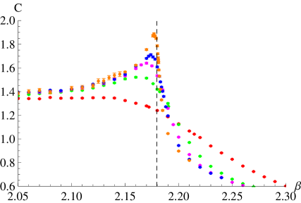
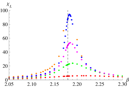
Figure 2: Heat capacity (left) and susceptibility $\chi_{L}^{(M)}$ (right) versus $\beta$ for the $3D$ $Z(5)$ vector model on lattices with $L$ = 8 (red), 16 (green), 24 (violet), 32 (blue) and 64 (orange). The vertical dashed line shows the location of the critical point. The error bars are smaller than symbols.

4.4 Heat capacity and the index $\alpha$

The critical index $\alpha$, determined from the $\nu$ values obtained in the previous subsection by means of the relation $\alpha=2-d\nu$, gets negative values for all $N\geq 5$, meaning that the transition is of order higher than two. In fact, these negative values are very close to that of the $3D$ $XY$ model [22]. However, the plots of the heat capacity (see Fig. 2(left)) clearly show that it diverges in the vicinity of the critical point. Moreover, the maxima of the heat capacity and of the susceptibility $\chi_{L}^{(M)}$ approach the critical point from different sides (see Figs. 2).

This suggests that a different value for the index $\nu$ can be found if a FSS analysis is done on the peak values of the heat capacity, using as fitting function

$$C(L)=AL^{\alpha/\nu}(1+BL^{-\delta})\ ,$$ (21)

where the possible inclusion of subleading corrections has been taken into account. After $\alpha/\nu$ is extracted, from the relation $\alpha=2-d\nu$ the value of $\nu$ can be obtained.

In Table 8 we summarize the results for $\nu$ determined in the described way, with and without the inclusion of the subleading correction term. When considered, the exponent $\delta$ has been fixed to the value $0.5/\nu$. The error estimates given in the table do not include systematic uncertainties brought by the localization of the maximum of the heat capacity by using analytic continuation, which can be unreliable in regions where the heat capacity changes fast. The constant $B$ in front of the subleading correction appears to be of order unity, $B\sim 0.4-0.7$, and does not seem to depend on $N$.

We see that while for $N=2,4$ the resulting $\nu$ agrees with the value of $\nu$ in the $3D$ Ising model, and the agreement improves if we include the subleading correction, for $N>4$ this is not the case. For $N>4$ the difference between the $\nu$ values obtained with and without inclusion of subleading corrections is much smaller than for $N=2,4$. The most important fact is, however, that in all cases the $\nu$ indices obtained in this way are close to $\nu\approx 0.63$ – the critical index for the Ising model. The difference between $\nu$ indices obtained from the $U_{L}^{(M)}$ cumulants and from the heat capacity leads us to conclude that we have two kinds of singularity depending on whether one approaches the critical coupling from above ($3D$ $XY$ model-like singularity) or from below ($3D$ Ising universality class), for $N>4$.

Table 8: Critical index $\nu$ of $3D$ $Z(N)$ vector models with $N=2,4,5,6,8,13,20$ determined by the fit given in Eq. (21) on the peak of the heat capacity, for different choices of the minimum lattice size $L_{\rm min}$. The two sets of parameters refer to the cases of subleading corrections (term with the exponent $\delta$ in Eqs. (21)) not included in the fit or included with $\delta$ fixed at $0.5/\nu$ The $\chi^{2}$ of the fits, given in columns four and six, are the reduced ones.

		no subl. corr.		with subl. corr.
$N$	$L_{\min}$	$\nu$	$\chi^{2}_{\nu}$	$\nu$	$\chi^{2}_{\nu}$
2	8	0.6108(4)	8.00	0.6185(4)	0.44
	16	0.6132(4)	1.37	0.6214(16)	0.42
	24	0.6143(6)	1.04	0.623(4)	0.46
	32	0.6154(7)	0.51	0.627(7)	0.42
4	8	0.6117(9)	3.27	0.6223(17)	0.79
	16	0.6146(9)	1.16	0.629(4)	0.72
	24	0.6168(14)	0.81	0.634(9)	0.57
5	8	0.6047(6)	5.35	0.639(2)	0.89
	16	0.6338(12)	1.94	0.6410(8)	0.08
	24	0.6360(6)	0.22	0.6409(15)	0.17
6	8	0.6300(10)	21.3	0.640(5)	16.5
	16	0.6348(8)	1.78	0.642(3)	0.97
	24	0.6360(10)	1.57	0.646(3)	0.61
8	8	0.6293(6)	78.6	0.6385(18)	19.3
	16	0.6320(4)	11.4	0.637(3)	9.71
	24	0.6336(3)	2.40	0.631(10)	11.8
13	8	0.6294(6)	68.6	0.6411(3)	2.11
	16	0.6323(4)	9.04	0.6425(7)	1.80
	24	0.6340(4)	2.52	0.6442(13)	1.87
20	8	0.6285(5)	53.8	0.6428(8)	6.79
	16	0.6304(3)	5.19	0.6472(17)	5.19
	24	0.6314(3)	2.35	0.657(3)	2.84

5 Symmetric phase

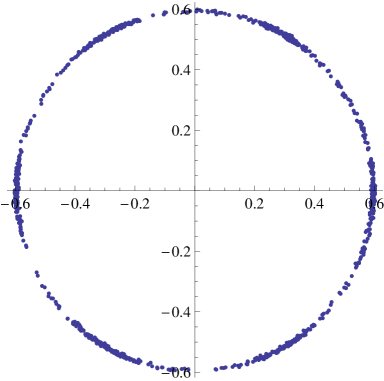
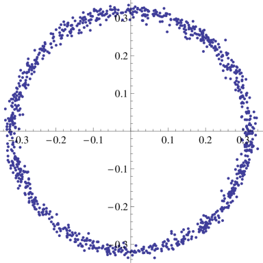
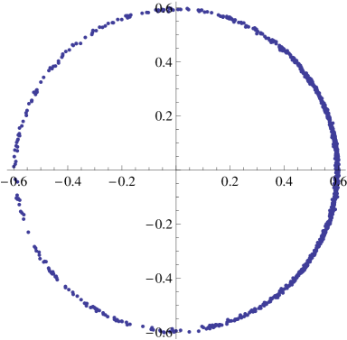
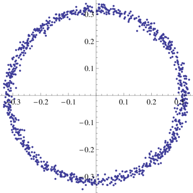
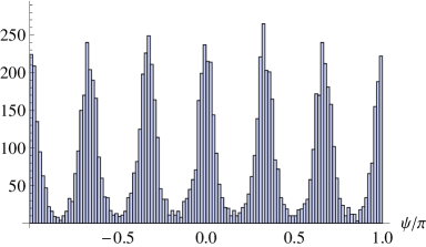
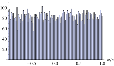
Figure 3: Scatter plots for the magnetization (top) and the rotated magnetization (middle), histogram of the magnetization angle (bottom) for the $3D$ $Z(6)$ vector model on a $64^{3}$ lattice for $\beta=2.7$ (left) and $\beta=2.97$ (right).

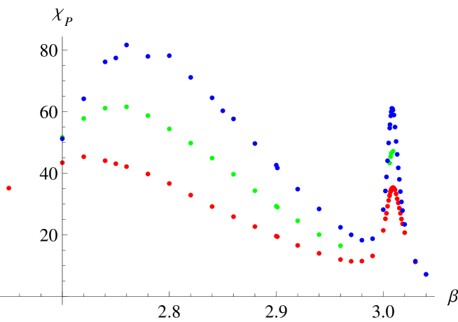
Figure 4: Population susceptibility $\chi_{P}$ for the $3D$ $Z(6)$ vector model on lattices with $L$ = 48 (red), 56 (green) and 64 (blue) versus $\beta$. The error bars are not shown.

Another interesting phenomenon we have encountered during our study is the appearance of a symmetric phase just below $\beta_{\rm c}$ for all $N\geq 5$. That such phase exists in the vector $Z(6)$ spin model has been known for a long time [12, 13, 14]. Here we confirm its existence for all vector $Z(N\geq 5)$ LGTs. The phase exhibits itself, e.g., in the behavior of magnetization. As an example, we give in Fig 3 the scatter plots of magnetization and rotated magnetization, together with the histogram of the magnetization angle for $Z(6)$ on a $64^{3}$ lattice. One sees that below the critical coupling at $\beta=2.97$ the symmetry is not broken on this lattice. Only starting from approximately $\beta=2.7$ one can observe the appearance of a symmetry-broken phase. In addition, we have studied the behavior of the population susceptibility below $\beta_{\rm c}=3.00683$. Fig 4 shows that it has a second broad maximum, which slowly moves to $\beta_{\rm c}=3.00683$ with increasing lattice size. A similar picture is observed for all $N\geq 5$. While, however, for $N=5$ the peak of the population susceptibility moves rather fast and practically collapses with the peak at the critical coupling on the largest available lattice $L=96$, for larger $N$ the peak stays rather far from the corresponding critical coupling, even for $L=96$ (with our data we cannot even exclude a situation when the convergence of the second maximum is logarithmic). We can imagine two scenarios to explain such behavior:

1. This symmetric phase exists only in finite volume. When the lattice size increases, the second maximum approaches the critical coupling and, eventually, the symmetric region shrinks and disappears. The explanation proposed in [13, 14] might work in this case, too. Namely, the symmetric phase on the finite lattice is a phase with a very small mass gap and describes a crossover region to the symmetry-broken phase.

2. For $N>5$ the second maximum of the population susceptibility stays away from the critical couplings even in the infinite volume limit. In this case it might correspond to some higher order phase transition and the symmetric phase with tiny or even vanishing mass gap exists also in the thermodynamic limit.

In both cases it is tempting to speculate that this symmetric region is reminiscent of the massless phase which appears in these models at finite temperature [17]. Whichever scenario of the above two is realized, one needs to study the models on much larger lattices to uncover it.

6 Summary

In this paper we have studied the $3D$ $Z(N)$ LGT at zero temperature aiming at shedding light on the nature of phase transitions in these models for $N\geq 4$. This study was based on the exact duality transformations of the gauge models to generalized $3D$ $Z(N)$ spin models. In Section 2 we presented an overview of the exact relation between couplings of these two models. In Section 3 we have studied the models analytically using a version of the phenomenological RG based on the preservation of the mass gap combined with a cluster decimation approximation. This study provided us with an approximate location of the critical couplings as well as with the value of the index $\nu$. These calculations show that the index $\nu$ is approximately the same for $N=2,4$, $\nu\approx 0.616$, indicating that these two models might belong to the same universality class. We find $\nu>2/3$ and approximately equal for $N>4$. Hence, $Z(N>4)$ vector LGTs belong to a different universality class.

The numerical part of the work has been devoted to the localization of the critical couplings, computation of the various critical indices and check of the hyperscaling relation. The main results can be shortly summarized as follows:

• We have determined numerically the position of the critical couplings for various $Z(N)$ models. For $N=2,3$ we find a reasonable agreement with the values quoted in the literature. For larger $N$, we have significantly improved the values given in [10]. This allowed us to improve the scaling formula for the critical couplings with $N$.

• The critical indices $\nu$ and $\eta$ derived here for $N=2,4$ suggest that these models are in the universality class of the $3D$ Ising model, while our results for all $N>4$ hint all vector $Z(N\geq 5)$ LGTs belong to the universality class of the $3D$ $XY$ model. This is especially evident from the value of the index $\nu$, which stays very close to the $XY$ value, $\nu\approx 0.6716$, given in [22]. The index $\alpha$ in this case takes a small negative value. It thus follows that a third order phase transition takes place for $N\geq 5$.

• A careful investigation of the specific heat and of the index $\alpha$ extracted from it suggests however a more complicated picture of the critical behavior. In this case we find a value which roughly agrees with the value of $3D$ Ising model for all $N$ studied. The fact that we observe two different values of the index $\alpha$ dependently on whether we approach the critical point from below or from above leads to the conclusion that the first derivative of the free energy could exhibit a cusp in the thermodynamic limit if $N>4$.

• Our data also revealed the existence of a symmetric phase for all $Z(N)$ vector LGTs if $N>4$. However, substantially larger lattices are required to see if this phase survives the transition to the thermodynamic limit.

7 Acknowledgments

The work of Ukrainian co-authors was supported by the Ukrainian State Fund for Fundamental Researches under the grant F58/384-2013. Numerical simulations have been partly carried out on Ukrainian National GRID facilities. O.B. thanks for warm hospitality the Dipartimento di Fisica dell’Università della Calabria and the INFN Gruppo Collegato di Cosenza during the final stages of this investigation.

References

- [1] D. Horn, M. Weinstein and S. Yankielowicz, Phys. Rev. D 19 (1979) 3715.
- [2] A. Ukawa, P. Windey, A.H. Guth, Phys. Rev. D 21 (1980) 1013.
- [3] M.B. Einhorn, R. Savit, and E. Rabinovici, Nucl. Phys. B 170 (1980) 16.
- [4] M. Caselle, M. Hasenbusch, M. Panero, JHEP 0301 (2003) 057; M. Caselle, M. Hasenbusch, Nucl. Phys. B 470 (1996) 435.
- [5] R.V. Gavai, F. Karsch, B. Petersson, Nucl. Phys. B 322 (1989) 738.
- [6] M. Fukugita, H. Mino, M. Okawa, A. Ukawa, J. Stat. Phys. 59 (1990) 1397.
- [7] A. Bazavov, B.A. Berg, Phys. Rev. D 75 (2007) 094506.
- [8] A. Bazavov, B.A. Berg, S. Dubey, Nucl. Phys. B 802 (2008) 421.
- [9] M. Hellmund, W. Janke, Phys. Rev. E 74 (2006) 051113.
- [10] G. Bhanot and M. Creutz, Phys. Rev. D 21 (1980) 2892.
- [11] A. Polyakov, Nucl. Phys. B 120 (1977) 429; T. Banks, J. Kogut, R. Myerson, Nucl. Phys. B 129 (1977) 493; M. Göpfert, G. Mack, Commun. Math. Phys. 81 (1981) 97.
- [12] P.D. Scholten, L.J. Irakliotis, Phys. Rev. B 48 (1993) 1291.
- [13] S. Miyashita, J. Phys. Soc. Japan, 66 (1997) 3411.
- [14] M. Oshikawa, Phys. Rev. B 61 (2000) 3430.
- [15] O. Borisenko, V. Chelnokov, G. Cortese, R. Fiore, M. Gravina, A. Papa, I. Surzhikov, Phys. Rev. E 86 (2012) 051131.
- [16] O. Borisenko, V. Chelnokov, G. Cortese, R. Fiore, M. Gravina, A. Papa, I. Surzhikov, PoS LATTICE 2012 270 [arXiv:1212.1051 [hep-lat]].
- [17] O. Borisenko, V. Chelnokov, G. Cortese, M. Gravina, A. Papa, I. Surzhikov, Nucl. Phys. B 870 (2013) 159.
- [18] M.P. Nightingale, Physica 83A (1976) 561; J. Appl. Phys. 53 (1982) 7927.
- [19] M.A. Yurishchev, J. Phys.: Condens. Matter 5 (1993) 8075.
- [20] O. Borisenko, V. Chelnokov, V. Kushnir, in preparation.
- [21] R.E. Goldstein, J.S. Walker, J.Phys. A: Math.Gen. 18 (1985) 1275.
- [22] M. Campostrini, M. Hasenbusch, A. Pelissetto, P. Rossi, E. Vicari, Phys. Rev. B 63 (2001) 214503.