The TDHF Code Sky3D

Abstract

The nuclear mean-field model based on Skyrme forces or related density functionals has found wide-spread application to the description of nuclear ground states, collective vibrational excitations, and heavy-ion collisions. The code Sky3D solves the static or dynamic equations in a three-dimensional Cartesian mesh with isolated or periodic boundary conditions and no further symmetry assumptions. Pairing can be included in the BCS approximation. The code is implemented with a view to allow easy modifications for including additional physics or special analysis of the results.

PROGRAM SUMMARY

Title: The TDHF Code Sky3D
Authors: J. A. Maruhn, P.-G. Reinhard, P. D. Stevenson, and A. S. Umar.
Program Title: Sky3D
Journal Reference:
Catalogue identifier:
Licensing provisions: none
Programming language: Fortran 90
Computer: All computers with a Fortran compiler supporting at least Fortran 90.
Operating system: All operating systems with such a compiler. Some of the Makefiles and scripts depend on a Unix-like system and need modification under Windows.
RAM: 1 GB
Number of processors used: no built-in limit, runs under both OpenMP and MPI
Keywords: Nuclear theory, Mean-field models, Nuclear reactions
Classification: 17.16 Theoretical Methods - General, 17.22 Hartree-Fock Calculations, 17.23 Fission and Fusion Processes
External routines/libraries: LAPACK, FFTW3

Nature of problem: The time-dependent Hartree-Fock equations can be used to simulate nuclear vibrations and collisions between nuclei for low energies. This code implements the equations based on a Skyrme energy functional and also allows the determination of the ground-state structure of nuclei through the static version of the equations. For the case of vibrations the principal aim is to calculate the excitation spectra by Fourier-analyzing the time dependence of suitable observables. In collisions, the formation of a neck between nuclei, the dissipation of energy from collective motion, processes like charge transfer and the approach to fusion are of principal interest.

Solution method: The nucleonic wave function spinors are represented on a three-dimensional Cartesian mesh with no further symmetry restrictions. The boundary conditions are always periodic for the wave functions, while the Coulomb potential can also be calculated for an isolated charge distribution. All spatial derivatives are evaluated using the finite Fourier transform method. The code solves the static Hartree-Fock equations with a damped gradient iteration method and the time-dependent Hartree-Fock equations with an expansion of the time-development operator. Any number of initial nuclei can be placed into the mesh in with arbitrary positions and initial velocities.

Restrictions: The reliability of the mean-field approximation is limited by the absence of hard nucleon-nucleon collisions. This limits the scope of applications to collision energies about a few MeV per nucleon above the Coulomb barrier and to relatively short interaction times. Similarly, some of the missing time-odd terms in the implementation of the Skyrme interaction may restrict the applications to even-even nuclei.


Unusual features:
The possibility of periodic boundary conditions and the highly flexible initialization make the code also suitable for astrophysical nuclear-matter applications.

Running time: The running time depends strongly on the size of the grid, the number of nucleons, and the duration of the collision. For a single-processor PC-type computer it can vary between a few minutes and weeks.

1 Introduction

The vast majority of microscopic models of many-body systems rely on a description in terms of the single-particle (s.p.) wave functions. Among them, self-consistent mean-field models (SCMF) automatically generate the optimal one-body potentials corresponding to the s.p. wave functions. A rigorous SCMF is the Hartree-Fock theory (HF) where the s.p. wave functions are determined variationally for a given two-body interaction [1, 2]. A more practical approach is provided by the Density Functional Theory (DFT), which incorporates the involved many-body effects into effective interactions, or effective energy-density functionals. This is a very efficient and successful scheme, widely used in electronic systems [3]. Straightforward HF is unsuitable for nuclei because the free-space two-nucleon force contains a strong short-range repulsion requiring renormalization in the nuclear medium. For this reason, nuclear SCMFs necessarily employ effective interactions or functionals although they often carry the label HF as, e.g, in the Skyrme Hartree-Fock (SHF) method. There are relativistic as well as non-relativistic approaches. For an extensive review see [4].

The description of dynamical processes is even more demanding than the modeling of structure. SCMFs are the also the first method of choice in this domain. The natural extension of HF is time-dependent HF (TDHF) which was proposed as early as 1930 in [5]. Earlier applications were restricted to the linearized regime covering small amplitude motion, see, e. g., [6]. Large scale TDHF calculations became possible in the last few decades with the increasing computing capacities. Again, as in the static case, true TDHF calculations make sense only for electronic systems and even there they are very rare. The overwhelming majority of dynamical SCMF calculations employ, in fact, time-dependent DFT (TDDFT). In electronic systems, this amounts to the time-dependent local density approximation (TDLDA) [3], which is widely used in atoms, molecules, and solids; for examples in nanoparticles see, e. g., [7]. Dynamical SCMFs in nuclei also stay at the level of TDLDA even if they are often named TDHF which happens particularly for dynamical calculations using the Skyrme energy functional. Nuclear TDHF started about forty years ago [8] and has developed since then into a powerful and versatile tool for simulating a great variety of dynamical scenarios. Earlier applications were based mainly on non-relativistic TDHF using the effective Skyrme energy functional [9, 10]. Due to higher numerical demands, relativistic calculations appeared somewhat later [11], but have developed meanwhile equally well to a widely used tool [12, 13].

In this paper, we present a code for TDHF calculations on the basis of the non-relativistic Skyrme energy functional. The code uses a fully three dimensional (3D) representation of wave functions and fields on a Cartesian grid in coordinate space. There are no symmetry restrictions and the full Skyrme energy functional is used including the spin-orbit and most important time-odd terms. Such fully-fledged 3D calculations became possible only over the last decade with the steadily increasing computing capabilities. In fact, early TDHF studies all used restricted representations, axial symmetry and/or reflection symmetries. This limited the possible applications. TDHF experienced a revival during the last ten years when unrestricted 3D calculations became possible. There are several groups performing large scale TDHF studies for various scenarios of nuclear dynamics, see, e.g., [14, 15, 16, 17, 18, 19, 20]. For a recent review see [21]. Such calculations have clearly outgrown the developmental stage. It is an appropriate time to give a broader public access to a 3D TDHF code. This is the goal of this paper. Skyrme HF covers such a broad range of physical phenomena and is relatively involved that efficient computational treatment of 3D simulations requires elaborate numerical methods. We shall make an effort to explain the many necessary ingredients in a comprehensive, and yet compact, manner.

Most recent Skyrme density functionals contain terms such as fractional powers of the density that cannot be related to a two- or three-body interaction. In that sense, the present code solves the TDDFT rather than TDHF equations. Nevertheless, we prefer to keep the name TDHF since it is associated historically with this large field of nuclear reaction theory.

2 General purpose and structure

2.1 Intended applications

The code Sky3D solves the static Hartree-Fock as well as the time-dependent Hartree-Fock (TDHF) equations for interactions of Skyrme-force type in a general three-dimensional geometry. No symmetries of any kind are assumed, so that the code can be used for a wide variety of applications in nuclear structure, collective excitations, and nuclear reactions; of course within the limitations of mean-field theory.

2.2 Specific model implemented

The code in the presented version contains a useful selection of terms in the Skyrme force but by no means all terms that have been included in some recent works. It should still be useful, because (1) for many interesting applications the interest is semi-quantitative so that a Skyrme force fitted with the latest models is not necessary — usually a selection of forces is desired to look at the variability of results, but not a high-accuracy fit of data; (2) the code is written in such a way that additional terms can be added easily. The coding corresponds one-by-one to the analytic formulas in most places except where efficiency demands reordering the calculations.

2.2.1 The single-particle basis

In a mean field theory one seeks to describe the many-body system exclusively in terms of a set of single-particle wave functions $\psi_{\alpha}$ with fractional occupation amplitudes $v_{\alpha}$, i.e.

$$\left\{\psi_{\alpha},v_{\alpha},\alpha=1,...,\Omega\right\}$$ (1a)

where $$\Omega [0,1] u_{\alpha}=\sqrt{1-v_{\alpha}^{2}}$$ denotes the size of the active s.p. space. The occupation amplitude can take values continuously in the interval . The complementary non-occupation amplitude is . A formal definition of the BCS mean-field state reads

$$|\Phi\rangle=\prod_{\alpha>0}\big{(}u_{\alpha}^{\mbox{}}+v_{\alpha}^{\mbox{}}\hat{a}^{+}_{\alpha}\hat{a}^{+}_{\bar{\alpha}}\big{)}|0\rangle$$ (1b)

where $|0\rangle$ is the vacuum state, $\hat{a}^{+}_{\alpha}$ the generator of a Fermion in state $\psi_{\alpha}$, and $\bar{\alpha}$ the time reverse partner to state $\alpha$. We will use variation of the BCS amplitudes $v_{\alpha}^{\mbox{}}$ only in the static part of even-even nuclei where the time reverse partner is unambiguously defined. These amplitudes are kept frozen during dynamical propagation whenever BCS pairing is used for a nucleus.

2.2.2 Local densities and currents

The Skyrme-energy-density functional is defined in terms of only a few local densities and currents. These are the time-even fields

$$\rho_{q} =\displaystyle\sum_{\alpha\in q}\sum_{s}v_{\alpha}^{2}|\psi_{\alpha}(\vec{r},s)|^{2}$$ density

$$\vec{J}_{q} =\displaystyle-{\mathrm{i}}\sum_{\alpha\in q}\sum_{ss^{\prime}}v_{\alpha}^{2}\psi_{\alpha}^{*}(\vec{r},s)\nabla\!\times\!\vec{\sigma}_{ss^{\prime}}\psi^{\mbox{}}_{\alpha}(\vec{r},s^{\prime})$$ spin-orbit dens.

$$\tau_{q} =\displaystyle\sum_{\alpha\in q}\sum_{s}v_{\alpha}^{2}|\nabla\!\psi_{\alpha}(\vec{r},s)|^{2}$$ kinetic density, (2)

the time-odd fields

$$\vec{s}_{q} =\displaystyle\sum_{\alpha\in q}\sum_{ss^{\prime}}v_{\alpha}^{2}\psi^{*}_{\alpha}(\vec{r},s)\vec{\sigma}_{ss^{\prime}}\psi^{\mbox{}}_{\alpha}(\vec{r},s^{\prime})$$ spin density

$$\vec{\jmath}_{q} =\displaystyle\Im{m}\left\{\sum_{\alpha\in q}\sum_{s}v_{\alpha}^{2}\psi^{*}_{\alpha}(\vec{r},s)\nabla\!\psi^{\text{}}_{\alpha}(\vec{r},s)\right\}$$ current density, (3)

and a field with undefined time parity:

$$\xi_{q} =\displaystyle{\sum_{\alpha\in q}\sum_{s}u_{\alpha}v_{\alpha}\psi_{\overline{\alpha}}(\vec{r},s)\psi_{\alpha}}(\vec{r},s)$$ pairing density (4)

where $q$ labels the nucleon species with $q=p$ for protons and $q=n$ for neutrons. A local density/current without $q$ index stands for the total quantity, e.g. $\rho=\rho_{p}+\rho_{n}$ is the total density, and similarly for the other densities/currents.

2.2.3 The energy-density functional

The mean-field equations solved in the code are based on the widely used Skyrme energy functional. For recent reviews see [4, 22]. The functional at the level at which it is used here can be written as

$$E_{\mathrm{tot}}=T+(E_{0}+E_{1}+E_{2}+E_{3}+E_{\mathrm{ls}})+E_{\rm Coulomb}+E_{\rm pair}+E_{\rm corr},$$ (5a)

where the parentheses were used to group the terms arising from the Skyrme force. The various terms read in detail

• $T$: the total kinetic energy calculated as

  $$T=\sum_{q}\frac{\hbar^{2}}{2m_{q}}\int{\mathrm{d}}^{3}r\,\tau_{q}(\vec{r})$$ (5b)

  with $\tau_{q}$ the isospin-specific kinetic density of Eq. (2).

• $E_{0}$: The $b_{0}$ and $b^{\prime}_{0}$-dependent part is

  $$E_{0}=\int{\mathrm{d}}^{3}\!r\,\left(\frac{b_{0}}{2}\rho^{2}-\frac{b_{0}^{\prime}}{2}\sum_{q}\rho_{q}^{2}\right).$$ (5c)

• $E_{1}$: kinetic terms containing the coefficients $b_{1}$ and $b_{1}^{\prime}$:

  $$E_{1}=\int{\mathrm{d}}^{3}\!r\,\left(b_{1}[\rho\tau-{\vec{\jmath}\,}{}^{2}]-b_{1}^{\prime}\sum_{q}[\rho_{q}\tau_{q}-{\vec{\jmath}_{q}}{}^{2}]\right).$$ (5d)

• $E_{2}$: terms containing the coefficients $b_{2}$ and $b_{2}^{\prime}$. They involve the Laplacians of the densities.

  $$E_{2}=\int{\mathrm{d}}^{3}\!r\,\left(-\frac{b_{2}}{2}\rho\Delta\rho+\frac{b_{2}^{\prime}}{2}\sum_{q}\rho_{q}\Delta\rho_{q}\right).$$ (5e)

• $E_{3}$: The many-body contribution is given by

  $$E_{3}=\int{\mathrm{d}}^{3}\!r\,\left(\frac{b_{3}}{3}\rho^{\alpha+2}-\frac{b_{3}^{\prime}}{3}\rho^{\alpha}\sum_{q}\rho_{q}^{2}\right).$$ (5f)

• $E_{\mathrm{ls}}$: the spin-orbit energy

  $$\begin{split}E_{\mathrm{ls}}&=\int{\mathrm{d}}^{3}\!r\,\biggl{(}-b_{4}[\rho\nabla\cdot\vec{J}+\vec{s}\cdot(\nabla\times\vec{\jmath})]\\ &-b_{4}^{\prime}\sum_{q}[\rho_{q}\nabla\cdot\vec{J}_{q}+\vec{s}_{q}\cdot(\nabla\times\vec{\jmath}_{q})]\biggr{)}\end{split}$$ (5g)

• $E_{\mathrm{C}}$: the Coulomb energy. It consists of the standard expression for a charge distribution in its own field (Hartree term) plus the exchange term in the Slater approximation  [23]. The formula is

  $$E_{\mathrm{C}}=\frac{e^{2}}{2}\int{\mathrm{d}}^{3}\!r{\mathrm{d}}^{3}\!r^{\prime}\frac{\rho_{p}(\vec{r})\rho_{p}(\vec{r^{\prime}})}{|\vec{r}-\vec{r^{\prime}}|}-\int{\mathrm{d}}^{3}\!r\,\frac{3e^{2}}{4}\left(\frac{3}{\pi}\right)^{\tfrac{1}{3}}\rho_{p}^{4/3}$$ (5h)

  where $e$ is the elementary charge with $e^{2}=1.43989$ MeV fm.

• $E_{\mathrm{pair}}$: the pairing energy. It consists of a contact pairing interaction involving the pairing densities $\xi_{q}$ augmented by an optional density dependence. The formula is

  $$E_{\rm pair}=\frac{1}{4}\sum_{q\in\{p,n\}}V_{\mathrm{pair,q}}\int{\mathrm{d}}^{3}r\xi^{2}_{q}\left[1-\frac{\rho}{\rho_{0,\mathrm{pair}}}\right]\;.$$ (5i)

  It contains a continuous switch, the parameter $\rho_{0,\mathrm{pair}}$. A pure $\delta$-interaction (DI), also called volume pairing, is recovered for $\rho_{0,\mathrm{pair}}\longrightarrow\infty$. The general case is the density dependent $\delta$-interaction (DDDI). A typical value near matter equilibrium density $\rho_{0,\mathrm{pair}}=0.16$ fm^-3 concentrates pairing to the surface. The most flexible choice is to consider $\rho_{0,\mathrm{pair}}$ as an additional free parameter. Actual adjustments with this option deliver a form of the pairing functional which stays in between the extremes of volume and surface pairing [24].

The term $E_{\rm corr}$ stands for all additional corrections from correlations beyond the mean field that might be added. Most calculations include at least the center-of-mass correction $E_{\mathrm{cm}}$. For deformed nuclei this should be augmented by a rotational correction and for soft nuclei by correlations from all low-energy quadrupole motions [25]. So far, these correlations are usually added a posteriori after static calculations. A fully variational treatment and a dynamical propagation of the c.m. correction is extremely involved and usually not considered. We aim predominantly at dynamical simulations and thus here ignore all such correlations, using

$$E_{\mathrm{cm}}=0\quad.$$ (6)

This has to be taken into account when comparing ground state energies from this code with results from other static codes which contain a c.m. correction $E_{\mathrm{cm}}\neq 0$. However, one has to take into account that there are two different ways to perform the c.m. correction. They are selected by the parameter zpe. One strategy is to augment the energy by $E_{\mathrm{cm}}$ a posteriori. We associate this option with zpe=1. This means that in our code nothing is done. The other strategy is to modify the nucleon mass by $m\longrightarrow m-m/A$ and to not have a posteriori correction. This way is chosen in a couple of traditional parametrizations, e.g., in SkM^∗ [26]. We keep this option for consistency and associate it with zpe=1. But note that this choice runs into inconsistencies in collisions and fragmentation as it employs only the total mass number $A$ and cannot account for the masses of the fragments.

The functional in the above form contains the minimal number of terms which are needed to guarantee Galilean invariance [27, 22] and so to allow performance of TDHF calculations which respect all basic conservation laws. We ignore the tensor spin-orbit terms and spin-spin couplings [4, 28, 22]. These may be important for magnetic excitations [22] and odd nuclei [29] which are, however, not the prime focus of TDHF studies.

2.2.4 Force coefficients

The above formulation in terms of the Skyrme energy functional introduces the force parameters $b_{0}$, $b^{\prime}_{0}$, … $b^{\prime}_{4}$ naturally as the factors in front of each contribution in the terms (5c). Traditionally, the functional is deduced from a Skyrme force which is a density-dependent, zero-range interaction [30]. The $t$ and $x$ coefficients in this Skyrme-force definition are related to the $b$ coefficients in the functional definition as

$$\begin{split}b_{0}&=t_{0}\,\left(1+\tfrac{1}{2}x_{0}\right)\\ b_{0}^{\prime}&=t_{0}\,\left(\tfrac{1}{2}+x_{0}\right)\\ b_{1}&=\tfrac{1}{4}\left[t_{1}\,\left(1+\tfrac{1}{2}x_{1}\right)+t_{2}\,\left(1+\tfrac{1}{2}x_{2}\right)\right]\\ b_{1}^{\prime}&=\tfrac{1}{4}\left[t_{1}\,\left(\tfrac{1}{2}+x_{1}\right)-t_{2}\,\left(\tfrac{1}{2}+x_{2}\right)\right]\\ b_{2}&=\tfrac{1}{8}\left[3t_{1}\,\left(1+\tfrac{1}{2}x_{1}\right)-t_{2}\,\left(1+\tfrac{1}{2}x_{2}\right)\right]\\ b_{2}^{\prime}&=\tfrac{1}{8}\left[3t_{1}\,\left(\tfrac{1}{2}+x_{1}\right)+t_{2}\,\left(\tfrac{1}{2}+x_{2}\right)\right]\\ b_{3}&=\tfrac{1}{4}t_{3}\left(1+\tfrac{1}{2}x_{3}\right)\\ b_{3}^{\prime}&=\tfrac{1}{4}t_{3}\left(\tfrac{1}{2}+x_{3}\right)\\ b_{4}&=\tfrac{1}{2}t_{4}\end{split}$$ (7)

The coefficient $b_{4}^{\prime}$ is usually fixed as $b^{\prime}_{4}=\frac{1}{2}t_{4}$ for most traditional Skyrme forces. More recent variants of Skyrme forces (SkI3 etc.) handle it as a separate free parameter [31]. In addition to the $b$ and $b^{\prime}$ parameters, there is the power coefficient in the (originally) three-body term, which is usually called $\alpha$, but in the code is referred to as power. The input of the force to the code is done in terms of the $t_{i}$, $x_{i}$ parameters.

2.2.5 The single-particle Hamiltonian

The mean-field Hamiltonian $\hat{h}$ is derived from the energy functional of Section 2.2.3 by variation $\partial_{\psi_{\alpha}^{*}}E=\hat{h}\psi_{\alpha}$. It reads in detail

$$\begin{split}\hat{h}_{q}&=U_{q}(\vec{r})-\nabla\cdot\left[B_{q}(\vec{r})\nabla\right]+{\mathrm{i}}\vec{W}_{q}\cdot(\vec{\sigma}\times\nabla)+\vec{S}_{q}\cdot\vec{\sigma}\\ &-\frac{{\mathrm{i}}}{2}\left[(\nabla\cdot\vec{A}_{q})+2\vec{A}_{q}\cdot\nabla\right]\,,\end{split}$$

with $$q\in\{p,n\}$$ as usual distinguishing the different Hamiltonians for protons and neutrons. For the protons the Coulomb potential is also added. The first term is the local part of the mean field, which acts on the wave functions like a local potential. It is defined as

$$\begin{split}U_{q}&=b_{0}\rho-b_{0}^{\prime}\rho_{q}+b_{1}\tau-b_{1}^{\prime}\tau_{q}-b_{2}\Delta\rho+b_{2}^{\prime}\Delta\rho_{q}\\ &+b_{3}\tfrac{\alpha+2}{3}\,\rho^{\alpha+1}-b_{3}^{\prime}\tfrac{2}{3}\,\rho^{\alpha}\rho_{q}-b_{3}^{\prime}\tfrac{\alpha}{3}\,\rho^{\alpha-1}\sum_{q^{\prime}}\rho_{q^{\prime}}^{2}\\ &-b_{4}\nabla\cdot\vec{J}-b_{4}^{\prime}\nabla\cdot\vec{J}_{q}\;.\end{split}$$

Next comes the “effective mass”, which replaces the standard $$\tfrac{\hbar^{2}}{2m}$$ factor by the isospin and space-dependent expression

$$B_{q}=\frac{\hbar^{2}}{2m_{q}}+b_{1}\rho-b_{1}^{\prime}\rho_{q}.$$ (8a)

Note that the Skyrme force definitions contain the first term (nucleon mass) as a parameter which varies slightly from parametrization to parametrization and may be different for protons and neutrons. The spin-orbit potential is

$$\vec{W}_{q}=b_{4}\nabla\rho+b_{4}^{\prime}\nabla\rho_{q}\quad.$$ (8b)

The above three terms involve the time-even densities. Dynamical effects come into play with the next terms which include the time-odd contributions from current and spin-density:

$$\vec{A}_{q} =-2b_{1}\vec{\jmath}+2b_{1}^{\prime}\vec{\jmath}_{q}-b_{4}\nabla\times\vec{s}-b_{4}^{\prime}\nabla\times\vec{s}_{q}.\;,$$ (8c)

$$\vec{S}_{q} =-b_{4}\nabla\times\vec{\jmath}-b_{4}^{\prime}\nabla\times\vec{\jmath}_{q}\;.$$ (8d)

2.3 Coupling to external fields

For the dynamic case, the system can also be coupled to an external excitation field, to study collective response such as in giant resonances. The present code only implements a very simple case, since it is expected that most serious applications will need modifications, which are quite easy to incorporate.

The external field is introduced as a time-dependent, local operator

$$\hat{h}_{q}\longrightarrow\hat{h}_{q}+U_{q,\mathrm{ext}}(\vec{r},t)\quad,\quad U_{q,\mathrm{ext}}=\eta\,f(t)\,F_{q}(\vec{r})\;,$$ (9a)

where $$f(t) F_{q}(\vec{r}) \eta F_{q}(\vec{r}) q F_{q}(\vec{r})=2z^{2}-x^{2}-y^{2}$$ carries the temporal profile of the excitation mechanism, is some local operator, and tunes the overall strength. The spatial distribution , is allowed to be different for the two isospins . Typical examples are isoscalar and isovector multipole operators as, e.g., the isoscalar quadrupole .

The prefactor $\eta$ is a strength parameter which allows scanning different excitation strengths easily while keeping the temporal and spatial profiles the same. It should be noted that the absolute magnitude of the perturbing potential by itself usually has little direct meaning. What counts is the excitation energy caused by the perturbation and subsequently the magnitude of vibrations in the observables (such as the time-dependent quadrupole moment). An exception is, e. g., the simulation of the close approach of another nucleus that stays external to the computational grid, where the potential is uniquely defined.

One important point remains to be noted concerning the spatial profile $F_{q}(\vec{r})$. This can be illustrated by the quadrupole operator. Let us assume an instant where $A>0$ and $f(t)>0$. For then the operator $\propto 2z^{2}-x^{2}-y^{2}$ leads to a perturbing potential $U_{\mathrm{ext}}$ which is binding in $z$-direction but asymptotically unbound in the $x$- and $y$-directions. This can cause unphysical effects in case of large strengths and/or numerical boxes. For this reason it is useful to have a cut-off by a Woods-Saxon like function according to [32]

$$\textsection\textsection\textsection F_{q}(\vec{r})\rightarrow\frac{F_{q}(\vec{r})}{1+e^{(r-r_{0})/\Delta r}}\;,$$ (9b)

where $r_{0}$ and $\Delta r$ are parameters describing a transition region sufficiently outside the nucleus, but also sufficiently small to maintain binding.

Another problem associated with the external field is that in general it will not be periodic but instead have discontinuities on the boundary when crossing into the neighboring cell. If damping is sufficiently strong, the field may be practically zero on the boundary and thus become periodic. Another solution for this problem is to make the field explicitly periodic by replacing the coordinates with periodic substitutes. The exact formulation depends on the specific field used; for the above-mentioned quadrupole operator, which depends only on the squares of the coordinates, e. g., substituting

$$x^{2}\rightarrow\sin^{2}\left(\pi x/x_{L}\right),$$ (9c)

with $x_{L}={\tt nx}\,\Delta x$ the period interval, will provide the proper behavior as the sine squared has a period of $\pi$ and there is no unphysical decrease of this function near the boundary. Of course the analogous transformation has to be applied to $y$ and $z$.

The time dependence $f(t)$ is modeled as a short pulse centered around some excitation frequency $\omega$. The code allows a choice between two pulse envelopes:

1. A Gaussian of the form

   $$f(t)=\exp\left(-(t-\tau_{0})^{2}/\Delta\tau^{2}\right)\cos(\omega(\tau-\tau_{0}))\;,$$ (9d)

   with peak time $\tau_{0}$ and width $\Delta\tau$.

2. A cosine squared function defined via

   $$f(t)=\cos\left(\frac{\pi}{2}\left(\frac{t-\tau_{0}}{\Delta\tau}\right)^{2}\right)\theta\left(\Delta\tau-|t-\tau_{0}|\right)\cos(\omega(\tau-\tau_{0}))\;,$$ (9e)

   which is confined to the intervals $t\in(\tau_{0}-\Delta\tau,\tau_{0}+\Delta\tau)$. This envelope is also characterized by a peak time of $\tau_{0}$ and width $\Delta\tau$.

Broad envelopes provide a high frequency resolution and so concentrate the excitation around the driving frequency $\omega$. Short pulses lose frequency selectivity and excite a broad band of frequencies.

The extreme case is an infinitely short pulse, $\Delta\tau\longrightarrow{0}$. It amounts eventually to an instantaneous boost of the initial wave functions which can be expressed as a phase factor according to

$$\psi_{k}(\vec{r},s,t\!=\!0)=\psi_{k,0}(\vec{r},s)\,\exp\left(-{\mathrm{i}}\eta F_{q}(\vec{r})\right)\;,$$ (10)

where $\psi_{k,0}$ stands for the stationary wave function before boost. This instantaneous boost, being infinitely short, is insensitive to the problem of asymptotically unstable potentials and allows the use of a driving field $F_{q}$ without damping (9b) which, in turn, simplifies spectral analysis (see Section 2.5.3).

The effect of the boost (10) can be understood by virtue of the Madelung decomposition of a complex wave function $\phi(\vec{r})=\chi(\vec{r})\exp({\mathrm{i}}S(\vec{r}))$ with $\chi$ and $S$ being real. A straightforward calculation leads to the probability flow density as $\vec{\jmath}=\hbar\chi^{2}\nabla S/m$. Dividing by the density $\chi^{2}$ then produces the “probability-flow velocity” $\vec{v}=\hbar\nabla S/m$. An illustrative example is the plane wave where $\chi=$constant and $S=\vec{k}\cdot\vec{r}$ which yields the correct result $\vec{v}=\hbar\vec{k}/m$. In the present case, assuming that the static wave functions themselves can be written as real functions, we get an initial velocity $\vec{v}=-\nabla F_{q}$, i. e., just in the direction of the classical force resulting from the “velocity potential” $F_{q}(\mathbf{r})$.

2.4 Static Hartree-Fock

2.4.1 The coupled mean-field and BCS equations

The stationary equations are obtained variationally. Variation with respect to the single-particle wave functions $\psi_{\alpha}$ yields the mean field equations [33, 2]

$$\hat{h}\psi_{\alpha}=\varepsilon_{\alpha}\psi_{\alpha}\;,$$ (11a)

where $$\hat{h} \varepsilon_{\alpha} \alpha \psi_{\alpha} v_{\alpha} \psi_{\alpha}\leftrightarrow\psi_{\overline{\alpha}} \xi_{q} v_{\alpha} \left(\varepsilon_{\alpha}-\epsilon_{\mathrm{F},q_{\alpha}}\right)\left(u_{\alpha}^{2}-v_{\alpha}^{2}\right)=\Delta_{\alpha}u_{\alpha}^{\mbox{}}v_{\alpha}^{\mbox{}}$$ is the mean-field Hamiltonian (8) and is the single-particle energy of state . Simultaneous variation of together with the occupation amplitude yields the Hartree-Fock-Bogolyubov equations [33, 34, 4] which complicate Eq. (11a) by non-diagonal terms on the right-hand-side [35]. We employ here the BCS approximation which exploits time-reversal symmetry where each single-particle state has a time reversed partner as was already implied in the pairing densities in Eq. (4). Each pair of time-conjugate states is associated with an occupation amplitude . These are determined by the BCS equation which can be resolved to a closed expression for the occupation amplitudes as

$$v_{\alpha}^{2} = \frac{1}{2}\left(1-\frac{\varepsilon_{\alpha}-\epsilon_{\mathrm{F},q_{\alpha}}}{\sqrt{(\varepsilon_{\alpha}-\epsilon_{\mathrm{F},q_{\alpha}})^{2}+\Delta_{\alpha}^{2}}}\right)\quad,$$ (11b)

$$\Delta_{\alpha} = \frac{1}{2}V_{\mathrm{pair,q_{\alpha}}}\int{\mathrm{d}}^{3}r\,\psi^{+}_{\alpha}\psi_{\alpha}^{\mbox{}}\xi^{\mbox{}}_{q_{\alpha}}\left[1-\frac{\rho}{\rho_{0,\mathrm{pair}}}\right]\quad,$$ (11c)

$$\epsilon_{\mathrm{F},q} : \sum_{\alpha\in q}v_{\alpha}^{2}=N_{q}\quad.$$ (11d)

$$q_{\alpha} \alpha {\alpha\in q} q N_{q} q N_{p}=Z N_{n}=N \epsilon_{\mathrm{F},q_{\alpha}} N_{q}$$ denotes the nucleon type to which state belongs, means all states of type , and is the number of nucleons of type (identified as and ). The Fermi energies serve to regulate the average particle number to the required values .

Here, the space of pairing-active states is just the space of states actually included in the calculation. The results of BCS pairing depend slightly on the size of the active space [33, 34]. We recommend using about

$$N_{q}+\frac{5}{3}N_{q}^{2/3}$$

single-nucleon states, which comes closest to the dynamical pairing space of Ref. [36].

2.4.2 Iterative solution

The coupled mean-field and BCS equations (11) are solved iteratively. The wave functions are iterated with a gradient step which is accelerated by kinetic-energy damping [37, 38]

$$\psi_{\alpha}^{(n+1)}=\mathcal{O}\left\{\psi_{\alpha}^{(n)}-\frac{\delta}{\hat{T}+E_{0}}\left(\hat{h}^{(n)}-\langle\psi_{\alpha}^{(n)}|\hat{h}^{(n)}|\psi_{\alpha}^{(n)}\rangle\right)\psi_{\alpha}^{(n)}\right\}$$ (12)

where $\hat{T}=\hat{p}^{2}/(2m)$ is the operator of kinetic energy, $\mathcal{O}$ means orthonormalization of the whole set of new wave functions, and the upper index indicates the iteration number. Note that this sort of kinetic-energy damping is particularly suited for the fast Fourier techniques that we use in the present code. The damped gradient step has two numerical parameters, the step size $\delta$ and the damping regulator $E_{0}$. The latter should be chosen typically of the order of the depth of the local potential $U_{q}$. In practice, we find $E_{0}=100$ MeV a safe choice. The step size is of order of $\delta=0.1...0.8$. Larger values yield faster iteration, but can run more easily into pathological conditions. The optimum choice depends somewhat on the Skyrme parametrization. Those with effective mass $m^{*}/m\approx 1$ allow larger $\delta$ values. Low $m^{*}/m$ may require a reduction in the step size.

After each such wave function step, the BCS equations (11b–11d) are solved with $\varepsilon_{\alpha}=\langle\psi_{\alpha}|\hat{h}|\psi_{\alpha}\rangle$, the densities are updated (Eqs. 2-4), and new mean fields computed. (8). This then provides the starting point for the next iteration. The process is continued until sufficient convergence is achieved. We consider as the convergence criterion the average energy variance, or fluctuation, of the single particle states

$$\overline{\Delta\varepsilon} = \sqrt{\frac{\sum_{\alpha}\Delta\varepsilon_{\alpha}^{2}}{\sum_{\alpha}1}}\quad,$$ (13a)

$$\Delta\varepsilon_{\alpha}^{2} = \langle\psi_{\alpha}|\hat{h}^{2}|\psi_{\alpha}\rangle-\varepsilon_{\alpha}^{2}\quad,$$ (13b)

$$\varepsilon_{\alpha} = \langle\psi_{\alpha}|\hat{h}|\psi_{\alpha}\rangle\quad.$$ (13c)

The single particle energy $\varepsilon_{\alpha}$ is defined here as an expectation value. It finally becomes an eigenvalue in Eq. (11a) if the iteration has converged to $\Delta\varepsilon_{\alpha}\approx 0$. Vanishing total variance $\overline{\Delta\varepsilon}$ signals that we have reached minimum energy, i.e. a solution of the mean-field plus BCS equations. One has to be aware, however, that this may be only a local minimum (isomeric state). It requires experience to judge whether one has found the absolute energy minimum. In case of doubt, one should redo a couple of static iterations from very different initial configurations.

This raises the question of how to initialize the iteration. We take as a starting point the wave functions of the deformed harmonic oscillator (see point 1 in Section 2.8). These are characterized by $\vec{n}=(n_{x},n_{y},n_{z})$, the number of nodes in each direction. We stack the wave functions in order of increasing oscillator energy $\epsilon_{\alpha}^{(0)}=\hbar\omega_{x}n_{x}+\hbar\omega_{y}n_{y}+\hbar\omega_{z}n_{z}$ and stop if the desired number of states is reached. The deformation of the initializing oscillator influences the initial state in two ways: first, through the deformation of the basis wave functions as such, and second, through the energy ordering of the $\epsilon_{\alpha}^{(0)}$ and corresponding sequence of levels built. Variation of initial conditions means basically a variation of the oscillator deformation. For example, the iteration will most probably end up in a prolate minimum if the initial state was sufficiently prolate, and in an oblate minimum after an oblate initial state. It depends on the nucleus which one is the absolute minimum.

2.5 TDHF

2.5.1 The time-dependent mean-field equations

The TDHF equations are determined from the variation of the action

$$S=\int{\mathrm{d}}t\left[E[\{\psi_{\alpha}\}]-\sum_{\alpha}\langle\psi_{\alpha}|{\mathrm{i}}\partial_{t}|\psi_{\alpha}\rangle\right]\;,$$

with respect to the wave functions $\psi_{\alpha}^{+}$ where the energy is given as in Eq. (5) [2]. This yields the TDHF equation

$${\mathrm{i}}\partial_{t}\psi_{\alpha}=\hat{h}\psi_{\alpha}\;,$$ (14)

where $\hat{h}$ is, again, the mean-field Hamiltonian (8). For simplicity, we are not considering variation of the occupation amplitude in the time-dependent case. The occupation amplitudes obtained from static iteration are kept frozen during time evolution. For studies of mean-field flow at moderate excitations (heavy-ion collisions, giant resonances) this approximation is legitimate. However, a study of truly low energy dynamics in the range of a few MeV (soft vibrations, fission) requires a full time-dependent Hartree-Fock-Bogolyubov treatment and should not be undertaken with the present code.

2.5.2 Time development algorithm

The TDHF equation (14) can be formally resolved into an integral equation as

$$|\psi_{\alpha}(t\!+\!\Delta t)\rangle = \hat{U}(t,t\!+\!\Delta t)|\psi_{\alpha}(t)\rangle$$ (15a)

$$\hat{U}(t,t\!+\!\Delta t) = \hat{\mathcal{T}}\exp\left(-\frac{{\mathrm{i}}}{\hbar}\int_{t}^{t+\Delta t}\hat{h}(t^{\prime})\,{\mathrm{d}}t^{\prime}\right)\;,$$ (15b)

where $\hat{U}$ is the time-evolution operator and $\hat{\mathcal{T}}$ the time-ordering operation. This time evolution is unitary, thus conserving orthonormalization of the single-particle wave functions, and it conserves the total energy (5) provided that there are no time-dependent external fields. To convert this involved operator into an efficiently computable but also sufficiently accurate form a predictor-corrector strategy is used:

1. In a first step (predictor), we determine the single-particle Hamiltonian at midtime $\hat{h}(t\!+\!\Delta t/2)$. To that end, a trial step by $\Delta t$

   $$\tilde{\psi}_{\alpha}=\exp\left(-\tfrac{{\mathrm{i}}}{\hbar}\hat{h}(t)\,\Delta t\right)\psi_{\alpha}(t)$$ (16)

   is performed using the mean field $\hat{h}(t)$ at initial time $t$. This produces an estimate $\tilde{h}$ of the mean field Hamiltonian at $t+\delta t$. The Hamiltonian ad midtime is then obtained as the average $\hat{h}(t+\delta{t})=\left(\hat{h}(t)+\tilde{h}\right)/2$.

2. In a second step (corrector), the trial-step wave functions $\{\tilde{\psi}_{\alpha}\}$ are used to compute an estimate (predictor) of the mean-field at the final time $\hat{h}_{\mathrm{pre}}$ in the standard manner by accumulating the densities and composing these to the Skyrme mean-field Hamiltonian (8). The predictor for the Hamiltonian at midtime $t\!+\!\Delta t/2$ then becomes $\tilde{h}\approx\left(\hat{h}(t)+\hat{h}_{\mathrm{pre}}\right)/2$. This is used to finally perform a full time step (again with frozen Hamiltonian, but now $\tilde{h}$)

   $$\psi_{\alpha}(t\!+\!\Delta t)=\exp\left(-\tfrac{{\mathrm{i}}}{\hbar}\tilde{h}\,\Delta t\right)\psi_{\alpha}(t)\;.$$ (17)

3. In both cases the operator exponential is evaluated by a Taylor series expansion up to order $m$:

   $$\exp\left(-\tfrac{{\mathrm{i}}}{\hbar}\hat{h}\,\Delta t\right)\psi\approx\sum_{n=0}^{m}\frac{(-{\mathrm{i}}\Delta t)^{n}}{\hbar^{n}\,n!}\hat{h}^{n}\psi\;,$$ (18)

   where $\hat{h}$ is the actual mean field in step (16), or (17) respectively. $\hat{h}^{n}\psi$ is computed in straightforward manner by successive application of the mean field Hamiltonian, i.e. $\hat{h}^{n}\psi=\underbrace{\hat{h}(...(\hat{h}}_{n\mbox{\tiny times}}\psi)...)$.

The Taylor expansion spoils strict unitarity of the exponential $\exp\left(-\tfrac{{\mathrm{i}}}{\hbar}\hat{h}\,\Delta t\right)$ and energy conservation. We turn this flaw into an advantage and use norm conservation as well as energy conservation (if it applies) as counter-check of the quality of the step along the propagation. The reliability depends, of course, on a proper choice of the numerical parameters in this step which are the step size $\Delta t$ and the order of the Taylor expansion $m$. The step size is limited by the maximum possible kinetic energy and by the typical time scales of changes in the mean field $\hat{h}$. The maximum kinetic energy, in turn, depends on the grid spacing as $\propto\Delta x^{-2}$. A choice of $\Delta t=0.1-0.2$fm/c is applicable in connection with $\Delta x=0.7-1$/fm. For the order of Taylor expansion, one needs at least $m=4$. One may also consider $m=6$. Higher orders $m$ are not necessary for the typical values of $\Delta t$.

2.5.3 Collective excitations

Giant resonances are prominent excitation modes of nuclei. Best known is probably the isovector giant dipole resonance, but there are many more modes depending on isospin and angular momentum. The typical resonance energies lie in a region from 10 to 30 MeV where the present TDHF code with frozen occupation numbers is applicable because the relevant energy range lies far above the pairing gap (1–2 MeV). The generation of these modes is particularly simple within the present TDHF treatment. One first produces a stationary state as outlined in Section 2.4 and then triggers the excitation by a time-dependent external field as described in Section 2.3. A broad pulse allows triggering particular excitation energies. An infinitely short pulse amounts to an instantaneous boost.

The boost is a generic excitation of a system which gives the same weight to all frequencies. It is thus ideally suited for analyzing in an unbiased manner the excitation spectra of a system. This, in turn, allows a thorough spectral analysis. To obtain the spectral distribution of isovector dipole strength, one applies a boost with small strength $\eta$ and $F_{q}=\hat{D}\propto r^{1}Y_{10}\tau_{z}$ the isovector dipole operator. The Slater determinant $|\Phi(t)\rangle$ is propagated in TDHF for a sufficiently long time while recording the dipole moment $D(t)=\langle\Phi(t)|\hat{D}|\Phi(t)\rangle$. The dipole strength is finally extracted from the Fourier transform $\tilde{D}(\omega)$ as $S_{D}(\omega)=\Im\left\{\tilde{D}(\omega)\right\}/\eta$. The straightforward Fourier transform leads to artifacts if the dipole signal has not fully died out at the end of the simulation time. In the general case, some filtering is necessary to suppress artifacts from cutting the signal at a certain final time [39]. In practice, it is most convenient to use filtering in the time domain by damping the signal $D(t)$ towards the final time. A robust choice is

$$D(t)\quad\longrightarrow\quad D_{\mathrm{fil}}(t)=D(t)\cos\left(\frac{\pi}{2}\frac{t}{t_{\mathrm{final}}}\right)^{n_{\mathrm{fil}}}$$ (19)

where $t_{\mathrm{final}}$ is the final time of the simulation. This guarantees that the effective signal $D_{\mathrm{fil}}$ vanishes at the end of the interval. The $\cos^{n}$ profile switches off gently and leaves as much as possible from the relevant signal at early times. The parameter $n_{\mathrm{fil}}$ determines the strengths of filtering. Value of order of 4–6 are recommended to suppress the artifacts safely. For a detailed description of this spectral analysis see [40]. For typical applications in nuclear physics see [41]. It is to be noted that the code does not include this final step of spectral analysis. The time dependent signals are printed on the protocol files monopoles.res, dipoles.res, and quadrupoles.res. It is left to the user to perform the final steps towards a spectral distribution. A word is in order about $t_{\mathrm{final}}$. It determines the resolution of the spectral analysis. The corresponding energy bins are given by $\delta{E}_{\mathrm{exc}}=\hbar\pi/t_{\mathrm{final}}$. Windowing effectively reduces the time span in which relevant information is contained and roughly doubles the relevant $\delta{E}_{\mathrm{exc}}$. For example, to obtain a spectral resolution of 1 MeV, one needs to simulate up to about 1200 fm/c.

Although excitation spectra are one of the most basic properties of the system, there are many other dynamical features of interest. The multipole signals in the time domain (printed in the protocol files) are as such interesting quantities. One can have, e.g., a look at cross-talk between the multipole channels. It is particularly interesting to study excitation dynamics for varying excitation strength $\eta$, from the regime of linear response (small $\eta$) deep into the non-linear regime. It is inefficient to perform a full three-dimensional TDHF calculation to obtain linear-regime excitation spectra for spherical nuclei. This is better done in a dedicated RPA calculation on a spherical basis (see, e.g., [42]) for which there exist an overwhelming multitude of codes. The realm of TDHF calculations of nuclear excitations are spectra in deformed systems, stability analysis of exotic configurations, and in particular non-linear dynamics.

There are many more details worth looking at. One may check the densities and currents to visualize the flow pattern associated with a mode. A most elaborate analysis deals with a phase-space picture of nuclear dynamics by virtue of the Wigner transformation [43]. The code allows saving all ingredients needed for such elaborate analysis in dedicated output files, see Section 7.5. It is left to the user to work out the further steps of the analysis.

2.5.4 Nuclear reactions

Collisions of nuclei are a prime application of nuclear TDHF. They were, in fact, the major motivation for its realization [44, 10]. The present code is designed to initialize such collision scenarios in a most flexible manner. We start by explaining the simplest case of a collision of two nuclei. First, we prepare the ground states of the two nuclei as explained in Section 2.4.2. The static solutions are centered around the origin $\vec{r}=0$ of their initial grid. The static wave functions $\psi_{\alpha,I}^{\mbox{(stat)}}$ where $I=1,2$ labels the two nuclei are shifted to new centers $\vec{R}_{I}$ where the distance $|\vec{R}_{2}-\vec{R}_{1}|$ should be sufficiently large that the nuclei have negligible overlap and negligible Coulomb distortion from the other nucleus (the latter condition usually only loosely fulfilled). The shifted wave functions $\psi_{\alpha,I}(\vec{r}-\vec{R}_{I},s)^{\mbox{(stat)}}$ are obtained by interpolation on the grid. It is obvious that the collisions need a larger numerical box than the static Hartree-Fock calculations. Thus, we may compute the static wave functions on a smaller box since we are shifting and interpolating the result anyway for dynamical initialization. At this point we have the nuclei resting at a safe distance. To set them in motion we need to give each nucleus a momentum $\vec{P}_{1}=-\vec{P}_{2}$ (note that the total momentum of the combined system still vanishes). Consequently, the initial configuration is given by the Slater state built from the shifted and boosted single-particle wave functions (see fragment initialization, point 2 in Section 2.8)

$$\begin{array}[]{ll}\psi_{\alpha,1}(\vec{r},s;t\!=\!0)=e^{{\mathrm{i}}\vec{p}_{1}\cdot\vec{r}}\psi_{\alpha,1}(\vec{r}-\vec{R}_{1},s)^{\mbox{(stat)}},&\vec{p}_{1}=\frac{\vec{P}_{1}}{A_{1}}\quad,\\ \psi_{\alpha,2}(\vec{r},s;t\!=\!0)=e^{{\mathrm{i}}\vec{p}_{2}\cdot\vec{r}}\psi_{\alpha,2}(\vec{r}-\vec{R}_{2},s)^{\mbox{(stat)}},&\vec{p}_{2}=\frac{\vec{P}_{2}}{A_{2}}\quad.\end{array}$$ (20)

The distance between the nuclei is large, but inevitably finite. This may induce minor violations of orthonormality. Thus the full set of wave functions (20) is orthonormalized as a final step of initial preparation.

The occupation amplitudes $v_{\alpha,I}$ are taken over from the static solution and frozen along the dynamical evolution. In fact, most of the collision studies will be principally to explore the dynamical features in the regimes of fusion and inelastic collisions. It is then recommended to use the conceptually simplest and most robust strategy, namely to start from simple Slater states (not BCS states) for the two nuclei. This means we that in most cases the static solution is calculated without pairing, fixing $v_{\alpha}=1$ and including just as many states as there are nucleons.

The above example deals with two initial fragments. The code is more flexible than that. It allows an initial state composed from several fragments. The strategy remains the same as for the binary system. It is simply repeated for each new fragment.

The time evolution is performed as outlined in Section 2.5.2. It requires some effort to visualize the complex dynamics which emerges in collisions. A rough picture is, again, provided by the multipole moments. The quadrupole moment, e.g., can serve as a measure of stretching of the total system. Small values indicate a compound nucleus while asymptotically growing values signal fragmentation. One may want, particularly in case of collisions, more detailed pictures of the flow as, e.g., snapshots of the density of current distributions and, ultimately, a full phase space picture [43]. Material for that can be output on demand, as detailed in Section 7.5. Again, we leave it to the user to extract the wanted information and to prepare it for visualization.

2.6 Observables

It was already mentioned in Sections 2.5.3 and 2.5.4 which observables may be used to analyze nuclear dynamics. We here briefly summarize the observables computed and output in the code and indicate how further observables may be extracted. Basic features of the description by the Skyrme energy-density functional are, of course, energy and densities.

2.6.1 Multipole moments

The gross features of the density distribution are well characterized by the multipole moments. The most important moment is the center of mass (c.m.)

$$\vec{R}^{\mathrm{(type)}}=\frac{\int{\mathrm{d}}^{3}r\,\vec{r}\,\rho^{\mathrm{(type)}}(\vec{r})}{A}\quad,$$ (21a)

where $$A=\int{\mathrm{d}}^{3}r\,\rho(\vec{r}) \rho_{p} \rho_{n} \rho=\rho_{p}+\rho_{n}\equiv\rho_{T=0} \rho_{T=1}=\frac{N}{A}\rho_{p}-\frac{Z}{A}\rho_{n} \vec{R}^{\mathrm{(type)}} r_{i}$$ is the total mass number and “type” can refer to proton c.m. from , neutron c.m. from , isoscalar or total c.m.  from the total density , or isovector moment related to the isovector density . The definition of directly employs the Cartesian coordinate . The same holds for the Cartesian quadrupole tensor

$$\mathcal{Q}_{kl}^{\mathrm{(type)}}=\int{\mathrm{d}}^{3}r\left(3(r_{k}-R_{k})(r_{l}-R_{l})-\delta_{kl}\sum_{i}(r_{i}-R_{i})^{2}\right)\rho^{\mathrm{(type)}}(\vec{r})\quad,$$ (21b)

again for the various types as discussed above. The matrix $$\mathcal{Q}_{kl} \mathcal{Q}_{kl} Q_{xx} Q_{yy} Q_{zz} Q_{xx}+Q_{yy}+Q_{zz}=0$$ is not invariant under rotations of the coordinate frame. There is a preferred coordinate system: the system of principle axes. It is obtained by diagonalizing . The quadrupole matrix in the principle-axis frame thus has only three non-vanishing entries , , and together with the trace condition . Although straightforward to define, higher Cartesian moments are messy and inconvenient to use. The spherical multipole moments are deduced from

$$Q_{lm}^{\mathrm{(type)}}=\int{\mathrm{d}}^{3}r\,r^{l}Y_{lm}\,\rho^{\mathrm{(type)}}(\vec{r}+\vec{R})\;,$$ (21c)

where $$r=|\vec{r}| Y_{lm} l=0 l=1 l=2$$ and are spherical harmonics. The most important ones are monopole (), dipole (), and quadrupole () moments. The latter are often expressed as dimensionless quadrupole moments

$$a_{m}=\frac{4\pi}{5}\frac{Q_{2m}}{AR^{2}}\quad,$$ (21d)

with $$R=r_{0}A^{1/3} A r_{\mathrm{rms}}$$ a fixed radius derived from the total mass number . This, again, could be defined for any “type”, but is used, in practice, mainly for the isoscalar moments. is the root-mean-square radius of the total density. The r.m.s. radii are defined as

$$r_{\mathrm{rms}}^{\mathrm{(type)}}=\sqrt{\frac{\int{\mathrm{d}}^{3}r\,(\vec{r}-\vec{R})^{2}\,\rho^{\mathrm{(type)}}(\vec{r})}{\int{\mathrm{d}}^{3}r\,\rho^{\mathrm{(type)}}(\vec{r})}}$$ (21e)

where “type” can be proton, neutron, or total. The isovector variant does not make sense here.

The dimensionless moments have the advantage of being free of an overall scale which was removed by the denominator $AR^{2}$. They allow characterization of the shape of the nucleus. However, the general $a_{m}$ are not invariant under rotations of the coordinate frame. We obtain a unique characterization by transforming to the principle-axis system. These are defined by the conditions $a_{\pm 1}=0$ and $a_{2}=a_{-2}$. There remain only two shape parameters $a_{0}$ and $a_{2}$. These are often reexpressed as total deformation $\beta$ and triaxiality $\gamma$, often called Bohr-Mottelson parameters, through

$$\beta=\sqrt{a_{0}^{2}+2a_{2}^{2}}\quad,\quad\gamma=\mbox{atan}\left(\frac{\sqrt{2}\,a_{2}}{a_{0}}\right)\quad.$$ (21f)

Triaxiality $\gamma$ is handled like an angle. It can, in principle, take all values between $0^{o}$ and $360^{o}$, but physically relevant parameters stay in the $0\ldots 60^{\circ}$ range. The other sectors correspond to equivalent configurations [33]. We supply printouts of all the above variants of multipole moments to allow a most flexible analysis.

2.6.2 Alternative way to evaluate the total energy

The key observable is the total energy $E_{\mathrm{tot}}$. It is computed as given in Eqs. (5). More detailed energy observables are provided by the s.p. energies (13c). These can also be used to compute the total energy. The traditional HF scheme deals with pure two-body interactions and exploits that to simplify [33]

$$E_{\mathrm{tot,HF}}=\frac{1}{2}\sum_{\alpha}\left(t_{\alpha}+\epsilon_{\alpha}\right)$$ (22)

where $t_{\alpha}=\langle\psi_{\alpha}|\hat{T}|\psi_{\alpha}\rangle$ is the s.p. kinetic energy. This is possible because

$$\epsilon_{\alpha}=t_{\alpha}+u_{\alpha}\quad,\quad u_{\alpha}=\sum_{\beta}\left[v_{\alpha\beta\alpha\beta}-v_{\alpha\beta\beta\alpha}\right]-\tfrac{1}{2}v_{\alpha}=\epsilon_{\alpha}-t_{\alpha}\quad,$$

where $u_{\alpha}$ is the s.p. mean-field potential energy and $v$ the two-body interaction, and

$$E_{\mathrm{tot,HF}}=\sum_{\alpha}t_{\alpha}+\frac{1}{2}\sum_{\alpha\beta}\left[v_{\alpha\beta\alpha\beta}-v_{\alpha\beta\beta\alpha}\right]\quad.$$

The Skyrme force does not simply have this two-body structure. Still the total energy is very often computed along the strategy of Eq.  (22). However, the density dependence requires augmenting this recipe by a rearrangement energy which accounts for a contribution missing in the simple recipe (22). The extension to the Skyrme energy thus reads

$$E_{\mathrm{tot,HF}} = \frac{1}{2}\sum_{\alpha}\left(t_{\alpha}+\epsilon_{\alpha}\right)+E_{3,\rm corr}+E_{\mathrm{C,corr}}\quad,$$ (23a)

$$E_{3,\rm corr} = \int{\mathrm{d}}^{3}r\frac{\alpha}{6}\rho^{\alpha}\left[b_{3}\rho^{2}-b^{\prime}_{3}(\rho_{p}^{2}+\rho_{n}^{2})\right]\quad,$$ (23b)

$$E_{\mathrm{C,corr}} = \frac{1}{4}\left(\frac{3}{\pi}\right)^{1/3}\int{\mathrm{d}}^{3}r\,\rho_{pr}^{4/3}\quad.$$ (23c)

In the code the total energy is computed both ways, from the straightforward Skyrme energy (5) as well as from the above recipe (23). Numerically these values are close but not identical.

2.7 Discretization

2.7.1 Data types

In the module Params a type db is defined for 12-digit accuracy and on all present machines should amount to double precision, i. e., REAL(db) and COMPLEX(db) are actually REAL(8) and COMPLEX(8) for most compilers. Keeping the symbolic type throughout of course makes the code more flexible for future hardware. Using single precision is not recommended.

Since the external libraries are based on C or Fortran-77 coding, special care has to be taken in this respect. The FFTW3 library stores its plans in 8-byte integers, which in the modules Coulomb and Fourier are defined using the type C_LONG from the system-supplied module ISO_C_BINDING. If this is not available, they may be defined as INTEGER(8) or if that also causes problems, DOUBLE PRECISION, which certainly corresponds to at least 8 bytes. For the LAPACK routines, double-precision real and complex variables are necessary, which we also define using “db’’. If db should ever be changed in such a way that REAL(db) no longer corresponds to 8 bytes, different LAPACK routines must be selected.

Note that data conversion needs some care. If a and b are double precision, CMPLX(a,b) is not; according to the standard it returns the default accuracy, which on many machines will still be single precision. Thus that for example in EXP(CMPLX(a,b)) the exponential would be evaluated in single precision. That is why in the code the expression CMPLX(a,b,db) is used consistently; this is also safe for future changes in accuracy.

The other conversion functions used are safe. AIMAG is generic and REAL reproduces the accuracy of (only) a complex argument.

2.7.2 Grid definition

All wave functions and fields are defined on a three-dimensional regular Cartesian grid of nx by ny by nz grid points. nx, ny, and nz must be even numbers. The physical spacing between the points is given as dx, dy, and dz (in fm). In principle these could be different for the three directions, but since this will lead to a loss of accuracy it is highly recommended to give the same value to all of them. A typical range is 0.5–1.0 fm.

The grid is automatically arranged in such a way that in each direction the same number of grid points are located on both sides of the origin. This means that the three-dimensional origin is in the center of a cubic cell and has the advantage that exact parity properties for the wave functions can be maintained. The coordinate values for e. g., the $x$-direction are thus:

$$\begin{split}-\frac{{\tt nx}-1}{2}&{\tt dx},\quad-\frac{{\tt nx}-1}{2}{\tt dx}+{\tt dx},\quad\ldots\quad-\frac{{\tt dx}}{2},\\ &+\frac{{\tt dx}}{2},\quad\ldots\quad\frac{{\tt nx}-1}{2}{\tt dx}.\end{split}$$ (24)

The corresponding values are available in the arrays x(nx), y(ny), and z(nz).

2.7.3 Derivatives

The computation of the kinetic densities and currents and the application of the mean-field Hamiltonian require first and second derivatives at several places in the code. We define them in Fourier space. For simplicity, the strategy is explained here for one dimension. The generalization to 3D is obvious.

The nx discrete grid points $x_{\nu}$ in coordinate space are related to the same number of grid points $k_{n}$ in Fourier space (physically equivalent to momentum space) as

$$x_{\nu} = \left(-\frac{{\tt nx}-1}{2}+\nu\right){\tt dx}\quad,\nu=1,...,{\tt nx}\quad,$$ (25a)

$$k_{n} = (n-1){\tt dk},\quad n=1,\ldots{\tt nx}/2\quad,$$ (25b)

$$k_{n} = (n-{\tt nx}-1)\,{\tt dk},\quad n={\tt nx}/2+1,\ldots,{\tt nx}\quad,$$

$${\tt dk} = \frac{2\pi}{{\tt nx}\cdot{\tt dx}}\quad.$$ (25c)

Note the particular indexing for the $$k k_{n}=(n-1){\tt dk} n k k=-{\tt dk} k=({\tt nx}-1){\tt dk} k$$-values. In principle, the values for all are equivalent for the Fourier transform, but for the second half of this range the negative -values should be chosen because of their smaller magnitude. For the Fourier expansion, and are equivalent because of periodicity in -space.

A function $f(x_{\nu})$ in coordinate space is connected to a function $\tilde{f}(k_{n})$ in Fourier space by

$$\tilde{f}(k_{n}) = \sum_{\nu=1}^{\tt nx}\exp{\left(-{\mathrm{i}}k_{n}x_{\nu}\right)}f(x_{\nu})\quad,$$ (25d)

$$f(x_{\nu}) = \frac{1}{{\tt nx}}\sum_{n=1}^{\tt nx}\exp{\left({\mathrm{i}}k_{n}x_{\nu}\right)}\tilde{f}(k_{n})$$ (25e)

This complex Fourier representation implies that the function $f$ is periodic with $f(x+{\tt dx}\cdot{\tt nx})=f(x)$. The appropriate integration scheme is the trapezoidal rule which complies with the above summations adding up all terms with equal weight. The derivatives of the exponential basis functions are

$$\frac{{\mathrm{d}}^{m}}{{\mathrm{d}}x^{m}}\exp{({\mathrm{i}}k_{n}x)}=({\mathrm{i}}k_{n})^{m}\exp{({\mathrm{i}}k_{n}x)}\quad.$$ (26)

Computation of the $m$th derivative thus becomes a trivial multiplication by $({\mathrm{i}}k_{n})^{m}$ in Fourier space. Time critical derivatives are best evaluated in Fourier space using the fast Fourier transformation (FFT). To that end a forward transform (25d) is performed, then the values $\tilde{f}(k_{n})$ are multiplied by $({\mathrm{i}}k_{n})^{m}$ as given in Eq. (25b) and finally transformed $({\mathrm{i}}k_{n})^{m}\tilde{f}(k_{n})$ back to coordinate space by the transformation (25e). This strategy is coded in the subroutines cdervx, cdervy, and cdervz contained in module Levels. It is used for derivatives of wave functions provided the switch TFFT is set.

For coding purposes, it is often useful to perform derivatives as a matrix operation directly in coordinate space. The derivative matrices are built by evaluating the double summation of forward and backward transform ahead of time. For the $m$th derivative this reads

$$\begin{split}f^{(m)}(x_{\nu})&=\frac{1}{\tt nx}\sum_{n}\exp{(ik_{n}x_{\nu})}({\mathrm{i}}k_{n})^{m}\sum_{\nu^{\prime}}\exp{(-{\mathrm{i}}k_{n}x_{\nu^{\prime}})}f(x_{\nu^{\prime}})\\ &=\sum_{\nu^{\prime}}\;\underbrace{\frac{1}{\tt nx}\sum_{n}\exp{({\mathrm{i}}k_{n}x_{\nu})}({\mathrm{i}}k_{n})^{m}\exp{(-{\mathrm{i}}k_{n}x_{\nu^{\prime}})}}_{D^{(m)}_{\nu\nu^{\prime}}}\;f(x_{\nu^{\prime}})\quad.\end{split}$$

From here, the detailed handling depends on the order of derivative. The $k_{n}$ run over the values $k_{n}=0,\pm{\tt dk},\pm 2{\tt dk},...,({\tt nx}/2-1){\tt dk},+{\tt dk}\,{\tt nx}/2$. Here the index ordering given in Eq. (25b) does not matter as the index is summed over. Note that the first and the last value come alone while all others come in pairs of $\pm$ partners. These pairwise terms can be combined into a sine function for $n=1$ and a cosine for $n=2$. The derivative matrices thus read in detail

$$D^{(1)}_{\nu\nu^{\prime}}= -\frac{2{\tt dk}}{\tt nx}\sum_{n=1}^{{\tt nx}/2-1}n\sin(k_{n}{\tt dx}(\nu\!-\!\nu^{\prime}))$$

$$-\frac{{\tt dk}}{\tt nx}\frac{{\tt nx}}{2}\sin((\nu\!-\!\nu^{\prime}){\tt dk}\,{\tt nx}/2)\quad,$$ (27a)

$$D^{(2)}_{\nu\nu^{\prime}}= -\frac{2{\tt dk}^{2}}{\tt nx}\sum_{n=1}^{{\tt nx}/2-1}n^{2}\cos(k_{n}{\tt dx}(\nu\!-\!\nu^{\prime}))$$

$$-\frac{{\tt dk}^{2}}{\tt nx}\left(\frac{{\tt nx}}{2}\right)^{2}\cos((\nu\!-\!\nu^{\prime}){\tt dk}\,{\tt nx}/2)\quad.$$ (27b)

A word is in order about the first derivative. The upper point in the $k$-grid, ${\tt dk}\,{\tt nx}/2$, is ambiguous. Exploiting periodicity, it could be equally well $-{\tt dk}\,{\tt nx}/2$. In order, to deal with a $\pm k$ symmetric derivative we have anti-symmetrized this last point. The price for this is a slight violation of hermiticity which, however, should be very small as we anyway should not have significant wave-function contributions at the upper edge of the $k$-grid.

The derivative matrices $D^{(m)}_{\nu\nu^{\prime}}$ can be prepared ahead of time and are then at disposal for any derivative in the course of the program. Actually, the matrices for the first derivative are prepared in routine sder and for the second derivative in routine sder2, both contained in module Grids. These routines are applied to generate the derivative matrices derv1x, derv1y, derv1z, derv2x, derv2y, and derv2z, for first and second derivatives in the $x$, $y$ and $z$ directions.

The matrix formulation of the derivatives is used in the code in two ways: on the one hand, the derivatives of the real-valued densities, currents, and mean-field components are always calculated using these derivative matrices, because they are real and the Fourier transform method would require converting them to complex values (using special Fourier techniques for real arrays is in principle possible but has not been worked out yet). In addition the user can switch to using the matrix method everywhere, which may give a slight speed advantage for small grid dimensions.

2.7.4 Boundary conditions

The code uses a periodic Fourier transform to calculates derivatives. This is valid only with periodic boundary conditions. Thus in principle the wave functions and potentials are assumed to be repeated periodically in each Cartesian direction. Because of the short range of the nuclear force, this is not a serious problem in most cases; at higher energies, however, the emission of low-density material from the nuclei can interfere with the dynamics in the neighboring box and cause problems in the conservation of energy and angular momentum; for a detailed discussion see [45]. This is aggravated by the fact that even with periodic boundary conditions periodicity is truly fulfilled only for the wave functions and mean-field components. Since the vector $\vec{r}$ itself is not periodic but jumps at the boundary, operators such as the orbital angular momentum are not periodic.

On the other hand, for the Coulomb field with its long range this would be clearly wrong. Therefore a computation of the Coulomb potential for the boundary condition of an isolated charge distribution is implemented in addition to the periodic one, see the manual for the module Coulomb. This is selected by the logical input variable periodic and applies only to the Coulomb potential.

2.7.5 Wave function storage

Module Levels handles the single-particle wave functions and associated quantities.

The principal array for the wave function is called psi, which is of type COMPLEX(db). Its dimension is (nx,ny,nz,2,nstloc), where the first three indices naturally refer to the spatial position. The 4th index corresponds to spin: index 1 refers to spin up and 2 to spin down, quantization being along the $z$-direction.

The last index numbers the wave functions. If the code is run on a single node, the value is nstmax, the total number of single-particle wave functions. They are divided up into neutron and proton states, with the index range given by npmin and npsi. The sub-ranges are:

• npmin(1)$\ldots$npsi(1) : the neutron states,

• npmin(2)$\ldots$npsi(2) : the proton states.

In the present code npmin(1)=1 and npsi(2)=nstmax.

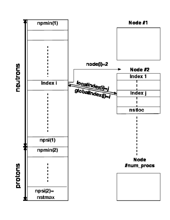
Figure 1: Storage arrangement of the single-particle wave functions. On the left the case for single-processor or OpenMP is shown, which for the case of distributed memory under MPI is mapped to the individual processors as shown on the right. Note that each node will have its own values of nstloc and globalindex.

If the code is run in parallel (MPI) on several nodes, only nstloc single-particle wave functions are stored on a given node, where nstloc may vary. Pointers are then defined to indicate the relationship between the local index and that in the global array of wave functions. For details see the section on parallelization.

There are a number of arrays containing the physical properties of the wave functions, such as the single-particle energy. The names start with sp_ and they are defined in module Levels. They are not split up in the parallel case, but on each node only the pertinent index positions are used.

2.7.6 Densities and currents

The various densities necessary for constructing the mean field are actually kept in separate arrays and can be output onto data files for later analysis (see subroutine write_densities). The dimensioning is (nx,ny,nz,2) with the last index referring to isospin for scalar densities, so that rho(:,:,:,1) is the neutron density and rho(:,:,:,2) the proton density. For vector densities there is an additional index with values 1 to 3 for the Cartesian direction, thus sdens(nx,ny,nz,3,2) containing the spin density in each direction for neutrons and protons.

Since it is often not necessary to keep the neutron and proton contributions separate, subroutine write_densities has the option of adding them up before output.

2.8 Initialization

A particular strength of the code is its flexible initialization. There are essentially three types of initialization, which can be selected through the input variable nof:

1. Harmonic oscillator: nof=0: this is applicable only to static calculations. The initial wave functions are generated from harmonic oscillator states with initial radii radinx, radiny, and radinz in the three directions. It is advisable to choose the three radii different to avoid being kept in a symmetric configuration for non-spherical nuclei. Note that this is a very simple initialization and has some defects; for example, the initial deformation is controlled more by the occupation of the oscillator states than by the radius parameters. This should eventually be replaced by, e. g., Nilsson wave functions.

   For this case the type of nucleus is determined by the input numbers nneut and nprot giving the number of neutrons and protons, while npsi can be used to add some unoccupied states (this sometimes leads to faster convergence).

2. Fragment initialization: nof>0: wave functions for a number nof of fragments are read in and positioned in the grid at certain positions. The wave functions are read from files produced by the static code with the file names given by the input filename, they are positioned at center-of-mass positions fcent and given am initial velocity controlled by fboost. The code determines the number of wave functions needed from these data files and also checks the agreement of Skyrme force and grid used. This initialization is used, e.g., for nuclear reactions (see Section 2.5.4).

   The number of fragments read in is arbitrary, but there are two special cases:

   • for nof=1 a single fragment is read in. This can be useful for initializing with static wave functions to study collective vibrations in a nucleus using the TDHF mode.

   • for nof=2 a special initialization can be done where the initial velocities are not given directly but computed from a center-of-mass energy ecm and an impact parameter b.

3. User initialization: a user-supplied routine user_init can be employed to set up the wave functions in any desired way. The only condition is that the index ranges etc. are set up correctly and the wave function array psi is filled with the proper values. It was found useful, e. g., to use initial Gaussians distributed in various geometric patterns for $\alpha$-cluster studies.

2.9 Restarting a calculation

Sometimes it is necessary to continue a calculation that was not run to the desired completion because of a machine failure or because the number of iterations or time steps was set too low. In such cases the last wave function file with name wffile, which is generated at regular intervals of mrest iterations or time steps, can be used to initialize a continuation. The program handles this in a simple fashion: if the logical variable trestart is input as TRUE, it sets up an initialization with one fragment (read from the initialization file) placed at the origin and with zero velocity. The only other modifications to the regular setup are then to take the initial iteration number and time from that file instead of starting at zero, as well as suppressing some unneeded initialization steps.

This flexible restart makes it possible to use a different grid for the continuation in the sense that the grid spacings must agree, but the new grid can be larger than the old one.

2.10 Accuracy considerations

The grid representation and solution methods introduced above depend on several numerical parameters. Their proper choice is crucial for the accuracy and speed of the calculations. In this Section, we want to briefly address the dependence on numerical parameters. An extensive discussion of grid representations and static iteration is found in [38].

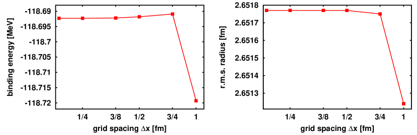
Figure 2: Binding energy (left) and r.m.s. radius (right) of ¹⁶O computed for the force SkI3 drawn as functions of grid spacing $\Delta x=\Delta y=\Delta z$. A logarithmic scale us used for $\Delta x$. The number of grid points has been chosen to keep the box size constant at $N_{x}\Delta x=24$ fm.

Figure 2 shows the sensitivity with respect to the grid spacings $\Delta x$, $\Delta y$, $\Delta z$. The trend is the same for both observables, energy and radius: The results have very high quality and change very little up to $\Delta x=$ 0.75 fm. They quickly degrade above that spacing. But even at $\Delta x=$ 1 fm, we still find an acceptable quality which suffices for most applications, particularly for large scale explorations. If high accuracy matters, $\Delta x\approx$ 0.75 fm should be chosen; not much is gained by going to even finer gridding. This holds for ground states and moderate excitations. High excitations and fast collisions may require a finer mesh. Note that the maximum representable kinetic energy is $E_{\mathrm{kin,max}}=(\hbar^{2}/2m)(\pi/\Delta x)^{2}$, which amounts to about 200 MeV for $\Delta x=$ 1 fm. The actual energies of interest should stay far below this limit. It is an instructive exercise to study uniform center-of-mass motion at various velocities to explore the limits of a given representation.

The number of grid points $N_{x}=N_{y}=N_{z}$ in the tests of Figure 2 were chosen such that the box size was the same in all cases. The actual choice of $N_{x}$ depends sensitively on the system, its size and separation energy. As a rule of thumb, the density decreases asymptotically as $\rho\propto\exp{(-2\sqrt{2m\varepsilon_{N}}r/\hbar)}$ where $\varepsilon_{N}$ is the single particle energy of the least bound state. One should aim for at least $\rho<10^{-8}$ at the boundaries.

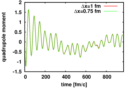
Figure 3: Time evolution of the quadrupole momentum for two different grid spacings $\Delta x=\Delta y=\Delta z$ and constant box size of 24 fm. The test case is ¹⁶O excited by an instantaneous boost computed with the force SkI3.

Figure 3 explores the effect of grid spacing for dynamics. Two different spacings are compared for a quadrupole oscillation following an instantaneous quadrupole boost. Practically no difference can be seen for the “safe choice” $\Delta x=$ 0.75 fm and the robust choice $\Delta x=$ 1 fm. Dynamical applications, oscillations and collisions, are in general less demanding and can be performed very well with $\Delta x=$ 1 fm. This is pleasing as dynamical calculations are usually much more costly than purely static ones.

There are two parameters regulating the static iteration according to Eq. (12), the damping energy e0inv and the step size x0dmp. e0inv should correspond to the depth of the binding potential. The overall step size x0dmp can be of order of one if e0inv is well chosen. Nuclear binding is very similar all over the chart of nuclei. This allows to develop one safe choice for nearly all cases. We recommend e0inv$\approx 100$ MeV together with x0dmp$\approx 1/2$, reducing the latter slightly if convergence problems appear. Of course, a few percent in iteration speed my be gained by fine-tuning these parameters for a given case, but this is not worth the effort unless large scale surveys for a given class of nuclei and forces are planned.

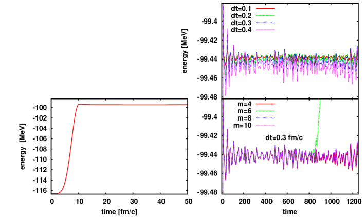
Figure 4: Time evolution of the binding energy of ¹⁶O after an excitation by a soft sin² pulse of width 20 fm/c computed for the force SV-bas [24] with a grid spacing $\Delta x=0.75$ fm and box size of 24 fm. Results are shown for different sizes of time step dt and different order of Taylor expansion m of the exponential evolution. The left panel shows the full evolution from ground state energy to the excited energy. The right panels concentrate on the times after the pulse is over in a narrower energy range relevant for this excitation.

The time stepping using the exponential propagator has the two parameters, step size dt and order mxp$=m$ of the Taylor expansion (18) of the exponential. Intuitively, one expects that small dt and large mxp improve the quality of the step. An efficient stepping scheme, however, looks for the largest dt and smallest mxp which still provide acceptable and stable results. It is hard to give general rules as good working values for the parameters depend on all details of the actual calculation: gridding, nuclei involved, excitation energy, and kind of excitation.

Figure 4 demonstrates the dependence of a typical dynamical evolution on these time-stepping parameters. We consider a time interval up to 1260 fm/c which is a long time for heavy-ion collisions and just sufficient for a spectral analysis of oscillations [41]. The excitation is done by a soft sin² pulse of finite extension in time. The energy increases during the initial excitation phase, as can be seen from the left panel in the figure. After the external pulse is over, energy conservation holds, which is nicely seen at plotting resolution in the left panel. Normalization should be conserved at all times. Both conservation laws serve as tests for the time step. Norm is conserved up to at least six digits for all cases and times shown in Figure 4. The energy is more critical. The right panels show the energy in a small window around the final energy after the excitation phase is over. The right lower panel shows a variation of the Taylor order $m$ for fixed time step. The most prominent effect is the sudden turn to catastrophic failure for $m=6$. In fact, propagation by approximate exponential evolution explodes sooner or later in all cases. The art is to extend the stable interval by a proper choice of the stepping parameters. It is plausible that the cases with $m>6$ maintain stability longer because the exponential is better approximated. It is surprising that $m=4$ is also stable over the whole time interval. There seem to be subtle cancellations of error going on. Considering the stable signals, we see very little differences between the cases. One may generally be happy with low $m$. It is mainly stability demands which could call for larger $m$. Note that this is not a generic result. Stability for a given test case should be checked once in a while and particularly before launching larger surveys.

The right upper panel in Figure 4 shows results for different dt (as we have seen, the $m$ values are not important as long as we achieve stable results). Here we see a clear dependence on the step size. The energies remain constant in the average. But there are energy fluctuations and these depend sensitively on dt. Smaller dt yields smaller fluctuations. As far as one can read off from the figure, the amplitude of the fluctuations shrink $\propto$dt². It depends on the intended analysis to which level of precision the time evolution should be driven. A value of dt$\approx$ 0.4 fm/c will be acceptable in most cases because the average trend remains far smaller than the fluctuations. Here also it must be emphasized that this is not a generic number. Forces with lower effective mass (SV-bas has $m^{*}/m=0.9$) are more demanding and usually require smaller dt. On the other hand, running propagation without the spin-orbit term allows even larger time steps because the spin-orbit potential is the most critical piece in the mean-field Hamiltonian. The mix of $\mathbf{p}$ and $\mathbf{r}$ imposes high demands on the numerical representations. We again strongly recommend running a few tests when switching forces or excitation schemes.

3 Code structure

The code is completely modularized to provide as large a degree of encapsulation as possible in order to ease modification. Most modules read their operating parameters from an associated NAMELIST and have their local initialization routines. In addition, a modern style of programming is used that employs a minimum number of local variables and streamlined array calculations that make the code lines very close to the physical equations being solved.

Here we give a brief overview over the modules and their purpose. There is a comprehensive manual supplied with the electronic version that gives a detzailes description of all modules. The source files containing the modules have the same names, but all in lower case, with an extension of .f90. The higher-level modules are:

Main program: It calls initialization routines, sets up the initial wave functions using either harmonic oscillator states or reading wave functions of static Hartree-Fock solutions from given input files (module Fragments). It then calls either statichf from module Static or dynamichf from module Dynamic to run the calculation.

Static: This contains the code for the static iterations statichf and the subroutine sinfo to generate output of the results.

Dynamic: runs the dynamic calculation in dynamichf and generates output in tinfo. Also controls the inclusion of an external excitation implemented in module External.

Densities: calculates the densities and current densities by summing over the single-particle states.

Meanfield: contains the central physics calculation: the computation of the components of the mean field (subroutine skyrme) and the application of the single-particle Hamiltonian to a wave function (subroutine hpsi).

Coulomb: calculation of the Coulomb potential.

Energies: calculation of the total energies and its various contributions.

External: calculation of the action of an external potential or initial collective boost of the wave functions.

Pairs: Implementation of the pairing correlations in the BCS approximation.

Moment: calculation of moments and deformation parameters for the bulk density.

Twobody: attempts to divide up the system into two separated nuclei and to calculate their properties and relative motion.

The lower-level supporting modules are:

Params: general parameters used throughout the code.

Forces: defines parameters of the Skyrme force and the pairing interaction and constructs them according to input.

Grids: defines everything associated with the numerical grid and sets it up.

Levels: definition of the single-particle wave functions and elementary operations on them such as derivatives.

Fragments: controls the reading of static wave functions from precomputed data and setting them up in the grid.

Inout: contains the subroutines for I/O of wave functions and densities.

Trivial: defines some very basic operations on wave functions and densities.

Fourier: sets up the transform plans for the FFTW3 package to calculate Fourier transforms of wave functions and densities.

Parallel: This comes in two versions. The source file parallel.f90 contains the routines to handle MPI message passing, while sequential.f90 sets up essentially dummy replacements for sequential or OpenMP mode.

User: contains a sample user initialization code which can be used as a template for more complicated setups.

4 Parallelization

For both OpenMP [46] and MPI [47] the code can be run in parallel mode. Parallelization for the static mode works in OpenMP but not in MPI: the reason is in the orthogonalization step which is not easily amenable for distributed-memory parallel computation. This should be worked on in the future.

MPI and OpenMP can be used jointly if there are computing nodes with multiple processors.

In both cases parallelization is done over the wave functions. The code applies the time-development operator or the gradient iteration, which use the fixed set of mean-field components, to each wave function, and this can naturally be parallelized. Computing the mean fields and densities by summing up over single-particle wave functions is also easily parallelizable.

The library FFTW3 [48] itself can also run on multiple processors in parallel. This can be used in addition to OpenMP or MPI, but was found to be helpful only in the sequential version of the code.

4.1 OpenMP

The application of the subroutine tstep for propagating one wave function for one time step, and of add_densities for adding one wave function’s contribution to the mean fields is done in parallel loops. The only complicating factor is that the densities, being accumulated in several subsets, must be kept separate using the REDUCTION(+) clause of OpenMP. The summation cannot be done internally in add_densities, because for the half time step the wave functions are immediately discarded after adding their contribution to the densities to avoid having to store the full set at half time. Thus only the combined tstep-add_densities loop should be parallelized.

The OpenMP program version can be compiled using the appropriate compiler option. A separate Makefile.openmp is provided which just contains the -fopenmp option for the GNU compiler. The number of parallel threads is not set by the code: the user should set the environment variable OMP_NUM_THREADS to the desired number.

4.2 MPI

In principle MPI uses the same technique as OpenMP, parallelizing over wave functions. In this case, however, each node contains only a fraction of the wave functions. This has several consequences:

1. The time-stepping of the wave functions can be done independently on each node, but requires that the densities are broadcast to all nodes after each half or full time step by summing up partial densities from the nodes in subroutine collect_densities.

2. The other calculation that uses wave functions directly is that of the single-particle properties. These are calculated on each node for the wave functions present on that node and then collected using subroutine collect_sp_properties.

3. Only one node must be allowed to produce output. This is regulated by choosing node #0 and setting the flag wflag.

4. The saving of the wave functions is done in the following way: Node zero writes a header file containing the job information on file wffile, then each node writes a separate file wwfile.001, wwfile.002, and so on up to the number of nodes. This avoids having to collect the wave functions on one node.

5. Using these parallel output files as fragment initialization or restart files is handled so flexibly that they can be read into a different nodal configuration or even a sequential run.

The MPI version needs the appropriate compiler and linker calls for the system used. The sequential or OpenMP versions are obtained simply by linking with sequential.f90 instead of parallel.f90, which replaces the MPI calls with a set of dummy routines and sets up the descriptor arrays for the wave function allocation in a trivial way.

The Makefile.mpi shows the procedure; in practice systems differ considerably and the user should look up the compilation commands for his particular system.

5 Input description

All the input is through NAMELIST and many variables have default values. The NAMELISTs should be in this file in the order in which they are described here, any NAMELIST not used for a particular job may be omitted or left in the input file, in which case it is ignored. The input is from standard input, so if the data are prepared in a file inputdata and the large output listing is to go into output, the code should be run using, e. g.,

./sky3d.seq␣<␣inputdata␣>␣output

5.1 Namelist files

files This NAMELIST contains names for the files used in the code. They are defined in module Params and are:

wffile: file to contain the static single-particle wave functions plus some additional data. This can be used for fragment initialization or for restarting a job. Default: ’none’, i. e., nothing is written.

converfile: contains convergence information for the static calculation. Default: conver.res.

monopolesfile: contains moment values of monopole type. Default: monopoles.res.

dipolesfile: contains moment values of dipole type. Default: dipoles.res.

quadrupolesfile: contains moment values of quadrupole type. Default: quadrupoles.res.

momentafile: contains components of the total momentum. Default: momenta.res.

energiesfile: energy data for time-dependent calculations. Default: energies.res.

spinfile: time-dependent total, orbital, and spin angular-momentum data as three-dimensional vectors.

extfieldfile: time dependence of expectation value of the external field.

5.2 Namelist force

force This defines the Skyrme force to be used. In most cases it should just use two input values:

name

: the name of the force, referring to the predefined forces in forces.data.

pairing

: the type of pairing, at present either NONE for no pairing, VDI for the volume-delta pairing, or DDDI for density-dependent delta pairing. The pairing parameters are included in the force definition. Note that the pairing type must be written in upper case.

There is also the possibility for inputting a user-defined force; this is described in detail with module Forces in the online technical documentation.

5.3 Namelist main

main This contains general variables applicable to both static and dynamic mode. They are mostly defined in module Params.

tcoul:

determines whether the Coulomb field should be included. Default is true.

trestart:

if true, restarts the calculation from wffile. Default is false.

tfft:

if true, the derivatives of the wave functions, but not of the densities, are done directly through FFT. Otherwise matrix multiplication is used, but with the matrix also obtained from FFT. Default is true.

mprint:

control for printer output. If mprint is greater than zero, more detailed output is produced every mprint iterations or time steps on standard output.

mplot:

if mplot is greater than zero, a printer plot is produced and the densities are dumped every mplot time steps or iterations. Default is 0.

mrest: if greater than zero, a wffile is produced every mrest iteration or time step. Default is 0.

writeselect

: selects the output of densities by giving a string of characters choosing them (see subroutine write_densities for details. Default is ’r’, i. e., only the density is written.

write_isospin

: determines whether the densities should be output isospin-summed (false) or separately for neutrons and protons (true). Default is false.

imode

: selects a static imode=1 or dynamic imode=2 calculation.

nof

: (number of fragments) selects the initialization. nof=0: initialization from harmonic oscillator, only for the static case; nof<0: user-defined initialization by subroutine init_user in module User; nof>0: initialization from fragment data as determined in NAMELIST fragments.

5.4 Namelist grid

grid This defines the properties of the numerical grid.

nx, ny, nz

: number of grid points in the three Cartesian directions. They must be even numbers.

dx, dy, dz

: spacing between grid points in fm. If only dx is given in the input, all three grid spacings become equal. The grid positions are then set up to be symmetric with the coordinate zero centrally between point number nx/2 and nx/2+1.

periodic

: chooses a periodic (true) or isolated (false) system.

5.5 Namelist static

static These input variables control the static calculations.

tdiag:

if true, there is a diagonalization of the Hamiltonian during the later (after the 20th) static iterations. This 20 is hard coded in static.f90. Default is false.

tlarge:

if true, during the diagonalization the new wave functions are temporarily written on disk to avoid doubling the memory requirements. Default is false.

nneut, nprot:

The numbers of neutrons and protons in the nucleus. These are used for the harmonic-oscillator and user initialization.

npsi:

the numbers of neutron (npsi(1)) and proton (npsi(2)) wave functions actually used including unfilled orbitals. Again, useful only for harmonic-oscillator or user initialization.

radinx, radiny, radinz:

the radius parameters of the harmonic oscillator in the three Cartesian directions, in fm.

e0dmp:

the damping parameter. For its use see subroutine setdmc. The default value is 100 MeV.

x0dmp:

parameters controlling the relaxation. The default value is 0.2. In special cases it may be desirable to change this to accelerate convergence.

serr:

this parameter is used for a convergence check. If the sum of fluctuations in the single-particle energies, sumflu goes below this value, the calculation stops. A typical value is 1.E-5, but for heavier systems and with pairing this may be too demanding.

5.6 Namelist dynamic

dynamic These are variables controlling the dynamic (TDHF) calculation.

nt

: number of time steps to be run.

dt

: the time step in fm/c. A standard value is of the order of 0.2 to 0.3 fm/c, it depends somewhat on the value of mxpact. If the combination of these two is not good enough, the calculation becomes unstable after some time, in the sense that the norm of the wave functions and the energy drift off and can diverge (see Sect. 2.10).

mxpact

: the order of expansion for the exponential time-development operator. The predictor (trial) step calculation uses mxpact/2 as the order. For more information see Sect. 2.10.

rsep

: termination condition. If the final state in a two-body reaction is also of two-body character, the calculation is terminated as soon as the separation distance exceeds rsep. Units: fm. No default. The purpose of this variable is to prevent the calulation of continuing into meaningless configurations, like crossing of the boundary.

texternal

: indicates that an external perturbing field is used. In this case the namelist extern must be present. Default: false.

5.7 Namelist extern

extern The variables read here describe the external field that is applied to get the nucleus into a collective vibration. Details can be found in the description of module External. It is read only if the parameter texternal read in namelist dynamic is true.

ipulse

: the type of pulse applied. For ipulse=0 the wave function is multiplied with a phase factor that produces an initial excitation.For ipulse=1 a Gaussian time dependence is used, for ipulse=2 a $\cos^{2}$ one. Default: 0. Details are given in Eqs. (9d) and (9e).

isoext

: isospin character of the excitation. If this is zero, protons and neutrons are exited in the same way. For a value of 1, they behave oppositely but with a coupling that leaves the center-of-mass invariant. Default: 0.

tau0, taut

: time at which the excitation field reaches its maximum, and width of the pulse. No defaults.

omega

: if this is nonzero, the time-dependence of the external field gets an additional cosine factor with frequency omega.

radext, widext

: radius and width of a Woods-Saxon-type cutoff factor in radius for the external field. Defaults: 100 fm and 1 fm, which practically implies no damping. Definition in Eq. (9b).

amplq0

: amplitude for quadrupole excitation of the $Q_{20}$ type. Defined as usual with respect to the $z$-axis.

5.8 Namelist fragments

fragments The variables in this namelist control fragment initialization for the case of nof>0. Most quantities are dimensioned for the fragments and we indicate this by index “i” in the following.

filename(i)

: the name of the file containing the wave functions of fragment i.

fcent(1:3,i)

: initial position of fragment i given as three Cartesian coordinate values in fm. The position must be such that the complete fragment grid fits inside the new computational grid.

fix_boost

: used only for the two-fragment case. if this logical variable is TRUE, the initial velocities are calculated from the fboost values; otherwise from the relative motion quantities ecm and b.

fboost(1:3,i)

: the initial boost of the fragment in the three Cartesian directions. It is given as the total kinetic energy in each direction in MeV, with the sign indicating positive or negative direction. Thus SUM(ABS(fboost(:,i))) is the total kinetic energy of fragment i.

ecm, b

: center-of-mass kinetic energy in MeV and impact parameter in fm. Used only if fix_boost is FALSE. These are the values at infinite distance and are corrected using Rutherford trajectories (assuming spherical nuclei) for initialization at the finite distance given by the fcent coordinates.

5.9 Namelist user

user This namelist is read only if needed for user initialization (see module User). Its contents depend on the specific user initialization and the only thing to be said here is that it should appear last in the input file. Since the namelist is defined and used only in module User, its name can also be changed arbitrarily, of course.

6 Output description

The code produces a number of output files containing various pieces of information. The bulky observables, such as densities or currents, are selectively output at certain time steps into special binary output files nnnnnn.tdd), where nnnnnn indicates the iteration or time step number. These files can then be used for further analysis or converted to be used as input in visualization codes. Examples of this are found among the utility codes provided.

The complete set of wave functions is saved at regular intervals of mrest iterations or time steps. Because this leads to large storage requirements, only the last such file in a run is kept. It can be used for restarting the calculation or for inputting fragment wave functions for initializing another calculation.

In MPI mode the wave functions are distributed over several files, each containing only those present on a specific processor. An additional header file contains the remaining information and can be used to read the wave functions even on a different processor configuration.

Aside from these binary files there are a number of text files. The *.res files contain one line for each time step or iteration where output is triggered according to the value of mprint. There is an explanatory header line in these that has a leading ’#’, so that is treated as a comment by gnuplot — thus gnuplot can be used immediately to plot the behavior of any one column of numbers, i. e., the dependence of a physical quantity on iteration or time. In addition more complicated output is printed on standard output, which can be redirected into a file using shell redirection.

The names of the output files can be adjusted using input variables as listed in Section 5.1, so that the files are here denoted by the default names given there. The *.res files are relatively small, so that no mechanism was implemented to suppress them.

6.1 File conver.res

This is produced in sinfo only in the static calculation and its purpose is to give a quick impression of the convergence behavior. The numbers given in each line are the iteration count, the total energy in MeV, the relative change in energy from one iteration to the next, the average uncertainties in the single-particle energies efluct1 and efluct2, the root-mean-square radius in fm and finally the deformation parameters $\beta$ and $\gamma$ (see Section 2.6.1). The latter give an impression as to where the nuclear shape is ending up.

For the judging of convergence, the efluct values are more important than the change in total energy, since the energy can remain constant while the wave functions still change considerably.

6.2 File monopoles.res

At present this file is generated in subroutine moment_shortprint, but only in the dynamic mode. It contains the time, the neutron, proton, and total root-mean-square radii, and the difference of neutron minus proton root-mean-square radii.

6.3 File dipoles.res

This file is produced both in the static and dynamic calculations in subroutines sinfo and tinfo. It contains the iteration or time step number followed by the three components of the center of mass vector $\vec{R}$ and those of the difference of proton minus neutron center-of-mass vectors $\vec{R}^{(T=1)}$, both in fm, for the definition see Eq. (21a). The first of these is useful as a check to see whether the center of mass drifts off during the calculation, while the second vector may be useful to look at proton vs. neutron vibrations.

6.4 File quadrupoles.res

This is also generated in moment_shortprint and thus only in dynamic mode. It contains the Cartesian quadrupole moments (21b) for neutrons, protons, and the full mass distribution followed by the expectation values of $x^{2}$, $y^{2}$, and $z^{2}$ for neutrons and protons, all in fm².

6.5 File energies.res

This is the important monitoring file for the dynamic calculation. It is written in subroutine tinfo and each line contains the simulation time, the number of neutrons and protons in the system (these should be constant, so this is a stability check), the total energy (again, this should be conserved), the total kinetic energy, and finally the collective energy ecoll separately for neutrons and protons. Units for the energies are all MeV.

6.6 Standard output

This contains all the additional information that in most cases is not needed directly for further processing in, e. g., graphics programs. If it should be found necessary to utilize some data from this file, it is in most cases easy to use grep or a scripting language like PERL or PYTHON to extract the necessary data. Of course the code can also be modified to produce additional output files.

The initial part of the output essentially echoes all the data from the NAMELISTs in tabular form, to enable checking the correctness of input data. In the case of fragment initialization this is more involved and is discussed below for the dynamic case, since it is not so common for static calculations.

In general the layout of the information is compact with sequences of “*” characters to provide separation between input groups as some guidance for the eye.

6.6.1 Static calculation

The code first prints the current iteration number. Iteration “0” refers to the state before iterations are started, for the later iteration numbers, the information refers to the end of the iteration.

The an overview of the various energy contributions is printed: the first part is similar to what in in file conver.res, while a second list shows the energies calculated from the density functional and split up for the various contributions.

Next there is a simple printer plot of the density distribution in the $(x-z)$-plane. This is often quite helpful, since it shows what is going on in the calculation without the need to start a graphics program, which requires converting the data first.

Next there is a listing of single-particle states. For each state this shows its parity, occupation probability wocc (which is called $v^{2}$, as it is interesting mostly in the pairing case), the energy fluctuations sp_efluct1 and sp_efluct2, the norm, the kinetic and total energies of the state, and finally the expectation values of the three components of the orbital and spin angular momentum, respectively.

Finally a summary of some integrated quantities is given, separately for neutrons, protons, and all nucleons: the particle number, the root-mean-square radius, quadrupole moment, and the average of the coordinates squared, followed by the center-of-mass components.

Then iterations continue and only one line is printed for each, as this may be quite slow and it is important to be able to check progress while the code is running. After mprint iterations the detailed information is repeated.

6.6.2 Dynamic calculation

After echoing the parameters for the dynamic calculation, the fragment definitions are given and all the resulting information is printed: the computed boost values in case of twobody initialization, the properties of the single-particle states read in, including which index in the fragment file is transferred to which index in the total set of wave functions.

In case of an external field, the input data is also echoed in a detailed form.

The time stepping starts and detailed output is produced every mprint steps at the end of the time step. Much of it is similar to the the static case, so only the differences are pointed out.

Because in the dynamic case the situation can have a general three-dimensional character, the full information on the quadrupole tensor (21b) is printed, separately for the neutron, proton, and total mass distributions. The three eigenvalues and associated normalized eigenvectors are given, followed by Cartesian and polar deformation parameters $a_{0}$, $a_{2}$, $\beta$, and $\gamma$, as defined in Section 2.6.1.

The separation of the two fragments and its time derivative is printed next and repeated every time step, as examining these quantities is meaningful only with more frequent sampling.

The energy information is shortened by omitting the quantities not of interest in the dynamic case. After the printer plot the results of the two-body analysis are given (for the meaning of the various quantities see module Twobody in the online documentation. The Section on “collision kinematics” shows the mass, charge, position, and kinetic energy of the two fragments. It should be kept in mind that the two-body analysis is only valid if the reaction plane is the $(x-z)$-plane and the results printed may not be useful if the physical situation is not of two-body nature but the code does not recognize that.

The single-particle property list and the integrated quantities are as in the static case, but the energy fluctuations are omitted.

The next time step is then indicated and the fragment separation data are printed for every time step until after mprint steps the full output recurs.

7 Utilities

A set of short programs is designed to help with further processing of output from the code. The currently available set is described here.

Most of these routines contain a loop to input a file name from the terminal. If it is desired to do this in a loop over a set of files, a simple trick can be used: generate a list of file names using, e. g.,

ls -1 *.tdd > list

and then execute the program with “list” as input, e. g.,

./fileinfo < list

For Tdhf2Silo a script convert is provided that handles this (see below). It can easily be adapted to the other utilities and must be stored in the same directory as the executable utility program itself in order for the dirname command to work properly.

7.1 Fileinfo

This is a short program to print information about binary files generated by Sky3D. It takes the name of either a *.tdd or a wave function file as input and prints out essentially all the information contained in the header. It can be compiled simply by executing

gfortran -o fileinfo fileinfo.f90

7.2 Inertia

This is intended as an example of an analysis code reading *.tdd files and doing some computation, which can be used as a model for doing similar things. It illustrates looking for the desired field in the file and taking into account whether it is stored as a total density or isospin-separated. Being given a filename as input, it reads the density and calculates the inertia tensor to print all its 9 components. Compile it using

gfortran -o Inertia Inertia.f90

7.3 Cuts

This utility reads the density from a file nnnnnn.tdd file and produces output files named nnnnnnrxy.tdd, nnnnnnrxz.tdd, and nnnnnnryz.tdd, which contains two-dimensional cuts through the system in the $(x,y)$, $(x,z)$, and $(y,z)$ plane, respectively. The cuts are evaluated at the origin for the third coordinate by averaging the two neighboring planes.

These data files are written in such a format that they can be read by gnuplot for use in its commands for 2-dimensional plotting.

This program is intended again as a template that can be modified for other applications.

7.4 Overlap

This is a code to calculate the overlap of two Slater determinants. Given the names of two wave function files (which must contain compatible data: dimensions, force, etc.) it reads the wave functions, generates the matrices of overlaps between one set and the other separately for neutrons and protons, and then calculates the determinant of each, which is the overlap between the two Slater determinants. It prints some summary information: distance between the centers of mass of each set, minimum and maximum diagonal elements, maximum absolute value of off-diagonal elements, and finally the overlaps for protons and neutrons as well as their product.

This code uses subroutines from LINPACK (stored at NETLIB.ORG), which are included in the file det.f with appropriate copyright. It can be compiled using

gfortran -o overlap overlap.f90 det.f.

7.5 Tdhf2Silo

This program is quite complicated. It reads a set of *.tdd files and converts them into Silo files. Silo is a library for handling scientific datasets developed at Lawrence Livermore National Laboratory (https://wci.llnl.gov/codes/silo/index.html). This is the most appropriate library to use in conjunction with the LLNL graphics visualization tool VisIt (https://wci.llnl.gov/codes/visit/home.html), which was found to be highly suitable for plotting Sky3D results and producing movies. The conversion code is quite flexible in that it decides what to produce for the different field types: isospin-summed or not, vector or scalar. They are given appropriate names for Silo with suffixes p and n for protons and neutrons, and x, y, z for the vector components. In the case of vector fields a variable containing the vector definition is also written so that the field can be plotted immediately as a vector field in VisIt.

If the user wants another dataset handling method, the code should be readily adaptable to other libraries. VisIt itself has many ways of importing data, but of course there also alternative 3D visualization systems.

8 Running the code

8.1 Compilation and linking

To produce executable files the code comes with several Makefiles. The standard Makefile produces a sequential code sky3d.seq, the file Makefile.openmp a parallel code using OpenMP, while Makefile.mpi should produce an MPI distributed system code.

The Makefiles are written for the gfortran compiler and the commands and options must be adapted if other compilers are used. The user may also have to modify the library names and execution of the code under MPI will require consulting the local documentation or system administrator.

No attempt was made to select the compiler and linker options optimally for speed, since experience has shown that optimization at the cutting edge is highly time-dependent. Thus users should do some speed tests before embarking on major calculations.

8.2 External libraries needed

The LAPACK library is used in the code to supply the routines ZHBEVD and DSYEV. LAPACK should be installed in most scientific computing centers; if not, the files can be obtained from www.netlib.org and just be added as additional source files to the code. Note that a complete set of routines called by these two subroutines must be downloaded.

The other external routine library that is used is FFTW3. Again, it will be preinstalled in most systems. If not, there are two possibilities:

1. Download the source code from www.fftw.org and compile the library yourself. In our experience this worked smoothly. The generated library can be installed in a system library directory or kept in a user account. In the latter case the use of -lfftw3 in the makefiles does not work anymore and the full path name of the library file must be given.

2. Replace it by another FFT routine. This requires quite a bit of work: FFTW organizes its calls around “plans”, which describe a set of operations to be done on the three-dimensional arrays. In init_fft quite sophisticated plans are set up to, for example, transform in the y-direction for all x- and z-values.This means that all calls to subroutines beginning with dfftw have to be examined and possibly replaced by loops over one-dimensional FFT transforms. This should be relatively straightforward, but there are two more important points to consider: 1) normalization differs between FFT codes. For FFTW transformation followed by inverse transformation multiplies the original data by nx*ny*nz and this factor is taken into account in several places. 2) For the non-periodic case the Fourier transform in the Coulomb solver uses doubled dimensions in all three directions. Some FFT codes have an initialization that sets up the transformation factors depending on the dimension; in such cases the initialization may have to be repeated.

8.3 Running with OPENMP

The OPENMP version can be compiled using the file Makefile.openmp, which produces an executable sky3d.omp. The main difference to the sequential makefile is the addition of an openmp compiler option. Since this depends on the compiler used, it may have to be modified. For gfortran the option is -fopenmp, while for Intel Fortran it is simply -openmp.

For controlling the running of the code the user should set the environment variable OMP_NUM_THREADS to the number of parallel threads to be used (usually the number of processors). In addition it may be necessary to set OMP_STACKSIZE. The two parallel loops in dynamichf need to store all the density fields in parallel, and the second loop adds ps4 to that. Taking into account vector fields and isospin, a total of 24 threedimensional COMPLEX(8) fields need to be stored, amounting to nx*ny*nz*24*16 bytes, which is the stack size needed.

8.4 Running under MPI

The situation for MPI is a bit more complex than for OPENMP, so that the file Makefile.mpi will almost certainly have to be modified. One crucial difference to the other makefiles is that the module Parallel is now generated from the source file parallel.f90. In addition the compilation commands have to be adapted; something like mpif90 will be needed but is installation dependent. In addition a command like mpirun will be needed for execution; the user is advised to consult local documentation.

8.5 Required input

Here it is just summarized what input is needed for a static or dynamic calculation. A full description can be found with the documentation for the NAMELISTs.

8.5.1 Static calculation

The NAMELISTs needed are, in that order:

files, force, main, grid, static. In addition, if initialization is from fragments, fragments, and for user initialization possibly user (only if the user initialization requires input).

8.5.2 Dynamic calculation

The NAMELISTs needed are, in that order:

files, force, main, grid, dynamic, For external field excitation extern, and in all cases fragments.

8.6 Test cases

To allow checking the proper behavior of the code, we provide three test cases exercising different functions: a static calculation for the ground state of ¹⁶O, a dynamic calculation using an external excitation to stimulate a giant resonance in ¹⁶O, and finally a sample deep-inelastic collision of two ¹⁶O nuclei. The test cases directory contains a more detailed description of these cases and what to look for principally in the results.

9 Caveats concerning the code

The user should be aware of the limitations of the code in various respects but also note some less straightforward procedures for improving accuracy in certain cases.

9.1 Static calculations

Since the main use of the code is expected to be in time-dependent calculations, the static part is less highly developed. The omission of all symmetry restrictions, while very useful for innovative applications with time-dependence, can cause some problems in the static case.

1. The spin is not aligned along a fixed direction. Since for even-even nuclei Kramers degeneracy operates, two degenerate levels will mix in an uncontrolled way to produce an arbitrary spin alignment. This can be remedied by diagonalizing the spin operators in such a two-level subspace.

2. The center of mass may move away from the origin during the iterations. This is typically a very small effect and will be corrected when the wave functions are placed at a given position in the dynamic initialization. The calculation of observables, however, should always use coordinates relative to the real center of mass.

3. In very heavy nuclei sometimes even a rotation was seen, as the reoccupation of high-lying levels can change the geometric orientation. If this is a serious problem, constraints should be introduced or another code used for the static calculation.

4. The harmonic oscillator initialization can be quite deficient for heavier nuclei. It is planned to develop a Nilsson-model alternative; meanwhile in case of problems the use of wave functions from axial or symmetry-restricting codes could be implemented by generating a wave function file from such results. Since this will involve interpolation, a number of static iterations should then be performed using the present code to improve stability.

9.2 Dynamic calculations

Here it is important what the required accuracy will be. Most exploratory calculations will not pose high accuracy demands. There are several possible ways in which accuracy can be improved if needed:

1. The initial configuration may be improved. If the fragment nuclei are not situated at grid points, one should run a number of static iterations with each fragment situated alone in the new grid.

2. If the fragments are deformed, the energy estimate from the Rutherford trajectory will not be reliable; in this case it is recommended to run a number of dynamic iterations, observe the change in relative distance, and then correct the boost energies to match the correct velocity of relative motion.

10 Modifying the code

Since the code was developed with a view for easy modification, in this Section we give some advice on how to add new things to it and how to run simulations.

10.1 Modifying the Skyrme force

The code comes with a quite large database of Skyrme force parametrizations together with appropriate pairing parameters built in. This is certainly useful to avoid mistakes in the input by having to indicate only the name of the force. Still there will be a need to add new forces and even forces with a different density functional to it, for which we suggest three different approaches.

10.1.1 Direct parameter input

If a specific parametrization is not expected to be a permanent addition to the code, for example if one or several parameters are varied to study the sensitivity of the results to specific parts of the density functional, the best way is to use the facility for giving the parameters directly in the input. This is triggered by using some force name that is not in the database, in which case the routine expects all parameters to be given in NAMELIST forces.

10.1.2 Expanding the database

At present the database of forces is contained in the file forces.data as a long initialization statement. This has the advantage of readability and avoids having to make a database file accessible in every directory used for code applications.

So a new force which will be used more permanently can be added simply by adding the appropriate lines in forces.data and increasing the number assigned to nforce accordingly. There is a slight danger that the total length of the list will exceed the 255 lines allowed by the Fortran standard; in this case either remove some outdated forces, remove the separation lines of all stars, or if there is still a problem, convert the initialization to DATA statements initializing a smaller number of forces in each case.

10.1.3 Adding new physics to the density functional

This can of course require a lot more modifications to the code. Generally speaking, such a new term will appear not only in the density functional, but also leads to new contributions in the single-particle Hamiltonian and may require new types of densities and currents. In addition, it will involve new force parameters. So in general the following steps will be needed:

1. Parameter definition: The new parameter can be added to the general Force type definition in forces.f90. This is the most logical and systematic way, but we recommend it only if the new physics is to be there permanently, since in this case the whole database has to be updated to give a default value — probably zero — to the new parameter for each existing force. The alternative is to leave this parameter as a separate entity, which can still be a module variable in Forces and be input using the same namelist. Derived parameters should also be calculated here.

2. New densities and currents: everything that can be defined directly as a sum over the occupied single-particle wave functions should be defined and calculated in module Densities. It should be a module variable and allocated during initialization similar to the densities already defined. Then the contributions of the different derivatives of the wave function can be accumulated separately as is done for the existing contributions.

3. Calculation of mean-field components: subroutine skyrme in module Meanfield is the place where the fields appearing in the single-particle Hamiltonian are calculated. The difference to module Densities is that wave functions are not involved directly, but only combinations and derivatives of the densities and currents need to be evaluated. The new fields should be defined and allocated and then calculated in subroutine skyrme. The handling of derivatives again can be imitated based on the existing terms.

4. Single-particle Hamiltonian: The additional contribution to the single-particle Hamiltonian must be calculated in subroutine hpsi of module Meanfield. Code has to added to calculate how the additional terms act on the input wave function pinn and the result has to be added to the output wave function pout. Again, for efficiency the spatial derivatives can be handled in separate loops.

5. Contribution to the energy: subroutine integ_energy in module Energies must include an additional contribution of the new term, which in this case means simply computing the expression for the energy functional. Probably it will be useful to add this up in some new variable (defined as a module variable), so that the contribution of the new term can be printed out together with the other contributions in subroutines sinfo of module Static or subroutine tinfo of module Dynamic, respectively.

6. Output of densities: it may be desirable to write out the new densities, currents, or mean-field contributions into the *.tdd files. To do that, subroutine write_densities in module Inout must be modified. A new letter to use for writeselect must be defined and selected in the SELECT CASE statement, and then depending on whether it is a scalar or a vector field, write_one_density or write_vec_density is called with a descriptive name given to the field.

   The complication that occurs here is that these writing routines assume isospin-dependent fields and output either isospin-separate or isospin-summed fields depending on the value of write_isospin. If the field has no isospin dependence, the statements used to output wcoul should be imitated.

   10.2 Analyzing the results in new ways

   The code provides quite a large number of physical observables in its output files. For new applications it may be necessary to look at additional ones. There are essentially two ways to implement this:

   1. If the new observable depends only on density and mean-field components, the easiest way is to use the *.tdd files, where if necessary more fields can be output by modifying the subroutine write_densities. As an example for reading the *.tdd files, we provide a code calculating the tensor of inertia among the utilities.

   2. It becomes more complicated if the wave functions have to be used. Here one possibility is to add a call to a user-written routine at the beginning of the static or dynamic loops, which then can use the array psi in any way desired. This may not be a good option if the calculations are lengthy and the analysis routine may have to be modified several times. In this case it is better to generate a new file name for the wffile each time write_wavefunctions is called, similar to the way it is done in write_densities, and to do the analysis by reading the wave function files.

References

- [1] A. L. Fetter, J. D. Walecke, Quantum Theory of Many-Particle Systems, McGraw-Hill, New York, 1971.
- [2] J. Maruhn, P.-G. Reinhard, E. Suraud, Simple models of many-fermions systems, Springer, Berlin, 2010.
- [3] R. M. Dreizler, E. K. U. Gross, Density Functional Theory: An Approach to the Quantum Many-Body Problem, Springer-Verlag, Berlin, 1990.
-
[4]
M. Bender, P.-H. Heenen, P.-G. Reinhard,
Self-consistent mean-field
models for nuclear structure, Rev. Mod. Phys. 75 (2003) 121.
URL http://dx.doi.org/10.1103/RevModPhys.75.121 - [5] P. Dirac, Exchange phenomena in the Thomas-Fermi-atom , Proc. Cambridge Philos. Soc. 26 (1930) 376.
- [6] G. E. Brown, Unified Theory of Nuclear Models and Forces, 3rd Edition, North-Holland, Amsterdam, London, 1971.
- [7] P.-G. Reinhard, E. Suraud, Introduction to Cluster Dynamics, Wiley, New York, 2004.
- [8] P. Bonche, S. E. Koonin, J. W. Negele, One–dimensional nuclear dynamics with time–dependent hartree–fock approximation, Phys. Rev. C 13 (1976) 1226–1258.
- [9] J. W. Negele, The mean–field theory of nuclear structure and dynamics, Rev. Mod. Phys. 54 (1982) 913–1015.
- [10] K. T. R. Davies, K. R. S. Devi, S. E. Koonin, M. R. Strayer, TDHF calculations of heavy–ion collisions, in: D. A. Bromley (Ed.), Treatise on Heavy–Ion Physics, Vol. 3 Compound System Phenomena, Plenum Press, New York, 1985, p. 3.
- [11] J. J. Bai, R. Y. Cusson, J. Wu, P.-G. Reinhard, H. Stöcker, W. Greiner, M. R. Strayer, Mean field model for relativistic heavy ion collisions, Z. Phys. A 326 (1987) 269–277.
- [12] H. Berghammer, D. Vretenar, P. Ring, Computer program for the time-evolution of a nuclear system in relativistic mean-field theory, Comp. Phys. Comm. 88 (1995) 293.
- [13] D. Vretenar, A. Afanasjev, G. Lalazissis, P. Ring, Relativistic hartree-bogoliubov theory: Static and dynamic aspects of exotic nuclear structure, Phys. Rep. 409 (2005) 101.
- [14] C. Simenel, P. Chomaz, Phys. Rev. C 68 (2003) 024302.
- [15] J. Maruhn, P.-G. Reinhard, P. Stevenson, I. Stone, M. Strayer, Phys. Rev. C 71 (2005) 064328.
- [16] A. S. Umar, V. E. Oberacker, Phys. Rev. C 71 (2005) 034314.
- [17] T. Nakatsukasa, K. Yabana, Phys. Rev. C 71 (2005) 024301.
- [18] Y. Hashimoto, K. Nodeki, A numerical method of solving time-dependent hartree-fock-bogoliubov equation with gogny interaction, arXiv:0707.3083.
- [19] A. Umar, V. Oberacker, Density-constrained time-dependent hartree-fock calculation of 16o + 208pb fusion cross-sections, Eur. Phys. J. A 39 (2009) 243. doi:10.1140/epja/i2008-10712-5.
-
[20]
N. Loebl, A. S. Umar, J. A. Maruhn, P.-G. Reinhard, P. D. Stevenson, V. E.
Oberacker,
Single-particle
dissipation in a time-dependent hartree-fock approach studied from a
phase-space perspective, Phys. Rev. C 86 (2012) 024608.
doi:10.1103/PhysRevC.86.024608.
URL http://link.aps.org/doi/10.1103/PhysRevC.86.024608 -
[21]
C. Simenel, Nuclear quantum
many-body dynamics, The European Physical Journal A 48 (11) (2012) 1–49.
doi:10.1140/epja/i2012-12152-0.
URL http://dx.doi.org/10.1140/epja/i2012-12152-0 - [22] J. Erler, P. Klüpfel, P.-G. Reinhard, Self-consistent nuclear mean-field models: example skyrme-hartree-fock, J. Phys. G 38 (2011) 033101. doi:10.1088/0954-3899/38/3/033101.
- [23] J. C. Slater, Phys. Rev. 81 (1951) 385.
-
[24]
P. Klüpfel, P.-G. Reinhard, T. J. Bürvenich, J. A. Maruhn,
Variations on a
theme by Skyrme, Phys.Rev. C 79 (2009) 034310,
http://www.arxiv.org/abs/0804.3385.
URL http://link.aps.org/doi/10.1103/PhysRevC.79.034310 -
[25]
P. Klüpfel, J. Erler, P.-G. Reinhard, J. A. Maruhn,
Systematics of collective
correlation energies from self-consistent mean-field calculations, Eur.
Phys. J A 37 (2008) 343, http://www.arxiv.org/abs/0804.340.
URL http://dx.doi.org/10.1140/epja/i2008-10633-3 - [26] J. Bartel, P. Quentin, M. Brack, C. Guet, H.-B. Håkansson, Towards a better parametrisation of skyrme forces: A critical study of the SkM force, Nucl. Phys. A 386 (1982) 79–100.
- [27] Y. M. Engel, D. M. Brink, K. Goeke, S. J. Krieger, D. Vautherin, Time-dependent hartree–fock theory with skyrme’s interaction, Nucl. Phys. A 249 (1975) 215–238.
- [28] E. Perlińska, S. G. Rohoziński, J. Dobaczewski, W. Nazarewicz, Local density approximation for proton-neutron pairing correlations: For malism, Phys. Rev. C 69 (1) (2004) 014316.
- [29] K. J. Pototzky, J. Erler, P.-G. Reinhard, V. O. Nesterenko, Properties of odd nuclei and the impact of time-odd mean fields: A systematic skyrme-hartree-fock analysis, Eur. Phys. J. A 46 (2010) 299. doi:10.1140/epja/i2010-11045-6.
- [30] D. Vautherin, D. M. Brink, Hartree–fock calculations with skyrme’s interaction I. spherical nuclei, Phys. Rev. C 5 (1972) 626.
- [31] P.-G. Reinhard, H. Flocard, Nuclear effective forces and isotope shifts, Nucl. Phys. A 584 (1995) 467–488.
- [32] K. Rutz, J. Maruhn, P.-G. Reinhard, W. Greiner, Fission barriers and asymmetric ground states in the relativistic mean field theory, Nucl. Phys. A 590 (1995) 680, http://www.arxiv.org/abs/nucl-th/9610037.
- [33] W. Greiner, J. A. Maruhn, Nuclear Models, Springer Verlag, New York, 1996.
- [34] P. Ring, P. Schuck, The Nuclear Many-Body Problem, Springer–Verl., New York, Heidelberg, Berlin, 1980.
- [35] P.-G. Reinhard, M. Bender, K. Rutz, J. Maruhn, An HFB scheme in natural orbitals, Z. Phys. A 358 (1997) 277, http://www.arxiv.org/abs/nucl-th/9705054.
- [36] M. Bender, K. Rutz, P.-G. Reinhard, J. Maruhn, Pairing gaps from nuclear mean–field models, Eur. Phys. J. A 8 (2000) 59, http://www.arxiv.org/abs/nucl-th/0005028.
- [37] P.-G. Reinhard, R. Cusson, A comparative study of Hartree-Fock iteration techniques, Nucl. Phys. A 378 (1982) 418.
- [38] V. Blum, G. Lauritsch, J. Maruhn, P.-G. Reinhard, Comparison of coordinate-space techniques in nuclear mean-field calculations, J. Comp. Phys. 100 (1992) 364.
- [39] W. H. Press, S. A. Teukolsky, W. T. Vetterling, B. P. Flannery, Numerical Recipes in C: The Art of Scientific Computing, 2nd Edition, Cambridge University Press, New York, 1992.
-
[40]
F. Calvayrac, E. Suraud, P.-G. Reinhard,
Spectral signals from
electronic dynamics in sodium clusters, Ann. Phys. (N.Y.) 255 (1997) 125.
URL http://dx.doi.org/10.1006/aphy.1996.5654 -
[41]
P.-G. Reinhard, L. Guo, J. A. Maruhn,
Nuclear giant resonances
and linear response, Eur. Phys. J. A 32 (2007) 19,
http://www.arxiv.org/abs/nucl-th/0703044.
URL http://dx.doi.org/10.1140/epja/i2007-10366-9 - [42] P.-G. Reinhard, From sum rules to RPA: 1. nuclei, Ann. Phys. (Leipzig) 504 (1992) 632.
-
[43]
N. Loebl, J. Maruhn, P.-G. Reinhard,
Equilibration in
the time-dependent hartree-fock approach probed with the wigner distribution
function, Phys. Rev. C 84 (2011) 034608.
doi:10.1103/PhysRevC.84.034608.
URL http://link.aps.org/doi/10.1103/PhysRevC.84.034608 - [44] P. Bonche, B. Grammaticos, S. E. Koonin, Three-dimensional time-dependent hartree-fock calculations of and fusion cross sections, Phys. Rev. C 17 (1978) 1700.
-
[45]
L. Guo, P.-G. Reinhard, J. A. Maruhn,
Conservation
properties in the time-dependent Hartree Fock theory, Phys. Rev. C 77
(2008) 041301, http://www.arxiv.org/abs/0804.2127.
URL http://link.aps.org/doi/10.1103/PhysRevC.77.041301 - [46] B. Chapman, G. Jost, R. van der Pas, Using OpenMP, MIT Press, Cambridge, 2008.
- [47] MPI: A Message-Passing Interface Standard, Version 3.0, High Performance Computing Center, Stuttgart, 2012.
- [48] M. Frigo, S. G. Johnson, The design and implementation of fftw3, Proc. IEEE 93 (2005) 216. doi:doi:10.1109/JPROC.2004.840301.