Thermal conductivity of anisotropic spin - 1/2 two leg ladder:
Green’s function approach

Abstract

We study the thermal transport of a spin-1/2 two leg antiferromagnetic ladder in the direction of legs. The possible effect of spin-orbit coupling and crystalline electric field are investigated in terms of anisotropies in the Heisenberg interactions on both leg and rung couplings. The original spin ladder is mapped to a bosonic model via a bond-operator transformation where an infinite hard-core repulsion is imposed to constrain one boson occupation per site. The Green’s function approach is applied to obtain the energy spectrum of quasi-particle excitations responsible for thermal transport. The thermal conductivity is found to be monotonically decreasing with temperature due to increased scattering among triplet excitations at higher temperatures. A tiny dependence of thermal transport on the anisotropy in the leg direction at low temperatures is observed in contrast to the strong one on the anisotropy along the rung direction, due to the direct effect of the triplet density. Our results reach asymptotically the ballistic regime of the spin - 1/2 Heisenberg chain and compare favorably well with exact diagonalization data.

I Introduction

The spin liquid phase anderson1 ; anderson2 has been the focus of numerous theoretical as well as experimental studies as it appears in both gapless and gapped quasi- one dimensional quantum magnets. For instance, the two leg spin - 1/2 ladder compounds with standard geometry and antiferromagnetic exchange couplings exhibits a spin liquid state with a Haldane type energy gapdagotto . This phase is characterized by exotic magnetic excitations, as the spinons which are topological excitations in the spin - 1/2 Heisenberg chain, or the S=1 excitations, commonly called ”triplons”, in the gapped ladders. One of the most fascinating manifestations of the magnetic excitations is the observation of a magnetic mode of heat transporthess ; sol in quasi-one dimensional magnets as the Sr₂CuO₃, SrCuO₂ chain or the Sr₁₄Cu₂₄O₄₁ ladder compoundshessrev . These are electrically insulating compounds (ceramics) with a large, highly anisotropic heat conductivity that is attributed to the propagation of magnetic excitations along the chains (ladders) and of magnitude dictated by the magnetic exchange constant that is often of the order of magnitude of the Fermi energy in metallic systems.

From the theoretical point of view, a ballistic magnetic heat transport is predicted in exactly solvable spin Hamiltonians like the antiferromagnetic spin - 1/2 Heisenberg chain. zotos ; meisner1 ; meisner2 ; orignac ; saito . Very high purity Sr₂CuO₃, SrCuO₂ compounds, which are very good realizations of this model as the interchain coupling is very weak, have confirmed this expectation. However, due to the presence of spin-phonon scattering, the heat conductivity becomes finite, monotonically decreasing with temperature above about 50K hlubek . The thermal conductivity of spin - 1/2 Heisenberg and XY chains coupled to optical and acoustic phonons has been studied by numerical simulations and reveals similar behavior for the two models, with an enhancement in the Heisenberg model due to larger energy current correlations louis . Furthermore, bosonizationshimshoni and a Boltzmann semi-phenomenological approachchernyshev yield qualitatively similar behavior. The effect of next-nearest neighbor (n.n.n) interaction and interchain coupling on the thermal transport of the anisotropic Heisenberg model has also been investigated by exact diagonalization (ED) on finite clusters jung . This study shows that while the thermal transport of the integrable one-dimensional s - 1/2 Heisenberg model is infinite at all finite temperatures, both interchain and n.n.n. interactions which break the integrability of the model reduce the thermal transport, with the reduction being more pronounced for the interchain coupling.

For the spin ladder systems the situation is more complex. Here, the ballistic magnetic thermal conduction is limited both by the magnon-magnon scattering as well as the magnon-phonon one (as the elementary spin excitations, triplons, carry spin S=1 ), even though the coupling to acoustic phonons is weak montagnese . What is really surprising and worth understanding is that, despite the scattering mechanisms, the thermal conductivity of the ladder compounds is as high as that of the spin chain oneshess1 . An early numerical study of the magnetic thermal transport in the two leg spin - 1/2 ladder, neglecting phonons, indicated that the interchain coupling results in diffusive thermal transport, at least in the high temperature limitzotos2004 . Diffusive transport is a result of the interchain interactions which break the integrability of the decoupled Heisenberg chains. For undoped ladder compounds, it was found experimentally that the magnetic contribution is very large compared to the phononic one. The temperature dependence of the thermal conductivity of Sr₁₄Cu₂₄O₄₁ measured along the ladder direction presents two peaks with the higher temperature peak associated with the magnetic transport mode. This is in strong contrast to the two orders of magnitude smaller conductivity along the rung direction which only shows the low temperature phonon related peakhess1 . The thermal conductivity of spin ladders systems, including phonons and impurities, has been approached theoretically mostly by low energy effective modelsorignac ; boulat and numerical simulationsznidaric .

The goal of this work is to sort out the effect of triplon-triplon scattering in limiting the thermal conduction along the leg direction. In particular, we study the interchain and anisotropy dependence of the thermal conductivity as a function of temperature using the bond operator formalism sachdev1 ; sachdev2 where the spin model is mapped to a bosonic one with hard core triplon repulsion. The anisotropies account for the eventual effects of spin orbit coupling and the crystalline electric field. Although most ladder compounds are described with isotropic exchange interactions, the anisotropy plays an important role in some others like (C₅H${}_{1}2$N)₂CuBr₄ Cizmar2010 and CaCu₂O₃ Kiryukhin2001 . We have implemented Green’s function approach to calculate the thermal conductivity, i.e. the time ordered energy current correlation. Although the calculations are tedious and complex we have tried to elaborate the main steps in different sections and an appendix. In the last section we discuss and analyze our results to show how interchain interactions and anisotropies affect the thermal transport. Moreover, a comparison to exact diagonalization results zotos2004 is presented.

II Anisotropic spin Hamiltonian and its bosonic representation

The anisotropic Heisenberg Hamiltonian describing the two leg spin - 1/2 ladder is given by,

$$H = J_{\bot}\sum_{i}(S^{x}_{i}\tau^{x}_{i}+S^{y}_{i}\tau^{y}_{i}+\Delta S^{z}_{i}\tau^{z}_{i})+J\sum_{i}(\tau^{x}_{i}\tau^{x}_{i+1}+\tau^{y}_{i}\tau^{y}_{i+1}+\delta\tau^{z}_{i}\tau^{z}_{i+1})$$ (1)

$$+ J\sum_{i}(S^{x}_{i}S^{x}_{i+1}+S^{y}_{i}S^{y}_{i+1}+\delta S^{z}_{i}S^{z}_{i+1}),$$

where $S$ and $\tau$ are the spin - 1/2 operators on the respective legs at position $i$. $J$ and $J_{\bot}$ correspond to the exchange coupling between nearest neighbor spins along legs and rungs, respectively. $\Delta$ and $\delta$ are the anisotropy parameters, where $\Delta(\delta)$ denotes the strength of the anisotropy on the rungs (legs).

The bond operator formalism sachdev1 ; sachdev2 is defined by the following transformations

$$S_{i,\alpha}=\frac{1}{2}(s_{i}^{\dagger}t_{i,\alpha}+t^{{\dagger}}_{i,\alpha}s_{i}-i\epsilon_{\alpha\beta\gamma}t_{i,\beta}t_{i,\gamma}),$$

$$\tau_{i,\alpha}=\frac{1}{2}(-s_{i}^{\dagger}t_{i,\alpha}-t^{{\dagger}}_{i,\alpha}s_{i}-i\epsilon_{\alpha\beta\gamma}t_{i,\beta}t_{i,\gamma}),$$ (2)

where any of the spin operators on the $i$-th rung (as a bond) is expressed in terms of the singlet ($s_{i}$) or three flavor triplet ($t_{i,\alpha}$) operators. The singlet and triplet bond operators satisfy bosonic commutations relations. As far as the ratio $J_{\perp}/J$ is nonzero there is a finite gap between the triplet and singlet states. Thus, the population of singlet bosons is expected to be much higher than the triplet ones, which justifies to consider a condensation of singlets. In the presence of a finite gap, we neglect the quantum fluctuation of singlet density and replace the corresponding operators with its mean value, namely $\langle s\rangle=\sqrt{n_{s}}\approx 1$. Using the bond operator transformation the Hamiltonian can be written in terms of a bilinear term and a quartic one. The bilinear part is composed of the local terms and the intersite terms. The local term, which includes on-site interaction, is given by

$$H_{local}=J_{\bot}\sum_{i,\alpha=x,y}[(\frac{1+\Delta}{2})t_{i,\alpha}^{{\dagger}}t_{i,\alpha}+t_{i,z}^{{\dagger}}t_{i,z}].$$ (3)

The intersite part of bilinear term comes from the interaction between the nearest neighbor spins

$$H_{bil}^{(2)}=\frac{J}{2}\sum_{\langle i,j\rangle}\sum_{\alpha=x,y}[t_{i,\alpha}(t_{j,\alpha}+t^{{\dagger}}_{j,\alpha})+h.c.]+\sum_{\langle i,j\rangle}\frac{J\delta}{2}[t_{i,z}(t_{j,z}+t^{{\dagger}}_{j,z})+h.c.].$$ (4)

There exists another part in the Hamiltonian, composed of quartic terms in the bosonic triplet operators. In the low density limit of the bosonic gas, we can neglect the effect of this term on the excitation spectrum of the model which is our case here. To preserve the spin commutation relations we impose a hard core constraint on the bosonic gas which can be enforced by an infinite on-site interaction between bosons

$$H_{U}=U\sum_{\alpha=x,y,z}t^{{\dagger}}_{i,\alpha}t^{{\dagger}}_{i,\beta}t_{i,\beta}t_{i,\alpha},\;\;\;U\longrightarrow\infty.$$ (5)

The infinite strength of interaction between triplet bosons restricts the occupation of each bond with only one boson. The implementation of hard-core repulsion which leads to corrections on the interacting triplet excitations will be discussed in Sec. IV. In terms of the Fourier space representation of the triplet operators, the bilinear Hamiltonian is given by, $\mathcal{H}_{bil}=H_{local}+H_{bil}^{(2)}$

$$\mathcal{H}_{bil}=\sum_{k,\alpha=x,y,z}A_{k,\alpha}t_{k,\alpha}^{{\dagger}}t_{k,\alpha}+\sum_{k,\alpha=x,y,z}\frac{B_{k,\alpha}}{2}(t_{k,\alpha}^{{\dagger}}t_{-k,\alpha}^{{\dagger}}+h.c.),$$ (6)

in which the coefficients $A,B$ are

$$A_{k,x}=A_{k,y} = J_{\bot}(\frac{1+\Delta}{2})+J\cos(k_{x}),\;\;\;A_{k,z}=J_{\bot}+\delta J\cos(k_{x}),\;\;\;$$

$$B_{k} = -J\cos(k_{x}),\;\;\;B_{k,z}=J\delta\cos(k_{x}).$$ (7)

The wave vectors $k_{x}$ are considered in the first Brillouin zone of the ladder ($-\pi<k_{x}<\pi$). The effect of hard core repulsion ($U\rightarrow\infty$) of the interacting Hamiltonian, Eq.(5), is dominant over the remaining quartic terms (which have not been presented here). Thus, it is sufficient to take into account the effect of hard core repulsion on the triplon spectrum and neglect the remaining quartic terms. The interacting part of Hamiltonian in terms of Fourier transformation of bosonic operators is given by

$$\mathcal{H}_{U}=U\sum_{k,k^{\prime},q}\sum_{\alpha=x,y,z}t^{{\dagger}}_{k+q,\alpha}t^{{\dagger}}_{k^{\prime}-q,\beta}t_{k^{\prime},\beta}t_{k,\alpha}\;.$$ (8)

Using a unitary Bogoliubov transformation $t_{k,\alpha}=u_{k,\alpha}\tilde{t}_{k,\alpha}-v_{k,\alpha}\tilde{t}_{-k,\alpha}^{{\dagger}}$, the bilinear Hamiltonian is simply diagonalized

$$\mathcal{H}_{bil}=\sum_{k,\alpha}\omega_{\alpha}(k)\tilde{t}^{{\dagger}}_{k,\alpha}\tilde{t}_{k,\alpha},$$ (9)

where $\omega_{k,\alpha}=\sqrt{A_{k,\alpha}^{2}-B_{k,\alpha}^{2}}$is the quasi-particle excitation spectrum and $u^{2}_{k,\alpha}(v^{2}_{k,\alpha})=(-)\frac{1}{2}+\frac{A_{k,\alpha}}{2(\sqrt{A_{k,\alpha}^{2}-B_{k,\alpha}^{2}})}$ denote the Bogoliubov coefficients.

III Green’s function approach for the Bosonic gas

The non-interacting normal Green’s function for the Hamiltonian of Eq.(6) is $g_{n,\alpha}(k,\tau)=-\langle T(t_{k,\alpha}(\tau)t^{{\dagger}}_{k,\alpha}(0))\rangle$ and the anomalous Green’s function is given by $g_{a,\alpha}(k,\tau)=-\langle T(t^{{\dagger}}_{k,\alpha}(\tau)t^{{\dagger}}_{-k,\alpha}(0))\rangle$. Fourier transformation of the normal and anomalous Green’s functions are written in the following form

$$g_{n,\alpha}(k,i\omega_{n}) = \frac{u_{k,\alpha}^{2}}{i\omega_{n}-\omega_{k,\alpha}}-\frac{v_{k,\alpha}^{2}}{i\omega_{n}+\omega_{k,\alpha}},$$

$$g_{a,\alpha}(k,i\omega_{n}) = \frac{u_{k,\alpha}v_{k,\alpha}}{i\omega_{n}-\omega_{k,\alpha}}-\frac{u_{k,\alpha}v_{k,\alpha}}{i\omega_{n}+\omega_{k,\alpha}},$$ (10)

where $\omega_{n}=\frac{2n\pi}{\beta}$ denotes the bosonic Matsubara frequency. The perturbative expansion of the interacting Green’s function matrix in the Matsubara notation mahan (for each polarization component of the triplons) is

$$\overline{g}(k,i\omega_{n})=\overline{g^{0}}(k,i\omega_{n})(1-\overline{g^{0}}(k,i\omega_{n})\overline{\Sigma}(k,i\omega_{n}))^{-1}.$$ (11)

$\overline{g}(k,i\omega_{n})$ and $\overline{\Sigma}(k,i\omega_{n})$ imply the interacting Green’s function and self-energy matrices given by

$$\overline{g}(k,i\omega_{n})=\left(\begin{array}[]{cc}g_{n}(k,i\omega_{n})&g_{a}(k,i\omega_{n})\\ g_{a}(k,i\omega_{n})&g_{n}(-k,-i\omega_{n})\\ \end{array}\right),\;\;\;\overline{\Sigma}(k,i\omega_{n})=\left(\begin{array}[]{cc}\Sigma_{n}(k,i\omega_{n})&\Sigma_{a}(k,i\omega_{n})\\ \Sigma_{a}(k,i\omega_{n})&\Sigma_{n}(-k,-i\omega_{n})\\ \end{array}\right).$$ (16)

The single particle retarded Green’s function is obtained in the low energy limit of the retarded self-energy,

$$G_{n,\alpha}^{sp}(k,\omega)=g_{n}(k,i\omega_{n}\longrightarrow\omega+i0^{+})=\frac{Z_{k,\alpha}U_{k,\alpha}^{2}}{\omega-\Omega_{k,\alpha}+i0^{+}}-\frac{Z_{k,\alpha}V_{k,\alpha}^{2}}{\omega+\Omega_{k,\alpha}+i0^{+}}.$$ (17)

The renormalized excitation spectrum and renormalized single particle weight are given by

$$\Omega_{k,\alpha} = Z_{k,\alpha}\sqrt{[A_{k,\alpha}+\Re(\Sigma^{Ret}_{n,\alpha}(k,0))]^{2}-[B_{k,\alpha}+\Re(\Sigma^{Ret}_{a,\alpha}(k,0)]^{2})},$$ (18)

$$Z_{k,\alpha}^{-1}=1-(\frac{\partial\Re(\Sigma^{Ret}_{n,\alpha})}{\partial\omega})_{\omega=0},$$

$$U_{k,\alpha}^{2}(V_{k,\alpha}^{2})=(-)\frac{1}{2}+\frac{Z_{k,\alpha}[A_{k,\alpha}+\Re(\Sigma^{Ret}_{n,\alpha}(k,0))]}{2\Omega_{k,\alpha}}.$$

The renormalized weight constant is the residue of the single particle pole of the Green’s function. In the next step we will take into account the effect of hard core repulsion on the magnon spectrum.

IV Effect of hard core repulsion on the triplon excitation

The density of the triplons for each polarization ($n_{\alpha}$) component can be easily obtained by using the normal Green’s functions

$$n_{\alpha=x,y,z}\equiv\frac{1}{L}\sum_{i}\langle t^{{\dagger}}_{i,\alpha}t_{i,\alpha}\rangle=\frac{1}{L}\sum_{k}\{[1+2n_{B}(\omega_{k,\alpha})]v^{2}_{k,\alpha}+n_{B}(\omega_{k,\alpha})\},$$ (19)

where $L$ is the number of rungs on the ladder and $n_{B}$ is the Bose-Einstein distribution function. Since the Hamiltonian $\mathcal{H}_{U}$ in Eq.(8) is short ranged and $U$ is large, the Brueckner approach (ladder diagram summation) gorkov ; fetter can be applied in the low density limit of the bosonic gas and at low temperatures $T<J_{\bot},J$. The interacting normal Green’s function is obtained by imposing the hard core boson repulsion, $U\rightarrow\infty$. Firstly, the scattering amplitude (t-matrix) $\Gamma(k_{1},k_{2};k_{3},k_{4})$ of magnons is introduced where $k_{i}\equiv(k,(k_{0}))_{i}$. The basic approximation made in the derivation of $\Gamma(P,i\omega_{n})$ is that we neglect all anomalous scattering vertices, which are present in the theory due to the existence of anomalous Green’s functions. According to the Feynman rules fetter , in momentum space at finite temperature and after taking limit $U\longrightarrow\infty$, the scattering amplitude is written by (see Fig.1 of Ref.rezania2008, )

$$\Gamma_{\alpha\beta,\alpha\beta}(P,i\omega_{n})=\Big{(}\frac{1}{\beta 2\pi}\sum_{m}\int dQG^{(0)}_{\alpha\alpha}(Q,iQ_{m})G^{(0)}_{\beta\beta}(P-Q,i\omega_{n}-iQ_{m})\Big{)}^{-1}.$$ (20)

where, $p_{1}+p_{2}=p_{3}+p_{4}\equiv(P,i\omega_{n})$. However, the key observation is that all anomalous contributions are suppressed by an additional small parameter present in the theory. Indeed, both terms of the anomalous scattering matrix are proportional to $v_{q}^{2}$ (which is proportional to the density of triplons) and therefore can be neglected. We find the solution self-consistently putting $G^{0}\longrightarrow G$ in Eq.(20). By replacing the non-interacting normal Green’s function in the Bethe-Salpeter equation (Eq.(20)), taking the limit $U\longrightarrow\infty$ and in addition considering the fluctuation-dissipation theorem in which the Matsubara representation of the Green’s function is related to the spectral function ($G_{\alpha}(k,i\omega_{n})=\int_{-\infty}^{\infty}\frac{d\omega}{2\pi}\frac{-2Im[G_{\alpha}^{Ret}(k,\omega)]}{i\omega_{n}-\omega}$), we obtain the scattering matrix in the following form,

$$\Gamma_{\alpha\beta,\alpha\beta}(P,i\omega_{n})=-\Big{(}\frac{1}{2\pi}\int dQ [ u^{2}_{Q,\alpha}u^{2}_{P-Q,\beta}(\frac{n_{B}(\omega_{Q,\alpha})}{i\omega_{n}-\omega_{Q,\alpha}-\omega_{P-Q,\beta}}-\frac{n_{B}(-\omega_{P-Q,\beta})}{i\omega_{n}-\omega_{P-Q,\beta}-\omega_{Q,\alpha}})$$ (21)

$$- u^{2}_{Q,\alpha}v^{2}_{P-Q,\beta}(\frac{n_{B}(\omega_{Q,\alpha})}{i\omega_{n}-\omega_{Q,\alpha}+\omega_{P-Q,\beta}}-\frac{n_{B}(\omega_{P-Q,\beta})}{i\omega_{n}+\omega_{P-Q,\beta}-\omega_{Q,\alpha}})$$

$$- v^{2}_{Q,\alpha}u^{2}_{K-Q,\beta}(\frac{n_{B}(-\omega_{Q,\alpha})}{i\omega_{n}+\omega_{Q,\alpha}-\omega_{K-Q,\beta}}-\frac{n_{B}(-\omega_{P-Q,\beta})}{i\omega_{n}-\omega_{P-Q,\beta}+\omega_{Q,\alpha}})$$

$$+ v^{2}_{Q,\alpha}v^{2}_{P-Q,\beta}(\frac{n_{B}(-\omega_{Q,\alpha})}{i\omega_{n}+\omega_{Q,\alpha}+\omega_{P-Q,\beta}}-\frac{n_{B}(\omega_{P-Q,\beta})}{i\omega_{n}+\omega_{P-Q,\beta}+\omega_{Q,\alpha}})]\Big{)}^{-1}.$$

The low density limit of the bosonic gas implies that we can neglect terms including the coefficients $v_{\alpha}$. According to Fig.2 of Ref.rezania2008, , the normal self-energy is obtained by using the vertex-function obtained in Eq.(21)

$$\Sigma^{U}_{\alpha\alpha}(k,i\omega_{n}) = -\sum_{p_{m},\gamma}\int^{\infty}_{-\infty}\frac{dp}{2\pi\beta}\Gamma_{\alpha\gamma,\alpha\gamma}(p+k,i\omega_{n}+ip_{m})G_{\gamma\gamma}(p,ip_{m})$$ (22)

$$- \sum_{p_{m}}\int^{\infty}_{-\infty}\frac{dp}{2\pi\beta}\Gamma_{\alpha\alpha,\alpha\alpha}(p+k,i\omega_{n}+ip_{m})G_{\alpha\alpha}(p,ip_{m}).\hskip 8.53581pt$$

After performing the integration on the internal Matsubara frequency ($p_{m}$), the normal self-energy is obtained in the following form

$$\Sigma^{U}_{xx}(k,i\omega_{n}) =\frac{3}{2\pi}\int dp\Big{(}u_{p,x}^{2}n_{B}(\omega_{p,x})\Gamma_{xx,xx}(p+k,\omega_{p,x}+i\omega_{n})-v_{p,x}^{2}n_{B}(-\omega_{p,x})\Gamma_{xx,xx}(p+k,-\omega_{p,x}+i\omega_{n})\Big{)}$$

$$+ \frac{1}{2\pi}\int dp\Big{(}u_{p,z}^{2}n_{B}(\omega_{p,z})\Gamma_{xz,xz}(p+k,\omega_{p,z}+i\omega_{n})-v_{p,z}^{2}n_{B}(-\omega_{p,z})\Gamma_{xz,xz}(p+k,-\omega_{p,z}+i\omega_{n})\Big{)}.$$ (23)

The other components of the self-energy are found in a similar way. In addition to the normal self-energy presented in Eq.(23), there are anomalous self-energy diagrams which are formally at most linear in the density of the bosonic gas. In the dilute gas approximation, the contributions of such terms are numerically smaller than Eq. (23).

V Energy current and thermal conductivity

The thermal conductivity is obtained as the response of the energy current (${\bf{J}}_{E}$) to a temperature gradient. Imposing the continuity equation for the energy density, $\frac{\partial}{\partial t}H+\nabla\cdot\textbf{J}_{E}=0$, the explicit form of the energy current can be calculated. The Hamiltonian can be considered as a sum of local Hamiltonians $H=\sum_{m}h_{m}$ in which the local terms ($h_{m}$) are

$$h_{m} = J(S^{x}_{m}S^{x}_{m+1}+S^{y}_{m}S^{y}_{m+1}+\delta S^{z}_{m}S^{z}_{m+1}+\tau^{x}_{m}\tau^{x}_{m+1}+\tau^{y}_{m}\tau^{y}_{m+1}+\delta\tau^{z}_{m}\tau^{z}_{m+1})$$ (24)

$$+ J_{\bot}(S_{m}^{x}\tau_{m}^{x}+S_{m}^{y}\tau_{m}^{y}+\Delta S_{m}^{z}\tau_{m}^{z}).$$

The energy current can be derived formally by defining an operator which is the summation over the position vector and the local Hamiltonian

$$\textbf{R}_{E}\equiv\sum_{i}\textbf{R}_{i}h_{i},$$ (25)

where $h_{i}$ has been introduced in Eq.(24) and ${\bf R}_{i}$ denotes the position of a rung on the lattice. Using the continuity equation, the energy current operator is reduced to

$${\bf{J}}_{E}=\frac{\partial}{\partial t}\textbf{R}_{E}=\sum_{l}\textbf{R}_{l}\frac{\partial}{\partial t}h_{l}=i\sum_{l,m}\textbf{R}_{l}[h_{m},h_{l}].$$ (26)

After some calculations, the component of the energy current along the $x$ direction is given by,

$${J}^{x}_{E}= J^{2} \sum_{m}\Big{(}-S_{m}^{x}S_{m+a}^{z}S^{y}_{m+2a}+S_{m}^{y}S^{z}_{m+a}S^{x}_{m+2a}+\delta(S_{m}^{x}S_{m+a}^{y}S_{m+2a}^{z}-S_{m}^{z}S_{m+a}^{y}S_{m+2a}^{x})$$ (27)

$$+ \delta(S_{m}^{z}S_{m+a}^{x}S_{m+2a}^{y}-S_{m}^{y}S_{m+a}^{x}S_{m+2a}^{z})+(S\longrightarrow\tau)\Big{)}+J_{\bot}J\sum_{m}\Big{(}S_{m}^{y}S_{m+a}^{z}\tau^{x}_{m+a}-S_{m}^{x}S_{m+a}^{z}\tau^{y}_{m+a}$$

$$+ \delta(S_{m}^{z}S_{m+a}^{x}\tau_{m+a}^{y}-S_{m}^{z}S_{m+a}^{y}\tau_{m+a}^{x})+\Delta(S_{m}^{x}S_{m+a}^{y}\tau_{m+a}^{z}-S_{m}^{y}S_{m+a}^{x}\tau_{m+a}^{z})+(S\longrightarrow\tau,\tau\longrightarrow S)\Big{)}.$$

The above equation can be rewritten in terms of Fourier transformation of spin operators

$${J}^{x}_{E}= J^{2} \frac{1}{L^{2}}\sum_{q,q^{{}^{\prime}}}e^{-2iq_{x}-iq^{{}^{\prime}}_{x}}\Big{(}-S_{q}^{x}S_{q^{{}^{\prime}}}^{z}S^{y}_{-(q+q^{{}^{\prime}})}+S_{q}^{y}S^{z}_{q^{{}^{\prime}}}S^{x}_{-(q+q^{{}^{\prime}})}+\delta(S_{q}^{x}S_{q^{{}^{\prime}}}^{y}S_{-(q+q^{{}^{\prime}})}^{z}-S_{q}^{z}S_{q^{{}^{\prime}}}^{y}S_{-(q+q^{{}^{\prime}})}^{x})$$ (28)

$$+ \delta(S_{q}^{z}S_{q^{{}^{\prime}}}^{x}S_{-(q+q^{{}^{\prime}})}^{y}-S_{q}^{y}S_{q^{{}^{\prime}}}^{x}S_{-(q+q^{{}^{\prime}})}^{z})+(S\longrightarrow\tau)\Big{)}+J_{\bot}J\frac{1}{L^{2}}\sum_{q,q^{{}^{\prime}}}e^{-iq_{x}}\Big{(}S_{q}^{y}S_{q^{{}^{\prime}}}^{z}\tau^{x}_{-(q+q^{{}^{\prime}})}-S_{q}^{x}S_{q^{{}^{\prime}}}^{z}\tau^{y}_{-(q+q^{{}^{\prime}})}$$

$$+ \delta(S_{q}^{z}S_{q^{{}^{\prime}}}^{x}\tau_{-(q+q^{{}^{\prime}})}^{y}-S_{q}^{z}S_{q^{{}^{\prime}}}^{y}\tau_{-(q+q^{{}^{\prime}})}^{x})+\Delta(S_{q}^{x}S_{q^{{}^{\prime}}}^{y}\tau_{-(q+q^{{}^{\prime}})}^{z}-S_{q}^{y}S_{q^{{}^{\prime}}}^{x}\tau_{-(q+q^{{}^{\prime}})}^{z})+(S\longrightarrow\tau,\tau\longrightarrow S)\Big{)},$$

where $L$ is the number of rungs. The linear response theory is implemented to obtain the thermal conductivity under the assumption of a low temperature gradient (as a perturbing field). The Kubo formula gives the transport coefficient $L_{22}(\omega)$ in terms of a correlation function of energy current operators

$$L^{Ret}_{22}(\omega)=\frac{i}{\beta\omega}\int_{-\infty}^{+\infty}dte^{i\omega t}\theta(t)\langle[j^{x}_{E}(t),j^{x}_{E}(0)]\rangle=\frac{1}{\beta\omega}\lim_{i\omega_{n}\longrightarrow\omega+i0^{+}}\int^{\beta}_{0}d\tau e^{i\omega_{n}\tau}\langle T_{\tau}(j^{x}_{E}(\tau)j^{x}_{E}(0))\rangle$$ (29)

The energy current density is related to the temperature gradient via ${\bf J}_{E}=-K\nabla T$ where $K$ is the transport coefficient mahan ; grosso . The thermal conductivity and $L_{22}$ are related bykotliar

$$K=-\beta^{2}\lim_{\omega\longrightarrow 0}\Im(L^{Ret}_{22}(\omega)).$$ (30)

We calculate the correlation function in Eq.(29) within an approximation by implementing Wick’s theorem. The correlation functions between current operators can be interpreted as multiplication of three dynamical spin susceptibilities in the form

$$\kappa(\tau)\equiv\langle T_{\tau}(j^{x}_{E}(\tau)j^{x}_{E}(0))\rangle = \frac{J^{4}}{L^{4}}\sum_{k,k^{{}^{\prime}},k_{1},k^{{}^{\prime}}_{1}}\sum_{\alpha\beta\alpha^{{}^{\prime}}\beta^{{}^{\prime}}\gamma\gamma^{{}^{\prime}}}\epsilon_{\alpha\beta\gamma}\epsilon_{\alpha^{{}^{\prime}}\beta^{{}^{\prime}}\gamma^{{}^{\prime}}}e^{-2ik_{x}-ik^{{}^{\prime}}_{x}-2ik_{1x}-ik^{{}^{\prime}}_{1x}}\times$$ (31)

$$\langle T(S^{\alpha}_{k}(\tau)S_{k^{{}^{\prime}}}^{\beta}(\tau)S_{-(k+k^{{}^{\prime}})}^{\gamma}(\tau)S_{k_{1}}^{\alpha^{{}^{\prime}}}(0)S_{k^{{}^{\prime}}_{1}}^{\beta^{{}^{\prime}}}(0)S_{-(k_{1}+k^{{}^{\prime}}_{1})}^{\gamma^{{}^{\prime}}}(0))\rangle,$$

where $\epsilon_{\alpha\beta\gamma}$ is Levi-Civita tensor. Applying Wick’s theorem, the expectation values in Eq.(31) are simplified in the following form

$$\kappa(\tau) = -\frac{12J^{4}}{L^{2}}\sum_{k,k^{{}^{\prime}}}\zeta(k_{x},k_{x}^{{}^{\prime}})\chi^{xx}(k_{x},\tau)\chi^{yy}(k^{{}^{\prime}}_{x},\tau)\chi^{zz}(k^{{}^{\prime}}_{x}+k_{x},\tau),$$

$$\zeta(k_{x},k_{x}^{{}^{\prime}}) \equiv 1+\delta e^{-3ik_{x}}+\delta^{2}e^{-3i(k_{x}+k_{x}^{{}^{\prime}})}-\delta^{2}e^{i(k_{x}^{{}^{\prime}}-k_{x})}-\delta e^{-i(k_{x}+2k_{x}^{{}^{\prime}})}-\delta^{2}e^{-2i(k_{x}^{{}^{\prime}}+2k_{x})},$$ (32)

where $\chi(q,\tau)=-\langle T(S_{\alpha}(q,\tau)S_{\alpha}(-q,0))\rangle=-\langle T(\tau_{\alpha}(q,\tau)\tau_{\alpha}(-q,0))\rangle$ is the dynamical spin correlation function. Our calculations indicate that the correlation functions including three spin operators such as $\langle T(SS\tau)\rangle$ or $\langle T(\tau\tau S)\rangle$ vanish and do not contribute to the thermal conductivity. The spin susceptibility ($\chi$) obtained by the bond operator transformation (Eq.(2)) is given by

$$\chi_{zz}(k,i\omega_{n})=-\int^{\beta}_{0}d\tau e^{i\omega_{n}\tau}\langle T(S_{z}(k,\tau)S_{z}(-k,0))\rangle$$ (33)

$$= \frac{1}{4}\int^{\beta}_{0}d\tau e^{i\omega_{n}\tau}$$

$$\Big{\langle}T\Big{(}t_{-k,z}(\tau)+t^{{\dagger}}_{k,z}(\tau)+\sum_{q}(-it^{{\dagger}}_{k+q,x}(\tau)t_{q,y}(\tau)+it^{{\dagger}}_{k+q,y}(\tau)t_{q,x}(\tau))\Big{)}\times$$

$$\Big{(}t_{k,z}(0)+t^{{\dagger}}_{-k,z}(0)+\sum_{q^{{}^{\prime}}}(-it^{{\dagger}}_{k-q^{{}^{\prime}},x}(0)t_{q^{{}^{\prime}},y}(0)+it^{{\dagger}}_{q^{{}^{\prime}}-k,y}(0)t_{q^{{}^{\prime}},x}(0))\Big{)}\Big{\rangle}.$$

Both one and two particle Green’s functions contribute to the spin susceptibility. Since the anomalous Greens function is negligible compared to the normal Green’s function, we only consider bubble diagrams that include normal Green’s function. The details of the calculation of the spin susceptibility via Green’s functions of the triplon gas can be found in the Ref.(rezania2009, ). After some calculations the z-component of the susceptibility takes the following form

$$\chi_{zz}(k,i\omega_{n})=\frac{1}{4}\Big{(}u_{k,z}^{2}(\frac{1}{i\omega_{n}-\omega_{k,z}}-\frac{1}{i\omega_{n}+\omega_{k,z}})-2u_{q,x}^{2}u_{k+q,x}^{2}\frac{n_{B}(\omega_{q,x})-n_{B}(\omega_{k+q,x})}{i\omega_{n}-\omega_{k+q,x}+\omega_{q,x}}\Big{)}.$$ (34)

In a similar way, the transverse spin susceptibility can be obtained as

$$\chi_{xx}(k,i\omega_{n})=\frac{1}{4}\Big{(}u_{k,x}^{2}(\frac{1}{i\omega_{n}-\omega_{k,x}}-\frac{1}{i\omega_{n}+\omega_{k,x}}) - \sum_{q}u_{q,z}^{2}u_{k+q,x}^{2}\frac{n_{B}(\omega_{q,z})-n_{B}(\omega_{k+q,x})}{i\omega_{n}-\omega_{k+q,x}+\omega_{q,z}}$$ (35)

$$- u_{q,x}^{2}u_{k+q,z}^{2}\frac{n_{B}(\omega_{q,x})-n_{B}(\omega_{k+q,z})}{i\omega_{n}-\omega_{k+q,z}+\omega_{q,x}}\Big{)}.$$

In the low density limit of triplons, the terms being proportional to fourth order in $u$ give the dominant contributions to the spin susceptibilities in the Eqs.(34, 35). Furthermore, $u$ is close to 1 since $u^{2}=1+v^{2}$ and $v^{2}$ is proportional to the triplon density. Finally, the static thermal conductivity is related to $\kappa(i\omega_{n})$ as

$$K(T)=-\beta\lim_{\omega\longrightarrow 0}\frac{1}{\omega}\Im\Big{(}\kappa(i\omega_{n}\longrightarrow\omega+i0^{+})\Big{)}.$$ (36)

The final expression for the static thermal conductivity is given by,

$$K(T)=\frac{12J^{4}\beta}{L^{2}}\sum_{k,k^{\prime}}\int_{-\infty}^{\infty}\frac{d\epsilon}{2\pi}\mathcal{D}(k,k^{\prime},\epsilon)(-\frac{dn_{B}(\epsilon)}{d\epsilon}).$$ (37)

The expression for $\mathcal{D}(k,k^{\prime},\epsilon)$ is quite lengthy and is presented in Appendix (A). Finally, the thermal conductivity is calculated from the expression given in Eq.(37).

VI Results and discussions

We have obtained the thermal conductivity of the two leg spin-1/2 antiferromagnetic ladder along the leg direction in presence of both rung ($\Delta$) and leg ($\delta$) anisotropies. We have implemented a bosonic representation for the spin ladder where each rung is represented by bosonic bond-operators , i.e. a singlet and three flavor triplets. To preserve the SU(2) spin algebra, a hard core repulsion constraint is added to the bosonic model to avoid double occupation of bosons at each lattice site. In the limit $J_{\bot}/J\longrightarrow\infty$, the spin ladder has a spin liquid ground state which is a direct product of singlet states with a finite energy gap to the lowest excited state. The energy gap is robust and remains finite even for small values of $J_{\bot}/J$ that defines the energy scale of the quasi-particles called triplons. We have obtained the single particle excitations of the bosonic model by means of a Green’s function approach which gives the thermal conductivity by calculating the energy current correlation function. The spin excitations of a ladder are calculated within a self-consistent solution of Eqs.(23, 21, 18), i.e. by the substitutions $u_{k,\alpha}\longrightarrow\sqrt{Z_{k,\alpha}}U_{k,\alpha},\;v_{k,\alpha}\longrightarrow\sqrt{Z_{k,\alpha}}V_{k,\alpha},\;\omega_{k,\alpha}\longrightarrow\Omega_{k,\alpha}$ into the corresponding equations. We start with a guess for $Z_{k,\alpha}$, $\Sigma_{\alpha}(k,0)$, and find the updated excitations and the renormalized Bogoliubov coefficients using Eq.(18). Within a self-consistent iteration we obtain the self-energies and the renormalized quasi-particle excitations which leads to the final value of thermal conductivity expressed in Eqs.(37, LABEL:e239).

In Fig.1 we present the thermal conductivity ($K$) of the isotropic ladder ($\Delta=\delta=1$) versus normalized temperature (k${}_{B}T/J$, k_B is Boltzmann constant) for different values of rung coupling ($J_{\bot}/J$). Two features are pronounced in this figure. The increase of temperature reduces $K$, moreover at a fixed temperature the increase of rung coupling leads to a decrease of $K$. Thermal transport in the two leg ladder is performed via the quasi-particle excitations called triplons. Higher temperature causes more scattering of triplons which reduces the thermal conductivity. A similar result has been reported for dimerized spin chains using the exact diagonalization (ED) method langer . The decrease of $K$ with temperature is in agreement with an experimental study on the two leg ladder at zero hole doping hess1 . The increase of rung exchange coupling enhances the energy gap between the singlet and triplet states on each rung which consequently reduces the number of triplons that participate in thermal transport and results in lower thermal conductivity. Conversely, the decrease of rung coupling enhances thermal transport which asymptotically diverges as the rung coupling tends to zero as shown in Fig.1 for $J_{\bot}/J=0.001$. This is in agreement with the ballistic transport of the integrable s - 1/2 Heisenberg chain expected in the limit $J_{\bot}\rightarrow 0$. This behavior has been observed in an exact diagonalization study on the two leg ladder zotos2004 and is compared with our results in Fig.2. The Green’s function approach data present the behavior of a two leg ladder in the infinite size limit while the ED ones are obtained from a 14 rung system in the high temperature limit by setting k_BT/J=1. As the thermal scattering length is expected to be very short in the high temperature limit - as evidenced by the absence of finite size dependencezotos2004 - we expect a qualitative agreement and a similar trend in $K$ versus rung coupling as shown in Fig.2. The Green’s function approach presented here gives accurate results at low temperatures (k_BT/J $\lesssim 0.1$) while the ED results zotos2004 are justified at high temperatures. This explains the quantitative difference between the two approaches in Fig.2 while a qualitative agreement of the trend of results is observed.

We would like to add few comments on the accuracy of our results, which are based on the two particle scattering matrix ($\Gamma$) that determines the self-energies and consequently the corrections on the spin excitation spectrum. $\Gamma$-function which has been presented in Eq.(21) has been calculated using ladder diagrams based on the Brueckner approach. According to the Brueckner approach, which is justified in the low density limit of bosonic gas, the normal one particle Green’s functions is the only part of Green’s functions which constructs the Feynman diagrams of the self-energy and $\Gamma$, which means that the anomalous Green’s function can be neglected. This is justified -based on Eq.(10)- in which one of the terms in the normal Green’s function is proportional to Bogoliubov coefficient $u^{2}$. While both terms of the anomalous Green’s function show a dependence on the other Bogoliubov coefficient $v$. Moreover, Eq.(19) implies that the Bogoliubov coefficient $v$ is negligible in the low density limit of triplet bosons. Therefore, the factors that increase the density of triplet particles reduce the accuracy of our approach. As a result, one can point out both conditions, the low temperature and high values of $J_{\perp}/J$ yield our approach works more accurately. The former is obvious while the latter case increases the gap in the excitation spectrum, which leads to more justified scheme of low triplet density. As a measure, the density of triplet bosons starts an incremental behavior at k_BT/J$\sim 0.1$, which proposes to indicate (k_BT/J)$\lesssim 0.1$ as the regime in which our approach gives accurate results. Similarly, we would like to consider $(J_{\perp}/J)\gtrsim 0.6$, where the density of triplets is low enough ($\sum_{\alpha=x,y,z}n_{\alpha}\lesssim 0.1$) for a reasonable accuracy.

We have also studied the effect of anisotropy on the thermal conduction of a spin ladder. In Fig.3 we plot $K$ versus normalized temperature for different values of anisotropies on the leg Hamiltonian, namely $\delta=0.2,0.4,0.6,0.8$ for $J_{\bot}/J=0.2,1.0,2.5$. This plot indicates a weak dependence on $\delta$ at very low temperatures. It can be understood from the fact that the singlet-triplet gap is practically independent of the leg anisotropy ($\delta$) and thus the triplon density and the thermal transport are unaffected. This behavior is almost the same for weak coupling $J_{\bot}/J=0.2$, the normal ladder $J_{\bot}/J=1.0$ and the strong coupling limit $J_{\bot}/J=2.5$ as shown in Fig.3. All plots presented in Fig.3 show no dependence on the leg anisotropy. Specially, at the strong coupling limit $J_{\bot}/J>>1$ the thermal transport is clearly independent of $\delta$ where all plots fall on each other on the whole range of temperature. However, the situation is different for the rung anisotropy ($\Delta$). Here the rung anisotropy has a direct influence on the singlet-triplet energy gap and hence on the triplon density as shown in Fig.4 where $K$ is plotted versus normalized temperature for different values of the rung anisotropy. The increase of $\Delta$ raises the triplon gap which gives lower conductivity at a given temperature. Moreover, lower values of $\Delta$ mean weaker interactions on the rungs which consequently improve the thermal conductivity up to the limit of the ballistic regime of the integrable chain. In addition, at fixed values of coupling constants which means fixed triplon density, lower temperature causes less scattering between triplons and consequently higher values in thermal conductivity. Thus, as $T\rightarrow 0$ the scattering of triplons goes to zero which leads to the divergence of the thermal conductivity.

VII Summary

In conclusion, we have presented the temperature dependence of the thermal conductivity of an anisotropic spin ladder model due to spin excitation modes. Using a singlet-triplet presentation and a Green’s function approach the excitation spectrum of the spin ladder has been studied. In particular, the effect of anisotropies along the ladder and rung directions have been investigated. We have found that the anisotropy along the ladder direction has a major effect on the thermal conductivity, while the anisotropy along the leg direction has a minor one. Also the results show that a decrease of the coupling exchange constant along the rungs results to a divergent behavior of the thermal conductivity versus temperature, reminiscent of the purely ballistic thermal transport in the Heisenberg spin - 1/2 chain.

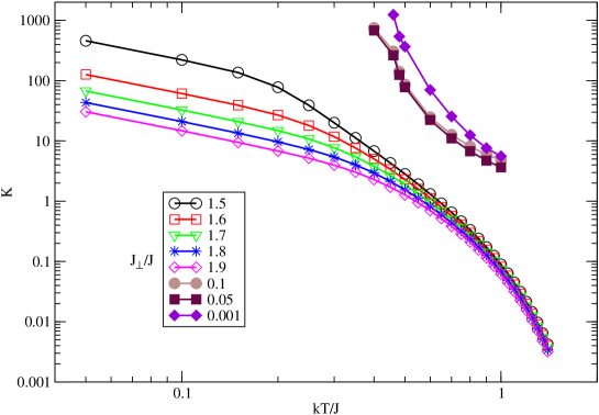
Figure 1: Thermal conductivity along leg direction versus $kT/J$ for different values of $J_{\bot}/J$ in the isotropic spin ladder ($\Delta=\delta=1$). Open symbols correspond to the strong coupling limit $J_{\bot}/J>1$ and filled symbols correspond to weak coupling $J_{\bot}/J<1$ which asymptotically reaches the ballistic chain limit by decreasing $J_{\bot}/J$ to $0.001$. A monotonic decrease versus temperature is seen for all cases.

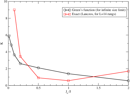
Figure 2: Thermal conductivity as a function of $J_{\bot}/J$ for $kT/J=1$, a comparison between Green’s function and exact diagonalization zotos2004 approaches in the isotropic case ($\delta=\Delta=1$). The Green’s function result represent an infinite rung ladder while the exact diagonalization one is done on 14 rungs.

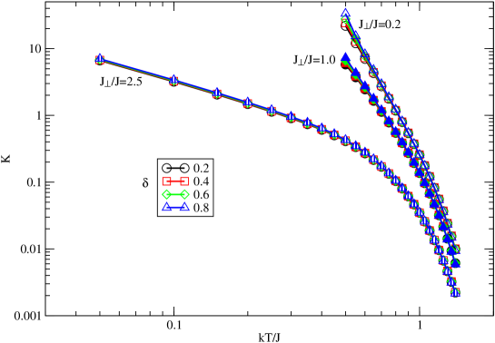
Figure 3: Variation of the thermal conductivity versus normalized temperature ($kT/J$) for different anisotropies in the leg direction ($\delta$) and for $J_{\bot}/J=0.2,1.0,2.5$, $\Delta=1$. Thermal conductivity is increased by decreasing $J_{\bot}/J$. Open symbols represent $J_{\bot}/J=0.2$, filled symbols correspond to $J_{\bot}/J=1.0$ and the striped symbols for $J_{\bot}/J=2.5$ The weak dependence on anisotropy becomes observable at low temperatures.

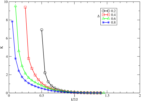
Figure 4: Thermal conductivity versus temperature ($kT/J$) for different anisotropies in the rung coupling ($\Delta$) and $J_{\bot}/J=2.5$ and $\delta=1.0$. A strong dependence on $\Delta$ is clearly observed.

References

Appendix A The explicit expression of $\mathcal{D}(k,k^{\prime},\epsilon)$

In this Appendix, we present the full expression of $\mathcal{D}(k,k^{\prime},\epsilon)$ which has been mentioned in Eq.(37). Let us first define the following relations

$$\phi_{1} = l_{2}l_{3}\Big{(}n_{B}(-l_{2}\omega_{x}(k))-n_{B}(l_{3}\omega_{z}(k+k^{\prime}))\Big{)},$$

$$\phi_{2} = l_{2}\Big{(}n_{B}(\omega_{x}(q))-n_{B}(\omega_{x}(k+k^{\prime}+q))\Big{)}\Big{(}n_{B}(-l_{2}\omega_{x}(k))-n_{B}(-\omega_{x}(k+k^{\prime}+q)+\omega_{x}(q))\Big{)},$$

$$\phi_{3} = l_{2}\Big{(}n_{B}(\omega_{z}(q))-n_{B}(\omega_{x}(k+q))\Big{)}\Big{(}n_{B}(\omega_{x}(k+q)-\omega_{z}(q))-n_{B}(l_{2}\omega_{z}(k+k^{\prime}))\Big{)},$$

$$\phi_{4} = l_{2}\Big{(}n_{B}(\omega_{x}(q))-n_{B}(\omega_{z}(k+q))\Big{)}\Big{(}n_{B}(\omega_{z}(k+q)-\omega_{x}(q))-n_{B}(l_{2}\omega_{z}(k+k^{\prime}))\Big{)},$$

$$\phi_{5} = \Big{(}n_{B}(\omega_{x}(q))-n_{B}(\omega_{x}(k+k^{\prime}+q))\Big{)}\Big{(}n_{B}(\omega_{z}(q))-n_{B}(\omega_{x}(k+q))\Big{)}$$

$$\times \Big{(}n_{B}(\omega_{x}(k+q^{\prime})-\omega_{z}(q))-n_{B}(\omega_{x}(q^{\prime})-\omega_{x}(k+k^{\prime}+q))\Big{)}$$

$$\phi_{6} = \Big{(}n_{B}(\omega_{x}(q))-n_{B}(\omega_{x}(k+k^{\prime}+q))\Big{)}\Big{(}n_{B}(\omega_{x}(q))-n_{B}(\omega_{z}(k+q))\Big{)},$$

$$\times \Big{(}n_{B}(\omega_{z}(k+q^{\prime})-\omega_{x}(q))-n_{B}(\omega_{x}(q^{\prime})-\omega_{x}(k+k^{\prime}+q))\Big{)},$$

$$\lambda_{1} = n_{B}(\omega_{z}(q_{1}))-n_{B}(\omega_{x}(k^{\prime}+q_{1})),$$

$$\lambda_{2} = n_{B}(\omega_{x}(q_{1}))-n_{B}(\omega_{z}(k^{\prime}+q_{1})).$$

Based on the above definitions, $\mathcal{D}(k,k^{\prime},\epsilon)$ is given by

$$\mathcal{D}(k,k^{\prime},\epsilon)=\mathcal{D}_{1}(k,k^{\prime},\epsilon)+\mathcal{D}_{2}(k,k^{\prime},\epsilon)+\mathcal{D}_{3}(k,k^{\prime},\epsilon)+\mathcal{D}_{4}(k,k^{\prime},\epsilon)+\mathcal{D}_{5}(k,k^{\prime},\epsilon)+\mathcal{D}_{6}(k,k^{\prime},\epsilon),$$ (39)

where

$$\mathcal{D}_{1}(k,k^{\prime},\epsilon) = -4\Big{(}\sum_{l_{1},l_{2},l_{3}=\pm}l_{1}\phi_{1}Im(1/(\epsilon-l_{1}\omega_{x}(k^{\prime})+i0^{+}))Im(1/(-\epsilon-l_{2}\omega_{x}(k)-l_{3}\omega_{z}(k+k^{\prime})-i0^{+}))$$

$$+ \frac{1}{N}\sum_{l_{1}=\pm,l_{2}=\pm,q_{1}}\lambda_{1}\phi_{1}Im(1/(\epsilon-\omega_{z}(q_{1})+\omega_{x}(k+k^{\prime}+q_{1})+i0^{+}))Im(1/(-\epsilon-l_{1}\omega_{x}(k)-l_{2}\omega_{z}(k+k^{\prime})-i0^{+}))$$

$$+ \frac{1}{N}\sum_{l_{1}=\pm,l_{2}=\pm,q_{1}}\lambda_{2}\phi_{1}Im(1/(\epsilon-\omega_{x}(q_{1})+\omega_{z}(k+k^{\prime}+q_{1})+i0^{+}))Im(1/(-\epsilon-l_{1}\omega_{x}(k)-l_{2}\omega_{z}(k+k^{\prime})-i0^{+}))\Big{)},$$

$$\mathcal{D}_{2}(k,k^{\prime},\epsilon) = -8\frac{1}{N}\Big{(}\sum_{l_{1},l_{2}=\pm,q}l_{1}\phi_{2}Im(1/(\epsilon-l_{1}\omega_{x}(k^{\prime})+i0^{+}))Im(1/(-\epsilon-l_{2}\omega_{x}(k)-\omega_{x}(q)+\omega_{x}(k+k^{\prime}+q)-i0^{+}))$$

$$+ \frac{1}{N}\sum_{l_{1}=\pm,q,q_{1}}\lambda_{1}\phi_{2}Im(1/(\epsilon-\omega_{z}(q_{1})+\omega_{x}(k^{\prime}+q_{1})+i0^{+}))Im(1/(-\epsilon-l_{1}\omega_{x}(k)-\omega_{x}(q)+\omega_{x}(k+k^{\prime}+q)-i0^{+}))$$

$$+ \frac{1}{N}\sum_{l_{1}=\pm,q,q_{1}}\lambda_{2}\phi_{2}Im(1/(\epsilon-\omega_{x}(q_{1})+\omega_{z}(k^{\prime}+q_{1})+i0^{+}))$$

$$\times Im(1/(-\epsilon-l_{1}\omega_{x}(k)-\omega_{x}(q)+\omega_{x}(k+k^{\prime}+q)-i0^{+}))\Big{)},$$

$$\mathcal{D}_{3}(k,k^{\prime},\epsilon) = -4\frac{1}{N}\Big{(}\sum_{l_{1},l_{2}=\pm,q}l_{1}\phi_{3}Im(1/(\epsilon-l_{1}\omega_{x}(k^{\prime})+i0^{+}))Im(1/(-\epsilon-l_{2}\omega_{z}(k+k^{\prime})-\omega_{z}(q)+\omega_{x}(k+q)-i0^{+}))$$

$$+ \frac{1}{N}\sum_{l_{1}=\pm,q,q_{1}}\lambda_{1}\phi_{3}Im(1/(\epsilon-\omega_{z}(q_{1})+\omega_{x}(k^{\prime}+q_{1})+i0^{+}))Im(1/(-\epsilon-l_{2}\omega_{z}(k+k^{\prime})-\omega_{z}(q)+\omega_{x}(k+q)-i0^{+}))$$

$$+ \frac{1}{N}\sum_{l_{1}=\pm,q,q_{1}}\lambda_{2}\phi_{3}Im(1/(\epsilon-\omega_{x}(q_{1})+\omega_{z}(k^{\prime}+q_{1})+i0^{+}))$$

$$\times Im(1/(-\epsilon-l_{2}\omega_{z}(k+k^{\prime})-\omega_{x}(q)+\omega_{x}(k+q)-i0^{+}))\Big{)},$$

$$\mathcal{D}_{4}(k,k^{\prime},\epsilon) = -4\frac{1}{N}\Big{(}\sum_{l_{1},l_{2}=\pm,q}l_{1}\phi_{4}Im(1/(\epsilon-l_{1}\omega_{x}(k^{\prime})+i0^{+}))Im(1/(-\epsilon-l_{2}\omega_{x}(k+k^{\prime})-\omega_{z}(q)+\omega_{z}(k+q)-i0^{+}))$$

$$+ \frac{1}{N}\sum_{l_{1}=\pm,q,q_{1}}\lambda_{1}\phi_{4}Im(1/(\epsilon-\omega_{z}(q_{1})+\omega_{x}(k^{\prime}+q_{1})+i0^{+}))Im(1/(-\epsilon-l_{2}\omega_{x}(k+k^{\prime})-\omega_{z}(q)+\omega_{z}(k+q)-i0^{+}))$$

$$+ \frac{1}{N}\sum_{l_{1}=\pm,q,q_{1}}\lambda_{2}\phi_{4}Im(1/(\epsilon-\omega_{x}(q_{1})+\omega_{z}(k^{\prime}+q_{1})+i0^{+}))$$

$$\times Im(1/(-\epsilon-l_{2}\omega_{z}(k+k^{\prime})-\omega_{x}(q)+\omega_{x}(k+q)-i0^{+}))\Big{)},$$

$$\mathcal{D}_{5}(k,k^{\prime},\epsilon) = -4\frac{1}{N}\Big{(}\sum_{l_{1}=\pm,q,q_{1}}l_{1}\phi_{5}$$

$$\times Im(1/(\epsilon-l_{1}\omega_{x}(k^{\prime})+i0^{+}))Im(1/(-\epsilon+\omega_{x}(k+k^{\prime}+q)-\omega_{z}(q^{\prime})-\omega_{z}(q)+\omega_{x}(k+q^{\prime})-i0^{+}))$$

$$+ \frac{1}{N}\sum_{l_{1}=\pm,q,q_{1},q^{\prime}}\lambda_{1}\phi_{5}Im(1/(\epsilon-\omega_{z}(q_{1})+\omega_{x}(k^{\prime}+q_{1})+i0^{+}))$$

$$\times Im(1/(-\epsilon+\omega_{x}(k+k^{\prime}+q)-\omega_{z}(q^{\prime})-\omega_{z}(q)+\omega_{x}(k+q^{\prime})-i0^{+}))$$

$$+ \frac{1}{N}\sum_{l_{1}=\pm,q,q_{1},q^{\prime}}\lambda_{2}\phi_{5}Im(1/(\epsilon-\omega_{x}(q_{1})+\omega_{z}(k^{\prime}+q_{1})+i0^{+}))$$

$$\times Im(1/(-\epsilon+\omega_{x}(k+k^{\prime}+q)-\omega_{z}(q^{\prime})-\omega_{z}(q)+\omega_{x}(k+q^{\prime})-i0^{+}))\Big{)},$$

$$\mathcal{D}_{6}(k,k^{\prime},\epsilon) = -4\frac{1}{N}\Big{(}\sum_{l_{1}=\pm,q,q_{1}}l_{1}\phi_{6}Im(1/(\epsilon-l_{1}\omega_{x}(k^{\prime})+i0^{+}))$$ (40)

$$\times Im(1/(-\epsilon+\omega_{x}(k+k^{\prime}+q)-\omega_{x}(q^{\prime})-\omega_{z}(q)+\omega_{z}(k+q^{\prime})-i0^{+}))$$

$$+ \frac{1}{N}\sum_{l_{1}=\pm,q,q_{1}}\lambda_{1}\phi_{6}Im(1/(\epsilon-\omega_{z}(q_{1})+\omega_{x}(k^{\prime}+q_{1})+i0^{+}))$$

$$\times Im(1/(-\epsilon+\omega_{x}(k+k^{\prime}+q)-\omega_{x}(q^{\prime})-\omega_{z}(q)+\omega_{z}(k+q^{\prime})-i0^{+}))$$

$$+ \frac{1}{N}\sum_{l_{1}=\pm,q,q_{1},q^{\prime}}\lambda_{2}\phi_{6}Im(1/(\epsilon-\omega_{x}(q_{1})+\omega_{z}(k^{\prime}+q_{1})+i0^{+}))$$

$$\times Im(1/(-\epsilon+\omega_{x}(k+k^{\prime}+q)-\omega_{x}(q^{\prime})-\omega_{z}(q)+\omega_{z}(k+q^{\prime})-i0^{+}))\Big{)}.$$

References

• (1) P. W. Anderson, Mater. Res. Bull 8, 2 (1973)
• (2) P. W. Anderson, Science 235 1196 (1973)
• (3) E. Dagotto, J. Riera, D. J. Scalapino, Phys. Rev. B45, 5744 (1992)
• (4) C. Hess, C. Baumann, U. Ammerahl, B. Buchner, F. Heidrich-Meissner, W. Brenig and A. Revcolevschi, Phys. Rev. B64, 184305 (2001)
• (5) A. V. Sologubenko, K. Gianno, H. R. Ott, U. Ammerahl, A. Revcolevschi, Phys. Rev. Lett 84, 2714(2000)
• (6) C. Hess, Eur. Phys. J. Special Topics, 151, 73 (2007).
• (7) X. Zotos, F. Naef, P. Prelovsek, Phys. Rev. B 55, 11029 (1997)
• (8) F. Heidrich-Meisner, A. Honecker, D. C. Cabra and W. Brenig, Phys. Rev. B 66, 140406(R) (2002)
• (9) F. Heidrich-Meisner, A. Honecker, D. C. Cabra and W. Brenig, Phys. Rev. B 68, 134436 (2003)
• (10) E. Orignac, R. Chitra and R. Citro, Phys. Rev. B 67, 134426 (2003)
• (11) K. Saito, S. Miyashita, J. Phys. Soc. Jpn 71, 2485 (2002)
• (12) N. Hlubek, et al, J. Stat. Mech. P03006 (2012)
• (13) K. Louis, P. Prelovsek and X. Zotos, Phys. Rev. B 74, 235118 (2006)
• (14) E. Shimshoni, N. Andrei and A. Rosch, Phys. Rev. B 68, 104401 (2003)
• (15) A.V. Rozhkov and A.L. Chernyshev, Phys. Rev. Lett. 94, 087201 (2005)
• (16) P. Jung, R. W. Helmes and A. Rosch, Phys. Rev. Lett, 96 067202 (2006)
• (17) M. Montagnese, M. Otter, X. Zotos,D.A. Fishman, N. Hlubek, O. Mityashkin, C. Hess, R. Saint-Martin, S. Singh, A. Revcolevschi, P. H. M. van Loosdrecht, Phys. Rev. Lett. 110, 147206 (2013)
• (18) C. Hess, P. Riberio, B. Büchner, H. ElHaes, G. Roeth, U. Ammerahl, A. Revcolevschi, Phys. Rev. B 73, 104407 (2006)
• (19) X. Zotos, Phys. Rev. Lett. 92, 067202 (2004)
• (20) E. Boulat et. al. Phys. Rev. B 76, 214411 (2007)
• (21) M. Znidaric, Phys. Rev. Lett. 110, 070602 (2013)
• (22) A. V. Chubukov, JETP Lett. 49, 129 (1989)
• (23) S. Sachdev and R. N. Bhatt, Phys. Rev. B 41, 9332 (1990)
• (24) E. C̆ižmár, M. Ozerov, J. Wosnitza, B. Thielemann, K. W. Krämer, Ch. Rüegg, O. Piovesana, M. Klanjšek, M. Horvatić, C. Berthier, and S. A. Zvyagin, Phys. Rev. B 82, 054431 (2010)
• (25) V. Kiryukhin, Y. J. Kim, K. J. Thomas, F. C. Chou, R. W. Erwin, Q. Huang, M. A. Kastner and R. J. Birgeneau, Phys. Rev. B 63, 144418 (2001)
• (26) A. Abrikosov, L.Gorkov, and T. Dzyloshinskii, Methods of Quantum Field Theory in Statistical Physics (Dover, New York, 1975)
• (27) A. L. Fetter and J. D. Walecka, Quantum Theory of Many Particle Systems (McGraw-Hill, New York, 1971 )
• (28) H. Rezania, A. Langari and P. Thalmeier, Phys.Rev. B 77, 094438 (2008)
• (29) G. D. Mahan, Many-particle physics (Kluwer Academic/Plenum Publishers, 2000)
• (30) F. Grosso and P. Parravincini, Solid state physics (Academic Press, 2000)
• (31) Indranil Paul and Gabriel Kotliar, Phys. Rev. B 67, 115131 (2003).
• (32) H. Rezania, A. Langari and P. Thalmeier, Phys.Rev. B 77, 094438 (2009)
• (33) S. Langer, R. Darradi, F. Heidrich-Meisner and W. Brenig, Phys. Rev. B 82 , 104424 (2010)