Mass distribution and structural parameters of Small Magellanic Cloud star clusters

Abstract

In this work we estimate, for the first time, the total masses and mass function slopes of a sample of 29 young and intermediate-age SMC clusters from CCD Washington photometry. We also derive age, interstellar reddening and structural parameters for most of the studied clusters by employing a statistical method to remove the unavoidable field star contamination. Only these 29 clusters out of 68 originally analysed cluster candidates present stellar overdensities and coherent distribution in their colour-magnitude diagrams compatible with the existence of a genuine star cluster. We employed simple stellar population models to derive general equations for estimating the cluster mass based only on its age and integrated light in the $B$, $V$, $I$, $C$ and $T_{1}$ filter. These equations were tested against mass values computed from luminosity functions, showing an excellent agreement. The sample contains clusters with ages between 60 Myr and 3 Gyr and masses between 300 and 3000 M_⊙ distributed between $\sim$0.5$\degr$ and $\sim$2$\degr$ from the SMC optical centre. We determined mass function slopes for 24 clusters, of which 19 have slopes compatible with that of Kroupa’s IMF ($\alpha=2.3\pm 0.7$), considering the uncertainties. The remaining clusters – H86-188, H86-190, K47, K63 and NGC242 – showed flatter MFs. Additionally, only clusters with masses lower than $\sim$1000 M_⊙ and flatter MF were found within $\sim$0.6$\degr$ from the SMC rotational centre.

1 Introduction

Since the proximity of the Magellanic Clouds (MCs) allows us to spatially resolve their stellar populations from ground based telescopes, stellar clusters have been largely used to investigate their formation and chemical evolution, namely: the star formation history (Glatt et al., 2010), the age-metallicity relationship (Piatti, 2011b) and the age distribution of their clusters (Chiosi et al., 2006; Piatti et al., 2011), among others.

Unlike the well known cluster age gap in the Large Magellanic Cloud (LMC), the formation of stellar clusters in the Small Magellanic Cloud (SMC) seems to have occurred continuously over the last 10.5 Gyr, with some periods of enhancement possibly due to the close gravitational interaction with either the Milky Way (MW) or the LMC (Glatt et al., 2008). Particularly, young and intermediate-age stellar clusters provide important information of the recent ($<$ 1 Gyr) interactions of the LMC-SMC-MW system. Investigations in this context have shown that the location of the young stellar populations of the SMC are biased towards the East side of the galaxy, while the bulk of the old population ($\sim$10 Gyr) presents a much more spherical and smooth distribution (Gardiner & Hatzidimitriou, 1992; Zaritsky et al., 2000). This trend is best noticed for stellar associations, HII regions and stellar clusters (Bica & Schmitt, 1995).

As far as we are aware, Bica et al. (2008, hereafter B08) presented the most complete compilation of extended objects in the MCs, containing over 7000 clusters and associations. However, the characterisation of such a large number of targets is beyond the scope of any single work. Therefore, many objects from that catalogue still lack their fundamental parameters while others do not correspond to physical systems at all (Piatti & Bica, 2012). Particularly, the sparse, poorly populated clusters near the central regions of these galaxies have been neglected due to the difficulties imposed by the large field contamination and source crowding.

Previous photometric studies of SMC clusters include the works of Pietrzynski & Udalski (1999), Chiosi et al. (2006), Glatt et al. (2010), Piatti (2011a) and Piatti & Bica (2012) that used colour-magnitude diagrams (CMDs) and isochrone fittings to age-date stellar clusters. Hubble Space Telescope ($HST$) data have also been used to derive the age of a few SMC clusters via CMDs (e.g. Mighell et al., 1998; Rich et al., 2000; Rochau et al., 2007; Chiosi & Vallenari, 2007).

As important as the age estimate for large samples of SMC clusters, the knowledge of their formation and evolution would benefit greatly from studies on their mass and initial mass function (IMF), despite all difficulties inherent to their derivation. Mass and IMF, combined with age information, are fundamental properties which allow a connection between dynamics and stellar evolution within a cluster. Diagnostics of mass segregation, evaporation and cluster evolutionary state become feasible if these properties are known.

Kontizas et al. (1982) have performed star counts on photographic plates obtained for 20 SMC clusters to derive their structural parameters (core and tidal radius) from King (1962) profile fittings. They estimated the cluster masses ($M_{\mathrm{clu}}$) using the King (1962) approximation for the cluster tidal radius:

$$R_{t}=d[M_{\mathrm{clu}}/(3.5M_{\mathrm{smc}})]^{1/3},$$ (1)

where $M_{\mathrm{smc}}$ is the SMC mass (3$\times$10⁹ M_⊙; de Vaucouleurs & Freeman, 1972) and $d$ is the distance between the cluster and the SMC dynamical centre, adopted as the rotation centre at RA$(1950.0)=1^{\mathrm{h}}03^{\mathrm{m}}$ and Dec.$(1950.0)=-72\degr 45\arcmin$ (Hindman, 1967; Westerlund, 1997). The above expression gave an upper mass limit because the distances used were the projected ones.

An often pursued approach, suitable to deal with large cluster samples, is to estimate masses from absolute magnitude and evolutionary models. In this context, Hunter et al. (2003) compared $UBVR$ integrated colours of 939 SMC clusters with evolutionary models to obtain their ages and masses. They further investigated the effects of fading and size-of-sample effects in star cluster analysis. Dias et al. (2010) has derived the ages and metallicities of 14 SMC clusters, using integrated spectra fitted to theoretical models. They showed that these parameters are not critically affected neither by the SSP model used nor by the fitting technique employed. Mackey & Gilmore (2003) compiled ages from the literature and determined masses for 10 populous SMC clusters from their surface brightness profiles measured from $HST$ images. Carvalho et al. (2008) fitted Elson et al. (1987) models to surface brightness profiles of 23 SMC clusters and calculated their masses, total cluster luminosities and the mass-to-light ratios as in Mackey & Gilmore (2003).

On a more direct approach a cluster luminosity function (LF) can be converted into a mass distribution by using an isochrone mass-luminosity relation. It has the advantage that, in addition to the total mass, mass function (MF) slopes can also be derived. In this context $HST$ data has been largely used to the investigation of SMC clusters, mostly due to its photometric depth and spatial resolution. Glatt et al. (2011) estimated the present-day mass function (PDMF) and the total masses of 6 clusters older than 1 Gyr, detecting the occurrence of mass segregation. Rochau et al. (2007) derived a PDMF similar to the Salpeter (1955) IMF for BS90, a 4.5 Gyr old cluster, also detecting mass segregation as a result of the cluster dynamical evolution since its age is larger than its relaxation time.

Chiosi & Vallenari (2007) estimated the IMF of the younger clusters NGC265, K29 and NGC290 (age $\sim$ 100 Myr), founding that it is compatible with that of Kroupa (2001) for masses between 0.7 and 4 M_⊙. Additional young, well-studied clusters are NGC330 (Sirianni et al., 2002; Gouliermis et al., 2004), NGC346 (Massey et al., 1995; Sabbi et al., 2008) and NGC602 (Schmalzl et al., 2008; Cignoni et al., 2009); all presenting MF slopes consistent with the Salpeter value. Mass segregation was also detected for these clusters, and suggested to be primordial as their age is smaller than their relaxation times.

We aim at increasing the number of clusters with estimated mass in the SMC, thus helping to better understand the cluster dynamical evolution in this galaxy. We made use of a recently developed method (Maia et al., 2010) to account for the field star contamination by sampling the field population from a neighbouring region and statistically removing it from the cluster CMD. Then, we estimated for the first time the total mass and mass function slopes for a sample of 29 SMC clusters. This information can be used to infer the evolutionary state of these targets and also provide additional constraints on the environmental conditions of the clusters evolution in the galaxy. For this purpose we made use of deep Washington photometry acquired at the CTIO 4m Blanco telescope, drawn from the NOAO Science Data Management Archives.

In Sect. 2 we describe the collected data, their reduction and the initial cluster sample. Sect. 3 deals with the methods used to select the cluster sample analysed in this work. Sect. 4 describes the field decontamination method and isochrone fitting. Mass functions of our targets are derived in Sect 5, where cluster mass is also estimated. In Sect 6 we discuss our results and in Sect. 7 we draw our concluding remarks.

2 Data handling and cluster selection

The photometric data used in this work were taken from the NOAO Science Data Management Archives and included several star clusters inside 11 fields distributed throughout the SMC. The images were obtained in December, 2008 at the CTIO 4m Blanco telescope with the Mosaic II camera attached ($36\times 36$ arcmin² field with a 0.27 arcsec.pixel^-1 plate scale) and the $C$ and $T_{1}$ Washington photometric filters. Exposure times in these filters were 1500s and 300s, respectively.

The reduction and the calibration of the frames were carried out using standard iraf routines from the mosaic data reduction package (mscred) and the photometry was performed using the star finding and point spread functions fitting routines from the daphot/allstar packages. The average seeing values measured in the images were 1.2″and 1.0″, in the $C$ and $T_{1}$ filters respectively. The 50% completeness level were reached at $C\sim 23-24.5$ and $T_{1}\sim 22.5-24.0$, depending on the crowding of the field, corresponding to a mass limit of $\sim 1.2\,\mathrm{M}_{\odot}$ if reddening is neglected. Further details of the data processing and of the photometry of the images are described in Piatti (2011a, 2012).

The images contained a total of 152 clusters from the B08 catalogue. Recent works on this target list have already reported 20 intermediate-age or old clusters (Piatti, 2011a, b), 4 moderately young clusters and 17 possible asterisms (Piatti & Bica, 2012). The present work focuses on a subset of the remaining sample of 68 candidate clusters, which includes potentially younger objects and asterisms.

3 Star count analysis

3.1 Density maps

A stellar density enhancement over the surrounding field is the most basic condition to identify a star cluster. However, discerning such an enhancement from field density fluctuations can be difficult, specially in dense regions.

To address this issue we constructed stellar density maps for each target in our sample. Each map was constructed by: (i) selecting stars brighter/fainter than a magnitude threshold value (see below) inside a $2\times 2$ arcmin box around the target literature coordinates; (ii) calculating the stellar density value on a circular region of 5 arcsec radius around each star; (iii) interpolating these stellar density values to a uniform grid with a resolution of $\approx 5$ arcsec and; (iv) plotting these values as a contour map.

In a tentative to probe the cluster stars distribution, we constructed a map considering only stars brighter than a magnitude threshold in the $T_{1}$ band. This threshold was defined so as to include the brightest 10 per cent of the total number of selected stars. In addition, a complementary map was also created using the stars fainter than the defined threshold to probe the field population. These maps are hereafter referred as the ”blue” and ”red” stellar density maps, respectively. Finally, additional ”blue” and ”red” density maps were also created by shifting this magnitude threshold towards fainter magnitudes at increments of 0.5 mag in order to find the magnitude limit that gives the best contrast between the cluster and field population. Five ”blue” and ”red” maps were built for each cluster candidate, following the above procedure. Fig. 1 shows the resulting density maps for the cluster H86-76.

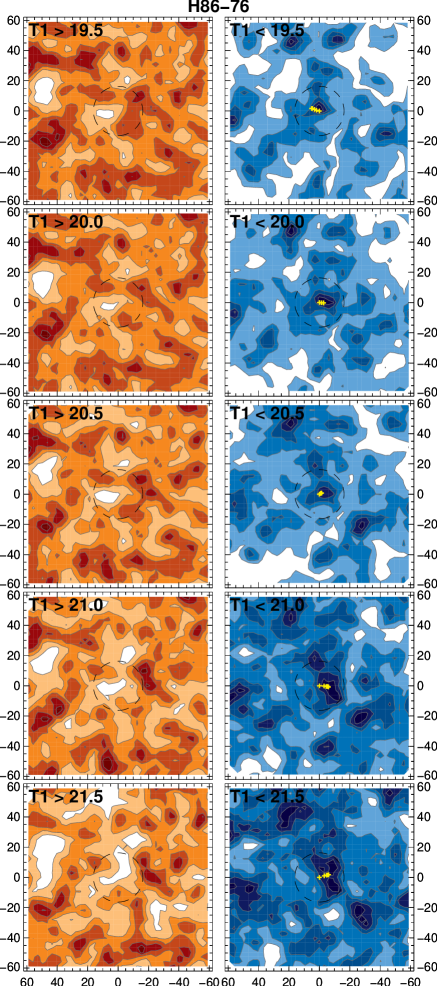
Figure 1: ”Red” (left) and ”blue” (right) stellar density maps for the cluster H86-76. In each map, darker colours represent relatively higher stelar density levels. The density levels between the maps are not related. The magnitude threshold for the top panel maps ($T_{1}=19.5$) ensures that this ”blue” map contains at least 10 per cent of the total stellar population. The dashed line represents the cluster visual radius and the yellow symbols indicate iterations of the centre finding algorithm.

It can be seen that as the magnitude threshold is increased from its initial value, the cluster becomes better defined in the ”blue” map up to a magnitude limit ($T_{1}\approx 20.5$), where the field population starts to dominate. This magnitude limit varies among our target sample, as it depends on both the cluster age and the relative stellar overdensity over the nearby field. It can be more objectively defined by using the target cumulative luminosity function (see section 4.1).

3.2 Centre calculation

The next step in characterising any cluster candidate consists in determining its centre coordinates. For this purpose, we devised an algorithm to iteratively search for a stellar density peak by calculating the density weighted average position of the stars. Given a cluster visual radius and an initial centre coordinates (B08), the algorithm: (i) selects the stars inside the cluster radius around the initial centre; (ii) calculates new centre coordinates as the mean of the selected stars position weighted by the calculated stellar density around each star; (iii) checks for convergence; (iv) either starts a new iteration by replacing the initial coordinates by the calculated coordinates or stops adopting the last calculated coordinates as the final centre coordinates.

The algorithm converges if the distance between the initial centre and the last derived centre is less than 0.5” and the stellar density at the latter is 1-$\sigma$ above the sky density fluctuations. The algorithm aborts if the maximum number of 5 iterations is reached.

This centre finding algorithm was applied to the five blue density maps of each candidate cluster. Even though any young cluster would certainly appear prominent in the ”blue” maps, the fainter stellar population of the cluster should also allow an overdensity to be detectable as the maps start sampling fainter stars. Therefore, genuine clusters should show a density enhancement in ”blue” density maps.

To be classified as a possible cluster, the centre finding algorithm must have converged on at least 3 of the 5 ”blue” maps of the candidate. Only 37 of our 68 objects met this criterion, most of them converging on all 5 density maps. Therefore, we concentrated our subsequent analysis on this selected sample of 37 cluster candidates. Fig. 1 shows the results of the centre finding algorithm applied to the ”blue” maps of the cluster H86-76 (yellow crosses).

The possible clusters selected had their centre coordinates calculated as the mean of the coordinates found in each density map. Clusters that have survived all our selection criteria (see below) have their centre coordinates (RA, Dec.) shown in Table 5.2.

3.3 Radial density profile

In order to better trace the structure and the extension of the selected targets, we constructed radial density profiles (RDPs) around their newly determined centre coordinates and compared them with the mean stellar density of the surrounding field. Candidate clusters should present an stellar overdensity over the field. Moreover, a cluster limiting radius should be clearly defined as the radius where its local stellar density intersects that of the surrounding field.

Since the clusters structure is more easily discernable from the field when its brighter stellar population are considered (see Fig. 1), we have conducted the RDP analysis by considering only stars brighter than the cluster limiting magnitude (see Sect. 4.1). Each RDP was built by calculating the stellar density inside consecutive annular bins of various sizes around the target centre coordinates, up to a radius of $\approx 100$ arcsec. The radius of the circle drawn in the blue density maps was adopted as what we called limiting radius and the mean stellar density of the surrounding field was calculated in an annulus immediately outside this limiting radius, with the same area like the internal region.

Because some targets are located at the borders of the images, or very close to another catalogued object, or on highly variable fields, the mean stellar densities of their surrounding field were calculated in an adjacent region with the same area located to the North, to the East, to the South or to the West directions of the targets, as appropriate. Fig 2 shows a schematic finding chart and the magnitude limited RDP of the cluster H86-76. The cluster limiting radius and the field sample adopted are indicated in the diagrams.

Based on the analysis of their RDPs, 4 additional targets were removed from our candidate cluster list. These underpopulous targets could not be distinguished from the surrounding field density fluctuations. Table 5.2 lists the derived limiting radii (R_l) and the mean stellar densities of the surrounding fields ($\sigma_{\mathrm{bg}}$) for the surviving clusters.

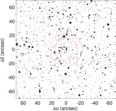
Figure 2: Schematic sky chart (left) and magnitude limited RDP (right) of the cluster H86-76. The defined limiting radius and field sampling area are indicated in the chart by the dashed and dotted lines, respectively. The cluster limiting radius and the 1-$\sigma$ interval of the field star density are represented in the RDP by the dashed and dotted lines, respectively.

In addition to the limiting radius, the central density and the core radius of the candidate clusters were also determined by fitting a 2-parameter King (1962) function to their magnitude limited radial profiles, according to the expression:

$$\sigma(r)=\sigma_{bg}+\frac{\sigma_{0}}{1+(r/R_{\mathrm{c}})^{2}},$$ (2)

where $\sigma_{bg}$ represents the background density, $\sigma_{0}$ is the central density and $R_{\mathrm{c}}$ is the core radius.

The determined $\sigma_{0}$ and R_c of the targets are shown in Table 5.2. Fig 3 shows the magnitude limited RDP of the cluster H86-76 and the fit for the determination of its structural parameters.

Moreover, a visual inspection in the derived density maps leads to conclude that 10 clusters exhibit some sign of star field substructure. In order to avoid the bulk of the field population, only the ”blue” maps presenting stars brighter than the derived magnitude limit were considered in this inspection. These 10 mostly young clusters resulted in a wide range of stellar background density, limiting radius and masses. Nevertheless, one intermediate-age cluster (BS75) and another of an interacting pair (NGC241) also present this feature.

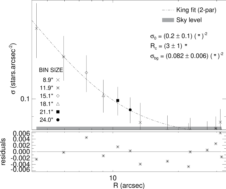
Figure 3: King profile fitted to the RDP of the cluster H86-76 (top), considering only stars brighter than its magnitude limit ($\mathrm{T}_{1}<20.8$). The fitted function (dot-slashed line), the derived structural parameters and the level of the density fluctuations of the sky (grey bar) are shown. The Poisson uncertainties and the residuals of the fit, in the sense (data - model) are also indicated for each annular bin (bottom).

4 CMD analysis

4.1 Magnitude limit

The stellar density maps employed in the determination of the centres of our targets have shown the existence of a magnitude limit for which the cluster population has an enhanced density contrast over the field. In order to better define this value, cumulative luminosity functions (CLFs) of our candidate clusters were built and compared to the CLFs of their surrounding fields.

At any given magnitude, the difference between the cluster region CLF and the surrounding field CLF should increase when the cluster population is larger than that of the field, stall when the cluster population is comparable to that of the field or decrease when the field population is larger than that of the cluster. The magnitude limit was thus given by the bin where the difference of the CLFs stalls or reach a peak. Care was taken to exclude peaks at bright magnitudes corresponding to the cluster turn-off.

Fig. 4 shows the difference between the CLF of the cluster region and the CLF of its surrounding field, built by counting stars within 0.5 magnitude bins starting from the brightest measured magnitude. The magnitude limit (M_lim) found for each target is listed in Table 5.2. A stellar density map constructed considering only stars brighter than the defined magnitude limit is also shown. The limiting radius and the field sampling area are indicated in this map.

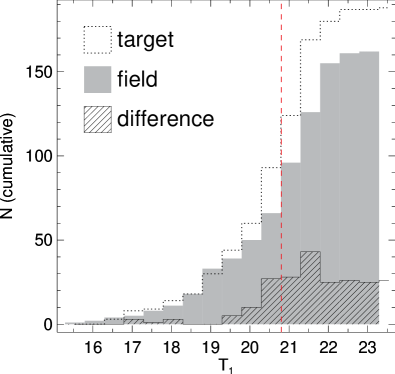
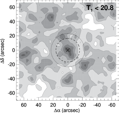
Figure 4: Difference between the cumulative luminosity functions of H86-76 region and its surrounding field (left). The defined magnitude limit is indicated by the vertical dashed line. The stellar density map considering only stars brighter than this limit (right) allows for the identification of the cluster. Its limiting radius and field sampling area are indicated by the dashed and dotted lines, respectively.

4.2 Isochrone fitting

Because of the SMC field population is dominated by a mixture of stellar populations, the CMD analysis of its clusters can be severely biased by the presence of field stars. Even when young clusters are considered, the field contamination hampers the identification of the late evolutionary sequences as their sparse bright populations are often entangled with field giant stars.

In order to mitigate this effect, a decontamination procedure was used to statistically remove the field population from the cluster CMD (Maia et al., 2010). It works by (i) sampling the field photometric characteristics in a nearby region (see Sect. 3.3); (ii) comparing with the cluster region containing members and field stars in the CMD; (iii) removing field stars from this region based on their local photometric similarity with the nearby field and on their distances from the cluster centre; (iv) assigning a photometric cluster membership value based on the local overdensity of stars in the CMD space. Previous validation tests of this method against proper motion selected members has shown that stars with membership probabilities larger than 0.3 comprises the best member sample.

Ages and colour excesses of the surviving 33 targets were then determined by means of isochrone fits to the $T_{1}\times(C$-$T_{1})$ decontaminated CMDs, giving higher priority to the most probable members (with higher assigned membership). The Padova isochrones (Marigo et al., 2008) with Z=0.004 metallicity were used. Other metallicity values were also tested (Z=0.008 and Z=0.002) but discarded since they provided a poorer fit, particularly for stars at the turn-off and at the subgiant branch regions.

Analysis of the decontaminated CMDs of our candidate clusters led us to further exclude 4 additional targets as they do not show resemblance of any evolutionary sequence on the CMD. All the 39 rejected clusters candidates are gathered in Table A (see Appendix A), with their coordinates and a remark about the criterion by which they were rejected. The 29 targets that passed through this last criterion compose our final list of studied clusters. Their derived ages and colour excesses are shown in Table 5.2. Uncertainties of these parameters were estimated by increasing/decreasing their values until a reasonable fit is no longer possible for the probable members. On average, errors from the isochrone fittings amount to $\Delta\log t\approx 0.05$ and $\Delta$E(B-V)$\approx 0.05$.

Fig. 5 compares the CMDs of the target region and of the surrounding field with the one from the decontaminated sample for the cluster H86-76. The best isochrone fitted and the limiting magnitude derived in Sect. 4.1 are also shown. For the majority of our targets the limiting magnitude derived showed good agreement with the faintest member stars left in the decontaminated CMDs.

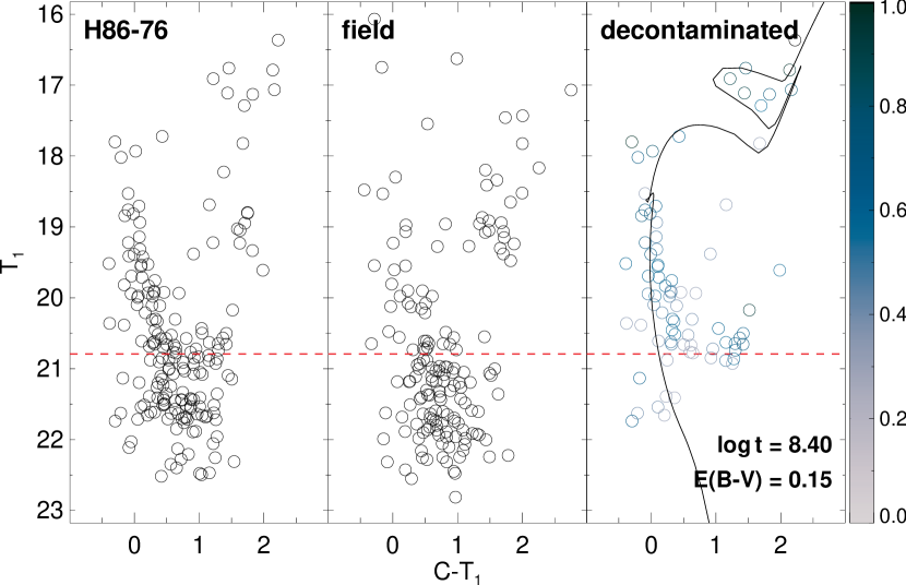
Figure 5: Extracted (left), surrounding field (middle) and decontaminated (right) CMDs of H86-76. The best fitted isochrone and its derived parameters are shown in the right panel. The coloured-bar represents the assigned membership values. The limiting magnitude is represented by the dashed line.

5 Mass distribution

The distribution of mass in a stellar cluster can yield important information on its evolutionary state and on the external environment in which it is inserted. As none of the studied clusters show any sign of their pre-natal dust or gas, their stellar components are the only source of their gravitational potential. Thus, the number of member stars and their concentration will determine, in addition to the galaxy potential, for how long clusters survive.

Since the majority of the studied clusters have ages between 100-500 Myr, mass loss due to stellar evaporation and tidal stripping play an important role in their structural evolution, which in turn may leave signs in their stellar mass distributions. In principle, an unperturbed mass distribution should resemble the cluster IMF, whereas deviances from it can be interpreted as an effect of the tidal field and of the cluster internal dynamical evolution.

To derive the mass functions of the cluster sample, luminosity functions were built by counting stars inside 0.5 mag bins along the $T_{1}$ magnitude range. In order to account for the masses of member stars, two methods have been employed to discard field stars. The first method -hereafter called CMD method- consists in constructing the LF directly from the derived decontaminated CMD (Sect. 4.2). In the second method -hereafter referred as LF method- the LF is constructed using all measured stars inside the cluster limiting radius and then subtracted from a similar LF of the surrounding field region.

To ensure homogeneity, only stars brighter than the derived magnitude limit were considered in both methods. Moreover, some clusters had their magnitude limits shifted a bin towards brighter magnitudes in order to avoid scarcely populated regions or clear field leftover in the decontaminated CMDs.

The mass distribution of each cluster was derived by using the mass-luminosity relationship obtained from the isochrone corresponding to the cluster age. Fig. 6 shows the LF and the derived MF for H86-76 using its decontaminated sample (CMD method). Fig. 7 shows the LF and MF derived for H86-76, using the difference between the cluster and surrounding field LFs (LF method).

Figure 6: Derived LF (top) and MF (bottom) of H86-76 using the CMD method for field removal. The turn-off magnitude and the corresponding mass are indicated by the dot-dashed vertical lines. The mass function fit over the main sequence stars is indicated by the solid line and by the power law exponent. The error bars correspond to the Poisson uncertainties.

Figure 7: Same as Fig 6, except that the field removed LF was built from the difference between cluster and surrounding field LFs (LF method).

It can be seen that the LF built using the LF method presents some gaps, while the one built from the CMD method shows a smoother increase of the number of stars towards fainter magnitudes. This general trend can be understood by noting that the difference between cluster and field LFs only takes into account the $T_{1}$ magnitudes of the stars, while the decontaminated sample (from which the CMD method comes from) also uses the $C$-$T_{1}$ colours and positions of the stars to better differentiate cluster and field populations.

5.1 Mass function slope

To quantify the distribution of stellar masses in a given cluster two physical parameters are of particular interest: the total mass of the cluster and the MF slope. By comparing the observed MF slope with the Kroupa (2001, hereafter K01)’s IMF slope within the corresponding mass range, one can draw information about the dynamical evolution of the cluster and diagnose processes such as mass segregation and mass loss.

The MF slope can be determined by fitting a power law function over the cluster mass distribution. Following the commonly used notation, we fitted an analytic mass function given by the power law: $\xi(m)=Am^{-\alpha}$, where $\xi(m)$ represents the mass distribution function, $\alpha$ is the power law exponent and $A$ is a normalisation constant. The power fit only considered masses smaller than the turn-off mass of the cluster. Moreover, it was only performed if 3 or more mass bins met that condition.

Although the mass distributions derived from the two methods are similar, the power law function fitted through LFs obtained from the CMD method presented, on average, lower uncertainties than those derived from the LF method. Nevertheless, whenever these two fits converged, we adopted the weighted mean of the derived exponents as the final slope of the MF and calculated its uncertainty by properly propagating the error derived from each fit.

Figs. 6 and 7 show the resulting fits of the power law and the corresponding exponent over the two mass distributions derived for H86-76. Table 5.2 lists the mean values and uncertainties of the exponent and the mass range of the power law fits for clusters for which these fits converged.

5.2 Total mass

The total mass of a cluster was calculated by initially summing up its observable mass, i.e., the sum of the masses along the different bins of its mass distribution function, including those brighter than the cluster turn-off. Secondly, the values of the mass distribution function in the lower mass regime and the MF slope given by K01 for such a mass interval were used to define the normalisation constant $A$, from which we extrapolated the power law function down to lower masses. The mass contained in these low mass ranges was estimated by integrating the extrapolated power law from the smallest observed mass bin to 0.1 solar mass. The total mass of a cluster was then estimated by adding the values obtained in these two steps. Its uncertainty was derived by propagating the errors at the individual mass bins in the observed mass distribution function and the intrinsic uncertainties of the K01 exponents in the extrapolated power law.

For H86-76 the total mass turned out to be $1405\pm 585$ M_⊙ if the mass distribution function obtained from the CMD method is used, and $1002\pm 452$ M_⊙ if that from the LF method is employed. Generally, our results indicate that the masses calculated through the CMD method were systematically higher than those calculated through the LF method, up to a factor of 2. This result suggests that, in most cases, the simple subtraction of the cluster LF from that of the field tends to underestimate the actual cluster population. The more elaborated field decontamination method not only retains a larger fraction of the cluster population, but also allow for an individual estimate of the member stars. Finally, since the uncertainties in the total masses are generally higher than the difference between the two values, we adopted the average of these masses weighted by their relative errors in the subsequent analysis. Its uncertainty was derived by propagating the errors of the two individual determinations. These results are shown in Table 5.2.

Appendix C compiles the general and magnitude limited density maps, the radial density profile, the cumulative luminosity function, the decontaminated CMD, and the field-subtracted LF and MF charts used in the analysis of each cluster. They are only available in the online version of the Journal.

Table 1: Determined parameters for the studied clusters

Target	RA	Dec.	Rl	$\sigma_{\mathrm{bg}}$		$\sigma_{0}$		Rc		Mlim	log t	E(B-V)	total mass		MF slope		MF range	Rt
	(${}^{\mathrm{h}}:^{\mathrm{m}}:^{\mathrm{s}}$)	($\degr:\arcmin:\arcsec$)	( ″)	(arcsec-2)		(arcsec-2)		( ″)					(103 M⊙)				(M⊙)	( ″)
NGC241	00:43:33	-73:26:20	23	0.186$\,\pm\,$	0.027	0.10$\,\pm\,$	0.02	9.5$\,\pm\,$	1.4	19.9	8.35	0.00	2.2$\,\pm\,$	0.7	2.2$\,\pm\,$	0.8	2.60$-$3.26	38.6$\,\pm\,$	4.2
NGC242	00:43:38	-73:26:26	20	0.196$\,\pm\,$	0.028	0.08$\,\pm\,$	0.01	6.2$\,\pm\,$	0.7	20.0	7.80	0.05	1.1$\,\pm\,$	0.4	0.8$\,\pm\,$	0.2	3.01$-$6.05	31.1$\,\pm\,$	3.3
H86-76	00:46:01	-73:23:44	16	0.196$\,\pm\,$	0.016	0.23$\,\pm\,$	0.13	3.1$\,\pm\,$	1.2	20.8	8.40	0.15	1.2$\,\pm\,$	0.4	2.1$\,\pm\,$	0.7	2.23$-$3.23	28.7$\,\pm\,$	2.9
H86-85	00:46:55	-73:25:24	20	0.175$\,\pm\,$	0.019	0.16$\,\pm\,$	0.11	2.7$\,\pm\,$	1.1	19.8	7.90	0.15	1.4$\,\pm\,$	0.6	2.3$\,\pm\,$	0.2	3.51$-$5.50	29.4$\,\pm\,$	3.9
H86-87	00:47:06	-73:22:23	24	0.192$\,\pm\,$	0.012	0.04$\,\pm\,$	0.01	10.4$\,\pm\,$	1.4	19.7	8.10	0.10	3.1$\,\pm\,$	1.7	$-$		$-$	37.6$\,\pm\,$	6.7
H86-90	00:47:25	-73:27:29	16	0.176$\,\pm\,$	0.027	0.32$\,\pm\,$	0.51	2.0$\,\pm\,$	1.8	20.4	8.40	0.00	0.8$\,\pm\,$	0.3	1.9$\,\pm\,$	0.6	2.23$-$3.23	24.4$\,\pm\,$	3.4
H86-97	00:48:12	-73:26:47	23	0.155$\,\pm\,$	0.018	0.16$\,\pm\,$	0.03	5.6$\,\pm\,$	0.7	19.5	8.10	0.05	3.3$\,\pm\,$	1.3	2.4$\,\pm\,$	0.7	3.27$-$4.41	37.7$\,\pm\,$	4.8
B48	00:48:37	-73:24:56	31	0.171$\,\pm\,$	0.010	0.03$\,\pm\,$	0.00	12.9$\,\pm\,$	1.9	18.4	7.90	0.00	3.4$\,\pm\,$	1.6	$-$		$-$	37.0$\,\pm\,$	5.9
L39	00:49:18	-73:22:18	16	0.200$\,\pm\,$	0.017	0.21$\,\pm\,$	0.07	4.2$\,\pm\,$	1.3	20.0	8.05	0.05	1.5$\,\pm\,$	0.5	3.1$\,\pm\,$	0.2	2.85$-$4.61	26.9$\,\pm\,$	3.0
SOGLE196a	00:49:27	-73:23:53	16	0.123$\,\pm\,$	0.107	0.09$\,\pm\,$	0.01	7.6$\,\pm\,$	1.0	19.9	8.35	0.00	1.0$\,\pm\,$	0.3	1.4$\,\pm\,$	0.6	2.60$-$3.39	23.6$\,\pm\,$	2.6
B55	00:50:21	-73:23:14	24	0.181$\,\pm\,$	0.025	0.67$\,\pm\,$	0.73	2.2$\,\pm\,$	1.3	19.9	8.40	0.00	1.3$\,\pm\,$	0.6	1.8$\,\pm\,$	1.0	2.54$-$3.23	24.6$\,\pm\,$	3.9
BS75	00:54:31	-74:11:07	27	0.105$\,\pm\,$	0.011	0.11$\,\pm\,$	0.03	10.1$\,\pm\,$	2.3	22.4	9.25	0.00	1.2$\,\pm\,$	0.4	2.3$\,\pm\,$	0.6	1.17$-$1.43	32.4$\,\pm\,$	3.9
BS80	00:56:14	-74:09:22	27	0.092$\,\pm\,$	0.011	0.15$\,\pm\,$	0.02	7.0$\,\pm\,$	0.6	22.4	9.45	0.00	1.5$\,\pm\,$	0.4	$-$		$-$	33.4$\,\pm\,$	3.1
H86-174	00:57:18	-72:55:58	16	0.128$\,\pm\,$	0.013	0.20$\,\pm\,$	0.16	2.7$\,\pm\,$	1.3	20.4	8.65	0.00	0.6$\,\pm\,$	0.2	$-$		$-$	9.9$\,\pm\,$	1.0
HW32	00:57:20	-71:10:13	24	0.043$\,\pm\,$	0.009	0.05$\,\pm\,$	0.01	7.4$\,\pm\,$	1.4	21.9	7.90	0.00	0.3$\,\pm\,$	0.1	1.9$\,\pm\,$	0.1	1.44$-$5.24	15.4$\,\pm\,$	1.2
H86-188	01:00:14	-72:27:30	32	0.054$\,\pm\,$	0.005	0.02$\,\pm\,$	0.01	13.5$\,\pm\,$	1.3	19.9	8.10	0.00	1.0$\,\pm\,$	0.4	1.1$\,\pm\,$	0.4	2.82$-$4.21	5.5$\,\pm\,$	0.7
H86-190	01:00:33	-72:15:30	16	0.050$\,\pm\,$	0.018	0.02$\,\pm\,$	0.01	7.1$\,\pm\,$	3.2	20.4	7.70	0.00	0.4$\,\pm\,$	0.1	1.3$\,\pm\,$	0.2	2.51$-$6.93	4.5$\,\pm\,$	0.5
K43	01:00:49	-73:20:56	23	0.145$\,\pm\,$	0.014	0.08$\,\pm\,$	0.01	10.2$\,\pm\,$	2.0	20.2	8.10	0.10	2.1$\,\pm\,$	0.7	1.5$\,\pm\,$	0.2	2.82$-$4.21	19.2$\,\pm\,$	2.1
B103	01:00:56	-73:09:06	22	0.111$\,\pm\,$	0.013	0.08$\,\pm\,$	0.02	5.9$\,\pm\,$	0.8	19.7	8.40	0.10	1.3$\,\pm\,$	0.5	$-$		$-$	12.8$\,\pm\,$	1.6
B99	01:01:24	-73:14:25	24	0.108$\,\pm\,$	0.016	0.06$\,\pm\,$	0.01	6.3$\,\pm\,$	1.0	20.2	8.10	0.10	1.0$\,\pm\,$	0.3	2.5$\,\pm\,$	0.5	2.82$-$4.41	12.9$\,\pm\,$	1.5
B111	01:01:58	-71:01:13	22	0.038$\,\pm\,$	0.006	0.21$\,\pm\,$	0.13	3.5$\,\pm\,$	1.2	22.4	9.15	0.00	0.5$\,\pm\,$	0.1	2.1$\,\pm\,$	0.9	1.19$-$1.64	19.1$\,\pm\,$	1.7
K47	01:03:11	-72:16:25	22	0.050$\,\pm\,$	0.013	0.03$\,\pm\,$	0.01	10.6$\,\pm\,$	1.2	19.9	7.90	0.00	0.6$\,\pm\,$	0.3	0.9$\,\pm\,$	0.3	2.95$-$5.24	3.3$\,\pm\,$	0.5
B124	01:05:02	-73:02:34	16	0.134$\,\pm\,$	0.015	0.28$\,\pm\,$	0.17	2.5$\,\pm\,$	0.9	20.4	8.00	0.00	0.4$\,\pm\,$	0.1	2.3$\,\pm\,$	0.2	2.42$-$4.82	6.8$\,\pm\,$	0.6
HW52	01:06:57	-73:14:06	24	0.128$\,\pm\,$	0.015	0.13$\,\pm\,$	0.02	8.2$\,\pm\,$	1.0	21.5	8.10	0.05	0.8$\,\pm\,$	0.2	1.8$\,\pm\,$	0.2	1.68$-$4.41	11.8$\,\pm\,$	1.0
K55	01:07:31	-73:07:11	32	0.127$\,\pm\,$	0.014	0.25$\,\pm\,$	0.05	8.9$\,\pm\,$	1.3	21.9	8.45	0.00	1.9$\,\pm\,$	0.4	2.0$\,\pm\,$	0.1	1.41$-$2.85	13.7$\,\pm\,$	1.0
K57	01:08:14	-73:15:25	32	0.116$\,\pm\,$	0.013	0.19$\,\pm\,$	0.02	7.1$\,\pm\,$	0.5	20.9	8.65	0.00	1.9$\,\pm\,$	0.5	2.2$\,\pm\,$	0.5	1.82$-$2.48	16.7$\,\pm\,$	1.5
B134	01:09:01	-73:12:24	24	0.106$\,\pm\,$	0.011	0.05$\,\pm\,$	0.01	12.3$\,\pm\,$	1.9	20.9	8.15	0.00	0.6$\,\pm\,$	0.2	1.7$\,\pm\,$	0.2	1.99$-$4.21	11.0$\,\pm\,$	1.1
K61a	01:09:02	-73:05:11	23	0.131$\,\pm\,$	0.032	0.07$\,\pm\,$	0.01	11.1$\,\pm\,$	1.6	20.9	8.30	0.00	1.1$\,\pm\,$	0.3	2.6$\,\pm\,$	0.1	1.95$-$3.39	11.7$\,\pm\,$	1.1
K63	01:10:47	-72:47:31	32	0.099$\,\pm\,$	0.009	0.10$\,\pm\,$	0.01	13.2$\,\pm\,$	0.8	21.4	8.25	0.00	1.0$\,\pm\,$	0.2	1.3$\,\pm\,$	0.2	1.66$-$3.51	9.1$\,\pm\,$	0.7

Note: ^a structural parameters were derived by using semi-annular bins to avoid a nearby CCD gap. Likewise, the LF and MF of these targets were corrected to account for the cluster area lost in the gap.

5.2.1 SSP models

The cluster masses were also determined by using their integrated magnitudes and ages and by employing single-burst stellar population (SSP) models as built from Padova isochrones. The SSPs contain stars in the mass range $0.08<m$(M_⊙)$<120$ distributed according to a Kroupa IMF with the total mass normalised to one. SSPs were generated for ages $6.6<\log{t(yr)}<10.1$ and for metallicities $Z=0.019$, 0.008 and 0.004.

We started by first computing the evolution of the SSP mass-luminosity ratio ($\mathcal{M}/\mathcal{L}$), which does not depend on the IMF normalisation constant. Operationally, for a cluster of a given age, its $\mathcal{M}/\mathcal{L}$ is derived from the models; then, its mass is determined using the integrated absolute magnitude. Fig. 8 shows the $\mathcal{M}/\mathcal{L}$ evolution in the $T_{1}$ magnitude for SSPs with metallicities $Z=0.004$ and 0.019. The label ’Initial mass’ refers to models where the total SSP mass remains constant (equal to one) along the cluster evolution, while the label ’Isochrone mass’ refers to the total mass computed using the actual isochrone stellar masses, which naturally changes with age. For the $T_{1}$ mag, it can be seen that the difference in $\mathcal{M}/\mathcal{L}$ ratio for ages larger than 100 Myr due to the different total mass prescriptions adopted are twice as large as that produced by a metallicity variation of $\Delta Z=0.015$.

Figure 8: The $T_{1}$ magnitude evolution of the mass-luminosity ratio according to SSP models of different metallicities and different ways of computing the total mass.

The models for which the total mass was computed from the isochrones should reproduce better the evolution of real clusters because mass loss effects due to the stellar evolution are accounted for. Stellar remnants are also excluded from the total mass computed from the isochrones. However, even if a cluster retains a substantial content of stellar remnants, its mass fraction is small (see Appendix B), which makes their contribution to the total mass (and light) also small.

The $\mathcal{M}/\mathcal{L}$ ratio evolution in various filters ($BVICT_{1}$) for models including mass loss is shown in Fig. 9 for $Z=0.019$ and 0.004. The $T_{1}$ filter is very similar to the Johnson $R$ filter. It is worth noticing that the $\mathcal{M}/\mathcal{L}$ ratio has a narrow range ($\sim 0.4$ dex) around $\log{t(yr)}\sim 9$ for the various filters and metallicities. After $\log{t(yr)}=9$, the SSPs’ $\mathcal{M}/\mathcal{L}$ ratio spread, reaching $\sim 0.6$ dex at the age of $\log{t(yr)}=10$ for the extreme wavelength filters $C$ and $I$. The largest $\mathcal{M}/\mathcal{L}$ ratio difference occurs for the youngest SSPs, reaching about 1.0 dex at $\log{t(yr)}=6.7$. For ages older than 1 Gyr, the $\mathcal{M}/\mathcal{L}$ ratio in the $I$ band is less sensitive to metallicity and its evolution is smoother than that for the shorter wavelength filters. The contrary occurs for the $C$ filter.

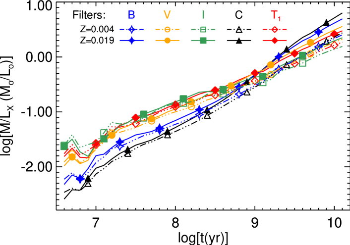
Figure 9: Multicolour evolution of the mass-luminosity ratio according to SSP models of different metallicities and including mass loss effects.

The cluster $\mathcal{M}/\mathcal{L}$ ratio is determined by interpolating its derived age in the relations shown in Fig. 9 for the filters $T_{1}$ and $C$, generated from the SSP models with $Z=0.004$ (SMC global metallicity) and taking into account mass loss effects. Cluster masses were then obtained by means of their integrated $M_{T_{1}}$ and $M_{C}$ magnitudes computed from two methods (Sect. 5): (i) by summing up the flux of the member stars as coming from the decontaminated sample (CMD method), and (ii) by integrating the cluster luminosity function after subtracting the surrounding field luminosity function (LF method).

The resulting cluster masses as a function of their ages are presented in Figs. 10 and 11. Mass uncertainties were propagated from the integrated magnitudes and ages. Because a SSP fades with time as an effect of the stellar evolution, the SSP mass at a fixed luminosity depends on the age. At any age, the SSP mass increases with its luminosity, reflecting the population size. According to these models, our cluster sample consists of systems with masses between 300 and 3000 M_⊙.

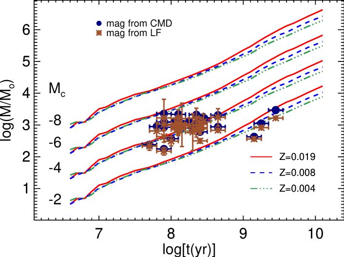
Figure 10: Distribution of masses as a function of age for the clusters in our sample. Masses were derived from the mass-luminosity ratio and the integrated $C$ magnitude according to the CMD (blue circles) and LF (brown asterisks) methods, respectively. Models of constant absolute $C$ magnitude for metallicities $Z=0.004$, $Z=0.008$, $Z=0.019$ are superimposed with dot-dashed, dashed and continuous lines, respectively.

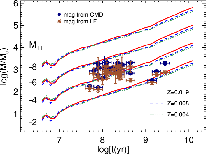
Figure 11: As in Fig. 10 but for integrated $T_{1}$ magnitude.

Figs. 10 and 11 can be also employed to estimate our photometric mass limits. For instance, from Fig. 11 it is possible to infer the photometric depth needed to reach a 1000 M_⊙ cluster in the SMC (true distance modulus ($m-M$)_∘=18.9). Thus, for a 10 Myr old cluster, its integrated $T_{1}$ magnitude should be $T_{1}=M_{T_{1}}+A_{T_{1}}+18.9\sim 12.0$, neglecting the extinction. For a 1 Gyr old cluster, the integrated mag limit results $T_{1}\sim 16.0$. Such a difference is a consequence of the clusters fading as they become older. Similarly, the cluster integrated $C-T_{1}$ colours, calculated from the CMD method, also match the respective evolution of the SSP models, as shown in Fig. 12. Note that stochastic variations in the cluster light produced by bright stars may lead to significant colour fluctuations, especially for the youngest and less populous clusters.

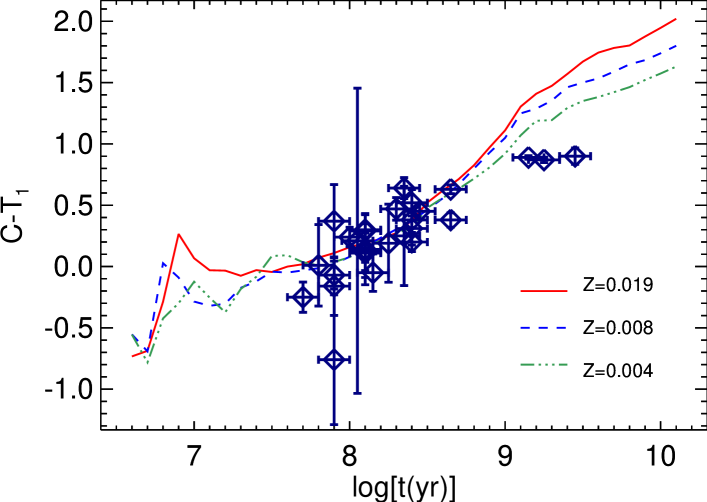
Figure 12: The colour evolution of the cluster sample is compared to that resulting from SSP models for different metallicities.

A comparison between the masses obtained from SSP models using the integrated $C$ and $T_{1}$ magnitudes and those estimated using star counts (Sect. 5.2) shows a reasonable agreement (Fig. 13). It is clear that the cluster masses derived from the CMD method (panel a) provides a better match than those obtained from the LF method (panel b), where a larger spread and a systematic deviation for lower masses is seen. In addition, the resulting masses from SSP models do not seem to depend on whether the integrated $C$ or $T_{1}$ mag is used as input. Although both mass computations make use of the same isochrone set, the significantly different approaches leading to compatible values strongly support their reliability. For this reason we derived analytic relations in order to estimate the cluster mass from the knowledge of its age and integrated magnitude. Their implementation is based on a least square fit of a straight line passing over the flat interval of the $\mathcal{M}/\mathcal{L}$ relationship for SSPs older than $\log{t(yr)}=7.3$ (20 Myr). The fits were performed for all the filters presented in Fig. 9, according to the eq. 3:

$$\log\left[{\frac{\mathcal{M}}{\mathcal{L}}}\left(\frac{{\rm M}_{\odot}}{{\rm L}_{\odot}}\right)\right]=a+b\log{[t(yr)]}\ \ \ (\log{t}>7.3)$$ (3)

The resulting correlation coefficients were superior to 0.99 in all cases. The fitted coefficients at different metallicities are summarised in Table 5.2.1.

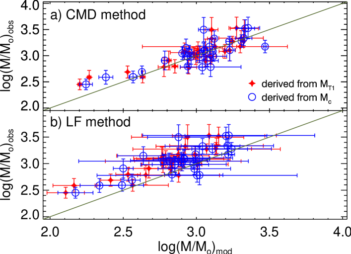
Figure 13: Comparison of cluster masses derived from star counting (’obs’) and SSP modelling (’mod’). The continuous line is the one-to-one relation.

Table 2: Linear fit coefficients for the $\mathcal{M}/\mathcal{L}$ evolution

The mass can be obtained from the integrated magnitude by rewriting eq. 3 as:

$$\log\mathcal{M}=a+b\ \log{t}-0.4(M_{n}-M_{n,\odot})$$ (4)

where $n=B,V,I,C,T_{1}$ and $M_{B,\odot}=5.49$, $M_{V,\odot}=4.83$, $M_{I,\odot}=4.13$, $M_{C,\odot}=5.68$, $M_{T_{1},\odot}=4.47$ are the Sun absolute magnitudes and $M_{n}$ the integrated absolute magnitude in the corresponding filter. Its uncertainty results in:

$$\sigma_{\log\mathcal{M}}=\sqrt{\sigma_{a}^{2}+(\log^{2}{t})\sigma_{b}^{2}+b^{2}\sigma_{\log{t}}^{2}+0.4^{2}\sigma_{M}^{2}}$$ (5)

Fig. 14 compares the masses derived by using eq. 4 and those obtained from integrated magnitudes and the interpolated $\mathcal{M}/\mathcal{L}$ ratios at the cluster ages. As can be seen, there is a tight correlation between masses coming from both procedures. We recall however, that the applicability range of these relations is limited to clusters after the embedded initial phases, i.e., older than 20 Myr. The above analysis shows that the cluster masses estimated in Sect. 5.2 are compatible with those derived from their integrated properties and from the analytic relations provided.

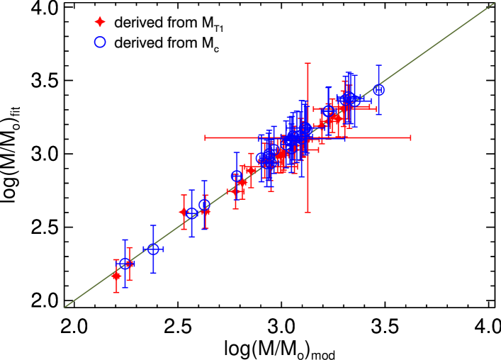
Figure 14: Comparison of cluster masses derived from interpolations (abscissa) or fits to the $\mathcal{M}/\mathcal{L}$ relations (ordinate). The continuous line is the one-to-one relation.

6 Discussion

Fig. 15 (left panel) compares our age estimates with the values obtained by Chiosi et al. (2006) and Glatt et al. (2010) for 15 and 18 clusters in common, respectively. Although we found a good agreement in the age range between $7.5<\log t<9.0$, it seems that we have overestimated the age of the young clusters K47 and H86-190. This could likely be caused by the saturation limit of our images which prevented us from identifying a turn-off brighter than T${}_{1}\sim 16$. On the other hand, previous age estimates for the two oldest clusters (BS75 and BS80) may have their published ages biased to younger values, since these clusters present a faint turn-off and the authors did not account for field star decontamination on their CMD analysis.

The comparison between the derived limiting radii (R_l) and the values from the B08 catalogue also shows a general good agreement (see Fig. 15, right panel). However, we found that some of the smaller clusters (e.g. B111, H86-190) appear to be substantially larger than previously known, while the radii of some of the largest clusters (e.g. K43) were truncated by CCD gaps in our images, leading to deceivingly smaller limiting radii.

Concerning the MF slope variation, clusters H86-188, H86-190, K47 and K63 clearly present flatter MF slopes than prescribed by K01 IMF ($\alpha=2.3\pm 0.7$). Similarly, NGC242, which does have the lowest MF slope value within the studied cluster sample ($\alpha=0.8$), forms a known interacting pair with NGC241 ($\alpha=2.2$). Its flat MF slope could be the consequence of tidal stripping by the larger, more massive cluster, NGC241. On the other hand, L39, located in a crowded field and placed close to a CCD gap, presents the steepest MF slope in the sample. In this case, the field subtraction method resulted more prone to include field leftover stars in their decontaminated sample.

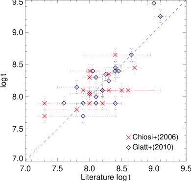
Figure 15: Correlation between derived and published ages (left) and radii (right). The dashed line corresponds to the one-to-one relation.

Although our cluster sample is not homogeneously distributed, neither spatially nor chronologically, the analysis of the derived cluster parameters can still provide important information regarding the galactic environment and its impact on the evolution of the cluster population. Fig. 16 shows the positions of the studied clusters with respect to the SMC optical centre (RA$(J2000)=00^{\mathrm{h}}52^{\mathrm{m}}45^{\mathrm{s}}$, Dec.$(J2000)=-72\degr 49\arcmin 43\arcsec$; de Vaucouleurs et al., 1976). It can be seen that the rotational centre, represented with a plus sign, is displaced from both the SMC bar (Westerlund, 1997) and the optical centre. In addition, the youngest clusters are preferentially found near the bar, while the oldest ones are located more than $\sim$ 1$\degr$ away.

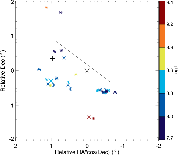
Figure 16: Cluster positions relative to the optical centre (cross). The SMC bar (line) and the rotational centre (plus) are also shown. The right-hand colourbar is scaled with the cluster age.

Fig. 17 depicts the spatial distribution of the clusters with respect to the SMC optical and rotational centres as a function of their total masses. As shown in Fig. 16, there is a segregation of the oldest clusters to the outer regions of the SMC. In addition, there seems to exist a trend of the clusters maximum mass with the distance from the SMC rotational centre.

We also analysed the cluster spatial distributions with respect to both optical and rotational SMC centres in terms of their MF slopes. The result is shown in Fig. 18. As it can be seen, clusters with any MF slope are found inside $\sim$ 1$\degr$ from the optical centre, while those located in outer regions present slopes more similar to the canonical value expected for an undisturbed population (e.g. $\alpha\sim 2.3$). Concerning the rotational centre, it seems that the clusters located inside $\sim$0.6$\degr$ present, in average, flatter MF slopes than those outside this radius.

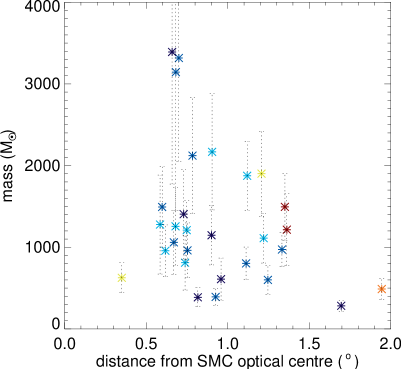
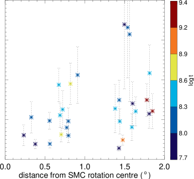
Figure 17: Cluster spatial distribution respect to the SMC optical (left) and rotational (right) centres as a function of their masses. The right-hand colourbar is as in Fig. 16.

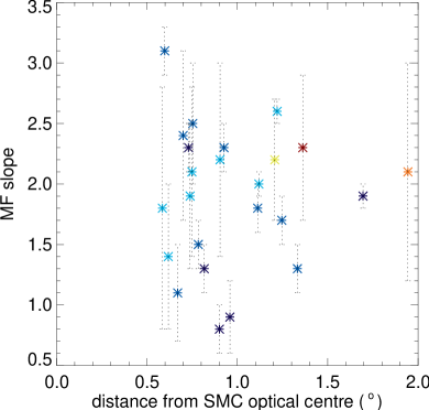
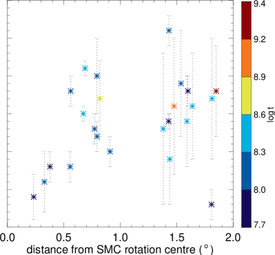
Figure 18: Cluster spatial distributions respect to the SMC optical (left) and rotational (right) centres as a function of their MF slopes. The right-hand colourbar is as in Fig. 16.

The cluster distances with respect to the rotational centre and their derived masses were also used to calculate the tidal radii through eq. 1 (see Table 5.2). As already mentioned, these values are probably underestimated, as the distances used are 2D projections of the real distances.

7 Concluding Remarks

An initial sample of 68 candidate clusters was considered for investigation. Analysis of their structures showed that 31 objects do not present a concentration of stars over the various magnitude limited density maps consistent with with the existence of a genuine star cluster. Furthermore, 4 additional objects were removed from the initial sample due to their RDPs could not be distinguished from the background fluctuations, and others 4 for showing CMD star distributions that do not correspond to cluster sequences. However, we do not rule out the possibility that some of these 39 rejected objects might still be bound systems. The 100 per cent completeness level of our photometry is reached at $T_{1}$ $\sim$ 21.5 mag. (Piatti, 2012), so that sparse clusters older than $\sim$3 Gyr could be easily overwhelmed by the field. In addition, CCD saturation caused by very bright stars contaminate the photometry of fainter stars, leaving ”holes” in the field spatial distribution of some targets. Although this effect compromised the RDP of some discarded objects, some of these targets presenting a well defined CMD were still included in the list of surviving clusters (e.g. NGC241, NGC242). Finally, since the early disruption of star clusters is a very common occurrence (Lada & Lada, 2003), it should be expected that many young objects no longer have the concentrated stellar structures found in the more populous clusters, but rather a much sparser stellar content. Such targets would certainly fail our centre finding and RDP selection methods, as their structural characteristics are akin to those of associations. Therefore, because the employed methods are not optimised to the investigation of these more challenging targets, we postpone their analysis to a forthcoming paper without placing any classification on their physical nature. These rejected candidate clusters are gathered in the Table A (Appendix A).

The remaining 29 objects compose our list of studied clusters. For these clusters we derived central coordinates, central stellar density, core, limiting and tidal radii, field stellar density, age, interstellar reddening and total mass. We also derived the MF slope for 24 clusters in our sample and found 5 clusters presenting slopes flatter than K01 IMF. Although ages and structural parameters for some of the studied clusters are available in the literature, the mass and the MF slope estimates are derived for the first time for most of them.

The cluster integrated colours and SSP mass-luminosity ratios show that the derived masses are internally consistent. Based on these results, we provide equations for computing the cluster mass using its integrated magnitude and age. These equations were derived for $B$, $V$, $I$, $C$ and $T_{1}$ magnitudes and should be useful for stellar population studies using integrated colours.

The cluster spatial distribution shows that most of the young clusters seem projected towards the SMC bar, as our cluster sample is likely to suffer from inhomogeneity and selection effects. Their maximum age, maximum mass and MF slope seem to increase with their distance from the rotational centre.

Acknowledgements

We would like to thank the anonymous referee for the valuable suggestions that helped us to improve this work. We also acknowledge the PI of the archival data used, Doug Geisler. F. F. S. Maia thanks the INCT-A and the CNPq for funding. This work was partially supported by the Argentinian institutions CONICET and Agencia Nacional de Promoción Científica y Tecnológica (ANPCyT).

Appendix A Rejected candidate clusters

Rejected clusters are gathered in Table A along with their coordinates and the criterion of rejection.

Table 3: List of rejected candidate clusters

Appendix B Contribution of stellar remnants and gas to the total mass

What are the mass contribution of stellar remnants, i.e., white dwarfs (WDs), neutron stars (NSs) and black holes (BHs) to the total mass of a star cluster of a certain age? Since the mass locked in a remnant is a fraction of the initial star mass at the Main Sequence (MS), it should be also questioned how much gas is lost or locked into the system for the subsequent star formation. Padova isochrones include both the initial mass of a star at the MS and the actual mass at an age $t$. They are different as a consequence of mass loss during the stellar evolution. Kruijssen (2009, hereafter K09) studied the evolution of the mass function in star clusters providing analytic expressions that link the star’s initial mass with the correspondent remnant mass.

To quantify the mass locked in stellar remnants and gas yielded by mass loss as predicted by Padova isochrones, we considered the relationships between the initial mass and the remnant mass given by K09 and references therein. Stars were distributed according to the Kroupa’s IMF in the mass range $0.08<m_{\circ}($M${}_{\odot})<120$ and the total mass of the SSP was normalised to 1. At a given age, stars whose initial mass ($m_{\circ}$) are higher than the initial mass of the most massive star still represented in the isochrone ($m^{iso}_{\circ}$) evolved, losing mass, to a state characterised by stellar remnants, namely WDs (if $m_{\circ}<8$ M_⊙), NSs (if 8 M${}_{\odot}\leq m_{\circ}<30$ M_⊙) and BHs (if $m_{\circ}\geq 30$M_⊙). The actual mass of the stellar remnant is then calculated using $m_{\mathrm{WD}}=0.109m_{\circ}+0.394$, $m_{\mathrm{NS}}=0.03636\,(m_{\circ}-8.)+1.02$ and $m_{\mathrm{BH}}=0.06\,(m_{\circ}-30.)+8.3$, with the SSP age defining which type of remnant is produced and the IMF giving how many remnants are formed. Notice that the younger the SSP the smaller the number of remnants and their total mass. For solar metallicity isochrones, the ages at which the different remnants have their initial mass boundaries are $t^{\ >}\!\!\!\!_{\sim}$ 40 Myr ($m^{iso}_{\circ}<8$ M_⊙) to form WDs, $6.5^{\ >}\!\!\!\!_{\sim}\ {t}^{\ >}\!\!\!\!_{\sim}$ 40 Myr ($8$ M${}_{\odot}\leq m^{iso}_{\circ}<30$ M_⊙) to form NSs, and ${t}^{\ <}\!\!\!\!_{\sim}$ 6.5 Myr ($m^{iso}_{\circ}\geq 30$ M_⊙) to form BHs, respectively. Because the actual mass in remnants is lower than their initial masses due to evolutionary mass loss, it is also possible to quantify the amount of gas released that should increase as the SSP gets older. Operationally, the difference between the total initial mass of the SSP (1 M_⊙) and the total actual mass of the stars in the isochrone plus the total actual mass in remnants gives the mass of gas yielded by the SSP.

Fig. 19 shows the mass contribution from the different components of solar metallicity SSPs as a function of their ages. The mass contribution of BHs and NSs is small regardless the SSP age, reaching at most 1.6% and 1.1%, respectively. The WDs component mass builds up after $\approx$ 40 Myr and reaches about 10% at the age of 12.6 Gyr. The gas released during the stellar evolution provides a sizeable amount of mass and dominates over the remnant contribution to the total mass as the SSP ages. It reaches about 20% and 40% of the total mass at the age of 60 Myr and 5 Gyr, respectively. In real clusters, this mass should have been transformed into stars in a secondary burst of star formation or may have been expelled from the cluster in its initial phases by stellar winds and supernova explosions. The remnant mass contribution mainly reflects the IMF combined with stellar evolution, in which WDs outnumber BHs and NSs for SSPs older than $\approx$ 500 Myr. The mass contained in an isochrone of any age is above all other contributions, but its importance decreases as the age increases.

The same analysis was done for isochrones of metallicity $Z=0.004$. The relative mass contribution as a function of age is qualitative similar to that for solar metallicity. The mass contribution of BHs and NSs are nearly identical to that for solar metallicity models, while the mass in WDs is slightly higher, reaching about 12% at the age of 12.6 Gyr. The gas mass reaches about 20% and 40% of the total mass at the age of 60 Myr and 4 Gyr, respectively.

It is worth noting that the above relative mass values are overestimates because the ignored star cluster dynamical evolution affects its original mass, especially depleting low mass stars.

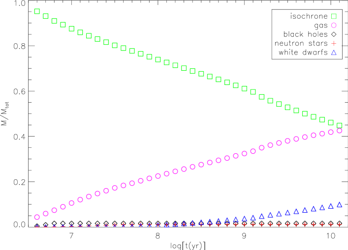
Figure 19: Mass contribution of stellar remnants and gas for SSPs of different ages.

Appendix C Selected clusters charts

All figures used in the analysis of the cluster sample are compiled in this appendix for reference. They include: magnitude limited density maps for the determination of the cluster centre, the schematic sky chart showing nearby objects and field region selected, the radial density profile for the estimation of structural parameters, the cumulative luminosity function for the estimation of the magnitude limit, the decontaminated CMD for the isochrone fitting and the field-subtracted LFs and MFs for the estimation of the mass distribution. They are only available in the online version of the Journal.

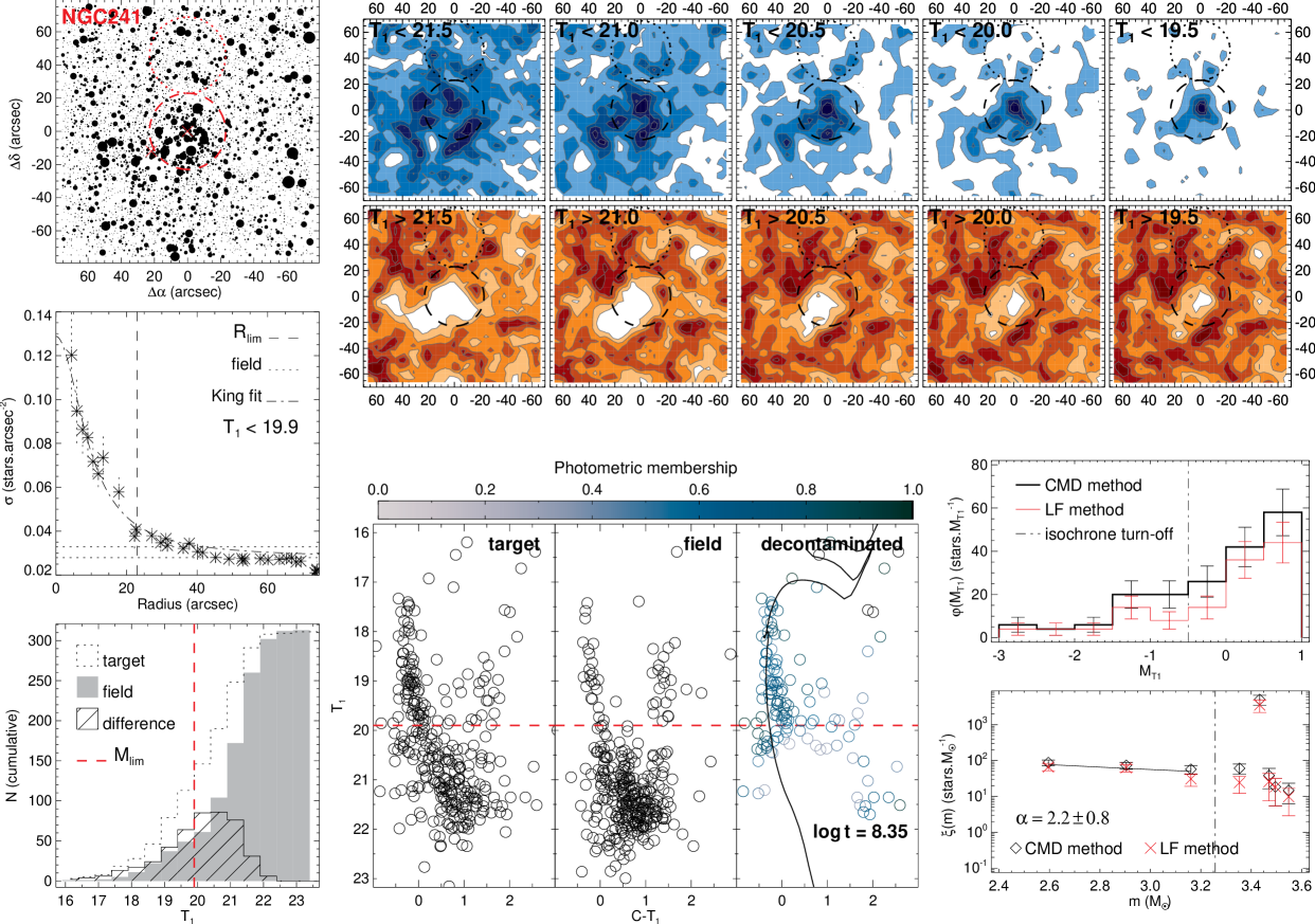
Figure 20: NGC241 analysis charts. Top-left: schematic sky chart showing the cluster (dashed line) and field (dotted line) regions adopted, along with catalogued objects (cross). Top-right: magnitude limited density maps. Middle-left: magnitude limited RDP showing the limiting radius (dashed line), the field stellar density (dotted lines) and the 2-parameter King fit (dot dashed line). Bottom-left: Cumulative LFs showing the adopted magnitude limit. Bottom-middle: CMDs comparing the cluster region, the surrounding field and the decontaminated samples; the magnitude limit derived is also shown (dashed line). Bottom-right: field-subtracted LFs and MFs according to the two methods employed; the turn-off magnitude and mass are also shown.

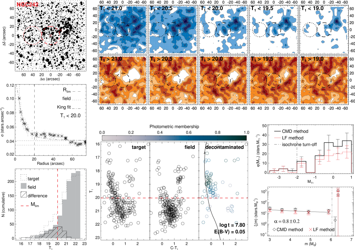
Figure 21: NGC242 analysis charts. Panels are the same as in Fig. 20

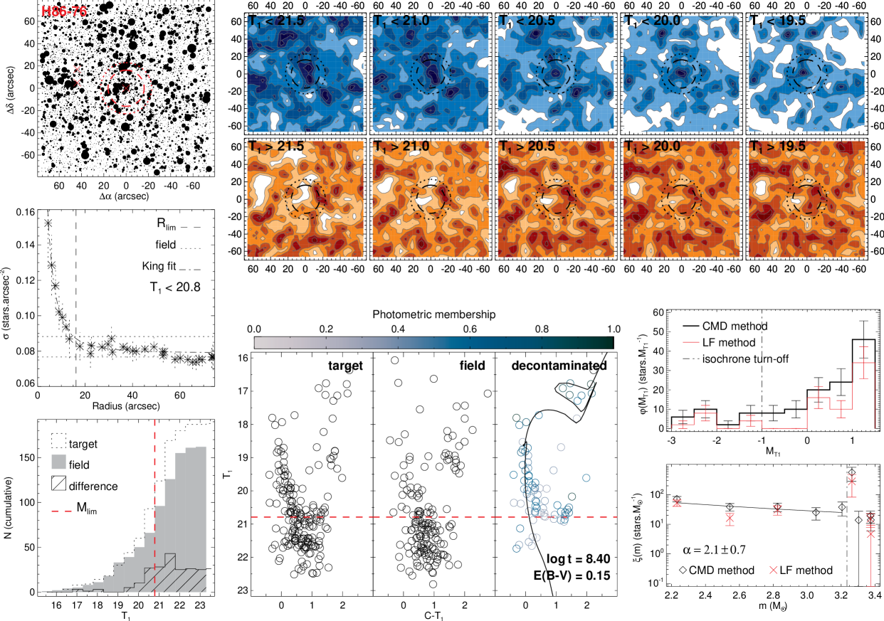
Figure 22: H86-76 analysis charts. Panels are the same as in Fig. 20

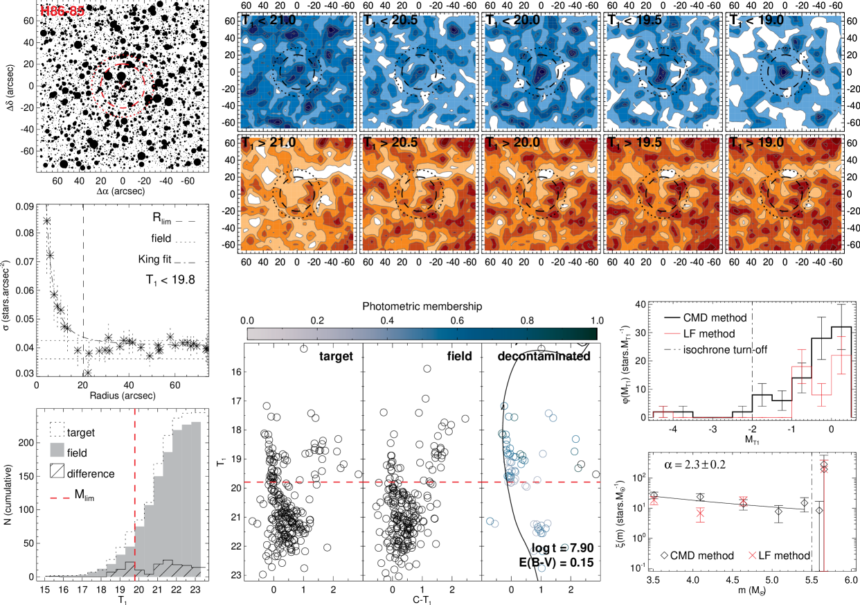
Figure 23: H86-85 analysis charts. Panels are the same as in Fig. 20

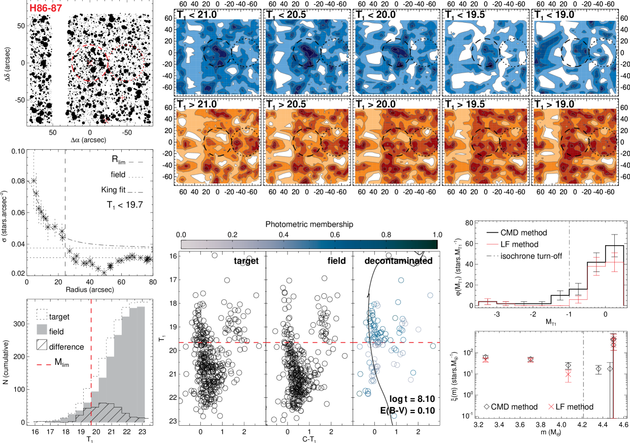
Figure 24: H86-87 analysis charts. Panels are the same as in Fig. 20

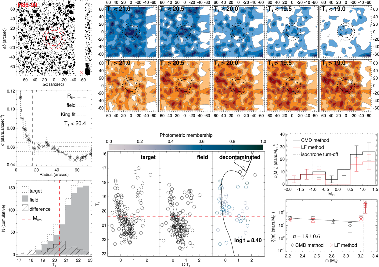
Figure 25: H86-90 analysis charts. Panels are the same as in Fig. 20

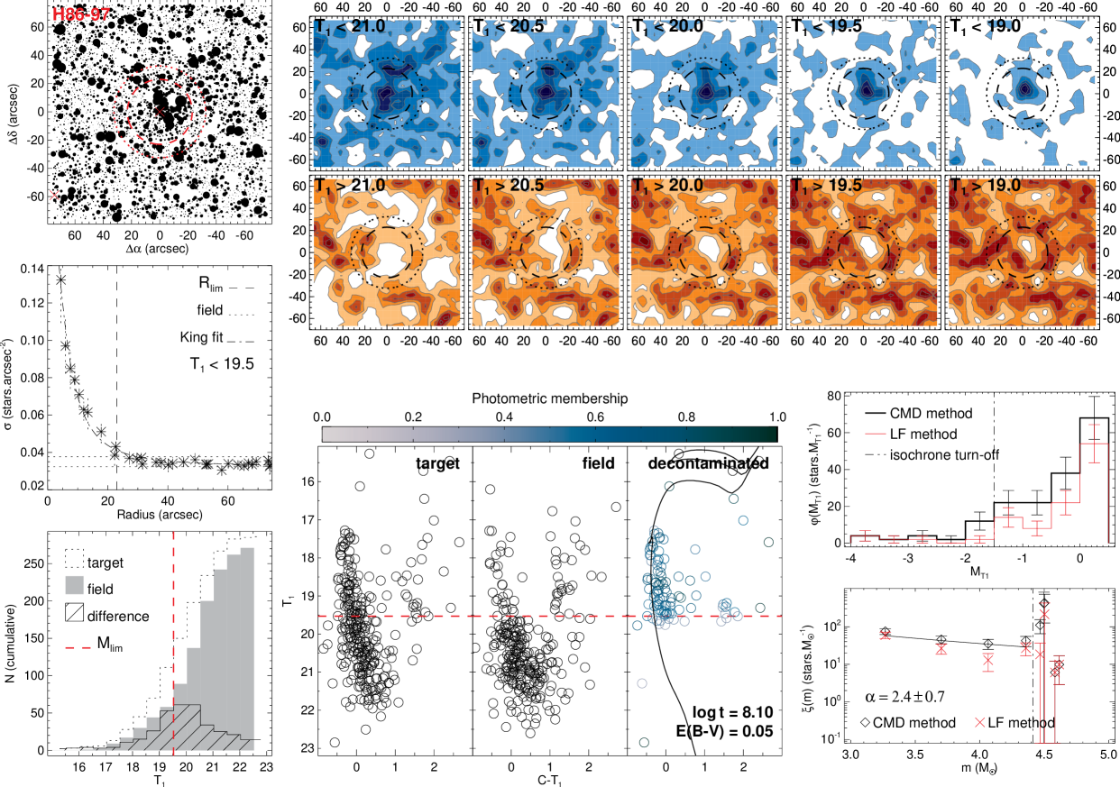
Figure 26: H86-97 analysis charts. Panels are the same as in Fig. 20

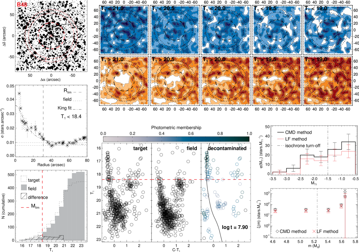
Figure 27: B48 analysis charts. Panels are the same as in Fig. 20

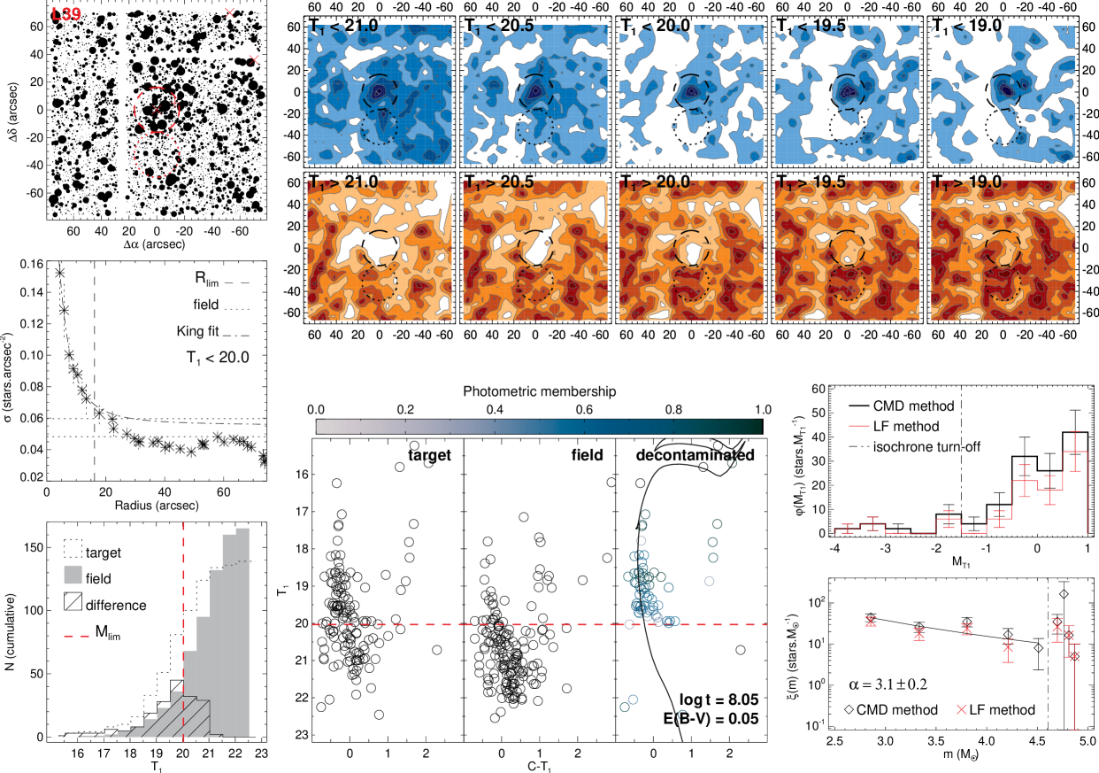
Figure 28: L39 analysis charts. Panels are the same as in Fig. 20

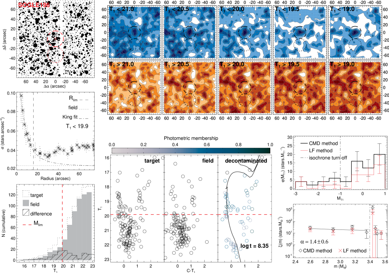
Figure 29: SOGLE196 analysis charts. Panels are the same as in Fig. 20

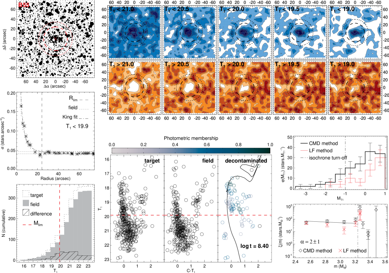
Figure 30: B55 analysis charts. Panels are the same as in Fig. 20

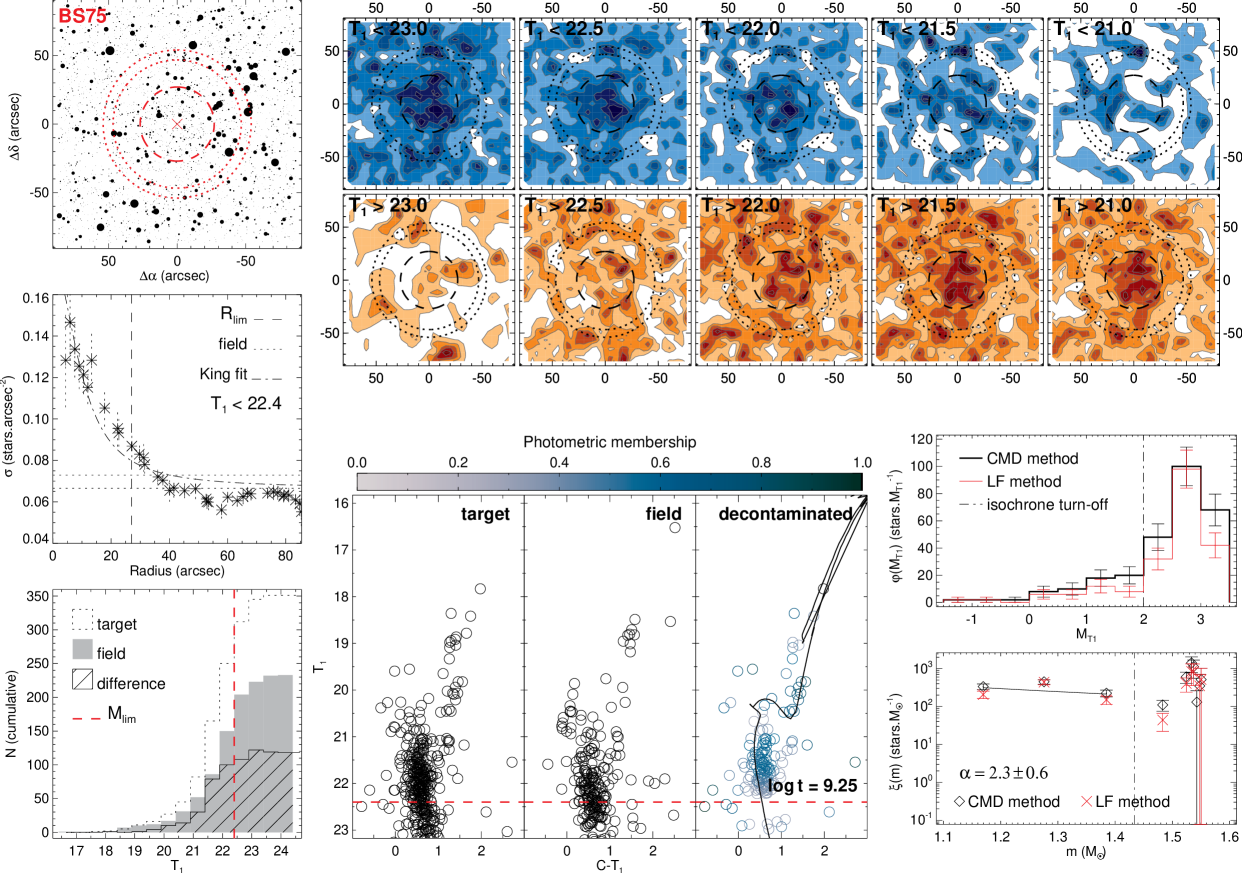
Figure 31: BS75 analysis charts. Panels are the same as in Fig. 20

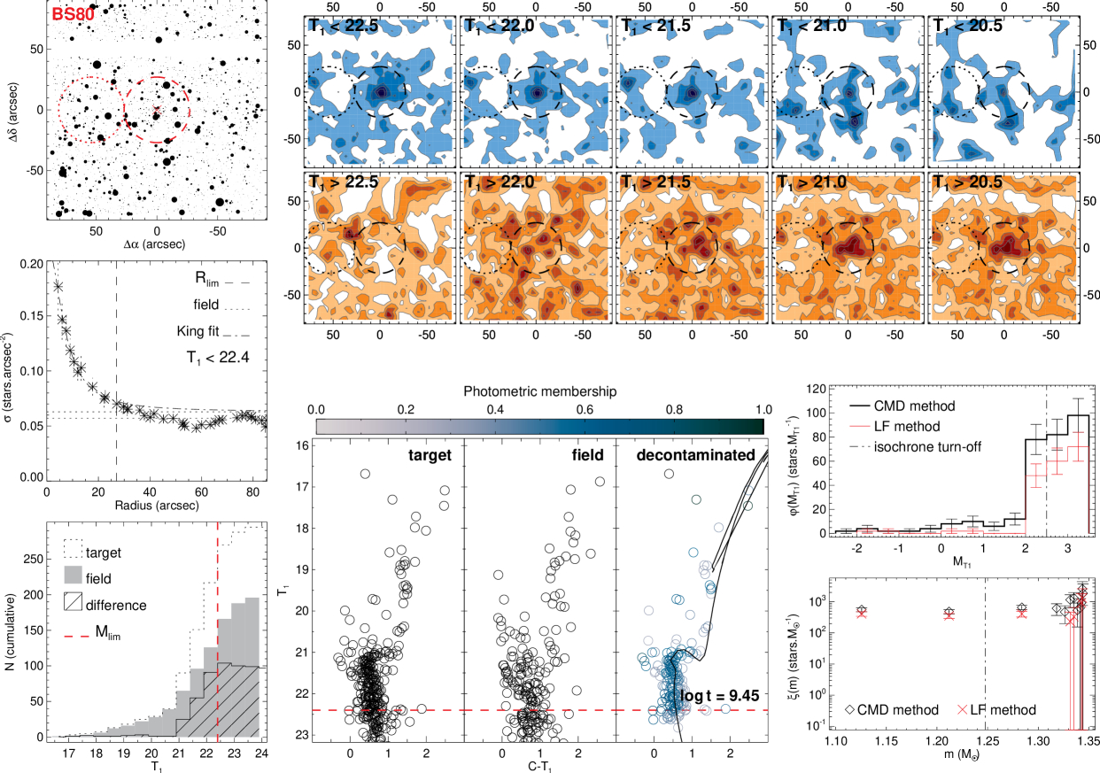
Figure 32: BS80 analysis charts. Panels are the same as in Fig. 20

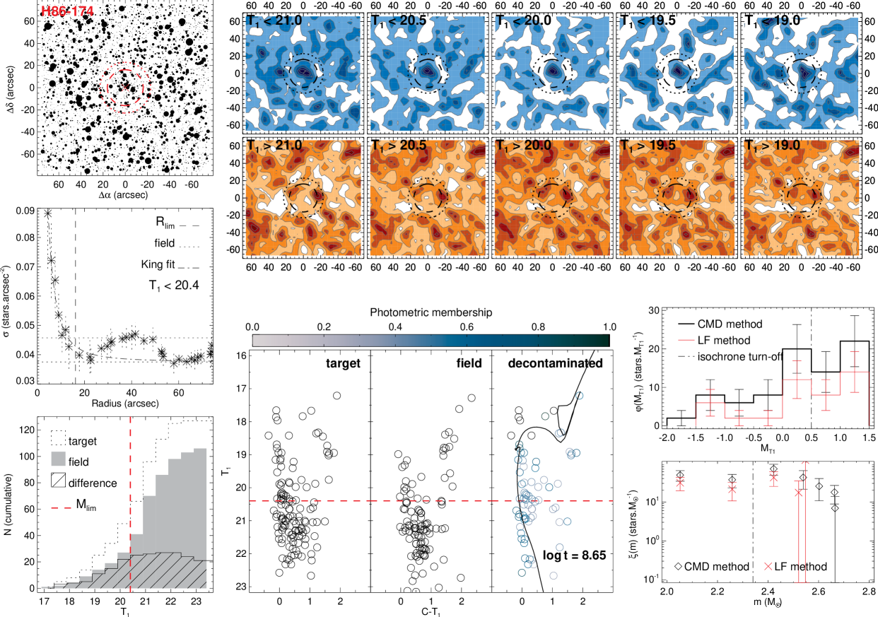
Figure 33: H86-174 analysis charts. Panels are the same as in Fig. 20

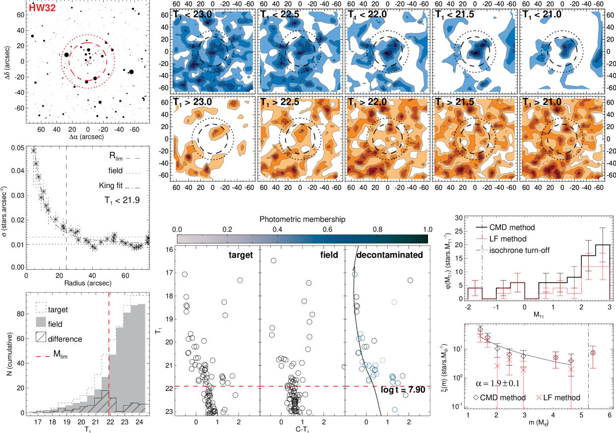
Figure 34: HW32 analysis charts. Panels are the same as in Fig. 20

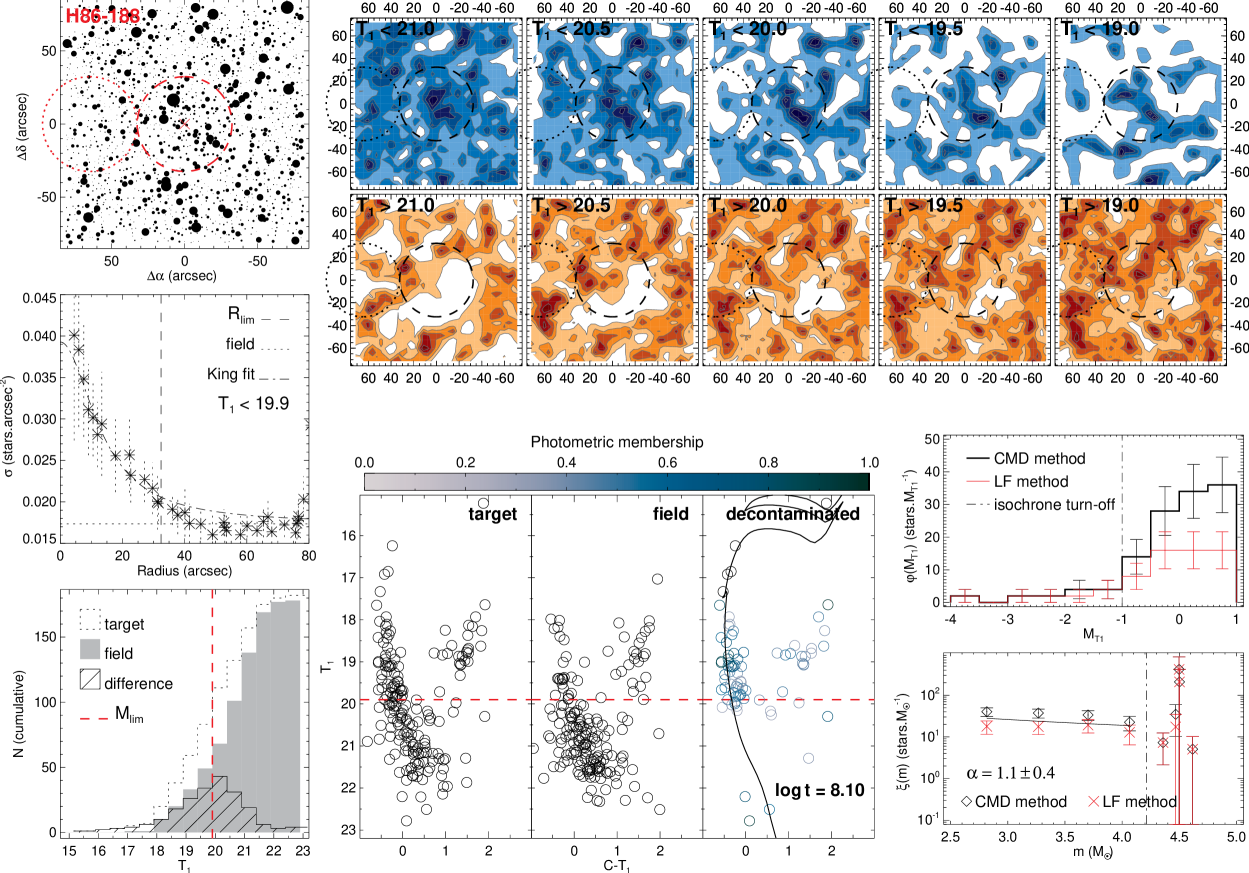
Figure 35: H86-188 analysis charts. Panels are the same as in Fig. 20

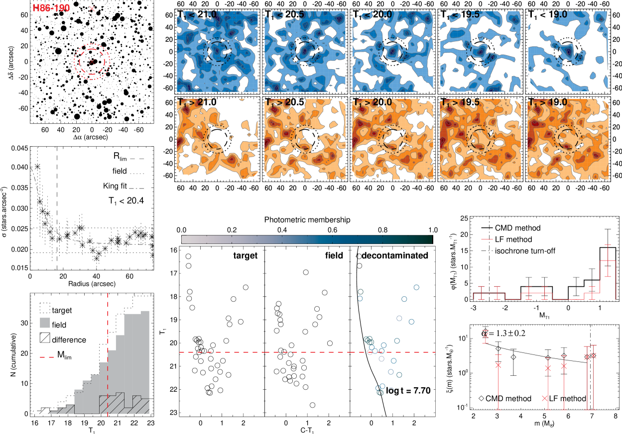
Figure 36: H86-190 analysis charts. Panels are the same as in Fig. 20

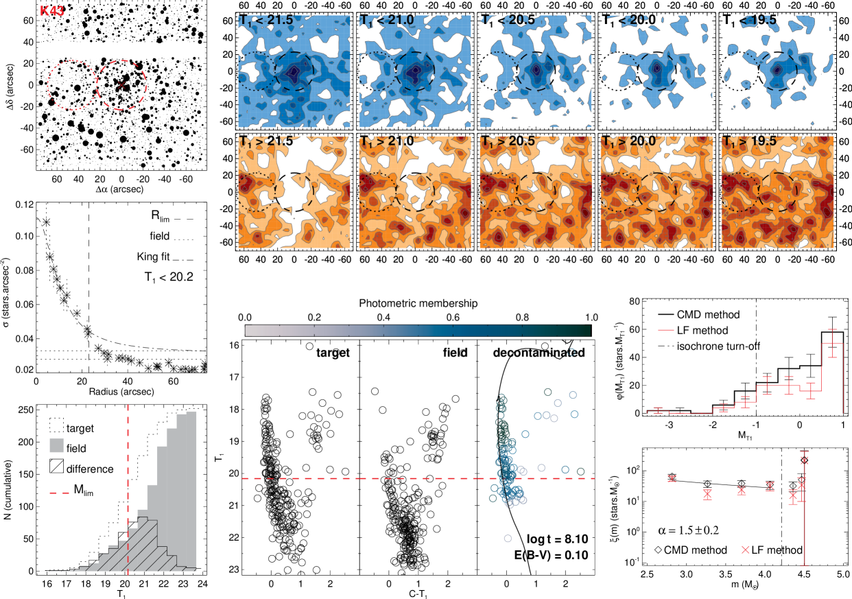
Figure 37: K43 analysis charts. Panels are the same as in Fig. 20

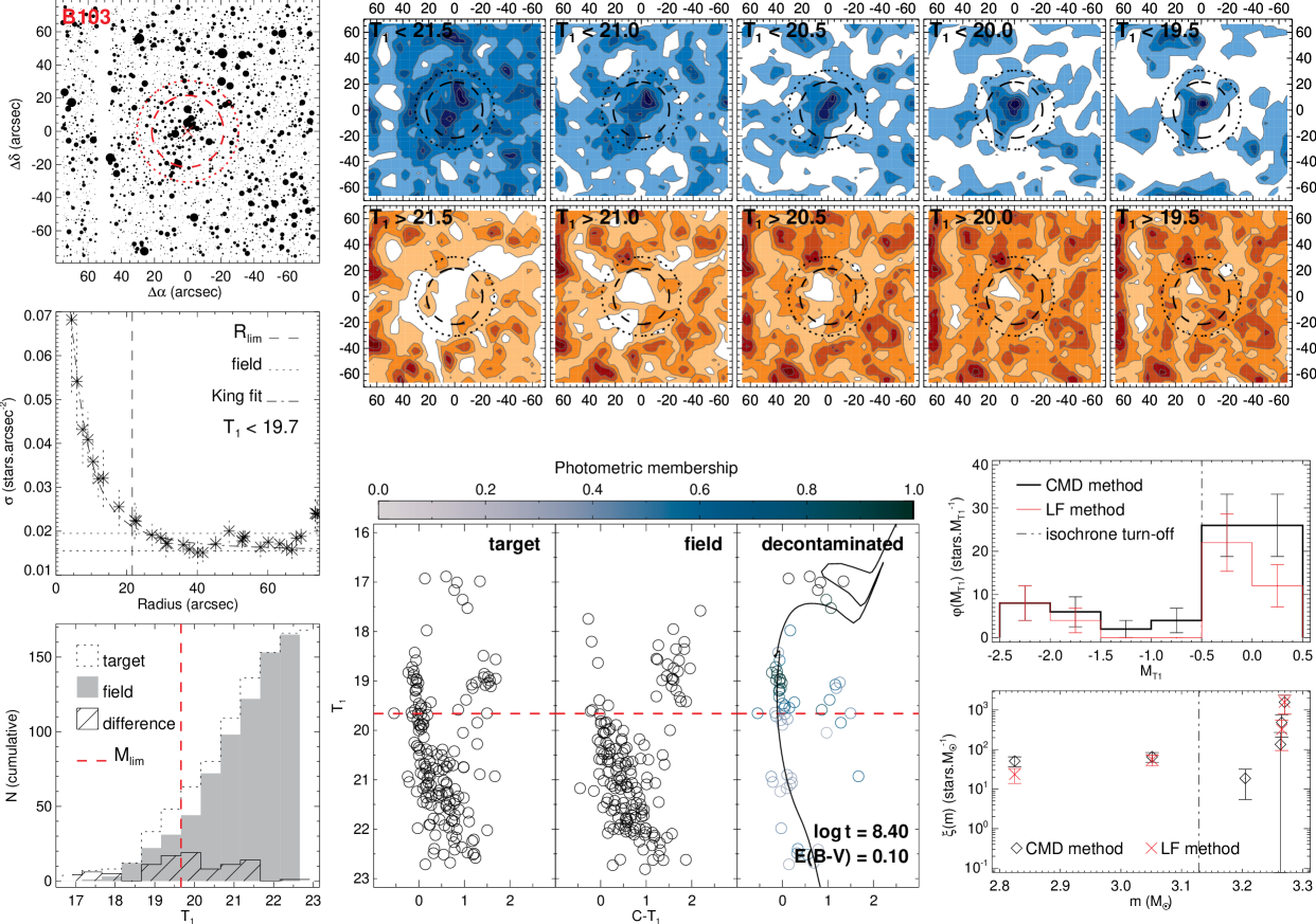
Figure 38: B103 analysis charts. Panels are the same as in Fig. 20

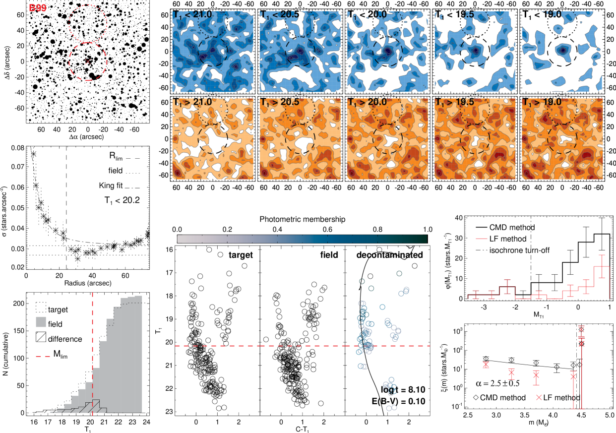
Figure 39: B99 analysis charts. Panels are the same as in Fig. 20

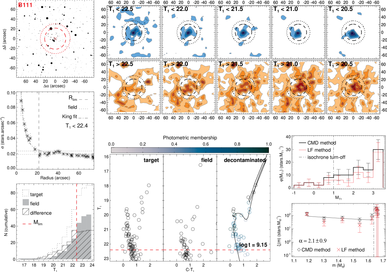
Figure 40: B111 analysis charts. Panels are the same as in Fig. 20

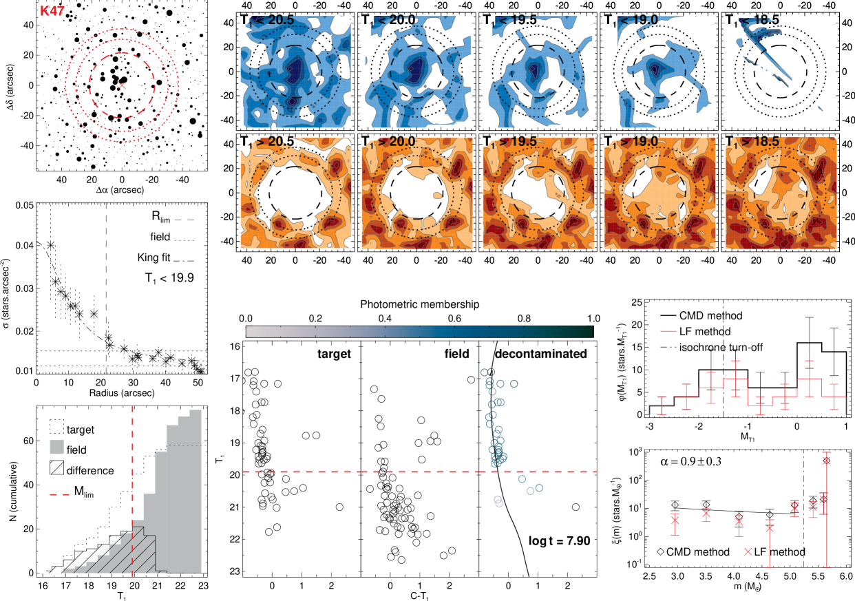
Figure 41: K47 analysis charts. Panels are the same as in Fig. 20

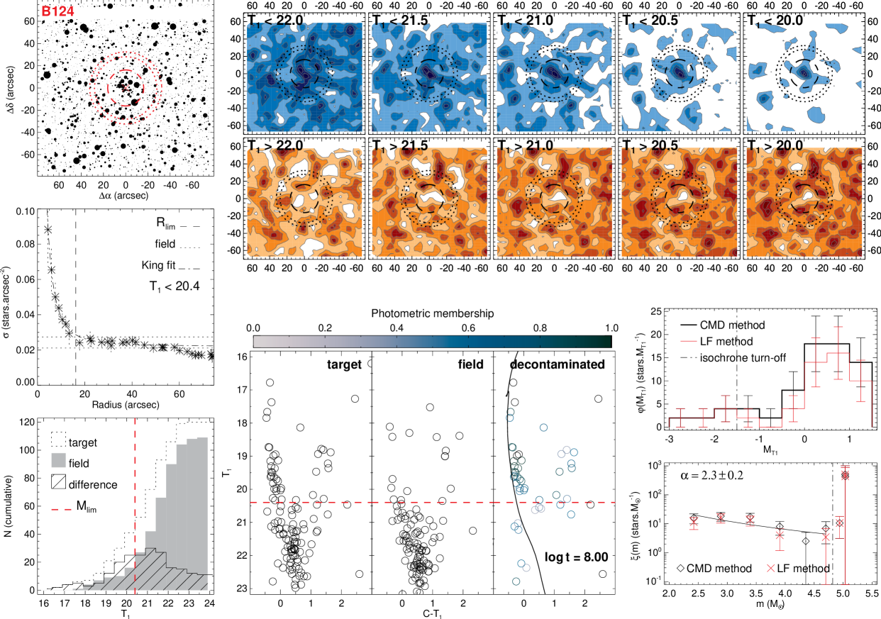
Figure 42: B124 analysis charts. Panels are the same as in Fig. 20

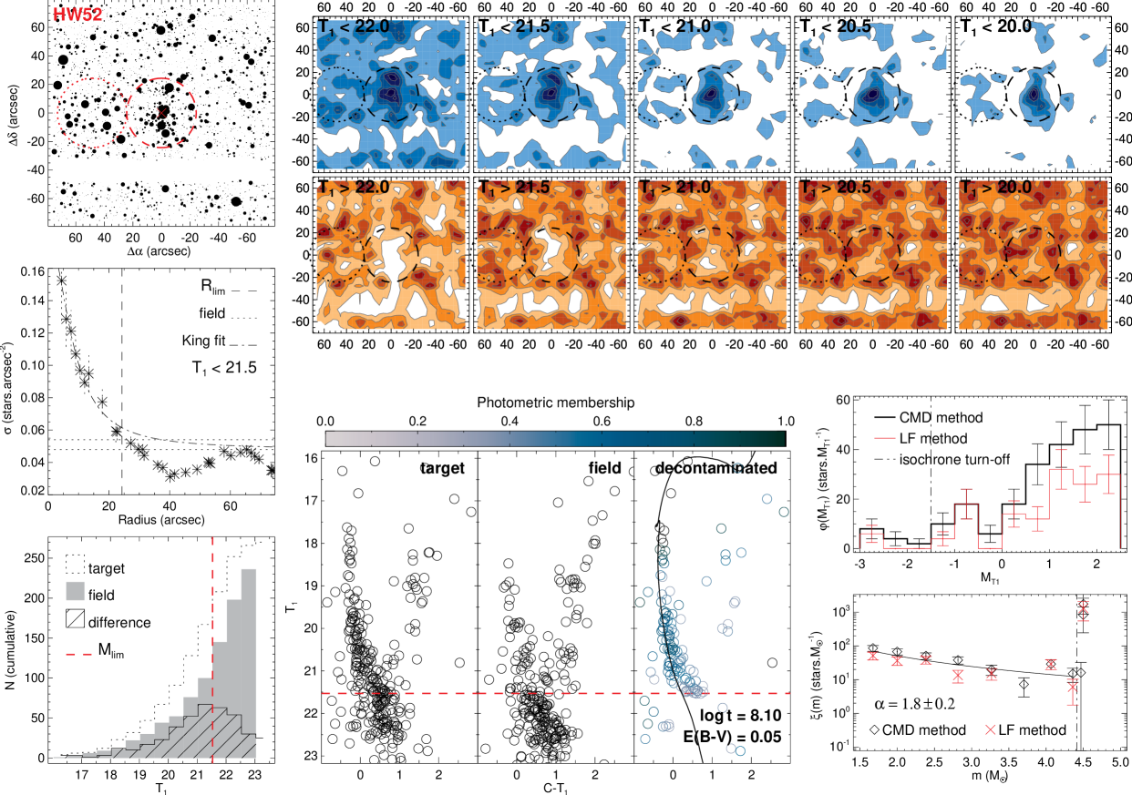
Figure 43: HW52 analysis charts. Panels are the same as in Fig. 20

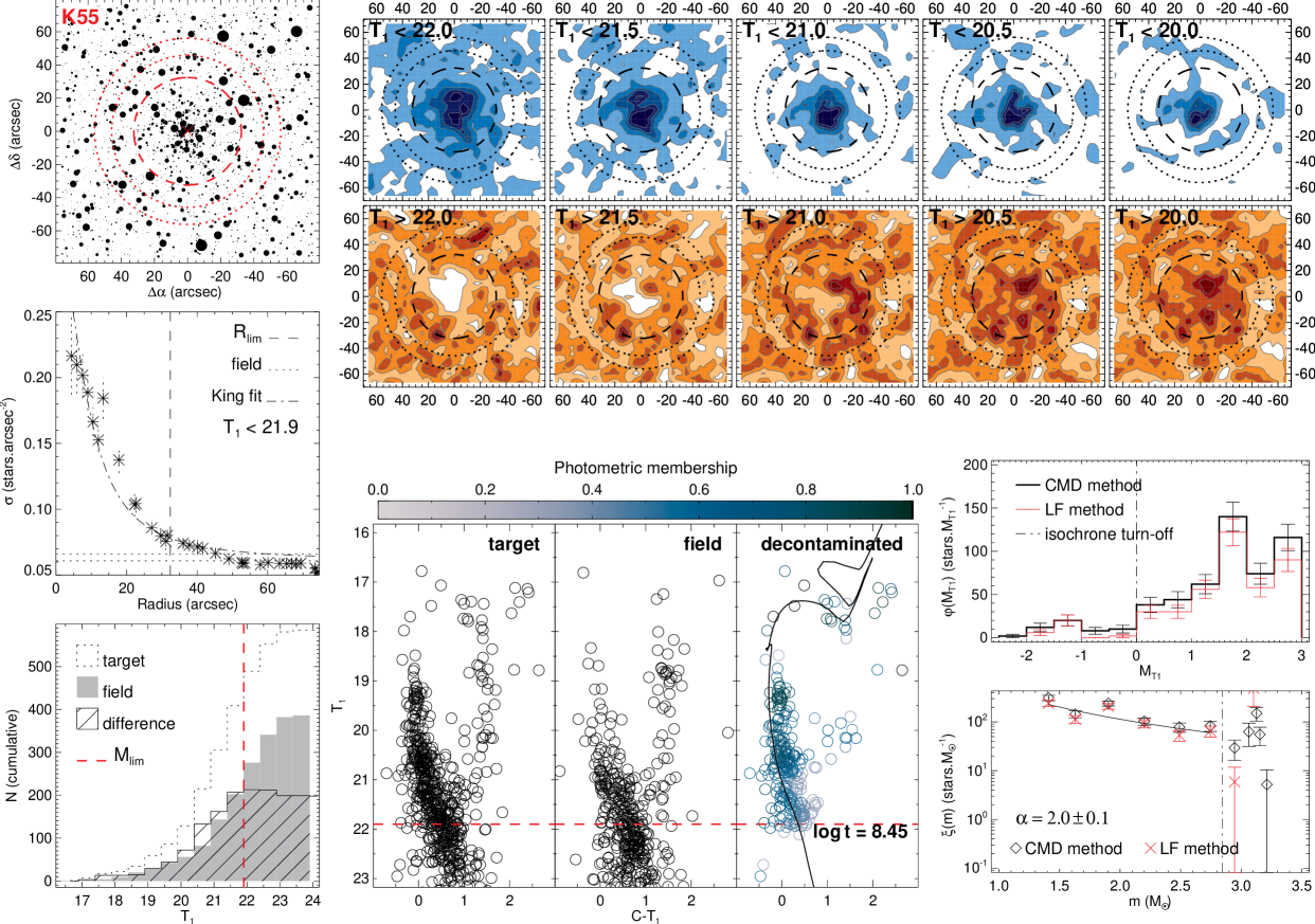
Figure 44: K55 analysis charts. Panels are the same as in Fig. 20

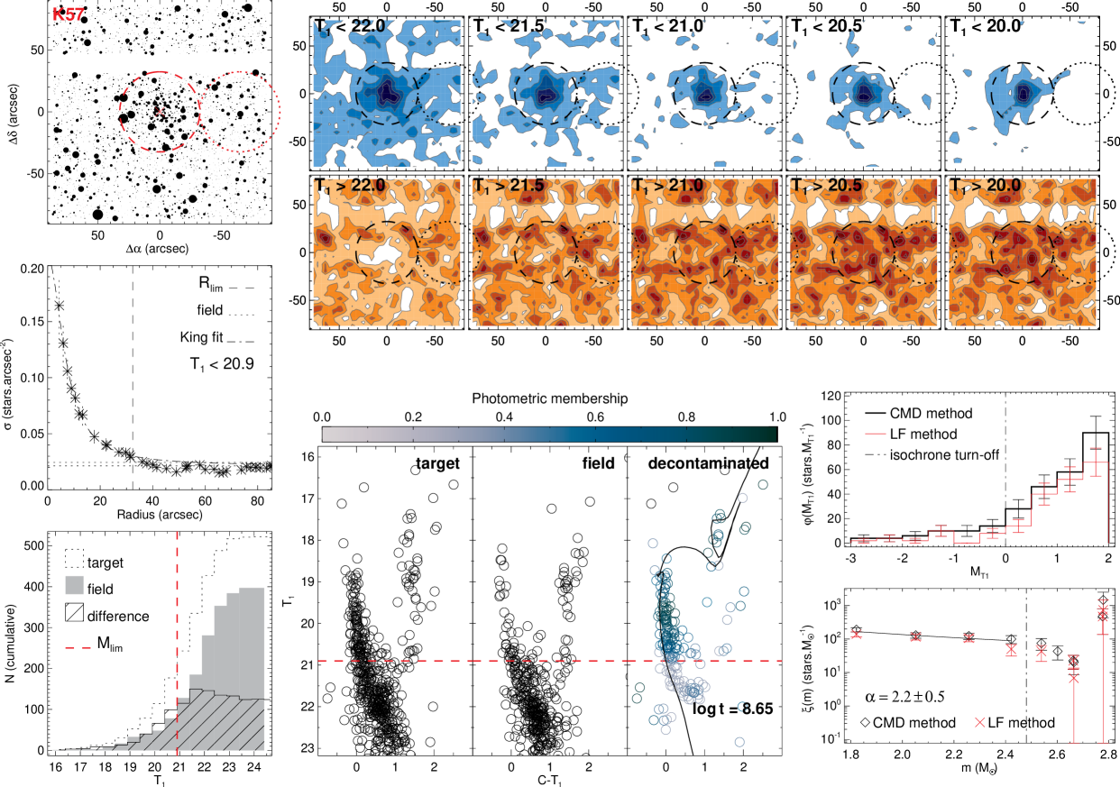
Figure 45: K57 analysis charts. Panels are the same as in Fig. 20

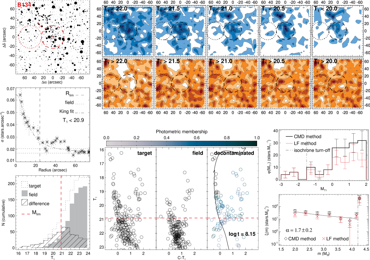
Figure 46: B134 analysis charts. Panels are the same as in Fig. 20

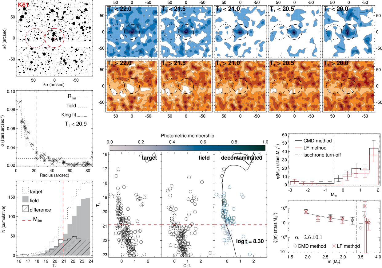
Figure 47: K61 analysis charts. Panels are the same as in Fig. 20

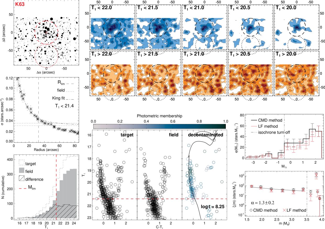
Figure 48: K63 analysis charts. Panels are the same as in Fig. 20

References

- Bica et al. (2008) Bica E., Bonatto C., Dutra C. M., Santos Jr. J. F. C., 2008, MNRAS, 389, 678
- Bica & Schmitt (1995) Bica E. L. D., Schmitt H. R., 1995, ApJS, 101, 41
- Carvalho et al. (2008) Carvalho L., Saurin T. A., Bica E., Bonatto C., Schmidt A. A., 2008, A&A, 485, 71
- Chiosi & Vallenari (2007) Chiosi E., Vallenari A., 2007, A&A, 466, 165
- Chiosi et al. (2006) Chiosi E., Vallenari A., Held E. V., Rizzi L., Moretti A., 2006, A&A, 452, 179
- Cignoni et al. (2009) Cignoni M., Sabbi E., Nota A., Tosi M., Degl’Innocenti S., Moroni P. G. P., Angeretti L., Carlson L. R., Gallagher J., Meixner M., Sirianni M., Smith L. J., 2009, AJ, 137, 3668
- de Vaucouleurs et al. (1976) de Vaucouleurs G., de Vaucouleurs A., Corwin H. G., 1976, 2nd reference catalogue of bright galaxies containing information on 4364 galaxies with reference to papers published between 1964 and 1975. University of Texas Press
- de Vaucouleurs & Freeman (1972) de Vaucouleurs G., Freeman K. C., 1972, Vistas in Astronomy, 14, 163
- Dias et al. (2010) Dias B., Coelho P., Barbuy B., Kerber L., Idiart T., 2010, A&A, 520, A85
- Elson et al. (1987) Elson R. A. W., Fall S. M., Freeman K. C., 1987, ApJ, 323, 54
- Gardiner & Hatzidimitriou (1992) Gardiner L. T., Hatzidimitriou D., 1992, MNRAS, 257, 195
- Glatt et al. (2011) Glatt K., Grebel E. K., Jordi K., Gallagher III J. S., Da Costa G., Clementini G., Tosi M., Harbeck D., Nota A., Sabbi E., Sirianni M., 2011, AJ, 142, 36
- Glatt et al. (2010) Glatt K., Grebel E. K., Koch A., 2010, A&A, 517, A50
- Glatt et al. (2008) Glatt K., Grebel E. K., Sabbi E., Gallagher III J. S., Nota A., Sirianni M., Clementini G., Tosi M., Harbeck D., Koch A., Kayser A., Da Costa G., 2008, AJ, 136, 1703
- Gouliermis et al. (2004) Gouliermis D., Keller S. C., Kontizas M., Kontizas E., Bellas-Velidis I., 2004, A&A, 416, 137
- Hindman (1967) Hindman J. V., 1967, Australian Journal of Physics, 20, 147
- Hunter et al. (2003) Hunter D. A., Elmegreen B. G., Dupuy T. J., Mortonson M., 2003, AJ, 126, 1836
- King (1962) King I., 1962, AJ, 67, 471
- Kontizas et al. (1982) Kontizas M., Danezis E., Kontizas E., 1982, A&AS, 49, 1
- Kroupa (2001) Kroupa P., 2001, MNRAS, 322, 231
- Kruijssen (2009) Kruijssen J. M. D., 2009, A&A, 507, 1409
- Lada & Lada (2003) Lada C. J., Lada E. A., 2003, ARA&A, 41, 57
- Mackey & Gilmore (2003) Mackey A. D., Gilmore G. F., 2003, MNRAS, 338, 120
- Maia et al. (2010) Maia F. F. S., Corradi W. J. B., Santos Jr. J. F. C., 2010, MNRAS, 407, 1875
- Marigo et al. (2008) Marigo P., Girardi L., Bressan A., Groenewegen M. A. T., Silva L., Granato G. L., 2008, A&A, 482, 883
- Massey et al. (1995) Massey P., Lang C. C., Degioia-Eastwood K., Garmany C. D., 1995, ApJ, 438, 188
- Mighell et al. (1998) Mighell K. J., Sarajedini A., French R. S., 1998, AJ, 116, 2395
- Piatti (2011a) Piatti A. E., 2011a, MNRAS, 416, L89
- Piatti (2011b) Piatti A. E., 2011b, MNRAS, 418, L69
- Piatti (2012) Piatti A. E., 2012, MNRAS, 422, 1109
- Piatti & Bica (2012) Piatti A. E., Bica E., 2012, MNRAS, 425, 3085
- Piatti et al. (2011) Piatti A. E., Clariá J. J., Bica E., Geisler D., Ahumada A. V., Girardi L., 2011, MNRAS, 417, 1559
- Pietrzynski & Udalski (1999) Pietrzynski G., Udalski A., 1999, Acta Astron., 49, 157
- Rich et al. (2000) Rich R. M., Shara M., Fall S. M., Zurek D., 2000, AJ, 119, 197
- Rochau et al. (2007) Rochau B., Gouliermis D. A., Brandner W., Dolphin A. E., Henning T., 2007, ApJ, 664, 322
- Sabbi et al. (2008) Sabbi E., Sirianni M., Nota A., Tosi M., Gallagher J., Smith L. J., Angeretti L., Meixner M., Oey M. S., Walterbos R., Pasquali A., 2008, AJ, 135, 173
- Salpeter (1955) Salpeter E. E., 1955, ApJ, 121, 161
- Schmalzl et al. (2008) Schmalzl M., Gouliermis D. A., Dolphin A. E., Henning T., 2008, ApJ, 681, 290
- Sirianni et al. (2002) Sirianni M., Nota A., De Marchi G., Leitherer C., Clampin M., 2002, ApJ, 579, 275
- Westerlund (1997) Westerlund B. E., 1997, The Magellanic Clouds. Cambridge U Press
- Zaritsky et al. (2000) Zaritsky D., Harris J., Grebel E. K., Thompson I. B., 2000, ApJ, 534, L53