Abstract

A mathematical model for fluid and solute transport in peritoneal dialysis is constructed. The model is based on a three-component nonlinear system of two-dimensional partial differential equations for fluid, glucose and albumin transport with the relevant boundary and initial conditions. Its aim is to model ultrafiltration of water combined with inflow of glucose to the tissue and removal of albumin from the body during dialysis, and it does this by finding the spatial distributions of glucose and albumin concentrations and hydrostatic pressure. The model is developed in one spatial dimension approximation and a governing equation for each of the variables is derived from physical principles. Under certain assumptions the model are simplified with the aim of obtaining exact formulae for spatially non-uniform steady-state solutions. As the result, the exact formulae for the fluid fluxes from blood to tissue and across the tissue are constructed together with two linear autonomous ODEs for glucose and albumin concentrations in the tissue. The obtained analytical results are checked for their applicability for the description of fluid-glucose-albumin transport during peritoneal dialysis.

Keywords: fluid transport; transport in peritoneal dialysis; nonlinear differential equation; steady-state solution

1 Introduction

Peritoneal dialysis is a life saving treatment for chronic patients with end stage renal disease (Gokal R and Nolph 1994). The peritoneal cavity, an empty space that separates bowels, abdominal muscles and other organs in the abdominal cavity, is applied as a container for dialysis fluid, which is infused there through a permanent catheter and left in the cavity for a few hours. During this time small metabolites (urea, creatinine) and other uremic toxins diffuse from blood that perfuses the tissue layers close to the peritoneal cavity to the dialysis fluid, and finally are removed together with the drained fluid. The treatment cycle (infusion, dwell, drainage) is repeated several times every day. The peritoneal transport occurs between dialysis fluid in the peritoneal cavity and blood passing down the capillaries in tissue surrounding the peritoneal cavity. The capillaries are distributed within the tissue at different distance from the tissue surface in contact with dialysis fluid. The solutes, which are transported between blood and dialysis fluid, have to cross two transport barriers: the capillary wall and a tissue layer (Flessner 2006). Typically, many solutes are transported from blood to dialysate, but some solutes such as for example an osmotic agent (it is typically glucose), that is present in high concentration in dialysis fluid, are transported in the opposite direction, i.e., to the blood. This kind of transport system happens also in other medical treatments, as local delivery of anticancer medications, and some experimental or natural physiological phenomena (see below). Typically, to take into account spatial properties of these systems, a distributed approach is applied. The first applications of the distributed model were limited to the diffusive transport of gases between blood and artificial gas pockets within the body (Piiper et al 1962), between subcutaneous pockets and blood (Van Liew 1968, Collins 1981), and the transport of heat and solutes between blood and tissue (Perl 1963, Pearl 1962). The applications of the distributed approach for modeling of the diffusive transport of small solutes include the description of the transport from cerebrospinal fluid to the brain (Patlak 1975), delivery of drugs to the human bladder during intravesical chemotherapy, and drug delivery from the skin surface to the dermis in normal and cancer tissue (Gupta et al 1995; Wientjes et al. 1993; Wientjes et al. 1991). Finally, the distributed approach was also proposed for the theoretical description of fluid and solute transport in solid tumors (Baxter and Jain 1989, 1990, 1991). The mathematical description of these systems was obtained using partial differential equations based on the simplification that capillaries are homogeneously distributed within the tissue. Experimental evidence confirmed the good applicability of such models (see, for example, the papers (Waniewski et al. 1996a,1996b; Smit et al 2004a; Flessner 2006; Parikova et al. 2006; Waniewski et al. 2007; Stachowska-Pietka et al. 2012) and references therein).

An important objective of peritoneal dialysis is to remove excess water from the patient (Gokal R and Nolph 1994). The typical values of the water ultrafiltration measured during peritoneal dialysis are $10-20$ $mL/min$ (Heimbürger et al. 1992; Waniewski et al. 1996a,1996b; Smit et al 2004a; Smit et al 2004b). This is gained by inducing osmotic pressure in dialysis fluid by adding a solute (called osmotic agent) in high concentration. The most often used osmotic agent is glucose. This medical application of high osmotic pressure is unique for peritoneal dialysis. The flow of water from blood across the tissue to dialysis fluid in the peritoneal cavity carries solutes of different size, including large proteins, and adds a convective component to their diffusive transport.

Mathematical description of fluid and solute transport between blood and dialysis fluid in the peritoneal cavity has not been formulated fully yet, in spite of the well known basic physical laws for such transport. The complexity of the peritoneal fluid transport modelling comes mainly from the fact that, whereas diffusive transport of small solutes is linear, process of water removal during peritoneal dialysis by osmosis is nonlinear. A first formulation of the general distributed model for combined solute and fluid transport was proposed by Flessner et al. (1984) and applied later for the description of the peritoneal transport of small molecules (Flessner et al. 1985).

The next attempt to model fluid and solute transport did not result in a satisfactory description. It was assumed in that model that mesothelium is a very efficient osmotic barrier for glucose with the same transport characteristics as endothelium (Seams et al, 1990). The assumption resulted in negative interstitial hydrostatic pressures during osmotically driven ultrafiltration from blood to the peritoneal cavity during peritoneal dialysis (Seams et al, 1990). This prediction was shown to contradict the experimental evidence on positive interstitial hydrostatic pressure during ultrafiltration period of peritoneal dialysis (Flessner 1994). Moreover, the mesothelium being a very permeable layer cannot provide enough resistance to small solute transport to be an osmotic barrier for such solutes as glucose (Flessner 1994; Czyzewska et al. 2000; Flessner 2006).

Recent mathematical, theoretical and numerical studies introduced new concepts on peritoneal transport and yielded better description of particular processes such as pure water transport, combined osmotic fluid flow and small solute transport, or water and proteins transport (Flessner 2001, Cherniha and Waniewski 2005; Stachowska-Pietka et al. 2006,2007; Cherniha et al. 2007; Waniewski et al.2007, Waniewski et al.2009). The recent study (Stachowska-Pietka et al. 2012) addresses again a combined transport of fluid (water) and several small solutes. However, the problem of a combined description of osmotic ultrafiltration to the peritoneal cavity, absorption of osmotic agent from the peritoneal cavity and leak of macromolecules (e.g., albumin) from blood to the peritoneal cavity has not been addressed yet. Therefore, we present here an extended model for these phenomena and investigate its mathematical structure. In particular, the present study is aimed on investigation of some basic questions concerning the role of various transport components, as osmotic and oncotic gradients and hydrostatic pressure gradient. It should be stressed that the oncotic gradient leading to leak of macromolecules from blood to the peritoneal cavity has opposite sign to the osmotic gradient, hence, their combination may lead to new effects, which do not arise in the case of the simplified models mentioned above.

The paper is organized as follows. In section 2, a mathematical model of glucose and albumin transport in peritoneal dialysis is constructed. In section 3, non-uniform steady-state solutions of the model are constructed and their properties are investigated. Moreover, these solutions are tested for the real parameters that represent clinical treatments of peritoneal dialysis. The results are compared with those derived by numerical simulations for simplified models (Cherniha et al. 2007, Waniewski et al. 2007). Finally, we present some conclusions and discussion in the last section.

2. Mathematical model

Here we present new model of fluid and solute transport in peritoneal dialysis. The model is developed in one spatial dimension with $x=0$ (see the vertical orange line in Fig.1) representing the boundary of the peritoneal cavity and $x=L$ representing the end of the tissue surrounding the peritoneal cavity, see (Stachowska-Pietka et al. 2012) for the discussion of the assumptions involved in this approach.

The mathematical description of transport processes within the tissue consists in local balance of fluid volume and solute mass. For incompressible fluid, the change of volume may occur only due to elasticity of the tissue. The fractional fluid void volume, i.e. the volume occupied by the fluid in the interstitium (the rest of the tissue being cells and macromolecules forming the solid structure of the interstitium) expressed per one unit volume of the whole tissue, is denoted by $\nu(t,x)$, and its time evolution is described as:

$${{\partial\nu}\over{\partial t}}=-{{\partial j_{U}}\over{\partial x}}+q_{U}-q_{l}$$ (1)

where $j_{U}(t,x)$ is the volumetric fluid flux across the tissue (ultrafiltration), $q_{U}(t,x)$ is the density of volumetric fluid flux from blood capillaries to the tissue, and $q_{l}$ is the density of volumetric fluid flux from the tissue to the lymphatic vessels (hereafter we assume that it is a known positive constant, nevertheless it can be also a function of hydrostatic pressure ( Stachowska et al, 2006, 2012)). Similarly to many distributed models, our model involves the spreading of the source within the whole tissue as an approximation to the discrete structure of blood and lymphatic capillaries.

The independent variables are time $t$ and the distance $x$ within the tissue from the tissue surface in contact with dialysis fluid in the direction perpendicular to this surface (flat geometry of the tissue is here assumed with finite width, see below). The solutes, glucose and albumin, are distributed only within the interstitial fluid (or part of it, see below), and their concentrations in this fluid are denoted by $C_{G}(t,x)$ and $C_{A}(t,x)$, respectively. The equation that describes the local changes of glucose amount in the tissue, $\nu C_{G}$, is:

$${{\partial(\nu C_{G})}\over{\partial t}}=-{{\partial j_{G}}\over{\partial x}}+q_{G},$$ (2)

where $j_{G}(t,x)$ is glucose flux through the tissue, and $q_{G}(t,x)$ is the density of glucose flux from blood. The cellular uptake of absorbed glucose is not taken into account in equation (2) because this process leads to a small correction to the bulk absorption of glucose to the capillaries. So, we neglect the intracellular changes that were noted experimentally (Zakaria et al. 2000).

Similarly, the equation that describes the local changes of albumin amount in the tissue, $\alpha\nu C_{A}$, is:

$${{\partial(\alpha\nu C_{A})}\over{\partial t}}=-{{\partial j_{A}}\over{\partial x}}+q_{A},$$ (3)

where $j_{A}(t,x)$ is albumin flux through the tissue, $q_{A}(t,x)$ is the density of albumin flux from blood. The coefficient $\alpha<1$ takes into account that only a part of the fractional fluid void volume $\nu$ that is available for fluid, is accessible for albumin because of its large molecular size (Flessner 2001; Stachowska-Pietka et al. 2007). In other words, the inclusion of the term $\alpha\nu$ in (3) implies that $C_{A}(t,x)$ is the concentration of albumin in that part of the interstitium across which the albumin molecules can pass. In the general case, equation (3) involves a new fluid void volume function $\nu_{A}(t,x)$, which depends on the hydrostatic pressure similarly to the function $\nu$ (see below) and satisfies the inequality $\nu_{A}<\nu$. Hereafter we set $\nu_{A}=\alpha\nu$ for simplicity.

The flows of fluid and solutes through the tissue are described according to linear non-equilibrium thermodynamics. Osmotic pressure of glucose and oncotic pressure of albumin are described by van’t Hoff law, i.e. assuming that corresponding pressures are proportional to the relevant concentrations.

The fluid flux across the tissue is generated by hydrostatic, osmotic and oncotic (i.e., osmotic pressure of large proteins) pressure gradients:

$$j_{U}=-\nu K{{\partial P}\over{\partial x}}+\sigma_{TG}\nu KRT{{\partial C_{G}}\over{\partial x}}+\sigma_{TA}\nu KRT{{\partial C_{A}}\over{\partial x}},$$ (4)

where $K$ is the hydraulic conductivity of tissue that is assumed constant for simplicity( $K$ may also depend on the pressure $P$), $R$ is the gas constant, $T$ is absolute temperature, and $\sigma_{TG}$ and $\sigma_{TA}$ are the Staverman reflection coefficients for glucose and albumin in tissue, respectively. The Staverman reflection coefficient $\sigma$ is a thermodynamic parameter and describes the effectiveness of osmotic pressure in selectively permeable membrane: if $\sigma=0$ then no osmotic pressure can be induced by this solute across the membrane, and if $\sigma=1$ the maximal theoretically possible osmotic effect can be induced (ideal semi-permeable membrane). The intermediate values of $\sigma$ represent non-ideal semipermeable membranes. The book (Currant, Katchalsky 1965) well addresses the problem of the Staverman reflection coefficients.

The density of fluid flux from blood to tissue is generated, according to Starling law, by the hydrostatic, osmotic and oncotic pressure differences between blood and tissue:

$$q_{U}=L_{p}a(P_{B}-P)-L_{p}a\sigma_{G}RT(C_{GB}-C_{G})-L_{p}a\sigma_{A}RT(C_{AB}-C_{A}),$$ (5)

where $P(t,x)$ is hydrostatic pressure, $L_{p}a$ is the hydraulic conductance of the capillary wall, $P_{B}$ is the hydrostatic pressure of blood, $C_{GB}$ and $C_{AB}$ are glucose and albumin concentrations in blood, and $\sigma_{G}$ and $\sigma_{A}$ are the Staverman reflection coefficients for glucose and albumin in the capillary wall, respectively. In contrary to other parameters, there is an unsolved problem of the values of $\sigma_{G}$ and $\sigma_{A}$. In particular, the values of $\sigma_{G}$ were found low (about $0.005-0.03$) in many experiments in contrast to some newer experimental data that suggest the values close to $0.5$ (see the discussion of this controversy in (Waniewski et al. 2009, Stachowska-Pietka et al. 2012)). We also assume that blood concentrations of glucose and albumin are constant according to the clinical and experimental data that demonstrate only negligible variation of these concentrations during peritoneal dwell of dialysis fluid (Heimburger et al. 1992). This observation is related to a quasi-continuous mode of continuous ambulatory peritoneal dialysis with fluid exchanges every few hours and was applied in most previous theoretical and numerical studies on peritoneal dialysis.

The glucose flux across the tissue is composed of diffusive component (proportional to glucose concentration gradient) and convective component (proportional to glucose concentration and fluid flux):

$$j_{G}=-\nu D_{G}{{\partial C_{G}}\over{\partial x}}+S_{TG}C_{G}j_{U}.$$ (6)

where $D_{G}$ is the diffusivity of glucose in tissue, $S_{TG}$ is the sieving coefficients of glucose in tissue. According to non-equilibrium thermodynamics, $S_{TG}=1-\sigma_{TG}$ for homogenous membrane ( Katchalsky, Currant 1965).

The density of glucose flux between blood and the tissue describes the number of moles of glucose per unit total volume of tissue per unit time that move between blood and tissue. It has diffusive component (proportional to the difference of glucose concentration in blood, $C_{GB}$, and glucose concentration in tissue, $C_{G}$), convective component (proportional to the density of fluid flow from blood to tissue, $q_{U}$) and the component that represents lymphatic absorption of solutes (proportional to the density of volumetric lymph flux, $q_{l}$):

$$q_{G}=p_{G}a(C_{GB}-C_{G})+S_{G}q_{U}C_{G}-q_{l}C_{G}.$$ (7)

where $p_{G}a$ is the diffusive permeability of the capillary wall for glucose.

In a similar way, the albumin flux across the tissue, $j_{A}(t,x)$, and the density of albumin flux to tissue, $q_{A}(t,x)$, can be described as:

$$j_{A}=-\alpha\nu D_{A}{{\partial C_{A}}\over{\partial x}}+S_{TA}C_{A}j_{U},$$ (8)

$$q_{A}=p_{A}a(C_{AB}-C_{A})+S_{A}q_{U}C_{A}-q_{l}C_{A}.$$ (9)

where $S_{TA}=1-\sigma_{TA}$ is the sieving coefficient of albumin in tissue, $S_{A}=1-\sigma_{A}$ is the sieving coefficient of glucose and albumin in the capillary wall, $D_{A}$ is the diffusivity of albumin in tissue, and $p_{A}a$ is the diffusive permeability of the capillary wall for albumin.

The typical values of the model parameters are listed in Table 1.

Equations (1)-(3) together with equations (4)-(9) for flows form a system of three nonlinear partial differential equations with four variables: $\nu,P,C_{A}$, and $C_{G}$. Therefore, an additional, constitutive, equation is necessary, and this is the equation describing how fractional fluid void volume, $\nu$, depends on interstitial pressure, $P$. This dependence can be established using data from experimental studies (Stachowska-Pietka et al. 2006). It turns out that

$$\nu=F(P),$$ (10)

where $F$ is a monotonically non-decreasing bounded function with the limits: $F\to\nu_{\min}$ if $P\to P_{\min}$ and $F\to\nu_{\max}$ if $P\to P_{\max}$ (particularly, one may take $P_{\min}=-\infty,\ P_{\max}=\infty$). Here $\nu_{\min}<1$ and $\nu_{max}<1$ are empirically measured constants. For example, the following analytical form for the function $F$ based on experimental data taken from (Zakaria et al. 1999)

$$\nu(P)=\nu_{\min}+\frac{\nu_{\max}-\nu_{\min}}{1+\left(\frac{\nu_{\max}-\nu_{\min}}{\nu_{0}-\nu_{\min}}-1\right)e^{-bP}},\quad b>0$$

was used in (Stachowska-Pietka et al. 2006; Cherniha et al. 2007).

Boundary conditions for a tissue layer of width $L$ impermeable at $x=L$ and in contact with dialysis fluid at $x=0$ are:

$$x=0:\ P=P_{D},\quad C_{G}=C_{GD},\quad C_{A}=C_{AD}$$ (11)

$$x=L:\ {{\partial P}\over{\partial x}}=0,\quad{{\partial C_{G}}\over{\partial x}}=0,\quad{{\partial C_{A}}\over{\partial x}}=0.$$ (12)

Generally speaking, intraperitoneal pressure $P_{D}$, glucose $C_{GD}$ and albumin $C_{AD}$ concentrations in the peritoneal cavity may depend on time. However, experimental data and theoretical studies suggest that they change at low rate compared to the rate of transport processes in the tissue (Stachowska-Pietka et al. 2006,2007;Waniewski 2007). Therefore, we may assume that $P_{D}$, $C_{GD}$ and $C_{AD}$ are constant for some time period and assess the steady-state solution for these particular boundary conditions that may be considered as approximated quasi steady-state solution for the full model of peritoneal dialysis with time-dependent boundary conditions. This approximation was applied previously for the model with variable boundary conditions for small solutes (as glucose) and water transport (but without proteins, as albumin), see (Dedrick 1981; Flessner et al.1984, Flessner et al. 1985; Seames et al. 1990; Stachowska-Pietka et al. 2006, Stachowska-Pietka et al. 2007; Waniewski 2001, 2002; Waniewski et al. 2009).

Initial conditions describe equilibrium within the tissue without any contact with dialysis fluid:

$$t=0:\ P=P^{*},\ C_{G}=C^{*}_{G},\ C_{A}=C^{*}_{A},$$ (13)

where $P^{*},\ C^{*}_{G},$ and $C^{*}_{A}$ are some non-negative values, which will be estimated below.

Note that equations (1)-(10) can be united into three nonlinear partial differential equations (PDEs) for hydrostatic pressure $P(t,x)$, glucose concentration $C_{G}(t,x)$ and albumin concentration $C_{A}(t,x)$. Thus, these three PDEs together with boundary and initial conditions (11)-(13) form a nonlinear boundary-value problem. Possible values of the parameters arising in this problem are presented in Table 1 (see the relevant comments in Section 4).

The fluid flux $j_{U}(t,x)$ at $x=0$ describes the net ultrafiltration flow, i.e., the exchange of fluid between the tissue and the peritoneal cavity across the peritoneal surface and therefore directly the efficiency of removal of water during peritoneal dialysis. The assessment of ultrafiltration flow is important from practical point of view because the low values of this flow in some patients indicate that some problems with osmotic fluid removal occur, which may finally result in the failure of the therapy (Parikova 2006).

3. Steady-state solutions of the model and their applications

First of all, we consider the special case, with tissue in its physiological state without dialysis, and, therefore, no transport to the peritoneal cavity occurs. In this case the boundary conditions at $x=0$ given by Eq. (11) are replaced by zero Neumann conditions, and the steady-state solution can be easily found because it does not depend on $x$. In fact solving algebraic equations

$$q_{U}-q_{l}=0,\quad q_{G}=0,\quad q_{A}=0,$$ (14)

one easily obtains the spatially uniform steady-state solution

$$\begin{array}[]{l}\vskip 6.0pt plus 2.0pt minus 2.0ptC_{G}^{*}=\frac{p_{G}a}{p_{G}a+\sigma_{G}q_{l}}C_{GB}\\ \vskip 6.0pt plus 2.0pt minus 2.0ptC_{A}^{*}=\frac{p_{A}a}{p_{A}a+\sigma_{A}q_{l}}C_{AB}\\ P^{*}=P_{B}-q_{l}\Bigl{(}\frac{1}{L_{p}a}+RT\Bigl{(}\frac{\sigma_{G}^{2}C_{GB}}{p_{G}a+\sigma_{G}q_{l}}+\frac{\sigma_{A}^{2}C_{AB}}{p_{A}a+\sigma_{A}q_{l}}\Bigr{)}\Bigr{)}.\end{array}$$ (15)

In the case $q_{l}=0$, i.e., zero flux from the tissue to the lymphatic vessels, formulae (15) produce

$$C_{G}^{*}=C_{GB},\quad C_{A}^{*}=C_{AB},\quad P^{*}=P_{B},$$ (16)

otherwise

$$C_{G}^{*}<C_{GB},\quad C_{A}^{*}<C_{AB},\quad P^{*}<P_{B}.$$ (17)

This uniform solution describes the system in equilibrium if no dialysis is performed, and therefore we may use the values $P^{*},\ C^{*}_{G},$ and $C^{*}_{A}$ calculated above as the initial profile for simulation of the transport processes after the initiation of dialysis (see formulae (13) ).

To find spatially non-uniform steady-state solutions, we reduce Eqs. (1)-(3) to an equivalent form by introducing scaled non-dimensional independent and dependent variables (except for $\nu$ that is a non-dimensional variable)

$$x^{*}=\frac{x}{L},\quad t^{*}=\frac{KP_{D}t}{L^{2}},$$ (18)

$$p(t^{*},x^{*})=\frac{P}{P_{D}},\quad u(t^{*},x^{*})=\frac{C_{G}-C_{GB}}{C_{GD}-G_{GB}},\quad w(t^{*},x^{*})=\frac{C_{A}}{C_{GD}-G_{GB}}.$$ (19)

Thus, after rather simple calculations and taking into account Eqs. (4), (6), and (8), one obtains Eqs. (1)-(3) in the form (hereafter upper index $*$ is omitted)

$$\frac{\partial\nu}{\partial t}=\frac{\partial}{\partial x}\Bigl{(}{\nu{\partial p}\over{\partial x}}\Bigr{)}-t_{0}\sigma_{1}\frac{\partial}{\partial x}\Bigl{(}{\nu{\partial u}\over{\partial x}}\Bigr{)}-t_{0}\sigma_{2}\frac{\partial}{\partial x}\Bigl{(}{\nu{\partial w}\over{\partial x}}\Bigr{)}+t_{0}(q_{U}-q_{l}),$$ (20)

$$\frac{\partial(\nu u)}{\partial t}+\sigma_{TG}u_{0}\frac{\partial\nu}{\partial t}=d_{1}t_{0}\frac{\partial}{\partial x}\Bigl{(}{\nu{\partial u}\over{\partial x}}\Bigr{)}+S_{TG}\frac{\partial}{\partial x}\Bigl{(}{u\nu{\partial p}\over{\partial x}}\Bigr{)}-S_{TG}t_{0}\sigma_{1}\frac{\partial}{\partial x}\Bigl{(}{u\nu{\partial u}\over{\partial x}}\Bigr{)}$$

$$-S_{TG}t_{0}\sigma_{2}\frac{\partial}{\partial x}\Bigl{(}{u\nu{\partial w}\over{\partial x}}\Bigr{)}+t_{0}(S_{G}u+u_{0}(S_{G}-S_{TG}))q_{U}-t_{0}b_{1}u-t_{0}\sigma_{TG}u_{0}q_{l},$$ (21)

$$\frac{\partial(\alpha\nu w)}{\partial t}-S_{TA}w_{0}\frac{\partial\nu}{\partial t}=d_{2}t_{0}\frac{\partial}{\partial x}\Bigl{(}{\nu{\partial w}\over{\partial x}}\Bigr{)}+S_{TA}\frac{\partial}{\partial x}\Bigl{(}{w^{*}\nu{\partial p}\over{\partial x}}\Bigr{)}-S_{TA}t_{0}\sigma_{1}\frac{\partial}{\partial x}\Bigl{(}{w^{*}\nu{\partial u}\over{\partial x}}\Bigr{)}$$

$$-S_{TA}t_{0}\sigma_{2}\frac{\partial}{\partial x}\Bigl{(}{w^{*}\nu{\partial w}\over{\partial x}}\Bigr{)}+t_{0}(S_{A}w-S_{TA}w_{0}))q_{U}-t_{0}b_{2}w^{*}-t_{0}\sigma_{TA}w_{0}q_{l},$$ (22)

where

$$\begin{array}[]{l}\vskip 6.0pt plus 2.0pt minus 2.0ptq_{U}=\beta\Bigl{(}\frac{1}{t_{0}}(p_{0}-p)+\frac{\sigma_{G}\sigma_{1}}{\sigma_{TG}}u+\frac{\sigma_{A}\sigma_{2}}{\sigma_{TA}}w^{*}\Bigr{)},\quad\beta=\frac{L_{p}aL^{2}}{K},\\ \sigma_{1}=\sigma_{TG}KRT\frac{C_{GD}-G_{GB}}{L^{2}},\quad\sigma_{2}=\sigma_{TA}KRT\frac{C_{GD}-G_{GB}}{L^{2}},\\ d_{1}=\frac{D_{G}}{L^{2}},\quad d_{2}=\frac{\alpha D_{A}}{L^{2}},\\ b_{1}=p_{G}a+q_{l},\quad b_{2}=p_{A}a+q_{l},\\ u_{0}=\frac{C_{GB}}{C_{GD}-G_{GB}},\quad w_{0}=\frac{C_{AB}}{C_{GD}-G_{GB}},\quad p_{0}=\frac{P_{B}}{P_{D}}\\ t_{0}=\frac{L^{2}}{KP_{D}},\quad w^{*}=w-w_{0},\end{array}$$ (23)

We want to find the steady-state solutions of Eqs. (20)-(22) satisfying the boundary conditions (11)-(12). They take the form

$$x=0:\ p=1,\quad u=1,\quad w=\frac{C_{AD}}{C_{GD}-G_{GB}}$$ (24)

$$x=1:\ {{\partial p}\over{\partial x}}=0,\quad{{\partial u}\over{\partial x}}=0,\quad{{\partial w}\over{\partial x}}=0.$$ (25)

for the non-dimensional variables.

Note that to find the steady-state solutions Eqs. (20)-(22) can be reduced to the system of ordinary differential equations (ODEs)

$$\frac{1}{t_{0}}\frac{d}{dx}\Bigl{(}{\nu{dp}\over{dx}}\Bigr{)}-\sigma_{1}\frac{d}{dx}\Bigl{(}{\nu{du}\over{dx}}\Bigr{)}-\sigma_{2}\frac{d}{dx}\Bigl{(}{\nu{dw}\over{dx}}\Bigr{)}+q_{U}-q_{l}=0,$$ (26)

$$d_{1}\frac{d}{dx}\Bigl{(}{\nu{du}\over{dx}}\Bigr{)}+\frac{S_{TG}}{t_{0}}\frac{d}{dx}\Bigl{(}{u\nu{dp}\over{dx}}\Bigr{)}-S_{TG}\sigma_{1}\frac{d}{dx}\Bigl{(}{u\nu{du}\over{dx}}\Bigr{)}$$

$$-S_{TG}\sigma_{2}\frac{d}{dx}\Bigl{(}{u\nu{dw}\over{dx}}\Bigr{)}+(S_{G}u+u_{0}(S_{G}-S_{TG}))q_{U}-b_{1}u-\sigma_{TG}u_{0}q_{l}=0,$$ (27)

$$d_{2}\frac{d}{dx}\Bigl{(}{\nu{dw}\over{dx}}\Bigr{)}+\frac{S_{TA}}{t_{0}}\frac{d}{dx}\Bigl{(}{w^{*}\nu{dp}\over{dx}}\Bigr{)}-S_{TA}\sigma_{1}\frac{d}{dx}\Bigl{(}{w^{*}\nu{du}\over{dx}}\Bigr{)}$$

$$-S_{TA}\sigma_{2}\frac{d}{dx}\Bigl{(}{w^{*}\nu{dw}\over{dx}}\Bigr{)}+(S_{A}w-S_{TA}w_{0})q_{U}-b_{2}w^{*}-\sigma_{TA}w_{0}q_{l}=0.$$ (28)

Non-linear system of ODEs (26)-(28) is still very complex and cannot be integrated in the case of arbitrary coefficients. Thus, we look for the correctly-specified coefficients, for which this system can be simplified. It can be noted that the relations

$$S_{A}=S_{TA},\quad S_{G}=S_{TG}$$ (29)

lead to an essential (it means that automatically $\sigma_{G}=\sigma_{TG},\ \sigma_{A}=\sigma_{TA}$) simplification of this system. This assumption is introduced for mathematical reason only: a specific symmetry of the equations allows for much easier rigorous analysis. On the other hand, it is shown in the next section that even in this special case the solutions of the model are qualitatively/quatitatively similar to those obtained via other simplified models, which do not use this assumption.

So, using assumption (29), expressions for $q_{U}$ from (23) and $j_{U}$ from (4), rewritten in non-dimensional variables

$$j_{U}=L\nu\Bigl{(}-\frac{1}{t_{0}}{{\partial p}\over{\partial x}}+\sigma_{1}{{\partial u}\over{\partial x}}+\sigma_{2}{{\partial w}\over{\partial x}}\Bigr{)},$$ (30)

one obtains the relation

$$j_{U}=\frac{K\nu}{L_{p}aL}\frac{dq_{U}}{dx}$$ (31)

allowing to find $j_{U}$ provided the function $q_{U}$ is known. Using the formulae (29) – (31), the nonlinear ODE system (26) – (28) can be simplified to the form

$$\frac{1}{\beta}\frac{d}{dx}\Bigl{(}\nu{{dq_{U}}\over{dx}}\Bigr{)}-q_{U}+q_{l}=0$$ (32)

$$d_{1}\frac{d}{dx}\Bigl{(}\nu{{du}\over{dx}}\Bigr{)}-\frac{S_{G}}{\beta}\frac{d}{dx}\Bigl{(}\nu u{{dq_{U}}\over{dx}}\Bigr{)}+S_{G}uq_{U}-b_{1}u-\sigma_{G}u_{0}q_{l}=0,$$ (33)

$$d_{2}\frac{d}{dx}\Bigl{(}\nu{{dw}\over{dx}}\Bigr{)}-\frac{S_{A}}{\beta}\frac{d}{dx}\Bigl{(}\nu w{{dq_{U}}\over{dx}}\Bigr{)}+S_{A}wq_{U}-b_{2}(w-w_{0})-w_{0}q_{l}=0.$$ (34)

The linear semi-coupled system of ODEs (31) – (32) can be extracted to find the functions $q_{U}$ and $j_{U}$ provided the function $\nu$ is known. However $\nu$ depends on pressure, which is also unknown function, and therefore we need to assume additional restrictions on the function $F$ from formula (10).

Let us consider first case, in which we assume that $F$ is a constant function. This assumption was applied in many studies, especially for the description of small solute transport (Dedrick 1981, Flessner 1984, Waniewski 2001, 2002). In this case

$$\nu(x)=\nu_{m},$$ (35)

where $\nu_{m}$ is a positive constant. Substituting (35) into system (31)–(32), its general solution can be found:

$$q_{U}=C_{1}e^{-\lambda x}+C_{2}e^{\lambda x}+q_{l},$$ (36)

$$j_{U}=\frac{L}{\lambda}(-C_{1}e^{-\lambda x}+C_{2}e^{\lambda x}),\quad\lambda=\sqrt{\frac{\beta}{\nu_{m}}}=\sqrt{\frac{L_{p}aL^{2}}{K\nu_{m}}}.$$ (37)

The arbitrary constants $C_{1}$ and $C_{2}$ can be specified using the boundary conditions (24) – (25) since the functions $q_{U}$ and $j_{U}$ are expressed via $p,\ u,\ w$ and its first-order derivatives (see formulae (23) and (30)). Making rather simple calculations, one obtains

$$C_{1}=(q_{0}-q_{l})\frac{e^{2\lambda}}{1+e^{2\lambda}},\quad C_{2}=(q_{0}-q_{l})\frac{1}{1+e^{2\lambda}},$$ (38)

where

$$q_{0}=\beta\Bigl{(}\frac{1}{t_{0}}(p_{0}-1)+\sigma_{1}+\sigma_{2}\frac{C_{AD}-C_{AB}}{C_{GD}-G_{GB}}\Bigr{)}.$$ (39)

Having the explicit formulae for $q_{U}$ and $j_{U}$, equations (33) and (34) can be reduced to two linear autonomous ODEs:

$$d_{1}\nu_{m}\frac{d^{2}u}{dx^{2}}+\frac{S_{G}}{\lambda}(C_{1}e^{-\lambda x}-C_{2}e^{\lambda x})\frac{du}{dx}-\kappa_{1}u-u_{01}=0$$ (40)

and

$$d_{2}\nu_{m}\frac{d^{2}w}{dx^{2}}+\frac{S_{A}}{\lambda}(C_{1}e^{-\lambda x}-C_{2}e^{\lambda x})\frac{dw}{dx}-\kappa_{2}(w-w_{0})-w_{01}=0$$ (41)

with unknown functions $u(x)$ and $w(x)$. Hereafter the notations

$$\kappa_{1}=p_{G}a+\sigma_{G}q_{l},\quad u_{01}=\sigma_{G}u_{0}q_{l},\quad\kappa_{2}=p_{A}a+\sigma_{A}q_{l},\quad w_{01}=\sigma_{A}w_{0}q_{l}$$ (42)

are used. Note, the similarities in the structure of equations (40) and (41) However, to the best of our knowledge, the general solutions of ODEs (40) and (41) are unknown . On the other hand, since the unknown functions $u(x)$ and $w(x)$ should satisfy the boundary conditions (24)–(25), the corresponding linear problems can be numerically solved using, for example, Maple program package. Finally, using two expressions for $q_{U}$ from (23) and (36), we obtain the function

$$p(x)=p_{0}+t_{0}\sigma_{1}u+t_{0}\sigma_{2}(w-w_{0})-\frac{t_{0}}{\beta}\Bigl{(}C_{1}e^{-\lambda x}+C_{2}e^{\lambda x}+q_{l}\Bigr{)}.$$ (43)

In the next section, the numerical non-uniform steady-state solutions based on the realistic values of parameters arising in the formulae derived above will be presented for this case i.e. with restrictions (29) and (35).

Let us now consider the second type of restrictions on function $\nu$. Instead of the rather restrictive assumption (35), we examine the case when the function $\nu$ is non-constant and satisfies the general conditions described after formula (10). According to the experimental data the hydrostatic pressure during peritoneal dialysis is a decreasing function with respect to the distance $x$ from the peritoneal cavity (Flessner, 1994; Zakaria et al 1999, Zakaria et al 2000). Hence, function $F(p(x))$ is decreasing (with respect to $x$ !) provided $p(x)$ is a spatially non-uniform steady-state solution. The simplest case of such a pattern occurs when $\nu$ is linear, monotonically decreasing function of $x$:

$$\nu(p(x))\equiv\nu(x)=\nu_{max}-(\nu_{max}-\nu_{min})x,\quad x\in[0,1].$$ (44)

Substituting (44) into (32), we obtain the linear ODE

$$(\nu_{max}-(\nu_{max}-\nu_{min})x){{d^{2}q_{U}}\over{dx^{2}}}-(\nu_{max}-\nu_{min}){{dq_{U}}\over{dx}}-\beta(q_{U}-q_{l})=0.$$ (45)

It can be shown that by the substitutions:

$$y^{2}=4\delta_{*}(\nu_{*}-x),\ q_{V}=q_{U}-q_{l},\ \nu_{*}=\frac{\nu_{max}}{\nu_{max}-\nu_{min}}>1,\ \delta_{*}=\frac{\beta}{(\nu_{max}-\nu_{min})}>0$$ (46)

the linear ODE (Eq. (45)) reduces to the modified Bessel equation of the zero order, see, e.g., ( Polyanin A D and Zaitsev V F 2003)

$$y^{2}\frac{d^{2}q_{V}}{dy^{2}}+y\frac{dq_{V}}{dy}-y^{2}q_{V}=0.$$ (47)

The general solution of Eq. (47) is well-known. Hence, using formulae (46), one obtains the solution of Eq. (45):

$$q_{U}=C_{1}I_{0}(2\sqrt{\delta_{*}(\nu_{*}-x)})+C_{2}K_{0}(2\sqrt{\delta_{*}(\nu_{*}-x)})+q_{l},$$ (48)

where $I_{0}$ and $K_{0}$ are the modified Bessel functions of the first and third kind, respectively.

Substituting the obtained function $q_{U}$ into Eq. (31) and using the well-known relations between the Bessel functions (Bateman 1974), we find the function:

$$j_{U}=-L\sqrt{\frac{\nu_{*}-x}{\delta_{*}}}\Bigl{(}C_{1}I_{1}(2\sqrt{\delta_{*}(\nu_{*}-x)})-C_{2}K_{1}(2\sqrt{\delta_{*}(\nu_{*}-x)})\Bigr{)},$$ (49)

where $I_{1}$ and $K_{1}$ are the modified Bessel functions of the first order. Note that, similarly to previous case, the constants $C_{1}$ and $C_{2}$ can be calculated from the boundary conditions. Omitting rather simple calculations, we present only the result:

$$C_{1}=\frac{(q_{0}-q_{l})K_{1}(2\sqrt{\delta_{*}(\nu_{*}-1)})}{I_{0}(2\sqrt{\delta_{*}\nu_{*}})K_{1}(2\sqrt{\delta_{*}(\nu_{*}-1)})+K_{0}(2\sqrt{\delta_{*}\nu_{*}})I_{1}(2\sqrt{\delta_{*}(\nu_{*}-1)})},$$ (50)

$$C_{2}=\frac{(q_{0}-q_{l})I_{1}(2\sqrt{\delta_{*}(\nu_{*}-1)})}{I_{0}(2\sqrt{\delta_{*}\nu_{*}})K_{1}(2\sqrt{\delta_{*}(\nu_{*}-1)})+K_{0}(2\sqrt{\delta_{*}\nu_{*}})I_{1}(2\sqrt{\delta_{*}(\nu_{*}-1)})},$$ (51)

where $q_{0}$ is defined by (39).

Thus, we have found the explicit formulae for $q_{U}$ and $j_{U}$. Having formulae (48) – (49), system of ODEs (33) – (34) can be reduced to two linear autonomous ODEs with the unknown functions $u(x)$ and $w(x)$. These equations possess the forms:

$$\begin{array}[]{l}d_{1}(\nu_{max}-\nu_{min})\Bigl{(}(\nu_{*}-x)\frac{d^{2}u}{dx^{2}}-\frac{du}{dx}\Bigr{)}\\ +\frac{S_{G}}{\sqrt{\delta}_{*}}\frac{d}{dx}\Bigl{(}\sqrt{\nu_{*}-x}(C_{1}I_{1}(2\sqrt{\delta_{*}(\nu_{*}-x)})-C_{2}K_{1}(2\sqrt{\delta_{*}(\nu_{*}-x)}))u\Bigr{)}\\ +\Bigl{(}S_{G}(C_{1}I_{0}(2\sqrt{\delta_{*}(\nu_{*}-x)})+C_{2}K_{0}(2\sqrt{\delta_{*}(\nu_{*}-x)}))-\kappa_{1}\Bigr{)}u-u_{01}=0\end{array}$$ (52)

and

$$\begin{array}[]{l}d_{2}(\nu_{max}-\nu_{min})\Bigl{(}(\nu_{*}-x)\frac{d^{2}w}{dx^{2}}-\frac{dw}{dx}\Bigr{)}\\ +\frac{S_{A}}{\sqrt{\delta}_{*}}\frac{d}{dx}\Bigl{(}\sqrt{\nu_{*}-x}(C_{1}I_{1}(2\sqrt{\delta_{*}(\nu_{*}-x)})-C_{2}K_{1}(2\sqrt{\delta_{*}(\nu_{*}-x)}))(w-w_{0})\Bigr{)}\end{array}$$ (53)

$$+\Bigl{(}S_{A}(C_{1}I_{0}(2\sqrt{\delta_{*}(\nu_{*}-x)})+C_{2}K_{0}(2\sqrt{\delta_{*}(\nu_{*}-x)}))-\kappa_{2}\Bigr{)}(w-w_{0})-w_{01}=0$$

Although both equations are linear second order ODEs with the same structure, we could not find their general solutions because of their awkwardness. Thus, we solve them numerically together with the boundary conditions (24)–(25) using the Maple program package. In the next section, realistic values of the parameters for formulae (48)–(53) will be selected and applied in numerical simulations to calculate the non-uniform steady-state solutions.

Remark. The results (with some misprints) of this section and Section 2 were briefly reported in (Cherniha and Waniewski 2011).

4. Numerical results and their biomedical interpretation

Here we present numerical results based on the formulae derived in Section 3. Our aim is to check whether they are applicable for describing the fluid-glucose-albumin transport in peritoneal dialysis. The parameters in these formulae were derived from experimental and clinical data and applied in previous mathematical studies (Van Liew 1968; Imholz et al. 1998; Zakaria et al. 1999; Flessner 2001; Smit et al 2004a; Smit et al 2004b; Waniewski 2001; Stachowska-Pietka et al. 2006; Cherniha et al. 2007, Stachowska-Pietka et al 2007, Waniewski et al. 2009 ). Most of the parameters, especially those for water and glucose were derived from experimental data or obtained by fitting the distributed model to clinical data and are discussed in detail in a recent paper (Stachowska-Pietka et al. 2012). Some phenomena, as vasodilatation and change of the parameters of interstitial transport with the change of tissue hydration, were not included into our modeling because our objective was the mathematical analysis of the model, so its structure should be simplified. Nevertheless, the model covers all basic transport phenomena and provides a good background for further modifications. However, only numerical studies are available for such extended models, see (Smit et al 2004a, Smit et al 2004b, Stachowska-Pietka et al. 2006). Furthermore, some parameters without firmly established experimental values (Staverman reflection coefficients, were varied to check their impact on the results of modelling . The diffusivity of albumin in the interstitium is not well known, but it is much lower than interstitial diffusivity of glucose, see (Waniewski 2001, Stachowska-Pietka et al. 2012) for more details.

The values of parameters and absolute constants applied in numerical simulations are listed in Table 1.

Let us consider the first case of constant fractional fluid void volume, i.e., with restrictions (29) and (35). We remind the reader that the assumption $F$ is a constant was applied in many studies and this implies that $\nu(x)$ is also a constant. It seems to be reasonable to set $\nu_{m}=(\nu_{max}+\nu_{min})/2=0.26$, i.e., we assume that the fractional fluid void volume at the steady-state stage of the peritoneal transport is an intermediate value between its maximum and minimum. In order to compare the numerical results obtained here with those for osmotic peritoneal transport obtained earlier, in which albumin transport was not considered, we neglect the oncotic pressure as a driving fluid force across the tissue, i.e., we put the Staverman reflection coefficients for albumin $\sigma_{TA}=\sigma_{A}=0$. It means that the fluid flux across tissue, $j_{U}$, and the fluid flux from blood to tissue, $q_{U}$, (see formulae (4) and (5)) do not depend on the albumin concentrations. The Staverman reflection coefficients for glucose in tissue and in the capillary wall are equal to $\sigma_{TG}=\sigma_{G}=0.001$. Hereafter, the values of other parameters and absolute constants are taken from Table 1.

Fig. 1 presents the spatial distributions of the steady-state density of fluid flux from blood to tissue $q_{U}$ and the fluid flux across tissue $j_{U}$, calculated using formulae (36)–(39). The negative sign of $j_{U}$ indicates the net fluid flux occurs across the tissue towards the peritoneal cavity. Therefore it corresponds to the water removal by ultrafiltration. The monotonically decreasing (with the distance from the peritoneal surface) function $q_{U}(x)$ and the monotonically increasing function $j_{U}(x)$ are in agreement with the experimental data and previously obtained numerical results for the models that took into account only the glucose transport (Cherniha et al. 2007; Waniewski et al. 2007). It should be stressed that in those previous models albumin transport was not considered and restrictions (29) and (35) were not used.

Using the value of the fluid flux $j_{U}$ at the point $x=0$, one may calculate the reverse water flow (i.e. out of the tissue to the cavity). Total fluid outflow from the tissue to the cavity (ultrafiltration), calculated assuming that the surface area of the contact between dialysis fluid and peritoneum is equal to $5\cdot 10^{3}$ $cm^{2}$ (this surface area measured in 10 patients on peritoneal dialysis was found to be within the range from $0.41$ to $0.76$ $m^{2}$ (Chagnac et al. 2002)), is about $0.90$ $mL/min$. Note a similar value was obtained previously in (Cherniha et al. 2007) using numerical simulations. Moreover, it comes from formula (4) for $x=0$ that the ultrafiltration increases with growing $\sigma_{TG}$. For example, if one sets $\sigma_{TG}=0.01$ into Eq. (4) then the total fluid outflow from the tissue to the cavity is $5.2$ $mL/min$, what is very close to the value obtained in (Cherniha et al. 2007) for the same parameters.

Figure 2 presents the spatial distributions of the glucose concentration in tissue for $\sigma_{TG}=0.001$ and $\sigma_{TG}=0.01$ (see, Fig 2, left picture). The interstitial glucose concentration $C_{G}$ decreases rapidly with the distance from the peritoneal surface to the constant steady-state value of $C^{*}_{G}$ (see formula (15)) in the deeper tissue layer independently of the $\sigma_{TG}$ values and is practically $C^{*}_{G}$ for $x>0.3$ (see the right picture, where both curves coincide). Thus, the width of the tissue layer with the increased glucose concentration (that is around 0.3 cm) does not depend on $\sigma_{TG}$. This remains in agreement with the previous results obtained in (Cherniha et al. 2007).

We may conclude that, although the restriction in the form of assumption (35) is rather artificial from physiological point of view, the analytical formulae derived in Section 3 lead to the results, which are similar to those obtained earlier with numerical simulations of pure glucose and water peritoneal transport (Cherniha et al. 2007), where this assumption was not used.

Let us now consider the second case, which is more realistic, i.e., hereafter restrictions (29) and (44) take place.

Remark. In the case $\sigma_{TA}=0.0$ the results obtained via formulae (48) – (51) and ODEs (52) – (53) practically coincide with those presented above (see Fig.1).

Now we assume that the Staverman reflection coefficient for albumin is different from zero and equal to $\sigma_{A}=\sigma_{TA}=0.5$, i.e. the maximum value of $\sigma_{TA}$ (see Table 1) is taken. In other words, we assume that the oncotic pressure plays an important role in contrary to the previous case. In this case the fluid flux across tissue $j_{U}$ and the fluid flux from blood to tissue $q_{U}$ (see formulae (4) and (5)) depend on the interstitial concentrations of glucose and albumin. We performed many calculations using formulae (48) – (51) and ODEs (52) – (53) for a wide range of values of the parameter $\sigma_{TG}$, including very small ($0.001$) and large ($0.03$) those. Of course, some other parameters can vary as well, however, we restricted ourselves on this parameter because it is included in assumption (29).

The results, obtained for $\sigma_{TG}=0.001$, $\sigma_{TG}=0.002$ and $\sigma_{TG}=0.01$ are presented in Figs. 3 and 4. It is quite interesting that the profiles for functions $q_{U}(x)$ and $j_{U}(x)$ shown in Fig. 3 are very similar to those in Fig. 1, although the relevant formulae are essentially different (the reader may compare (48) – (51) with (36)–(39)) and $\sigma_{TA}=0.5$. Moreover, the form of these profiles are the same for a wide range of the values of $\sigma_{TG}$.

Table 1. Parameters of the model used for numerical analysis of peritoneal transport.

Parameter name	Parameter symbol, value and unit
Minimal fractional void volume	$\nu_{\min}=0.17$
Maximal fractional void volume	$\nu_{max}=0.35$
Staverman reflection coefficient for glucose	$\sigma_{TG}$ varies from $0$ to $0.03$
Sieving coefficient of glucose in tissue	$S_{TG}=1-\sigma_{TG}$
Staverman reflection coefficient for albumin	$\sigma_{TA}$ varies from $0.05$ to $0.5$
Sieving coefficient of albumin in tissue	$S_{TA}=1-\sigma_{TA}$
Hydraulic permeability of tissue	$K=5.14\cdot 10^{-5}$ $cm^{2}\cdot min^{-1}\cdot mmHg^{-1}$
Gas constant times temperature	$RT=18\cdot 10^{3}$ $mmHg\cdot mmol^{-1}\cdot mL$
Width of tissue layer	$L=1.0$ $cm$
Hydraulic permeability of capillary wall	$L_{P}a=$
times density of capillary surface area	$7.3\cdot 10^{-5}$ $min^{-1}\cdot mmHg^{-1}$
Volumetric fluid flux to lymphatic vessels	$q_{l}=0.26\cdot 10^{-4}$ $min^{-1}$
Diffusivity of glucose in tissue divided by $\nu_{min}$	$D_{G}=12.11\cdot 10^{-5}$ $cm^{2}\cdot min^{-1}$
Diffusivity of albumin in tissue divided by $\nu_{min}$	$D_{A}=0.2\cdot 10^{-5}$ $cm^{2}\cdot min^{-1}$
Permeability of capillary wall for glucose	$p_{G}a=$
times density of capillary surface area	$3.4\cdot 10^{-2}$ $min^{-1}$
Permeability of capillary wall for albumin	$p_{A}a=$
times density of capillary surface area	$6\cdot 10^{-5}$ $min^{-1}$
Glucose concentration in blood	$C_{GB}=6\cdot 10^{-3}$ $mmol\cdot mL^{-1}$
Albumin concentration in blood	$C_{AB}=0.6\cdot 10^{-3}$ $mmol\cdot mL^{-1}$
Glucose concentration in dialysate	$C_{GD}=180\cdot 10^{-3}$ $mmol\cdot mL^{-1}$
Albumin concentration in dialysate	$C_{AD}=0$
Hydrostatic pressure of blood	$P_{B}=15$ $mmHg$
Hydrostatic pressure of dialysate	$P_{D}=12$ $mmHg$
Non-dimensional parameter	$\alpha=0.8$

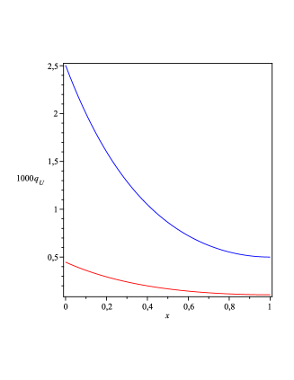
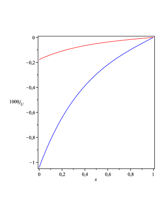
Figure 1: The fluid fluxes from blood to tissue $q_{U}$ (in $min^{-1}$) and across tissue $j_{U}$ (in $min^{-1}\cdot cm$ ) as a function of distance from peritoneal cavity $x$ (in $cm$) for $\nu=(\nu_{max}+\nu_{min})/2$, $\sigma_{TG}=0.001$ (red curve), $\sigma_{TG}=0.01$ (blue curve), and $\sigma_{TA}=0.0$.

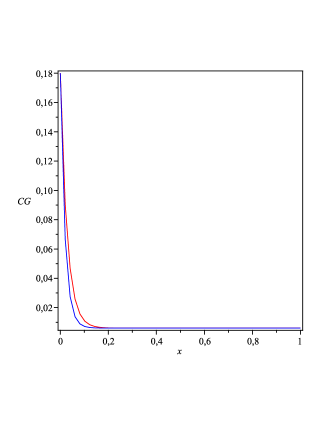
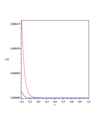
Figure 2: The profiles of glucose concentration in the tissue $C_{G}$ (in $mmol\cdot mL^{-1}$) as a function of distance from the peritoneal cavity $x$ (in $cm$) for $\nu=(\nu_{max}+\nu_{min})/2$, $\sigma_{TG}=0.001$ (red curve) and $\sigma_{TG}=0.01$ (blue curve). Left panel for $0\leq x\leq 1$, right panel: zoom for $0.2\leq x\leq 1$.

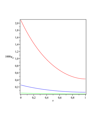
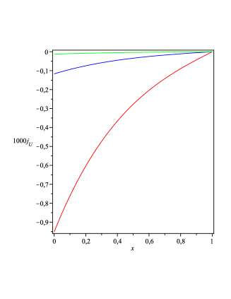
Figure 3: The fluid flux from blood to tissue $q_{U}$ (in $min^{-1}$) and the fluid flux across tissue $j_{U}$ (in $min^{-1}\cdot cm$ ) as a function of distance from the peritoneal cavity $x$ (in $cm$) for $\nu=\nu_{max}-(\nu_{max}-\nu_{min})x$, $\sigma_{TA}=0.5$, and $\sigma_{TG}=0.001$ (green); $0.002$ (blue); $0.01$ (red).

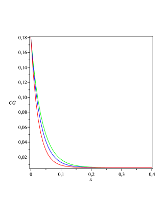
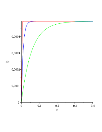
Figure 4: The glucose concentration profiles, $C_{G}$ (in $mmol\cdot mL^{-1}$), and albumin concentration profiles, $C_{A}$ (in $mmol\cdot mL^{-1}$) , in the tissue as a function of distance from the peritoneal cavity, $x$ (in $cm$), for $\nu=\nu_{max}-(\nu_{max}-\nu_{min})x$, $\sigma_{TA}=0.5$, and $\sigma_{TG}=0.001$ (green); $0.002$ (blue); $0.01$ (red).

Using the value of the fluid flux $j_{U}$ at the point $x=0$, one may again calculate the ultrafiltration flow to the peritoneal cavity that can be obtained under the assumed here restrictions on the model parameters. In the case $\sigma_{TG}=0.01$ the total fluid outflow from the tissue to the cavity is approximately equal to $4.8$ $mL/min$, while it is very small ($0.06$ $mL/min$) for $\sigma_{TG}=0.001$. To obtain the values of the ultrafiltration corresponding to those measured during peritoneal dialysis, we need to set $\sigma_{TG}\geq 0.02$. For example, setting $\sigma_{TG}=0.02$ and $\sigma_{TG}=0.03,$ we obtain the ultrafiltration $10$ $mL/min$ and $15$ $mL/min$, that are close to those measured in clinical conditions for similar boundary concentration of glucose (Smit et al 2004a, Smit et al 2004b, Waniewski et al 1996a, Waniewski et al 2009, Stachowska et al 2012). The initial values of ultrafiltration remain in agreement with values obtained by our group in clinical studies (Waniewski et al 1996b; Waniewski 2007). The initial rates of ultrafiltration for 3.86% glucose solution were found to be of $15$ $mL/min$, which was much higher than those for 2.27 and 1.36% glucose solutions, 8 and 6 ml/min, respectively (Waniewski et al 1996a,Waniewski et al 1996b). Similar values in the range of $14-18$ $mL/min$ were measured during the initial minute and much lower values of $4-8$ $mL/min$ at the end of a 4-h dwell study with 3.86% glucose solution (Smit et al. 2004a; Smit et al. 2004b).

The spatial distributions of the glucose and albumin concentrations for different values of $\sigma_{TG}$ are pictured in Fig. 4. Note that glucose concentration in the tissue, $C_{G}$, again decreases rapidly with the distance from the peritoneal cavity to the constant steady-state $C^{*}_{G}$ in the deeper tissue layer. The glucose concentration is practically equal to $C^{*}_{G}$ for any $x>0.1$ $cm$ if $\sigma_{TG}$ is large ($\geq 0.01$). The tissue layer with non-constant $C_{G}$ is slightly wider if $\sigma_{TG}$ is small ($\leq 0.002$). For such values of $\sigma_{TG}$, the glucose concentration is equal to $C^{*}_{G}$ for any $x>0.2$ $cm.$

The albumin concentration in the tissue, $C_{A}$, is decreased ( in the direction to the peritoneal cavity) in a thin layer, whereas it remains unperturbed in the deeper tissue layers (Fig. 4). This decrease corresponds to the transport of albumin to the peritoneal cavity that is most pronounced close to the peritoneal surface. We found that the albumin concentration essentially depends on the parameter $\sigma_{TG}$. In fact, three curves presented in Fig. 4 show that the tissue layer with decreased $C_{A}$ is wide for $\sigma_{TG}=0.001$, whereas it much smaller for $\sigma_{TG}=0.002$ and almost vanishes for $\sigma_{TG}=0.01$. In the case $\sigma_{TG}=0.001$, the tissue layer of decreased $C_{A}$ is about $0.3$ $cm$ indicating the removal of albumin from this part of the tissue. In the case of high $\sigma_{TG}$, the albumin concentration in the tissue is decreased only in a very thin layer, while it remains at physiological level and equal to $C^{*}_{A}$ (see formula (15)) behind this layer. Thus, high ultrafiltration flow contributes to the fast inflow of albumin from blood to the tissue and drags albumin from deep to subsurface layers. However, the diffusive leak of albumin from the tissue to the peritoneal cavity is faster with high ultrafiltration because of higher concentration gradient (Fig. 4).

5. Conclusions

In this paper, a new mathematical model for fluid transport in peritoneal dialysis was constructed. The model is based on a three-component nonlinear system of two-dimensional partial differential equations and the relevant boundary and initial conditions. To analyze the non-uniform steady-state solutions, the model was reduced to the non-dimensional form. Under additional assumptions the problem was simplified in order to obtain analytical solutions in an explicit form. As the result, the exact formulae for the density of fluid flux from blood to tissue and the fluid flux across the tissue were constructed together with two linear autonomous ODEs for glucose and albumin concentrations in the tissue.

The analytical results were checked for their applicability to describe the fluid-glucose-albumin transport in peritoneal dialysis. The selected values of the parameters were based on previous experimental and clinical studies or estimated from the data using the distributed model. Some of the parameters (Staverman reflection coefficients) were varied to check their impact on the model predictions. The model presented in the current study was extended, compared to the previous studies, by including the transport of water and two most important solutes related to water transport: glucose that is used as osmotic agent and albumin that is the primary determinant of oncotic pressure. These two solutes differ much (300 times) in molecular mass and therefore also differ in their transport parameters. The other studies include mostly only one of these two solutes into the model (Flessner et al. 1984; Baxter and Jain 1989,1990,1991; Cherniha and Waniewski 2005; Flessner 2006; Cherniha et al. 2007; Waniewski et al. 2007,2009; Stachowska-Pietka et al. 2007,2012). On the other hand, our investigations are restricted to the steady state solutions, whereas in real dialysis the fluid and solute transport changes because of the change in boundary conditions (Stachowska-Pietka et al. 2006). We did not included into the model the phenomena of vasodilation and change in tissue hydration that yield spatially non-uniform structure of the tissue (however, our x-dependent fractional volume of interstitial fluid $\nu$ takes into account a part of this non-uniformity of the structure) and contribute to the details of numerical solutions as compared to clinical data (Smit et al 2004a). Only some of the model predictions can be compared directly to clinical data. The most important for us is the rate of ultrafiltration of water to the peritoneal cavity that is induced by glucose. With the concentration of glucose applied in our calculations the ultrafiltration rate of about 15 $mL/min$ is expected (Heimbürger et al. 1992; Waniewski et al. 1996a,1996b; Smit et al 2004a; Smit et al 2004b). Our results demonstrate that this value can be obtained if reflection coefficient for glucose is high (0.02 - 0.03). This general observation is in agreement with the early measurements of these coefficients, but differs from much higher values of the coefficient estimated previously by numerical simulations (Stachowska-Pietka et al. 2006; Waniewski 2007; Waniewski et al. 2007). The difference might be explained by the difference between glucose reflection coefficients for the tissue (low) and the capillary wall (high) obtained from previous numerical simulations, whereas these two coefficients were equal (with a medium value to yield the demanded ultrafiltration rate, for the sake of mathematical tractability) in our predictions (see below).

The glucose and albumin profiles obtained from our model are similar to those found in experimental studies (no such data are available for humans) and to the previous numerical simulations of clinical dialysis (Flessner et al. 2006;Waniewski et al. 2009; Stachowska-Pietka et al. 2012). The glucose interstitial concentration sharply decreases within 2 $mm$ from the peritoneal surface and is equal to its blood concentration in deeper tissue layers, see Figures 2 and 4, as it found previously in other numerical studies (Waniewski et al. 2009; Stachowska-Pietka et al. 2012). A similar profile was found in experiments performed in rats with manitol, which has identical transport characteristics as glucose (Flessner et al. 2006). In contrast, the interstitial concentration of albumin is high within the deep layers of tissue and decreases sharply in a thin layer close to the peritoneal tissue, Figures 2 and 4. This low subperitoneal protein concentration (and therefore also oncotic pressure) was confirmed experimentally (Rosengren et al. 2004) and in numerical simulations (Stachowska-Pietka et al. 2007). Some other results, as the profiles of the flux from blood to tissue $q_{U}$, and the flux across tissue, $j_{U}$ ( see Figures 1 and 3), do not have any experimental counterpart and are rarely presented as the results of numerical studies.

Thus, our model, although aimed at the investigation of its mathematical structure with specific coefficient conditions, yielded also some interesting predictions, in spite of rather simple approximations for the fractional interstitial fluid volume $\nu$ that were applied. Even the simplest approximations of $\nu$ by a constant or a linear function yielded the predictions in agreement with the models based on nonlinear dependence of $\nu$ on interstitial hydrostatic pressure. In fact, the monotonically decreasing (with the distance from the peritoneal surface) function $q_{U}(x)$, describing fluid flux from blood to tissue, and the monotonically increasing function $j_{U}(x)$, describing fluid flux across tissue, are in agreement with the experimental data and previously obtained numerical results. Moreover, we calculated the fluid flux $j_{U}(t,x)$ at $x=0$, which describes the net ultrafiltration flow, i.e., the efficiency of removal of water during peritoneal dialysis, because it is important from practical point of view. The results show that the Staverman reflection coefficient for glucose $\sigma_{TG}$ plays the crucial role for the ultrafiltration. To obtain the values of the ultrafiltration corresponding to experimental data, $10-20$ $mL/min$, measured during peritoneal dialysis, we need to set $\sigma_{TG}\geq 0.02$ in the formulae obtained.

The finding that high ultrafiltration flow rates measured in clinical studies may be obtained with relatively low $\sigma_{G}$ of $0.01-0.03$ and at the same time rather high $\sigma_{TG}=\sigma_{G}$ (which is the assumption necessary to get the presented above analytical solutions) is interesting. In fact, much higher values of $\sigma_{G}$ (about 0.5) and lower values of $\sigma_{TG}$ (about 0.005) were used in (Waniewski et al. 2009, Stachowska-Pietka et al. 2012) to obtain similar flow rates. The new solutions constructed above add new perspective to the unsolved problem of the values of $\sigma_{G}$ (see the detailed discussion in (Waniewski et al. 2009, Stachowska-Pietka et al. 2012)). Thus, these new results are worth to be pursuit further not only because of mathematical interest but also of their potential practical applications.

The difference between the present analytical solutions and the previous simulations is also in the profile fluid void volume being the outcome of the simulations whereas here this profile (approximated due to the linear function) is an input to the equations. Other approximations of the fractional fluid volume $\nu$ may in future result in similar exact formulae. In the particular case, the preliminary calculations show that such exact formulae can be obtained when $\nu$ is a decreasing exponential function. However, the assumption about the equality of the reflection coefficients in the tissue and in the capillary wall, which demonstrates an interesting specific symmetry in the equations, can be too restrictive for practical applications of the derived formulae (Waniewski et al. 2009). Therefore, other approaches to find the analytical solutions of the model need to be looked for.

Acknowledgments.

This work was done within the joint project ”Mathematical modeling transport processes in tissue during peritoneal dialysis” between PAS and NAS of Ukraine.

References

- [1] Bateman H (1974) Higher Transcentental Functions, Vol.2. Moscow: Nauka (In Russian).
- [2] Baxter L T, and Jain R K (1989) Transport of fluid and macromolecules in tumors. I. Role of interstitial pressure and convection. Microvasc Res 37 (1), 77-104.
- [3] Baxter L T, and Jain R K (1990) Transport of fluid and macromolecules in tumors. II. Role of heterogeneous perfusion and lymphatics. Microvasc Res 40 (2), 246-63.
- [4] Baxter L T, and Jain R K (1991) Transport of fluid and macromolecules in tumors. III. Role of binding and metabolism. Microvasc Res 41 (1), 5-23.
- [5] Chagnac A, Herskovitz P, Ori Y, Weinstein T, Hirsh J, Katz M, Gafter U.(2002) Effect of increased dialysate volume on peritoneal surface area among peritoneal dialysis patients. J Am Soc Nephrol. 13(10),2554-9.
- [6] Cherniha R, Dutka V, Stachowska-Pietka J and Waniewski J (2007) Fluid transport in peritoneal dialysis: a mathematical model and numerical solutions. In: Mathematical Modeling of Biological Systems, Vol.I. Ed. by A.Deutsch et al., Birkhaeuser, pp.291-298
- [7] Cherniha R, and Waniewski J (2005) Exact solutions of a mathematical model for fluid transport in peritoneal dialysis. Ukrainian Math. J., 57, 1112–1119
- [8] Cherniha R, and Waniewski J (2011) New mathematical model for fluid-glucose-albumin transport in peritoneal dialysis. Preprint: arXiv:1110.1283 [math.AP]
- [9] Collins J M (1981) Inert gas exchange of subcutaneous and intraperitoneal gas pockets in piglets. Respir Physiol 46 (3), 391-404.
- [10] Czyzewska K, Szary B, Waniewski J. (2000) Transperitoneal transport of glucose in vitro. Artif Organs 24, 857-863.
- [11] Dedrick R L, Flessner M F, Collins J M, and Schultz J S (1982) Is the peritoneum a membrane? ASAIO J 5, 1-8.
- [12] Flessner M F (1994) Osmotic barrier of the parietal peritoneum. Am J Physiol 267, F861-870.
- [13] Flessner M F (2001) Transport of protein in the abdominal wall during intraperitoneal therapy. I. Theoretical approach. Am J Physiol Gastrointest Liver Physiol, 281, G424-437.
- [14] Flessner M F (2006) Peritoneal ultrafiltration: mechanisms and measures. Contrib Nephrol 150, 28-36.
- [15] Flessner M F, Deverkadra R, Smitherman J, Li X, and Credit K (2006) In vivo determination of diffusive transport parameters in a superfused tissue. Am J Physiol Renal Physiol 291, F1096-1103.
- [16] Flessner M F, Dedrick R L, and Schultz J S (1984) A distributed model of peritoneal-plasma transport: theoretical considerations. Am J Physiol 246, R597-607.
- [17] Flessner M F, Fenstermacher J D, Dedrick R L, and Blasberg R G (1985) A distributed model of peritoneal-plasma transport: tissue concentration gradients. Am J Physiol 248, F425-435.
- [18] Gokal R and Nolph K D (1994) The Textbook of Peritoneal Dialysis. Dordrecht: Kluwer.
- [19] Gupta E, Wientjes M G, and Au J L (1995) Penetration kinetics of 2’,3’-dideoxyinosine in dermis is described by the distributed model. Pharm Res 12 (1), 108-12.
- [20] Heimbürger O, Waniewski J, Werynski A, and Lindholm B (1992) A quantitative description of solute and fluid transport during peritoneal dialysis. Kidney Int 41, 1320-1332.
- [21] Imholz A L, Koomen G C, Voorn W J, Struijk D G, Arisz L, and Krediet R T (1998) Day-to-day variability of fluid and solute transport in upright and recumbent positions during CAPD. Nephrol. Dial. Transplant., 13 (1), 146-153.
- [22] Katchalsky A, and Curran P F (1965) Nonequilibrium Thermodynamics in Biophysics, Harvard University Press, Cambridge.
- [23] Landis E M, and Pappenheimer J R (1963) Exchange of Substances Through the Capillary Walls. Handbook of Physiology. Circulation. Washington, DC: Am. Physiol. Soc.
- [24] Parikova A, Smit W, Struijk D G, and Krediet, R T (2006) Analysis of fluid transport pathways and their determinants in peritoneal dialysis patients with ultrafiltration failure. Kidney Int 70, 1988-1994.
- [25] Patlak C S, and Fenstermacher J D (1975) Measurements of dog blood-brain transfer constants by ventriculocisternal perfusion. Am J Physiol 229 (4), 877-884.
- [26] Perl W (1962) Heat and matter distribution in body tissues and the determination of tissue blood flow by local clearance methods. J Theor Biol 2, 201-235.
- [27] Perl W (1963) An extension of the diffusion equation to include clearance by capillary blood flow. Ann N Y Acad Sci 108, 92-105.
- [28] Piiper J, Canfield R E, and Rahn H (1962) Absorption of various inert gases from subcutaneous gas pockets in rats. J Appl Physiol 17, 268-274.
- [29] Polyanin A D, Zaitsev V F (2003) Handbook of Exact Solutions for Ordinary Differential Equations. Boca Raton (USA): CRC Press Company.
- [30] Rosengren BI, Carlsson O, Venturoli D, al Rayyes O, and Rippe B (2004) Transvascular passage of macromolecules into the peritoneal cavity of normo- and hypothermic rats in vivo: active or passive transport? J Vasc Res 41,123-30
- [31] Seames E L, Moncrief J W, and Popovich R P (1990) A distributed model of fluid and mass transfer in peritoneal dialysis. Am J Physiol 258, R958-972.
- [32] Smit W, Struijk D G, Pannekeet M M, and Krediet R T (2004a) Quantification of free water transport in peritoneal dialysis. Kidney Int 66, 849-854.
- [33] Smit W, van Esch S, Struijk D G, Pannekeet M M, and Krediet R T (2004b) Free water transport in patients starting with peritoneal dialysis: a comparison between diabetic and non diabetic patients. Adv Perit Dial 20, 13-7.
- [34] Stachowska-Pietka J, Waniewski J, Flessner M F, and Lindholm B (2006) Distributed model of peritoneal fluid absorption. Am J Physiol Heart Circ Physiol 291, H1862-1874.
- [35] Stachowska-Pietka J, Waniewski J, Flessner M F, and Lindholm B (2007) A distributed model of bidirectional protein transport during peritoneal fluid absorption. Adv Perit Dial 23, 23-27.
- [36] Stachowska-Pietka J, Waniewski J, Flessner M F, and Lindholm B (2012) Computer simulations of osmotic ultrafiltration and small solute transport in peritoneal dialysis: A spatially distributed approach. Am J Physiol Renal Physiol 302,F1331-1341.
- [37] Van Liew H D (1968) Coupling of diffusion and perfusion in gas exit from subcutaneous pocket in rats. Am J Physiol 214 (5), 1176-1185.
- [38] Waniewski J (2001) Physiological interpretation of solute transport parameters for peritoneal dialysis. J Theor Med 3, 177-190.
- [39] Waniewski J (2002) Distributed modeling of diffusive solute transport in peritoneal dialysis. Ann Biomed Eng 30, 1181-1195.
- [40] Waniewski J (2007) Mean transit time and mean residence time for linear diffusion-convection-reaction transport system. Comput Math Methods Med 8 (1), 37-49.
- [41] Waniewski J, Dutka V, Stachowska-Pietka J, and Cherniha R (2007) Distributed modeling of glucose-induced osmotic flow. Adv Perit Dial 23, 2-6.
- [42] Waniewski J, Heimbürger O, Werynski A, and Lindholm B (1996a) Simple models for fluid transport during peritoneal dialysis. Int J Artif Organs 19 (8), 455-466.
- [43] Waniewski J, Heimbürger O, Werynski A, and Lindholm B (1996b) Osmotic conductance of the peritoneum in CAPD patients with permanent loss of ultrafiltration capacity. Perit Dial Int 16, 488-496.
- [44] Waniewski J, Stachowska-Pietka J, and Flessner MF (2009) Distributed modeling of osmotically driven fluid transport in peritoneal dialysis: theoretical and computational investigations. Am J Physiol Heart Circ Physiol 296, H1960-1968.
- [45] Wientjes M G, Badalament R A, Wang R C, F. Hassan, and Au J L (1993) Penetration of mitomycin C in human bladder. Cancer Res 53 (14), 3314-20.
- [46] Wientjes M G, Dalton J T, Badalament R A, Drago J R, and Au J L (1991) Bladder wall penetration of intravesical mitomycin C in dogs. Cancer Res 51 (16), 4347-4354.
- [47] Zakaria E R, Lofthouse J, Flessner M F (1999) In vivo effects of hydrostatic pressure on interstitium of abdominal wall muscle. Am J Physiol 276, H517-529.
- [48] Zakaria E R, Lofthouse J, Flessner M F (2000) Effect of intraperitoneal pressures on tissue water of the abdominal muscle. Am J Physiol Renal Physiol 278, F875-885.