Sausage Mode Propagation in a Thick Magnetic Flux Tube

A. Pardi, I. Ballai, A. Marcu, B. Orza

Abstract

The aim of this paper is to model the propagation of slow magnetohydrodynamic (MHD) sausage waves in a thick expanding magnetic flux tube in the context of the quiescent (VAL C) solar atmosphere. The propagation of these waves is found to be described by the Klein-Gordon equation. Using the governing MHD equations and the VAL C atmosphere model we study the variation of the cut-off frequency along and across the magnetic tube guiding the waves. Due to the radial variation of the cut-off frequency the flux tubes act as low frequency filters for waves.

Keywords: Magnetohydrodynamics (MHD), Sun, Waves

Introduction

The dynamical response of the plasma in the solar atmosphere to rapid changes in the solar interior can be manifested through waves propagating within the solar atmosphere. The dynamics of a large class of waves with wavelengths and periods large compared with the ion Larmor radius ($10^{-4}$ m in the solar photosphere and about 1 m for almost all combinations of coronal parameters) and the gyroperiod ($10^{-7}$ s in the solar photosphere and of the order of $10^{-3}$ s in the solar corona), respectively, can be described within the framework of collisional magnetohydrodynamics. Waves perturb macro-parameters of the plasma, such as density, temperature, bulk velocity and magnetic field. The period range of waves and oscillations observed in the solar atmosphere (from a few seconds to a few hundreds of minutes) is well covered by temporal resolution of presently available ground-based and spaceborne observational telescopes. The study of waves and oscillations in the context of solar atmospheric physics has a long history that started more than six decades ago. While until very recently this study was driven mainly by scientific interest, the continuous development and refinement of this important branch of solar and space physics was motivated by the tremendous amount of observations showing the propagation characteristics of waves and oscillations in various solar structures. Nowadays almost all waves labelled as magnetohydrodynamic waves and oscillations are observed with great accuracy. In this context slow MHD waves were observed in the solar photosphere (Zirin72, Dorotovic08, Fujimura09), in the solar chromosphere e.g. Gilbert04, solar corona e.g. Schrijver1999, Nightingale99a, Nightingale99b, Berghmans99, De Moortel00, McEwan06, Berghmans01, Erd08, Marsh09 and solar plumes e.g. DeForest98, Ofman2000. Although initially their observations was not easy (due to their very short period), several evidences were adduced to prove the existence of fast waves e.g. Asai01, Williams01, Williams02, Katsiyannis03, Dorotovic12, in different magnetic structures. A special note should be made regarding the large number of fast kink oscillations of coronal loops observed recently e.g. Aschwanden99, Wang03, Ofman2008, Ballai2011 that served as key ingredient in the development of coronal seismology.

Until recently wave propagation in magnetic guides were modelled especially in the thin flux tube limit (for a review see, e.g. Roberts2001, supposing that the wave length of waves is much larger than the radius of the tube (i.e. $kR\ll 1$). This approximation allows modelling the propagation of waves and oscillations in various magnetic structures in a tractable way since the radial dependence of perturbations is factorised out. While this is a viable limit for waves and oscillations in the solar corona and upper part of the chromosphere where wave lengths are comparable to the length of loops RaeRoberts1982, in the solar photosphere this condition is hardly satisfied. Here, the thin flux tube approximation can be applied to only very thin magnetic structures often found at the edges of granules. In general the structure of the waveguide for waves propagating in the solar photosphere the tube can be considered thick. It is well known that under photospheric conditions the density scale height is of the order of a few hundred kilometers, so any wave that has a wavelength equal or larger than this length will experience the effect of gravitational stratification. If we assume that the wavelength is comparable to the scale-height, the condition of applicability of the thin flux tube approximation reduces to $2\pi R/H\ll 1$. Assuming an isothermal atmosphere the exact value of the scale-height can be determined from the VAL-C model (Vernazza1981). This criterion will be addressed later in our investigation.

In our study we investigate the propagation of waves in magnetic structures that ascend from the convective zone, open up as they reach the chromosphere and then either continue in the corona as opened magnetic flux tubes (Fedun2011) or become horizontal and eventually descend, forming the magnetic canopy.

Magnetic structures channel the propagation (among other various types of waves) of slow longitudinal acoustic waves (for a detailed review see e.g. Roberts2006), and the propagation of these waves in the presence of gravity in the thin flux tube approximation is described by the Klein-Gordon equation (see also Ballai2006, Erdi108). The solution of the Klein-Gordon equation in this case describes the behaviour of slow MHD waves propagating with a phase speed close to the tube speed and the propagation of a wake following the wave that propagates with the cut-off frequency. The cut-off frequency in this context is defined as a threshold limit of frequencies and represents the lower value of frequencies describing the propagating waves. In the opposite case, when the frequencies of waves are smaller than the cut-off frequency, waves will become evanescent, i.e. eigenfunctions will fall-off exponentially with distance. Observations show (since 1964) (Aschwanden2006) that the cut-off frequencies for these longitudinal axi-symmetric displacements vary on average between 0.025 and 0.03 Hz.

The paper is organised as follows: in Section 2 we will describe the thick expanding magnetic flux tube model (and obtain the equations of the magnetic field) and we will determine the evolutionary equation of slow sausage waves propagating in structures of this type. Using simple mathematical methods and straightforward assumptions we will reduce the evolutionary equation to a Klein-Gordon type equation and we will determine the expression of the cut-off frequency for thick magnetic tubes in Section 3. In Section 4 the formulaic expression will be joined with a realistic atmospheric model that will help us study the evolution of the cut-off frequency in longitudinal and transversal direction of the tube. Finally our results will be summarised and conclusions will be drawn in Section 5.

The mathematical and physical considerations of the problem

We consider a gravitationally structured elastic magnetic flux tube that at the height $z=0$ has a radius $R_{0}$ and a cross section $A_{0}$. Due to decrease of the equilibrium parameters (density and pressure) with height, the tube is expanding in the horizontal direction. We will consider a 2D equilibrium magnetic field with components $\textbf{B}_{0}=(B_{r},0,B_{z})$, each one of them being both r and z dependent. For simplicity we assume that the equilibrium magnetic field is potential (a special case of force-free fields). As a result, the equations that can fully describe the structure of the magnetic field are

$$\nabla\times{\bf B_{0}}=0,\quad\nabla\cdot{\bf B_{0}}=0,$$ (1)

where the second equation is the solenoidal condition.

Written in cylindrical geometry, the above two equations can be reduced to a PDE for the $z$-component of the magnetic field

$$\frac{1}{r}\frac{\partial B_{z}}{\partial r}+\frac{\partial^{2}B_{z}}{\partial r^{2}}+\frac{\partial^{2}B_{z}}{\partial z^{2}}=0.$$ (2)

Equation (2) can be solved by using the separation of the variables method in which case we write $B_{z}=F_{1}(r)F_{2}(z)$ therefore Eq.(2) becomes

$$\frac{F_{1}^{{}^{\prime}}(r)}{F_{1}(r)r}+\frac{F_{1}(r)^{{}^{\prime\prime}}}{F_{1}(r)}=-\frac{\ddot{F_{2}}(z)}{F_{2}(z)}=\lambda,$$ (3)

where $\lambda$ is a separation constant, the dash and dot represent differentiation with respect to $r$ and $z$, respectively. It can be easily shown that the only physically acceptable case is when $\lambda=-\nu^{2}<0$. In this case the solutions of Eq. (3) become

$$F_{1}(r)=d_{1}J_{0}(\nu r)+d_{2}Y_{0}(\nu r),$$ (4)

$$F_{2}(z)=d_{3}e^{\nu z}+d_{4}e^{-\nu z},$$ (5)

where $J_{0}$ and $Y_{0}$ are zeroth order Bessel functions and the quantities $d_{i}$ ($i=1-4$) are constants that can be determined when considering the suitable boundary conditions.

Our intention is to construct such a magnetic field model which that at $z=0$ and at the centre of the tube has perfectly vertical field lines, i.e. $B_{z}(r=0,z=0)=B_{0},B_{r}(r=0,z=0)=0$. As we go higher up in height and further away from the axis, the field lines become more and more tilted with respect to the vertical direction and eventually they become horizontal far away from the vertical symmetry axis. Since the function $Y_{0}(\nu r)$ is divergent at $r=0$ we will choose $d_{2}\equiv 0$, so the radial component reduces to $F_{1}(r)=d_{1}J_{0}(\nu r)$. In addition since observations show that the cross-section of the tube becomes wider (in virtue of the equation of flux conservation) with height we expect that the $z$-component of the magnetic field has to decrease with height, so we consider $d_{3}\equiv 0$. As a result the $z$-component of the magnetic field reduces to

$$B_{z}=d_{1}J_{0}(\nu r)\cdot d_{4}e^{-\nu z}=d_{5}e^{-\nu z}J_{0}\left(\nu r\right)=B_{0}e^{-\nu z}J_{0}\left(\nu r\right),$$ (6)

where $B_{0}$ is the field strength at $r=z=0$.

Using the solenoidal condition, it is easy to show that the radial component of the magnetic field can be written as

$$B_{r}=B_{0}e^{-\nu z}J_{1}(\nu r).$$ (7)

The particular form of the $z$-component of the magnetic field is essential for determining the variation of the radius of the tube with height. Assuming that the magnetic flux in the normal direction to the cross-section of the tube is conserved (i.e. ${\bf A}\cdot{\bf B}=const$, where ${\bf A}=A{\bf n}$ with ${\bf n}$ the unit vector perpendicular to the cross-section of the tube pointing upward) it is easy to show that the variation of the radius of the tube is described by

$$R(z)=R(0)e^{\nu z/2}\left[\frac{J_{0}(\nu R(0))}{J_{0}(\nu R(z))}\right]^{1/2},$$ (8)

where $R(0)$ is the radius of the tube at $z=0$. The above transcendental equation is solved numerically using the Newton-Raphson method. The variation of the magnetic fields lines are shown in Figure 1.

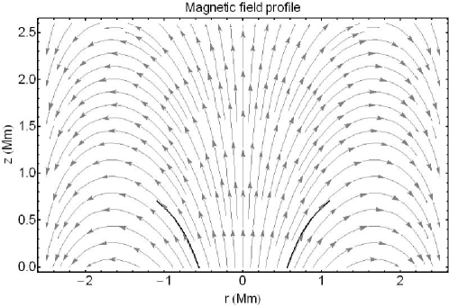
Figure 1: Representation of the magnetic field lines and the flux tube whose boundary is calculated with the help of Eq. (8). The longitudinal axis of the tube is situated at $R=0$.

The magnetic field lines diverge as initially assumed and the inclination of the field lines become larger with the distance from the axis of the tube. The axis of the flux tube is situated at $R=0$ and the radius of the tube at $z=0$ is chosen to be 560 km while at the height of 750 km the radius becomes 1160 km. The value of $\nu$ is arbitrary and its value $1.44\times 10^{-6}$ was chosen in such a way to ensure that the decay of the magnetic field with height is realistic. In this way, the magnetic field at $z=0$ and $r=0$ is 250 G while at the height of 750 km this becomes 85 G.

With the help of the tube’s radius and the scale-height determined from the VAL-C model, we can finally justify our choice of thick flux tube in the solar photosphere (see Fig 2). As we specified earlier, a magnetic flux tube is thin provided $2\pi R/H\ll 1$. Combining our findings for the radius and a realistic atmospheric model it is obvious that the criterion for a thin flux tube is not satisfied for the whole height range we considered.

Figure 2: The variation of $2\pi R/H$ in the solar photosphere. According to the standard criterion, a flux tube is classified as thin if this quantity is much less than one.

Now that the magnetic structure of the model is established we can study the dynamics of waves. Small amplitude disturbances of the equilibrium state of the gravitationally stratified atmosphere inside the tube can be described by the linear MHD equations in cylindrical coordinates

$$\frac{\partial\rho^{{}^{\prime}}}{\partial t}A+\rho\frac{\partial A^{{}^{\prime}}}{\partial t}+\nabla\cdot\left(\rho A\textbf{v}\right)=0,$$ (9)

$$\rho\frac{\partial\textbf{v}}{\partial t}=-\nabla p^{{}^{\prime}}+\frac{1}{\mu}\left[\left(\nabla\times\textbf{B}^{{}^{\prime}}\right)\times\textbf{B}_{0}\right]+\textbf{g}\rho^{{}^{\prime}},$$ (10)

$$\frac{\partial p^{{}^{\prime}}}{\partial t}+\gamma p\left(\nabla\cdot\textbf{v}\right)+\left(\textbf{v}\cdot\nabla\right)p=0,$$ (11)

$$\nabla\cdot\textbf{B}^{{}^{\prime}}=0.$$ (12)

In the above equations, $p(z)$, $\rho(z)$, $\textbf{B}_{0}=(B_{r},0,B_{z})$, $A(z)$ denote the equilibrium pressure, density, magnetic field, cross-section area of the tube. The dashed quantities represent perturbations, $\textbf{v}=(v_{r},0,v_{z})$ is the velocity perturbation, $\mu$ is the magnetic permeability of free space, g is the gravitational acceleration and $\gamma$ is the adiabatic index (from now one the dash will always denote a perturbation).

The above equations will be supplemented by the transverse pressure balance condition that must be satisfied at every height of the tube

$$p^{{}^{\prime}}+\frac{B_{0}\cdot B^{{}^{\prime}}}{2\mu}=P_{e},$$ (13)

where $P_{e}$ is the total pressure in the exterior environment (includes kinetic and magnetic contributions but it’s exact form is not important for the present analysis). In addition, we require that the magnetic flux along the tube is constant, so

$$A(z)B^{{}^{\prime}}_{z}+A^{{}^{\prime}}(z)B_{z}=ct.$$ (14)

The evolutionary equation for slow MHD waves in thick flux tubes

This section is devoted to the determination of the evolutionary equation describing the propagation of slow sausage waves in thick flux tubes under photospheric conditions. In order to obtain a physically acceptable equation some assumptions will be made regarding the direction of the dominant dynamics.

Using Eq. (9), (11), (12), (13), (14) and the radial and longitudinal components of the momentum equation (10), it is rather straightforward to show that these equations can be reduced to

$$\frac{\partial^{2}v_{r}}{\partial t^{2}}=c_{0}^{2}\left(\frac{1}{r}\frac{\partial v_{r}}{\partial r}-\frac{v_{r}}{r^{2}}+\frac{\partial^{2}v_{r}}{\partial r^{2}}\right)+\frac{\tau}{\rho}\frac{\partial p}{\partial z}+\frac{B_{z}}{\mu\rho}\left(\frac{\partial^{2}B^{{}^{\prime}}_{r}}{\partial z\partial t}-\frac{\partial^{2}B^{{}^{\prime}}_{z}}{\partial r\partial t}\right),$$ (15)

and

$$\frac{\partial^{2}v_{z}}{\partial t^{2}} = \frac{1}{\rho}\frac{\partial}{\partial z}\left[\gamma p\left(\frac{v_{r}}{r}+\frac{\partial v_{r}}{\partial r}+\frac{\partial v_{z}}{\partial z}\right)+v_{z}\frac{\partial p}{\partial z}\right]-\frac{B_{r}}{\mu\rho}\left(\frac{\partial^{2}B^{{}^{\prime}}_{r}}{\partial z\partial t}-\frac{\partial^{2}B^{{}^{\prime}}_{z}}{\partial r\partial t}\right)$$ (16)

$${}+g\left[\frac{1}{A\rho}\nabla\cdot\left(\rho A\textbf{v}\right)-\frac{1}{B_{z}}\frac{\partial B^{{}^{\prime}}_{z}}{\partial t}\right],$$

where we assumed that the variation of $v_{z}$ with respect to the coordinate $r$ is constant and we write $\frac{\partial v_{z}}{\partial r}=\tau$. In the above equations $c_{0}$ is the sound speed defined as $c_{0}(z)=\sqrt{{\gamma p(z)}/{\rho(z)}}$.

Equation (11) and (13) can be combined into

$$\frac{\partial B^{{}^{\prime}}_{r}}{\partial t}=\left[\frac{\partial P_{e}}{\partial t}+\gamma p\left(\nabla\cdot\textbf{v}\right)+v_{z}\frac{\partial p}{\partial z}-\frac{\partial B^{{}^{\prime}}_{z}}{\partial t}\right]\frac{\mu}{B_{r}}.$$ (17)

In a strong magnetic field slow waves propagate predominantly along the field and especially in magnetic flux tubes the slow mode is strongly wave guided along the tube. In his study Roberts (2006) found a simple method for extracting information about slow modes from the MHD equations without the need to calculate the behaviour of all the MHD modes, introducing a spatial and temporal scaling of the form

$$r=\epsilon R,z=Z,t=T,$$ (18)

$$v_{r}=\epsilon u_{r},v_{z}=u_{z},B^{{}^{\prime}}_{r}=\epsilon b^{{}^{\prime}}_{r},B^{{}^{\prime}}_{z}=b^{{}^{\prime}}_{z}.$$ (19)

For $\epsilon\ll 1$ the transverse components and derivatives are much larger than the longitudinal ones, so the slow mode related terms can be depicted as the ones containing the lowest order of $\epsilon$. Using this scaling we ensure that the dynamics of slow waves can be derived without the need of treating other waves and that the dominant dynamics of the plasma is corresponding to slow MHD waves.

Applying the above scaling to Eq. (17) and collecting terms of the same order of $\epsilon$ we obtain (after returning to the initial notation)

$$\frac{B_{r}}{\mu}\frac{\partial B^{{}^{\prime}}_{r}}{\partial t}=\frac{\partial P_{e}}{\partial t},$$ (20)

and

$$\frac{B_{z}}{\mu}\frac{\partial B^{{}^{\prime}}_{z}}{\partial t}=\gamma p\left(\nabla\cdot\textbf{v}\right)+v_{z}\frac{\partial p}{\partial z}.$$ (21)

Applying the same scaling to Eg.(15) we obtain

$$\frac{\partial v_{r}}{\partial t}=\frac{B_{z}}{\mu B^{2}_{r}}\left(\frac{\partial P_{e}}{\partial z}B_{r}-\frac{\partial B_{r}}{\partial z}P_{e}\right).$$ (22)

Finally, using Eqs. (16), (20) and (21) one can derive the expression

$$\frac{\partial^{2}v_{z}}{\partial t^{2}}-c_{o}^{2}\frac{\partial^{2}v_{z}}{\partial z^{2}}-\frac{\partial v_{z}}{\partial z}\left(\frac{1}{\rho}\frac{\partial p}{\partial z}+\Gamma\right)-v_{z}\Lambda=c^{2}_{0}\frac{\partial\Xi}{\partial z},$$ (23)

where we introduced the notations

$$\Gamma=\frac{\gamma}{\rho}\frac{\partial p}{\partial z}+g-\frac{c^{2}_{0}}{v^{2}_{Az}}g,\quad v^{2}_{Az}=\frac{B_{z}^{2}}{\mu\rho},$$ (24)

$$\Lambda=\frac{1}{\rho}\frac{\partial^{2}p}{\partial z^{2}}+\frac{g}{A}\frac{\partial A}{\partial z}+\frac{g}{\rho}\frac{\partial\rho}{\partial z}-\frac{g}{\rho}\frac{\partial p}{\partial z}\frac{1}{v^{2}_{Az}},$$ (25)

$$\Xi=\frac{1}{r}\frac{\partial}{\partial r}\left[\frac{rB_{z}}{\mu B_{r}^{2}}\left(\frac{\partial P_{e}}{\partial z}B_{r}-\frac{\partial B_{r}}{\partial z}P_{e}\right)\right].$$ (26)

Equation (23) is a partial differential equation describing the evolution of the slow wave variable, $v_{z}$, in space and time while the term on the right hand side depends solely on external pressure and the values of the equilibrium magnetic field.

Assuming a solution of the form $v_{z}=Qe^{\lambda(z)z}=Qe^{c(z)}$ and after dividing Eq. (23) by $e^{c(z)}$, we arrive at

$$\frac{\partial^{2}Q}{\partial t^{2}}-c_{0}^{2}\frac{\partial^{2}Q}{\partial z^{2}}-\frac{\partial Q}{\partial z}\left(c^{2}_{o}2C+\frac{1}{\rho}\frac{\partial p}{\partial z}+\Gamma\right)$$ (27)

$$-Q\left[c_{0}^{2}\left(C^{2}+C^{{}^{\prime}}\right)+\left(\frac{1}{\rho}\frac{\partial p}{\partial z}+\Gamma\right)C+\Lambda\right]=c_{0}^{2}\frac{\partial\Xi}{\partial z}\cdot e^{-c(z)},$$

where

$$C(z)=\frac{dc(z)}{dz},C(z)^{{}^{\prime}}=\frac{dC(z)}{dz}.$$ (28)

Next, we are going to choose the function $C(z)$ so that the coefficient of ${\partial Q}/{\partial z}$ vanishes. As a result, we obtain that the dynamics of the slow sausage waves in thick flux tubes is given by a Klein-Gordon equation

$$\frac{\partial^{2}Q}{\partial t^{2}}-c_{0}^{2}\frac{\partial^{2}Q}{\partial z^{2}}+Q\omega_{c}^{2}=c_{0}^{2}\frac{\partial\Xi}{\partial z}e^{-c(z)},$$ (29)

where the term multiplying Q is the cut-off frequency and its expression is given by

$$\omega_{c}^{2}=\frac{1}{4c_{0}^{2}}\left(\frac{1}{\rho}\frac{\partial p}{\partial z}+\Gamma\right)^{2}+c^{2}_{0}\frac{\partial}{\partial z}\left(\frac{\frac{1}{\rho}\frac{\partial p}{\partial z}+\Gamma}{2c^{2}_{0}}\right)-\Lambda.$$ (30)

The cut-off frequency has a complex form and it contains all the main plasma parameters, being dependent on pressure, density, cross section of the tube and their variation with height, as well as the on the plasma beta parameter and the chosen profile of the magnetic field. Eq. (29) shows that slow waves will propagate with the internal sound speed in accordance with the dispersion diagram determined by Edwin83 for photospheric conditions. This is contrast to the findings of wave propagation in thin flux tubes, where the propagation speed is the tube speed. Since at this stage we are not interested in the eigenfunction of Eq. (29) we will not solve this equation, instead we concentrate on the variation of the coefficient given by Eq. (30) with height and radial distance.

In principle the radial component of the magnetic field would considerably modify the value of the Brunt-$V\ddot{a}is\ddot{a}l\ddot{a}$ buoyancy frequency but since our magnetic field was assumed force-free, the magnetic contribution to this important quantity vanishes and its value is given by the classical formula.

Results and Discussions

Having determined the analytical form of the cut-off frequency (see Eq. (30)), we are now interested in its profile inside the expanding tube and its variation with height and radial distance. In order to obtain actual values for this important physical parameter we consider the observational data provided by the VAL III C model Vernazza1981 for the quiet sun (consider that no extreme magnetic phenomena are taking place in the proximity of the flux tube) because of its simplicity.

The magnetic field profile derived earlier allows us to find the value of its components in every point inside the tube. The value of the magnetic field is important for the present analysis as this will control the evolution of other physical parameters through the total pressure balance. The VAL III C model data provided us with values for pressure, density, and temperature at certain heights. We assume that the pressure extracted from the atmospheric model represents the kinetic pressure in the external region. We consider that the tube is embedded in a quiescent environment, the magnetic field strength at the footpoint inside the tube was taken to be 250 G. Because of the poor fit of the magnetic field profile with the observational data, we were constrained to consider additionally a very weak magnetic field in the surrounding environment (60 G). Since the exact value of the magnetic field profile of the tube can be determined with the help of Eqs. (6)-(7) we can derive the equilibrium pressure in the interior of the tube at different heights. For simplicity we assumed that in the radial direction the magnetic flux tube is isothermal resulting in an equilibrium pressure that depends only on height. Once the equilibrium pressure was determined, the hydrostatic pressure balance was used to determine the profile of the density inside the tube. With the help of these values, the determination of characteristic speeds (sound speed and Alfvén speed) was straightforward. These speeds can help us determining the plasma-beta ($\beta$) inside the tube. Through the Alfvén speed, the plasma-beta will depend not only on height but also on radial direction. The variation of $\beta$ for two different radial distances is plotted in Fig. (3) where $R_{max0}$ represents the maximum radius of the tube determined by means of Eq. (8) and a second level at which the plasma-beta is calculated was taken at $R_{0}=50km$ from the axis of the tube. The distance of this reference level from the axis of the tube is also changing with height.

Figure 3: The variation of plasma-beta with height for two values of he radial distance from the longitudinal axis of the tube (at $r=0$).

It is obvious that the value of $\beta$ decays with height and for a given height it becomes smaller closer to the axis of the tube. The results are in concordance with the recent realistic plasma beta profiles (ssFedunVerth2011) for heights above 500 km. This difference it is likely to be due to the force field assumption that we have chosen for our theoretical model.

Now that all physical quantities entering the expression of the cut-off frequency are determined, we can plot the dependence of the cut-off frequency on the two directions (see Fig.4).

Figure 4: Cut-off frequency profile (height and radial dependence) inside the tube (up to 605 km in height).

In Fig.4 we plot the obtained values for the cut-off frequency with respect to the position along the tube radius for various heights. The values of the cut-off frequency are decreasing with height, meaning that waves can propagate easier if the driver of the disturbance is situated above the foot point, inside the loop, and if the waves are propagating closer to the axis rather than closer to the tube’s boundary. Due to the radial dependence of the cut-off frequency, we can conclude that the region near the axis of the tube allows a wider range of wave frequencies to propagate upwards that the region near the boundary. Our results show that a magnetic flux tube acts as a frequency filter for upward propagating waves.

Figure 5: Cut-off frequency profile(height and radial dependence) inside the tube (from 450km to 705km in height)

A ”blown-up” section of Fig. 4 for small values of the cut-off frequency is shown in Fig. 5 and the pattern of the variation of this frequency with height and radial dependence is maintained.

The 3D dependence of the cut-off frequency with the two coordinates can be seen in Fig 6 where the edge of the tube can be seen as the point in the ($r-z$) plane where the cut-off frequency drops to zero.

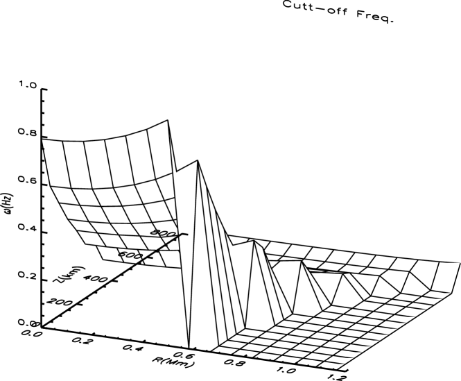
Figure 6: The variation of the cut-off frequency with height and radial distance from the axis of the flux tube.

The recovered cut-off frequencies are somehow larger than the expected values, especially for lower heights. Although our intention was to show how a magnetic flux tube can act as a frequency filter for slow sausage waves propagating in the lower photosphere, the recovered frequencies are not in line with the expected values indicating that some important physical effect(s) was neglected. One possibility that can reduce the value of the cut-off frequency is the inclusion of dissipative effects. In an earlier paper Ballai2006 studied the propagation of slow MHD waves in a stratified and viscous plasma and they found that the evolutionary equation of these waves was described by the Klein-Gordon-Burgers equation where the cut-off frequency was reduced by a term proportional to the square of the coefficient of viscosity. It is possible that if realistic transport mechanisms are taken into account (including ambipolar diffusion due to the partial ionisation of photospheric plasma) the true value of the cut-off frequency can be reduced to an acceptable level. Another important factor that could influence the value of the cut-off frequency is the consideration of a filed-aligned equilibrium flow, something that has been observed in the solar photosphere. Finally, discrepancies in the value of the cut-off frequency can appear due to the simplistic model our paper used. An improved model where all restrictions imposed in our paper are relaxed would require a fully numerical investigation.

Conclusion

In this study we investigated the variation of the cut-off frequency imposed by the plasma in the case of propagation of slow sausage waves in thick flux tubes in the solar atmosphere. The prescribed magnetic field is force-free. The particular choice of the magnetic filed allowed us to derive an evolutionary equation of waves in the form of a Klein-Gordon equation. Apart from describing the dynamics of slow waves, this equation also gives the value of the cut-off frequency, i.e. the lower limit of frequencies at which waves can still propagate through the magnetic and stratified plasma. The total pressure balance equation satisfied at every height of the tube was used to connect the values of the VAL III C model atmospheric model with the plasma inside the flux tube.

Our intention was not to solve the evolutionary equation; given the built-up of our model, this task would require an extensive numerical analysis. Instead we focussed our attention to one of the coefficients of the evolutionary equation that represents the cut-off frequency. Our derived values for the cut-off frequency show that the tube acts as a frequency filter, the cut-off values depending on the radial distance and height. The recovered values are somehow larger than the expected, especially at lower heights but this could be attributed to either the simplistic model employed by our study or to some essential physics that was neglected.

1 Acknowledgements

The present study was completed while one of us (AP) visited the Solar Physics and Space Plasma Research Centre (SP2RC) at the University of Sheffield. IB was financially supported by NFS Hungary (OTKA, K83133).

References

Asai01: Asai, A. et al.: 2001, Periodic acceleration of elecrons in the 1998 November 10 solar flare, ApJ, 562, L103-L106.

Aschwanden99: Aschwanden, M.J., Fletcher, L., Schrijver, C.J. and Alexander, D.: 1999, Coronal loop oscillations observed with the Transition Region and Coronal Explorer, ApJ, 520, 880-894.

Aschwanden2006: Aschwanden, M.J.: 2006, Physics of the Solar Corona, Printer and Praxis Publishing, Chichester, UK.

Ballai2006: Ballai, I., Erdélyi, R. and Hargreaves, J: 2006, Slow magnetohydrodynamic waves in stratified and viscous plasmas, Phys.Plasmas, 13.

Ballai2011: Ballai, I., Jess, D.B. and Douglas, M.: 2011, TRACE observations of the driven loop oscillations, AAp, 534.

Berghmans99: Berghmans, D., Clette, F.: 1999, Active region EUV transient brightenings- First Results by EIT of SOHO JOP 80, SolPhys, 186, 207-229.

Berghmans01: Berghmans, D., McKenzie, D. and Clette, F.: 1999, Active region transient brightenings. A aimultaneous view by SXT, EIT and TRACE, AAp, 369, 291-304.

DeForest98: DeForest, C.E. and Gurman, J.B.: 1998, Observation of quasi-periodic compressive waves in solar polar plumes, ApJ, 501, L217-L220.

De Moortel00: De Moortel, I. and Hood, A.W.: 2000, Wavelet analysis and the determination of coronal plasma properties, AAp, 363, 269-278.

Dorotovic08: Dorotovic, I., Erdélyi, R. and Karlovsky, V.: 2008, IAU Symp.(ed), Identification of linear slow sausage waves in magnetic pores, 247.

Dorotovic12: Dorotovic, I., Erdélyi, R., Freij, N., Karlovsky, V., Marquez, I.: 2012, On standing sausage waves in photospheric magnetic waveguides, AAp, 1210.

Edwin83: Edwin, P.M. and Roberts, B.: 1983, Wave propagation in a magnetic cylinder, SolPhys, 99.

Erd108: Erdélyi, R. and Hargreaves, J.: 2008, Wave propagation in steady stratified one-dimentional cylindrical waveguides, AAp, 483, 285-295.

Erd08: Erdélyi, R. and Taroyan, Y.: 2008, Hinode EUV spectroscopic observations of coronal oscillations, AAp, 489, L49-L52.

Fedun2011: Fedun, V. et al.: 2011, Numerical Modeling of Footpoint-Driven Magneto-Acoustic Wave Propagation in a Localized Solar Flux Tube, ApJ, 727, 17-31.

FedunVerth2011: Fedun, V., Verth, G., Jess, D.B., and Erdélyi, R.: 2011, Frequency filtering of torsional Alfven waves by chromospheric magnetic filed, ApJ, 740.

Fujimura09: Fujimura, D. and Tsuneta, S.: 2009, Properties of magnetohydrodynamic waves in the solar photosphere obtained with HINODE, ApJ, 702, 1443-1457.

Gilbert04: Gilbert, H.R. and Holzer, T.E.: 2004, Chromospheric waves observed in the He I spectral line ($\lambda=10830\AA$): a closer look, ApJ, 610, 572-587.

Katsiyannis03: Katsiyannis, A.C., Williams, D.R., McAteer, R.T.J., Gallagher, P.T., Keenan, F.P., Murtagh, F.: 2003, Eclipsa observations of high-frequency oscillations in active region coronal loops, AAp, 406, 709-714.

Marsh09: Marsh, M.S., Walsh R.W. and Plunkett, S.: 2009, Three-dimensional coronal slow modes: towards three-dimensional seismology, ApJ, 697, 1674-1680.

McEwan06: McEwan, M.P. and De Moortel, I.: 2006, Longitudinal intensity oscillations observed with TRACE: evidence of fine-scale structure, AAp, 448, 763-770.

Nightingale99a: Nightingale, R.W., Aschwanden, M.J., Hurlburt, N.E.: 1999, Time Variability of EUV Brightning in Coronal Loops Observed with TRACE, SolPhys, 190, 249-265.

Nightingale99b: Nightingale, R.W., Aschwanden, M.J., Hurlburt, N.E.: 1999, Time Variability of Coronal Loops observed by TRACE, American Astron. Society, 31, 961.

Ofman2000: Ofman, L.: 2000, ASP Series (ed.)Propagation and Dissipation of Slow Magnetosonic Waves in Coronal Plumes, University of Chicago Press (USA), 205.

Ofman2008: Ofman, L. and Wang, T.J.: 2008, Hinode observations of transversal waves with flows in coronal loops, AAp, 482, L9-L12.

RaeRoberts1982: Rae, I.C., Roberts, B.: 1982, Pulse Propagation in a Magnetic Flux Tube, ApJ, 256, 761-767.

Roberts2001: Roberts, B.: 2001, entry Solar Photospheric Magnetic Flux Tubes: Theory, Encyclopedia of Astronomy and Astrophysics, eds Paul Murdin, Nature Publishing Group.

Roberts2006: Roberts, B.: 2006, Slow magnetohydrodynamic waves in the solar atmosphere, Philos. Trans. R. Soc. London, 634, 447-460.

Schrijver1999: Schrijver, C.J., Hurlburt, N.E., Engvold, O., Harvey, J.W.: 1999, Physics of the solar corona and the transition region. Part 1,2. Proceedings. Workshop, Monterey, CA (USA), SolPhys, 190, 193, 1-497, 1-297.

Vernazza1981: Vernazza, J.E., Avrett, E.H., Loeser, R.: 1981, Structure of the Solar Chromosphere III. Models of the EUV Brightness Components of the Quiet Sun,ApJ, 45, 635-725.

Wang03: Wang, T.J., Solanski, S.K., Curdt, W., Innes, D.E., Dammasch, I.E., Kliem, B.: 2003, Hot coronal loop oscillations observed with SUMER: Exemples and statistics, AAp, 406, 1105-1121.

Williams01: Williams, D.R. et al.: 2001, High-frequency oscillations in a solar active region coronal loop, mnras, 326, 428-436.

Williams02: Williams, D.R. et al.: 2002, An observational study of a magneto-acoustic wave in the solar corona, mnras, 336, 747-752.

Zirin72: Zirin, H. and Stein, A.: 1981, Observations of running penumbral waves, ApJs, 178, L85-L87.