Interpolating from Bianchi Attractors to Lifshitz and AdS Spacetimes

Abstract:

We construct classes of smooth metrics which interpolate from Bianchi attractor geometries of Types II, III, VI and IX in the IR to Lifshitz or $AdS_{2}\times S^{3}$ geometries in the UV. While we do not obtain these metrics as solutions of Einstein gravity coupled to a simple matter field theory, we show that the matter sector stress-energy required to support these geometries (via the Einstein equations) does satisfy the weak, and therefore also the null, energy condition. Since Lifshitz or $AdS_{2}\times S^{3}$ geometries can in turn be connected to $AdS_{5}$ spacetime, our results show that there is no barrier, at least at the level of the energy conditions, for solutions to arise connecting these Bianchi attractor geometries to $AdS_{5}$ spacetime. The asymptotic $AdS_{5}$ spacetime has no non-normalizable metric deformation turned on, which suggests that furthermore, the Bianchi attractor geometries can be the IR geometries dual to field theories living in flat space, with the breaking of symmetries being either spontaneous or due to sources for other fields. Finally, we show that for a large class of flows which connect two Bianchi attractors, a C-function can be defined which is monotonically decreasing from the UV to the IR as long as the null energy condition is satisfied. However, except for special examples of Bianchi attractors (including AdS space), this function does not attain a finite and non-vanishing constant value at the end points.

1 Introduction

Recent developments suggest that fascinating connections might exist between the study of gravity and condensed matter physics, or more specifically the study of strongly coupled field theories at finite density. See [1, 2, 3, 4] for reviews of this subject with additional references.

On the gravity side, motivated by the varied and beautiful phases found in nature, new brane solutions have been discovered. These branes have new kinds of hair, or have horizons with reduced symmetry. For example, see [5, 6, 7, 8] for discussions on how black hole no-hair theorems can be violated in AdS space in the context of holographic superconductivity; [9, 10, 11] for discussions of how emergent horizons with properties reflecting dynamical scaling in the dual field theory (“Lifshitz solutions”) can arise; and [12, 13, 14, 15, 16, 17, 18] for discussions of horizons exhibiting both dynamical scaling and hyperscaling violation. The earliest work mostly focused on horizons with translational and rotational symmetry, but more recently examples of black brane horizons dual to field theories with further reduced space-time symmetries have been discussed in e.g. [26, 27, 28, 29, 30, 31, 32, 33, 34, 35, 36, 37, 38, 39, 40, 41, 42].

Extremal branes are particularly interesting, since they correspond to ground states of the dual field theory in the presence of a chemical potential or doping. Their near-horizon geometries often exhibit a type of attractor behavior, and as a result, are quite universal and independent of many details. There is a considerable body of work regarding the attractor mechanism, starting with the pioneering work in [43]. A recent review with additional references is [44]. For studies of the attractor mechanism in the non-supersymmetric context, which is the situation of relevance here, see for instance [45, 46, 47, 48, 49, 50].

Of particular interest for this paper are the brane solutions studied in [29, 30], which correspond to phases of matter which are homogeneous but not isotropic. It was shown that in $4+1$ dimensions, such brane solutions can be classified using the Bianchi classification developed earlier for studying homogeneous cosmologies. In [29, 30], it was found that for extremal black branes of this kind, the near-horizon geometry itself often arises as an exact solution for a system consisting of Einstein gravity coupled to (simple) suitable matter in the presence of a negative cosmological constant. These near-horizon solutions were given the name “Bianchi attractors”.

The attractor nature mentioned above makes the Bianchi attractor geometries more universal, and therefore in many ways more interesting, than the complete extremal black brane solutions from which they arise in the IR. However, some examples of more complete solutions, interpolating between asymptotically AdS space and Bianchi attractors of various Types, are well worth constructing and could lead to important insights.

For example, Bianchi attractors have a non-trivial geometry along the field theory directions. It is therefore worth asking whether these attractors can arise in situations where the dual field theory lives in flat space, as opposed to the more baroque possibility that the UV field theory itself must be placed in a non-trivial geometry of the appropriate Bianchi Type. This question maps to constructing interpolating extremal black brane solutions and asking whether the non-normalizable deformations for the metric can be asymptotically turned off near the AdS boundary which lies at the ultraviolet end.

For one case, Bianchi Type VII, an explicit interpolating solution of this type was indeed found in [29]. More precisely, it was seen that, in the presence of suitable matter, a solution exists which interpolates between the Bianchi attractor region and $AdS_{2}\times R^{3}$. The latter in turn is well known to arise as the near-horizon region of an extremal Reissner–Nordstrom black brane which is asymptotically $AdS_{5}$. In this way, it was shown that Bianchi Type VII can arise as the near-horizon limit of an asymptotically AdS brane. In this solution, no non-normalizable mode for the metric is turned on near the $AdS_{5}$ boundary, and therefore the field theory lives in flat $3+1$ dimensional spacetime. Sources are turned on for some of the field theory operators (but none dual to non-normalizable metric modes), and these operators are responsible for the breaking of UV symmetries that leads to Bianchi Type VII.

For the other Bianchi classes, finding such interpolating extremal brane solutions has proved difficult so far. The main complication is a calculational one. It is easy to write down a continuous and sufficiently smooth metric which interpolates between the near-horizon region and asymptotic AdS space, with no non-normalizable metric deformations turned on, for any of the other Bianchi classes. But it is not easy to find such a metric as an explicit solution to the Einstein equations for gravity coupled to some simple matter field theory. The symmetries of Type VII are a subgroup of the three translations and the rotations in $R^{3}$; this allows the equations for the full interpolating solution in the Type VII case to be reduced to algebraic ones, and solved. On the other hand, the symmetries in the other Bianchi Types cannot be embedded in those of $R^{3}$, and thus the equations cannot be reduced to merely algebraic ones.

Here, we take a partial step towards finding such interpolating solutions for some of the other Bianchi classes. We start with a particular smoothly varying metric which interpolates between the near-horizon region and Lifshitz spacetime. The metric is chosen so that the non-normalizable deformations of the metric near the Lifshitz boundary are turned off. While we do not obtain these metrics as solutions of Einstein gravity coupled to a specific simple matter field theory, we demonstrate that were they to arise as solutions, the required matter would satisfy the weak energy condition. In this way, we establish that there is no fundamental barrier, at least at the level of reasonable energy conditions, to having such an interpolating solution.

In turn, it is well known that Lifshitz spacetimes, now thought of as the IR end, can be connected to AdS space in the UV. Solutions of this type to Einstein’s equations coupled with reasonable matter satisfying the energy conditions have been obtained, see, e.g., [51], [52], [11], [22], [24], [25], [53], [54], [55]. In these solutions often no non-normalisable metric deformations are turned on in the AdS region, although a source for other operators can be present. Taking these solutions together with the interpolating metrics we study, one can then conclude that interpolating geometries exist which connect some of the Bianchi classes to asymptotic AdS space. These interpolations do not violate the energy conditions, and they do not have any non-normalisable deformations for the metric turned on in the asymptotic AdS region. This establishes one of the main results of our paper.

Hopefully, our result will provide motivation for finding solutions of Einstein’s equations sourced by suitable specific matter field theories, which interpolate between the Bianchi classes and Lifshitz or AdS spaces, in the near future. The weak energy condition implies the null energy condition. Thus, our results also imply that no violations of the null energy condition are necessary for the required interpolations. While violations of the null-energy condition are known to be possible, they usually require either quantum effects or exotic objects like orientifold planes in string theory. Our result suggests that these are not required, and that standard matter fields should suffice as sources in constructing these interpolating solutions. Once constructed, these solutions will allow us to ask whether, from the field theory perspective, the symmetries of various Bianchi classes can emerge in the IR, either spontaneously or in response to some suitable source not including the metric.

Near the end of the paper, in §6, we also explore the existence of C-functions in flows between Bianchi attractors. This section can be read independently of the earlier parts of the paper. We find that if the matter sourcing the geometry satisfies the null energy condition, a function does exist, for a large class of flows, which is monotonically decreasing from the UV to the IR. But unless the attractors meet a special condition, this function does not attain a finite, non-vanishing constant value at the end points. We also show that the area element of the three-dimensional submanifold generated by the Bianchi isometries in the attractor spacetimes monotonically decreases from the UV to the IR.

The plan of the paper is as follows. In §2, we discuss the weak and null energy conditions. §3 outlines the general procedure we follow in constructing the interpolating metrics and illustrates this for the particular case of Bianchi Type II. Bianchi Type VI and the closely related classes of Type III and V are discussed in §4, and Type IX, for which the interpolation is to $AdS_{2}\times S^{3}$, is discussed in §5. In §6, we explore the existence of a C-function. We end with some conclusions in §7. The appendix contains a more complete discussion of the energy conditions.

2 Energy Conditions

We will work in $4+1$ dimensional spacetime and adopt the mostly positive convention for the metric, so that the flat metric is $\eta_{\mu\nu}=\mathrm{diag}(-1,1,1,1,1)$.

Consider a coordinate system $x^{\mu},\,\mu=0,1,\ldots,d$, with the metric being $g_{\mu\nu}$. We denote the stress energy tensor, as in the standard notation, by $T_{\mu\nu}$, and let $n_{\mu}$ be a null vector, with $n_{\mu}n_{\nu}g^{\mu\nu}=0$. Then the null energy condition (NEC) is satisfied iff

$$T_{\mu\nu}n^{\mu}n^{\nu}\geq 0$$ (1)

for any future directed null vector, see [56], [57]. Here we will only consider spacetimes which are time reversal invariant, i.e., with a $t\rightarrow-t$ symmetry. For such spacetimes the requirement of $n^{\mu}$ being future directed can be dropped.

For the purposes of our analysis it is convenient to state this condition as follows. $T^{\mu}_{\nu}$ can be regarded as a linear operator acting on tangent vectors. Let the orthonormal eigenvectors of this operator be denoted by $\{u_{0},u_{1},u_{2},u_{3},u_{4}\}$, with eigenvalues, $\{\lambda_{0},\lambda_{1},\lambda_{2},\lambda_{3},\lambda_{4}\}$ respectively. Note that orthonormality implies $\langle u_{a},u_{b}\rangle\equiv u_{a\mu}u_{b\nu}g^{\mu\nu}=\eta_{ab}$, so that $u_{0}$ is time-like and the other eigenvectors, $u_{c},\,c=1,\ldots,4$, are space-like.

Then, as discussed in Appendix A, the NEC requires that

$$-\lambda_{0}+\lambda_{c}\geq 0$$ (2)

for $c=1,2,3,4$.

In contrast, the weak energy condition (WEC) requires that

$$T_{\mu\nu}u^{\mu}u^{\nu}\geq 0,$$ (3)

for any future directed time-like vector $u^{\mu}$ [56], [57]. As in the discussion of the NEC above, for the time reversal invariant backgrounds we consider here, the requirement that $u^{\mu}$ is future directed need not be imposed. In terms of the eigenvalues $\{\lambda_{0},\lambda_{c}\}$ of $T^{\mu}_{\nu}$, this leads to two conditions:

$$\lambda_{0} \leq 0$$ (4)

$$\lambda_{c}-\lambda_{0} \geq 0,\quad\mbox{for }c=1,2,3,4.$$ (5)

From eq.(5) and eq.(2) we see that the weak energy condition implies the null energy condition. Thus, the weak energy condition is stronger.

We make two final comments before we end this section. In this paper, we will follow the conventions of [29], where the action takes the form (see equation (3.4) of [29])

$$S=\int d^{5}x\sqrt{-g}\,\{R+\Lambda+\cdots\}.$$ (6)

The ellipsis on the RHS denotes the contribution to the action from matter fields. In these conventions, $AdS_{5}$ spacetime is a solution to the Einstein equations, in the absence of matter, for $\Lambda>0$. It follows then that the cosmological constant required for AdS space violates eq.(4) and thus the weak energy condition, but it satisfies eq.(2) as an equality, thereby meeting the null energy condition.

Secondly, we have assumed above that the linear operator $T^{\mu}_{\nu}$ is diagonalizable and that its eigenvalues are real. These properties do not have to be true, since $T^{\mu}_{\nu}$, unlike, $T_{\mu\nu}$, need not be symmetric, and moreover since the inner product is Lorentzian (see [58]). However, for the interpolations we consider, it will turn out that $T^{\mu}_{\nu}$ is indeed diagonalizable with real eigenvalues and therefore we will not have to consider this more general possibility.

3 Outline Of Procedure

In this section, we will outline the basic ideas that we follow to find metrics with the required properties that interpolate between the near-horizon attractor region and an asymptotic Lifshitz spacetime. We will illustrate this procedure in the context of one concrete example, which we will take to be Bianchi Type II. Holography in this particular Bianchi attractor was recently studied in depth in [41].

The metrics we consider in general have the form

$$ds^{2}=-g_{tt}(r)dt^{2}+g_{rr}(r)dr^{2}+\sum_{i,j=1,2,3}g_{ij}(r,x^{i})dx^{i}dx^{j}.$$ (7)

In the Bianchi attractor region which occurs in the deep IR, for $r\rightarrow-\infty$, the metric takes the form,

$$ds^{2}_{B}=-e^{2\beta_{t}r}dt^{2}+dr^{2}+\sum_{i=1,2,3}e^{2\beta_{i}r}(\omega^{i})^{2},$$ (8)

where $\omega^{i}$ are one-forms invariant under the Bianchi symmetries generated by the Killing fields $\xi_{i}$, $i=1,2,3$ (More generally, off-diagonal terms are also allowed in eq.(8) but we will not consider this possibility here.) The commutation relations of the Killing vectors

$$[\xi_{i},\xi_{j}]=C^{k}_{ij}\xi_{k}$$ (9)

give rise to the corresponding Bianchi algebra.

In the far UV on the other hand, which occurs for $r\rightarrow\infty$, the metric becomes of Lifshitz form,

$$ds_{L}^{2}=-e^{2{\tilde{\beta}}_{t}r}dt^{2}+dr^{2}+e^{2{\tilde{\beta}}r}\sum_{i=1,2,3}dx_{i}^{2}.$$ (10)

Here for simplicity, we only consider the case where all the spatial directions have the same scaling exponent, ${\tilde{\beta}}$, more generally this exponent can be different for the different spatial directions. Also, to avoid unnecessary complications we take the exponent in the time direction ${\tilde{\beta}}_{t}$ in the Lifshitz region to satisfy the condition

$${\tilde{\beta}}_{t}=\beta_{t},$$ (11)

where $\beta_{t}$ is the value for the exponent in the Bianchi attractor region, eq.(8). The metric eq.(10) then becomes

$$ds^{2}_{L}=-e^{2\beta_{t}r}dt^{2}+dr^{2}+e^{2\tilde{\beta}r}\sum_{i=1,2,3}(dx^{i})^{2}.$$ (12)

The metric which interpolates between these two regions is taken to have the form

$$ds^{2}=\left(\frac{1-\tanh\sigma r}{2}\right)ds_{B}^{2}+\left(\frac{1+\tanh\sigma r}{2}\right)ds_{L}^{2},$$ (13)

where $ds_{B}^{2}$ and $ds_{L}^{2}$ are defined in eq.(8) and eq.(10) respectively. $\sigma$ is a positive constant which characterizes how rapid or gradual the interpolation is. One can show, and this will become clearer in the specific examples we consider below, that as long as $\sigma$ is sufficiently big the metric becomes of the Bianchi attractor form as $r\rightarrow-\infty$. Also, for sufficiently large $\sigma$ the metric becomes of Lifshitz type as $r\rightarrow\infty$. More correctly, for this latter statement to be true the limit $r\rightarrow\infty$ must be taken keeping the spatial coordinates $x^{i},i=1,2,3$ fixed. We will also comment on this order of limits in more detail below.

We should emphasize that we do not obtain the interpolating metric in eq.(13) as a solution to Einstein’s equations coupled to suitable matter. Instead, what we will do is to construct from the metric, via the Einstein equations, a stress energy tensor for matter and then examine whether this stress energy satisfies the energy conditions.

Below, we will analyze cases where the interpolation is from attractor geometries of Bianchi Type II, III, V, or VI to Lifshitz geometry. In addition, using a different strategy, we will also consider the interpolation from Type IX to $AdS_{2}\times S^{3}$.

3.1 More Details for the Type II Case

Let us now give more details for how the analysis proceeds in the Type II case.

It will be convenient in the analysis to take the Bianchi attractor geometry and the Lifshitz geometry which arise in the IR and UV ends of the interpolation as solutions of Einstein’s equations coupled to reasonable matter. This ensures that the energy conditions will be satisfied at least asymptotically. In fact the Bianchi attractor geometry and the Lifshitz geometry can both arise as solutions in a system of gravity coupled to a massive Abelian gauge field in the presence of a cosmological constant, with an action of the form,

$$S=\int d^{5}x\sqrt{-g}\left(R+\Lambda-\frac{1}{4}F^{2}-\frac{1}{4}m^{2}A^{2}\right).$$ (14)

The Type II solutions which arise from this action were discussed in [29] and we will mostly follow the same conventions here. The invariant one-forms for Type II are given by

$$\omega^{1}=dy-x\,dz,\quad\omega^{2}=dz,\quad\omega^{3}=dx.$$ (15)

The solutions of Type II obtained from eq.(14) were described in eq.(4.2), (4.3) and (4.10), (4.11) in [29]. The metric and gauge field in these solutions take the form

$$ds_{B}^{2}=R^{2}[dr^{2}-e^{2\beta_{t}r}dt^{2}+e^{2(\beta_{2}+\beta_{3})r}(\omega^{1})^{2}+e^{2\beta_{2}r}(\omega^{2})^{2}+e^{2\beta_{3}r}(\omega^{3})^{2}]$$ (16)

and

$$A=\sqrt{A_{t}}\,e^{\beta_{t}r}dt.$$ (17)

These solutions are characterized by five parameters, $R,\beta_{t},\,\beta_{2},\,\beta_{3},\,A_{t}$. The equations of motion give rise to five independent equations which determine these parameters in terms of $m^{2},\Lambda$. For our purposes it will be convenient to work in units where $R=1$ and to use the equations of motion to express $\beta_{t},\,\beta_{1},\,\beta_{2},\,A_{t}$ and $m^{2}$ in terms of $\Lambda$. The resulting relations are,

$$\beta_{t} =v,$$ (18)

$$\beta_{2}=\beta_{3} =-\frac{(3-\Lambda+u)v}{36-8\Lambda},$$ (19)

$$m^{2} =\frac{8}{11}(6-\Lambda+u),$$ (20)

$$A_{t} =\frac{-11v^{2}+3u}{18-4\Lambda},$$ (21)

where

$$\begin{split}u&=\sqrt{-63+10\Lambda+\Lambda^{2}},\\ v&=\left[\frac{-81+19\Lambda+3u}{22}\right]^{\frac{1}{2}}.\end{split}$$

Demanding that $A_{t},m^{2},\beta_{t},\beta_{2},\beta_{3}$ be positive and $u$ be real, we get $\Lambda>\frac{9}{2}$. The Lifshitz metric which we are interested in near the boundary also arises as a solution from the action in eq.(14). The metric and gauge field in this solution take the form

$$ds_{L}^{2}=dr^{2}-e^{2\beta_{t}r}dt^{2}+e^{2\tilde{\beta}r}dx^{2}+e^{2\tilde{\beta}r}dy^{2}+e^{2\tilde{\beta}r}dz^{2}$$ (22)

and

$$A=\sqrt{A_{t}}\,e^{\beta_{t}r}dt.$$ (23)

The solution is characterized by three parameters, $\beta_{t},\,\tilde{\beta},A_{t}$ which are determined in terms of $m^{2}$ and $\Lambda$. For our purposes it is more convenient to express $\tilde{\beta},A_{t}$ and $m^{2}$ in terms of $\beta_{t}$ and $\Lambda$. These relations, which arise due to the equations of motion, are

$$\tilde{\beta} =\frac{1}{9}\left(-\beta_{t}+\sqrt{-8\beta_{t}^{2}+9\Lambda}\right),$$ (24)

$$m^{2} =\frac{2}{3}\beta_{t}\left(-\beta_{t}+\sqrt{-8\beta_{t}^{2}+9\Lambda}\right),$$ (25)

$$A_{t} =\frac{2}{9}\left(10-\frac{1}{\beta_{t}}\sqrt{-8\beta_{t}^{2}+9\Lambda}\right).$$ (26)

In order to ensure that $\tilde{\beta},A_{t},m^{2}$ are all nonnegative, we must have $\beta_{t}>0$, $\beta^{2}_{t}\leq\Lambda\leq 12\beta_{t}^{2}$. We will consider Lifshitz metric where these conditions hold.

The Type II and Lifshitz solutions we consider correspond to the same value of the cosmological constant. It will also be convenient to take the exponent $\beta_{t}$ along the time direction in the Type II and Lifshitz cases to be the same as discussed in eq.(11). This will mean that the mass parameter $m^{2}$ for the Type II and Lifshitz cases will be different in general.

A negative cosmological constant (in our conventions $\Lambda>0$ ) violates the weak energy condition, thus in studying the violations of this condition it is useful to separate the contributions of the cosmological constant from the matter in the stress energy. Since the two asymptotic geometries we consider arise as solutions with the same value of the cosmological constant we can consistently take the cosmological constant to have this same value throughout the interpolation. Using the Einstein equations we can then define a matter stress tensor, minus the cosmological constant, and then study its behavior with respect to the weak energy condition. The null energy condition, in contrast to the weak energy condition, does not receive contributions from the cosmological constant, and so for studying its possible violations such a separation between matter and the cosmological constant components is not necessary.

We now turn to the full interpolating metric. As discussed in the previous subsection this takes the form

$$\begin{split}ds^{2}&=dr^{2}-e^{2\beta_{t}r}dt^{2}\\ &\quad+\left[\left(\frac{1-\tanh\sigma r}{2}\right)e^{2\beta_{3}r}+\left(\frac{1+\tanh\sigma r}{2}\right)e^{2\tilde{\beta}r}\right]dx^{2}\\ &\quad+\left[\left(\frac{1-\tanh\sigma r}{2}\right)e^{2(\beta_{2}+\beta_{3})r}+\left(\frac{1+\tanh\sigma r}{2}\right)e^{2\tilde{\beta}r}\right]dy^{2}\\ &\quad+\left[\left(\frac{1-\tanh\sigma r}{2}\right)(x^{2}e^{2(\beta_{2}+\beta_{3})r}+e^{2\beta_{2}r})+\left(\frac{1+\tanh\sigma r}{2}\right)e^{2\tilde{\beta}r}\right]dz^{2}\\ &\quad-x\left(\frac{1-\tanh\sigma r}{2}\right)e^{2(\beta_{2}+\beta_{3})r}(dy\otimes dz+dz\otimes dy).\end{split}$$ (27)

We note that in the limit of $r$ becoming very large, the above may be approximated by

$$\begin{split}ds^{2}&=dr^{2}-e^{2\beta_{t}r}dt^{2}+\left[e^{2(\beta_{3}-\sigma)r}+e^{2\tilde{\beta}r}\right]dx^{2}\\ &\quad+\left[e^{2(\beta_{2}+\beta_{3}-\sigma)r}+e^{2\tilde{\beta}r}\right]dy^{2}\\ &\quad+\left[x^{2}e^{2(\beta_{2}+\beta_{3}-\sigma)r}+e^{2(\beta_{2}-\sigma)r}+e^{2\tilde{\beta}r}\right]dz^{2}\\ &\quad-xe^{2(\beta_{2}+\beta_{3}-\sigma)r}(dy\otimes dz+dz\otimes dy).\end{split}$$ (28)

To ensure that this metric approaches the Lifshitz geometry as $r\rightarrow\infty$, with exponentially small corrections, the terms arising from the Lifshitz metric, eq(22), must dominate in every component of the metric. It is easy to see that this condition is met when

$$\sigma>\beta_{2}+\beta_{3}.$$ (29)

Similarly, one finds that the conditions requiring the metric to become of the Bianchi II type, eq.(16), in the IR are also met when $\sigma$ satisfies the condition in eq.(29).

Actually, the $r\rightarrow+\infty$ limit is a bit subtle. As one can see from the coefficient of the $dz^{2}$ and the $(dy\otimes dz+dz\otimes dy)$ terms in eq.(28), eq.(29) ensures that the metric becomes of Lifshitz type when $r\rightarrow\infty$, as long as $x$ is constant, or at least for $|x|$ growing sufficiently slowly in this limit. This is in fact the limit we will consider in our discussion.

Taking the limit in this way is well motivated physically. It is quite reasonable to place the dual field theory whose properties we are interested in studying in a box of finite size. In fact this is always the case in any experimental situation. In such a finite box the range of the spatial coordinates is finite ensuring that the $r\rightarrow\infty$ limit is of the required type. As long as the box is sufficiently big, compared to the other scales, e.g. the temperature, the properties of the system, e.g. its thermodynamics, do not depend in a sensitive way on the size of the box.

While the requirement for getting the correct asymptotic behavior imposes a lower bound on $\sigma$, eq.(29), meeting the energy conditions give rise to an upper bound on $\sigma$, as we will see below. It will turn out that there is a finite region for the allowed values of $\sigma$ between these two bounds, for the Type II case, and by choosing $\sigma$ to lie in this region an acceptable interpolation meeting the energy conditions can be obtained.

3.1.1 Energy Conditions for the Type II Interpolation

With the interpolating metric in hand, we can now test the various energy conditions. We do so numerically.

From the metric, eq.(27), we define a stress tensor, assuming that the Einstein equations are valid. This gives

$$T_{\mu\nu}\equiv R_{\mu\nu}-{1\over 2}g_{\mu\nu}R.$$ (30)

(We set $\kappa=8\pi G_{N}=1$.) This stress energy tensor in turn is separated into a matter and a cosmological constant contribution. With our conventions, eq.(6), we get

$$T_{\mu\nu}={\Lambda\over 2}g_{\mu\nu}+T^{(\mathrm{matter})}_{\mu\nu}.$$ (31)

Combining these two equations gives

$$T_{\mu\nu}^{(\mathrm{matter})}=R_{\mu\nu}-{1\over 2}g_{\mu\nu}R-{\Lambda\over 2}g_{\mu\nu}.$$ (32)

To analyze whether the energy conditions are valid, we first note that owing to the form we have chosen for the interpolating metric, eq.(27), $T^{(\mathrm{matter})\mu}_{\nu}$ is block diagonal. Therefore, its eigenvalues take the simple form

$$\lambda_{0} =-{\Lambda\over 2}+T_{t}^{t},$$ (33)

$$\lambda_{1} ={1\over 2}\left[-\Lambda+T_{r}^{r}+T_{x}^{x}+\left[\left(T_{r}^{r}-T_{x}^{x}\right)^{2}+4T_{r}^{x}T_{x}^{r}\right]^{\frac{1}{2}}\right],$$ (34)

$$\lambda_{2} ={1\over 2}\left[-\Lambda+T_{r}^{r}+T_{x}^{x}-\left[\left(T_{r}^{r}-T_{x}^{x}\right)^{2}+4T_{r}^{x}T_{x}^{r}\right]^{\frac{1}{2}}\right],$$ (35)

$$\lambda_{3} ={1\over 2}\left[-\Lambda+T_{y}^{y}+T_{z}^{z}+\left[\left(T_{y}^{y}-T_{z}^{z}\right)^{2}+4T_{y}^{z}T_{z}^{y}\right]^{\frac{1}{2}}\right],$$ (36)

$$\lambda_{4} ={1\over 2}\left[-\Lambda+T_{y}^{y}+T_{z}^{z}-\left[\left(T_{y}^{y}-T_{z}^{z}\right)^{2}+4T_{y}^{z}T_{z}^{y}\right]^{\frac{1}{2}}\right].$$ (37)

Since we obviously have $\lambda_{1}\geq\lambda_{2}$ and $\lambda_{3}\geq\lambda_{4}$, the criteria discussed in §2 above reduces to just checking whether the following conditions hold:

$$\lambda_{0}\leq 0,\lambda_{2}-\lambda_{0}\geq 0,\lambda_{4}-\lambda_{0}\geq 0.$$ (38)

For the numerics, we set

$$\Lambda=12.$$ (39)

(In $R=1$ units).

From eq.(19) we can now determine $\beta_{2},\beta_{3}$ and thus the lower bound on $\sigma$, eq.(11), which turns out to be $\sigma_{\mathrm{lower}}=0.5065$. As we increase $\sigma$ we find in the numerical analysis that violations of the null energy condition start setting in around $\sigma=1.05026$. The weak energy condition is not violated before this. Thus, there is a finite interval $0.5065<\sigma<1.05$, within which both the correct asymptotic behavior for the metric is obtained and the null and weak energy conditions are met.

To illustrate this, we consider the case where $\sigma=1$ in more detail. It turns out that $\lambda_{2}<\lambda_{4}$, where the eigenvalues are defined in eq.(33), eq.(34), eq.(35), eq.(36), eq.(37).

The plots of $\lambda_{0}$ and $\min(\lambda_{c}-\lambda_{0})=\lambda_{2}-\lambda_{0}$, are given in fig. 1, 2. From fig. 1 we see that $\lambda_{0}$ is always negative. In fig. 2 we see that $\min(\lambda_{c}-\lambda_{0})>0$ but there is a region around $r\sim 3$ where it becomes very small. We have investigated this region further in much more detail numerically and find that even after going out to arbitrarily large values of $x$, $\min(\lambda_{c}-\lambda_{0})$ continues to be positive in the worrisome range $2<r<8$. For a fixed value of $r$, in this range, as we go out to larger $x$ the value of $\min(\lambda_{c}-\lambda_{0})$ decreases reaching a minimum value for $|x|\rightarrow\infty$. For example, the resulting plot for $r=3$, as a function of $x$, is given in fig. 3 where we see that the minimum value obtained for $\min(\lambda_{c}-\lambda_{0})$ is positive. For other values of $r$ in this range a qualitatively similar plot is obtained as $x$ is varied with the minimum value of $\min(\lambda_{c}-\lambda_{0})$ again being positive. As an additional check, we have analytically computed the value of $\min(\lambda_{c}-\lambda_{0})$ in the limit where $|x|\rightarrow\infty$. In the worrisome region $2<r<8$ we find that this value is positive. We show this in fig. 4 where the limiting value of $\min(\lambda_{c}-\lambda_{0})$, as $|x|\rightarrow\infty$, is plotted as a function of $r$. We see that as $r$ increases, this limiting value at first decreases, reaching a minimum at around $r=5$, and then increases again. The minimum value is clearly positive showing that the null energy condition is indeed met everywhere in the interpolating metric.

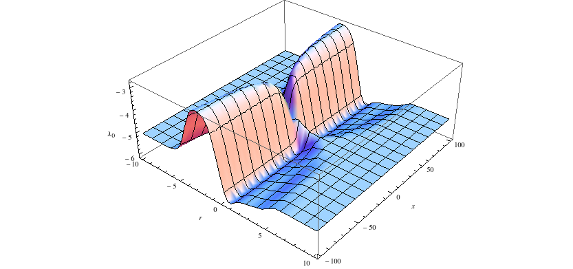
Figure 1: Type II 3D plot of $\lambda_{0}$ (time-like eigenvalue) versus $r$ and $x$ for $\sigma=1,~{}\Lambda=12$.

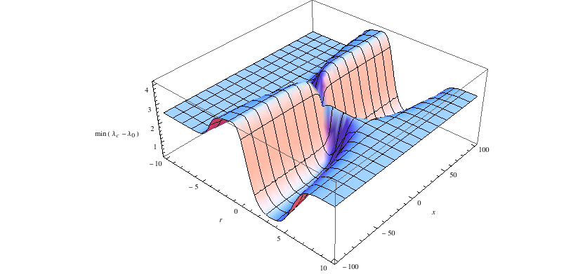
Figure 2: Type II 3D plot of $\min(\lambda_{c}-\lambda_{0})$ versus $r$ and $x$ for $\sigma=1,~{}\Lambda=12$.

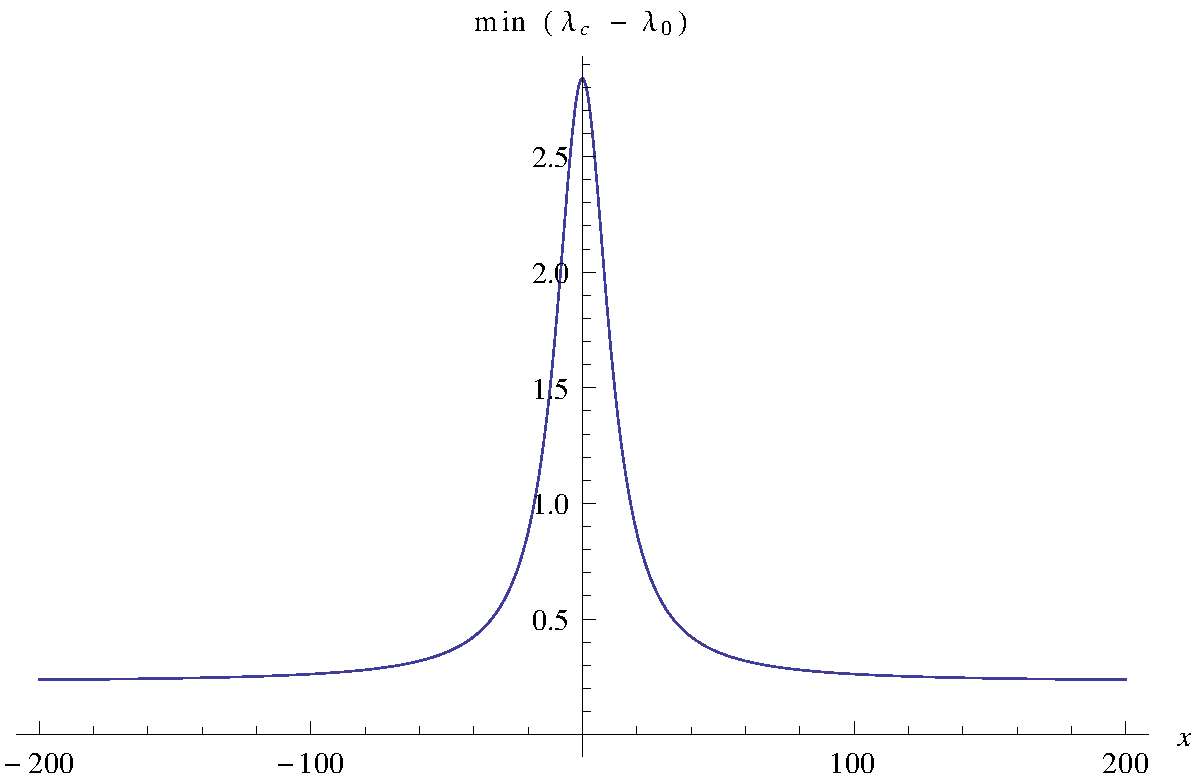
Figure 3: Type II plot of $\min(\lambda_{c}-\lambda_{0})$ versus $x$ at $r=3$ for $\sigma=1,~{}\Lambda=12$.

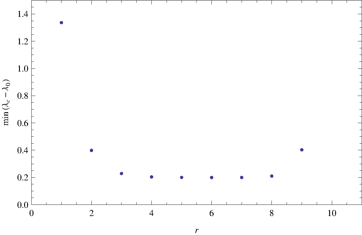
Figure 4: Type II list plot of $\min(\lambda_{c}-\lambda_{0})$ versus $r$ as $x\rightarrow\pm\infty$ for for $\sigma=1,~{}\Lambda=12$.

Let us end this section with one comment. Because of the upper bound on $\sigma$, which arises in order to meet the energy conditions, the metric cannot approach that of Lifshitz space arbitrarily rapidly. The reader might worry that the values of $\sigma$ allowed by this bound are too small to be physically acceptable. To explain this, consider as an example the more familiar case of asymptotically $AdS_{5}$ spacetime. Since a domain wall in $AdS_{5}$ ought to carry positive energy density and pressure, one might expect that the rate at which the metric of such a solution approaches $AdS_{5}$ is governed by the normalizable metric deformations of $AdS_{5}$, and should not be slower. A similar type of argument should also apply to Lifshitz spaces. However, this expectation need not be valid if other fields are also turned on, since these fields can source the metric, and this can lead to a fall-off slower than that expected from the normalizable mode of the metric itself.

4 Types VI, V and III

We now turn to constructing metrics which interpolate from Bianchi Types VI, III and V to Lifshitz. Since our discussion will closely parallel that for Type II above, we will skip some details. We will find that an analysis along the lines above will successfully lead to a class of interpolating metrics for Type VI and Type III, meeting the weak and null energy conditions. However, for reasons which will become clearer below, we do not succeed in finding such an interpolating metric for Type V.

The algebra for a general Type VI spacetime is characterized by one parameter ‘$h$’. Killing vectors and invariant one-forms for Type VI are given in Appendix A of [29] (see also [60]),

$$\xi_{1}=\partial_{y},\quad\xi_{2}=\partial_{z},\quad\xi_{3}=\partial_{x}+y\partial_{y}+hz\partial_{z}$$ (40)

and

$$\omega^{1}=e^{-x}dy,\quad\omega^{2}=e^{-hx}dz,\quad\omega^{3}=dx~{}.$$ (41)

These depend on the parameter $h$.

The Type V algebra is a special case of Type VI, and is obtained by setting $h=1$. The Killing vectors and invariant one-forms can then be obtained from eq.(40) and eq.(41) by setting $h=1$. Similarly the Type III algebra is also a special case obtained by setting $h=0$, with the Killing vectors and one-forms given by setting $h=0$ in the equations above.

To keep the discussion simple, we restrict ourselves to only considering the case $h=-1$ for Type VI, besides also considering the Type V and Type III cases.

The invariant one-forms for Type VI with $h=-1$ are

$$\omega^{1}=e^{-x}dy,\quad\omega^{2}=e^{x}dz,\quad\omega^{3}=dx.$$ (42)

Bianchi Type VI attractor solutions, for the case $h=-1$, were obtained in Section 4.2 of [29] for a system of gravity coupled with a massive gauge field, with an action eq.(14). The solution has a metric,

$$ds_{B}^{2}=R^{2}[dr^{2}-e^{2\beta_{t}r}dt^{2}+e^{2\beta_{1}r}(\omega^{1})^{2}+e^{2\beta_{2}r}(\omega^{2})^{2}+e^{2\beta_{3}r}(\omega^{3})^{2}]$$ (43)

and a gauge field, eq.(17), with the invariant one-forms being given in eq.(42). As in the discussion for Type II we will work in $R=1$ units below. The exponents $\beta_{t},\,\beta_{1},\,\beta_{2},\beta_{3}$ in the solution are then given in terms of $\Lambda$ by

$$\beta_{t} =v,$$ (44)

$$\beta_{1} =\beta_{2}=\frac{(-4+\Lambda-u)v}{24-4\Lambda},$$ (45)

$$\beta_{3} =0,$$ (46)

while the mass and $A_{t}$ are

$$m^{2} =\frac{2}{3}(8-\Lambda+u),$$ (47)

$$A_{t} =\frac{-3v^{2}+u}{6-\Lambda},$$ (48)

where

$$u =\sqrt{-80+8\Lambda+\Lambda^{2}},$$ (49)

$$v =\left[\frac{-28+5\Lambda+u}{6}\right]^{\frac{1}{2}}.$$ (50)

Demanding that $A_{t},m^{2},\beta_{t},\beta_{1},\beta_{2}$ be positive and $u$ be real, we get $\Lambda>6$. The Lifshitz spacetime in the UV is also obtained as a solution of the same system, eq.(14). The metric is given by eq.(22) and the gauge field by eq.(23). The exponent $\beta_{t},{\tilde{\beta}}$ and $A_{t}$ are given in eq.(24), (25) and (26) in terms of $m^{2},\Lambda$. We will take the value of $\Lambda$ to be the same in the IR Type VI and the UV Lifshitz theories. For simplicity we will also take condition eq.(11) to hold so that the exponents along the time direction are the same, accordingly we have denoted both of them as $\beta_{t}$ above.

The strategy we now follow is similar to the Type II case. The interpolating metric is given by eq.(13), which when written out in full becomes

$$\begin{split}ds^{2}&=dr^{2}-e^{2\beta_{t}r}dt^{2}\\ &\quad+\left[\left(\frac{1-\tanh\sigma r}{2}\right)+\left(\frac{1+\tanh\sigma r}{2}\right)e^{2\tilde{\beta}r}\right]dx^{2}\\ &\quad+\left[\left(\frac{1-\tanh\sigma r}{2}\right)e^{2\beta_{1}r-2x}+\left(\frac{1+\tanh\sigma r}{2}\right)e^{2\tilde{\beta}r}\right]dy^{2}\\ &\quad+\left[\left(\frac{1-\tanh\sigma r}{2}\right)e^{2\beta_{2}r+2x}+\left(\frac{1+\tanh\sigma r}{2}\right)e^{2\tilde{\beta}r}\right]dz^{2}.\end{split}$$ (51)

As in the Type II case, we again require that the interpolating metric correctly asymptotes to Type VI in the IR and Lifshitz in the UV. This now imposes the lower bound

$$\sigma>\beta_{1}-\tilde{\beta}=\beta_{2}-\tilde{\beta}.$$ (52)

We remind the reader again that the $r\rightarrow+\infty$ limit is taken while keeping $x$ fixed to obtain this bound.

We take $\Lambda$ (in $R=1$ units) to have the value given in eq.(39). The lower bound for $\sigma$ then becomes, $\sigma>0.0579912$. The matter stress tensor is then calculated as given in eq.(32) and we examine its properties with respect to the energy conditions numerically.

The numerical analysis shows that as $\sigma$ is increased violations of the null energy condition start setting in around $\sigma=1.15993$. The weak energy condition is not violated for smaller values of $\sigma$. Thus, as in the the Type II case, there is a non-vanishing interval for $\sigma$ within which the metric has the correct asymptotic behavior and the weak and null energy conditions are both met.

To illustrate this, consider the case when $\sigma=1$, which lies within this interval. The minimum of the eigenvalues of the spatial eigenvectors turns out to be $\lambda_{2}$, where the eigenvalues are defined in eq.(33)–eq.(37). The plots of $\lambda_{0}$ and $\min(\lambda_{c}-\lambda_{0})=\lambda_{2}-\lambda_{0}$, are given in fig. 5, 6, as a function of the $r,x$ coordinates. We see that the qualitative behavior is similar to that in Type II. $\lambda_{0}$ is always negative. And $\lambda_{2}-\lambda_{0}$ is positive but there is a worrisome region around $r=5$ where this difference of eigenvalues becomes small. We have analyzed this region more carefully further. One finds that for any fixed $r\in[4,9]$ the minimum value for $\lambda_{2}-\lambda_{0}$ is attained as $|x|\rightarrow\infty$ and moreover this minimum value is positive. An analytic expression for this minimum value was also obtained and agrees with the numerical results. This is shown in fig. 7 where this minimum value is plotted as a function of $r$ and shown to be positive. These results establish that the interpolating metric eq.(51) satisfies both the weak and the null energy conditions when $\sigma$ takes values within a suitable range.

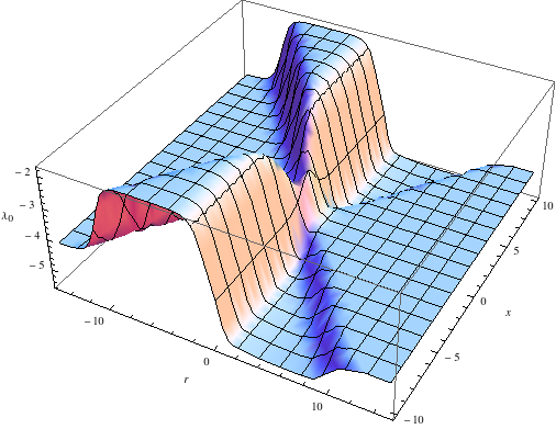
Figure 5: Type VI 3D plot of $\lambda_{0}$ (time-like eigenvalue) versus $r$ and $x$ for $\sigma=1,~{}\Lambda=12$.

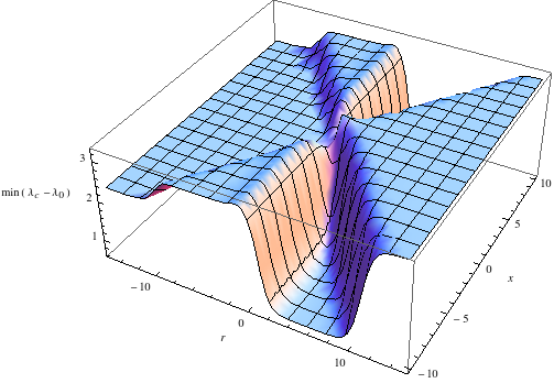
Figure 6: Type VI 3D plot of $\min(\lambda_{c}-\lambda_{0})$ versus $r$ and $x$ for $\sigma=1,~{}\Lambda=12$.

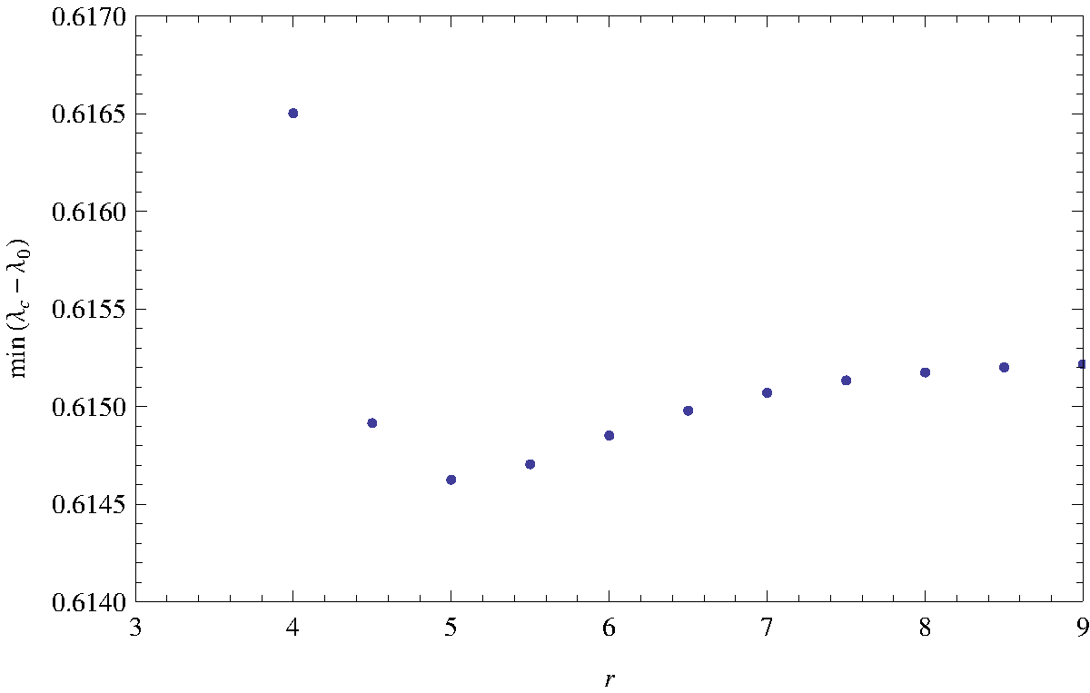
Figure 7: Type VI list plot of $\min(\lambda_{c}-\lambda_{0})$ versus $r$ as $x\rightarrow\pm\infty$ for $\sigma=1,~{}\Lambda=12$.

4.1 Type III

Since the analysis follows that of the Type VI case closely we will be more brief for this case.

The invariant one-forms for Type III, see Appendix A of [29], are given by

$$\omega^{1}=e^{-x}dy,\quad\omega^{2}=dz,\quad\omega^{3}=dx.$$ (53)

Solutions of Type III for the system described by the action eq.(14) exist and have been discussed in section 4.2.2 of [29]. These take the form eq.(43), eq.(17) for the metric and gauge field. The exponents $\beta_{t},\,\beta_{1},\,\beta_{2}$, the gauge field $A_{t}$ and $m^{2}$ (in $R=1$ units) are given by

$$\beta_{t} =v,$$ (54)

$$\beta_{1} =\beta_{3}=0,$$ (55)

$$\beta_{2} =\frac{(-2+\Lambda-u)v}{6-2\Lambda},$$ (56)

$$m^{2} =\frac{1}{2}(4-\Lambda+u),$$ (57)

$$A_{t} =\frac{-4v^{2}+2u}{3-\Lambda},$$ (58)

where

$$u =\sqrt{-8+\Lambda^{2}},$$ (59)

$$v =\frac{\sqrt{-8+3\Lambda+u}}{2}.$$ (60)

Demanding that $A_{t},m^{2},\beta_{t},\beta_{2}$ be positive and $u$ to be real, we get $\Lambda>3$. To obtain the desired interpolation from a Bianchi Type III solution to Lifshitz, we follow the strategy adopted in case of Type II, VI, above, and consider the following interpolating metric:

$$\begin{split}ds^{2}&=dr^{2}-e^{2\beta_{t}r}dt^{2}\\ &\quad+\left[\left(\frac{1-\tanh\sigma r}{2}\right)+\left(\frac{1+\tanh\sigma r}{2}\right)e^{2\tilde{\beta}r}\right]dx^{2}\\ &\quad+\left[\left(\frac{1-\tanh\sigma r}{2}\right)e^{-2x}+\left(\frac{1+\tanh\sigma r}{2}\right)e^{2\tilde{\beta}r}\right]dy^{2}\\ &\quad+\left[\left(\frac{1-\tanh\sigma r}{2}\right)e^{2\beta_{2}r}+\left(\frac{1+\tanh\sigma r}{2}\right)e^{2\tilde{\beta}r}\right]dz^{2}.\end{split}$$ (61)

Requiring this interpolating metric to correctly asymptote to Type VI in the IR and Lifshitz in the UV imposes the following lower bound: $\sigma>\beta_{2}-\tilde{\beta}$. We choose $\Lambda=12$ in $R=1$ units. The lower bound for $\sigma$ then becomes, $\sigma>0.0456046$.

Furthermore, we numerically find that violations of the null energy condition start setting in around $\sigma=0.40108$. The weak energy condition is not violated for smaller values of $\sigma$. Thus, we find once again that there is a range of values for $\sigma$ for which the metric asymptotes to the required forms and for which the weak and null energy conditions are preserved.

To illustrate this, we choose $\sigma=0.3$ which lies in the allowed region. The plots of $\lambda_{0}$ and $\min(\lambda_{c}-\lambda_{0})=\lambda_{2}-\lambda_{0}$, where $\lambda_{0}$ and $\lambda_{2}$ are as defined in eq.(33) and eq.(35), are given in fig. 8 and fig. 9. We see that $\lambda_{0}$ is always negative. And $\lambda_{2}-\lambda_{0}$ is positive but this difference becomes small near $r\sim 10-15$ as $x\rightarrow-\infty$. We examined this region in more detail and find that for any fixed $r$ in this region $\lambda_{2}-\lambda_{0}$ attains its minimum value as $x$ is varied for $x\rightarrow-\infty$ and this minimum value is indeed positive. An analytic expression for this minimum value was obtained, and agrees with the numerical analysis. In fig 10 we plot this minimum value, attained when $x\rightarrow-\infty$, for $\lambda_{2}-\lambda_{0}$ against $r$. We see that the minimum value is positive. These results establish that the interpolating metric eq.(61) in the Type III case also meets the weak and null energy conditions for a suitable range of $\sigma$ values.

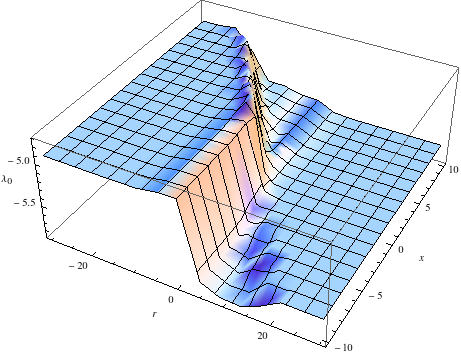
Figure 8: Type III 3D plot of $\lambda_{0}$ (time-like eigenvalue) versus $r$ and $x$ for $\sigma=0.3,~{}\Lambda=12$.

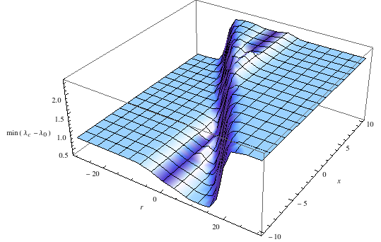
Figure 9: Type III 3D plot of $\min(\lambda_{c}-\lambda_{0})$ versus $r$ and $x$ for $\sigma=0.3,~{}\Lambda=12$.

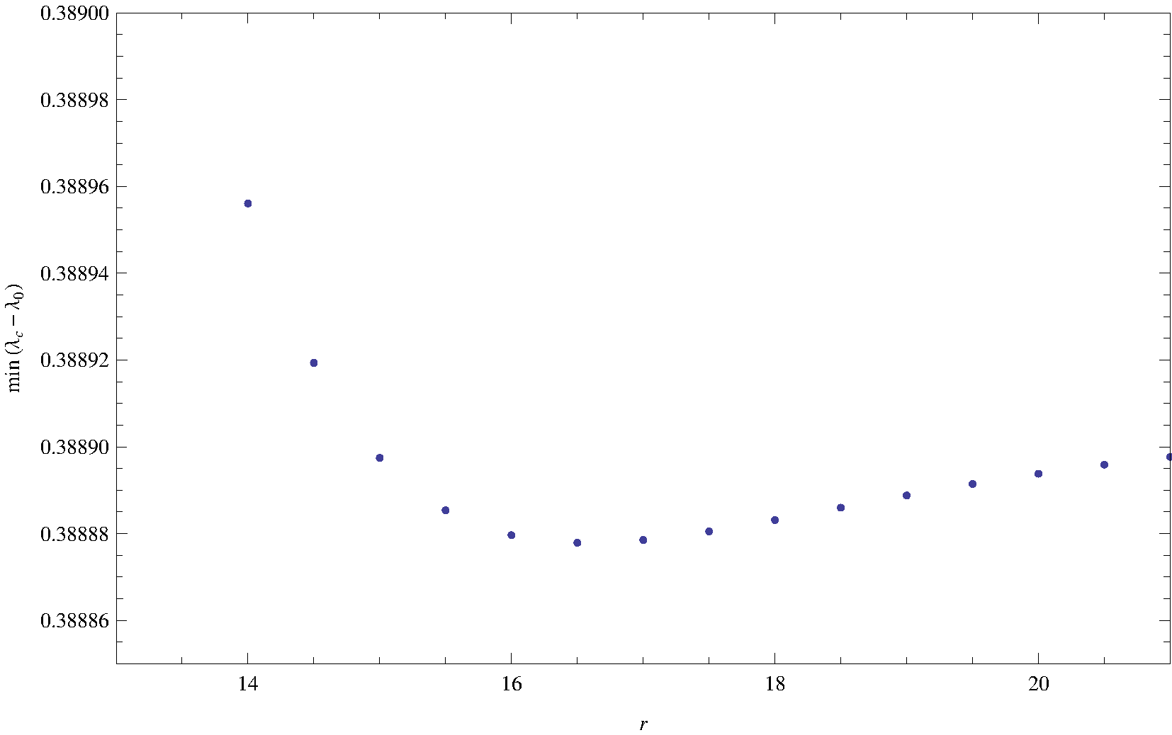
Figure 10: Type III list plot of $\min(\lambda_{c}-\lambda_{0})$ versus $r$ as $x\rightarrow-\infty$ for $\sigma=0.3,~{}\Lambda=12$.

4.2 Type V

The invariant one-forms in the Type V case are

$$\omega^{1}=e^{-x}dy,\quad\omega^{2}=e^{-x}dz,\quad\omega^{3}=dx.$$ (62)

Solutions of Type V for the system, eq.(14) take the form eq.(8), eq.(17). The parameters, $\beta_{t},\,\beta_{1},\,\beta_{2},\,m^{2},\,A_{t},$ are given by

$$\beta_{t} =\sqrt{-4+\Lambda},$$ (63)

$$\beta_{1}=\beta_{2}=\beta_{3} =0,$$ (64)

$$m^{2} =0,$$ (65)

$$A_{t} =\frac{2(6-\Lambda)}{4-\Lambda}.$$ (66)

Demanding that $A_{t},\beta_{t}$ be positive and real respectively, we get $\Lambda>6$. Starting from this metric in the IR one would like to consider a metric of the form eq.(13) which interpolates to Lifshitz space in the UV. However, it turns out that in this case interpolations of the the type eq.(61) violate the null energy condition for all values of $\sigma$.

The failure of the interpolating metric to work in this case can in fact be understood analytically. It is tied to the fact that the Type V solution has one important difference with the other kinds of solutions, Type II, VI, III, studied above. Here, it turns out that the smallest eigenvalue of $T^{(\mathrm{matter})\mu}_{\nu}$ corresponding to a space-like eigenvector, $\min(\lambda_{c}),c=1,2,3,4$, is exactly equal to the eigenvalue corresponding to the time-like eigenvector, $\lambda_{0}$, and thus the null energy condition eq.(2) is met as an equality. This case is therefore much more delicate.

In fact, a perturbative analysis reveals that once the Type V metric is deformed by considering the full interpolating metric given in eq.(61), the splitting which results as $r\rightarrow-\infty$ goes in the wrong direction, making $\min(\lambda_{c})-\lambda_{0}<0$ for any value of $\sigma$, leading to a violation of the null energy condition.

5 From Type IX To $AdS_{2}\times S^{3}$

The symmetry algebra for Bianchi Type IX is $SO(3)$ and its natural action is on a compact space corresponding to a squashed $S^{3}$. Therefore, for Type IX it is natural to explore interpolations going from a Type IX attractor geometry to $AdS_{2}\times S^{3}$ instead of $AdS_{2}\times R^{3}$ or Lifshitz.

The strategy we use for finding such an interpolation is different from what was used in the cases above. It is motivated by the fact that the $SO(3)$ symmetry for Type IX is a subgroup of the symmetries of $S^{3}$, $SO(3)\times SO(3)$. The interpolating metric we consider will therefore be obtained by introducing a deformation parameter which allows the spatial components of the metric to go from that of a squashed $S^{3}$ in the IR to the round $S^{3}$ in the UV. This is somewhat akin to what was done in [29] to find an interpolation between Type VII and Type I.

The invariant one-forms for Bianchi Type IX are

$$\omega^{1} =-\sin(z)\,dx+\sin(x)\cos(z)\,dy,$$

$$\omega^{2} =\cos(z)\,dx+\sin(x)\sin(z)\,dy,$$

$$\omega^{3} =\cos(x)\,dy+dz.$$

One finds that a Type IX attractor solution arises in a system of Einstein gravity with the cosmological constant $\Lambda$, coupled to two gauge fields, $A_{1},A_{2}$ with action

$$S=\int d^{5}x\sqrt{-g}\left(R+\Lambda-\frac{1}{4}F_{1}^{2}-\frac{1}{4}F_{2}^{2}-\frac{1}{4}m^{2}A_{2}^{2}\right).$$ (67)

Note that $A_{1}$ is massless while $A_{2}$ has $(\mathrm{mass})^{2}=m^{2}$.

In this solution the metric is given by

$$ds^{2}=R^{2}[dr^{2}-e^{2\beta_{t}r}dt^{2}+(\omega^{1})^{2}+(\omega^{2})^{2}+\ \lambda\ (\omega^{3})^{2}]$$ (68)

and the two gauge fields are

$$A_{1}=\sqrt{A_{t}}\,e^{\beta_{t}r}dt,\hskip 14.22636ptA_{2}=\sqrt{A_{s}}\,\omega^{3}=\sqrt{A_{s}}\,(\cos(x)dy+dz).$$ (69)

Note that $\lambda$ in eq.(68) is the deformation parameter we had mentioned above.

In $R=1$ units, the equations of motion which follow from eq.(67) give rise to the following relations,

$$m^{2}=-2\lambda, A_{t}=\frac{2(-\lambda+2\Lambda+4)}{-\lambda+2\Lambda+3},$$ (70)

$$A_{s}=1-\lambda, \beta_{t}=\left[\frac{-\lambda+2\Lambda+3}{2}\right]^{\frac{1}{2}}.$$ (71)

These relations can be thought of as determining $A_{s},A_{t},\beta_{t},\lambda$ in terms of $\Lambda$ and $m^{2}$.

Note that the conditions $A_{s},A_{t}\geq 0,\,\Lambda>0$ imply, from eq.(70) and eq.(71), the relation

$$\lambda\leq 1.$$ (72)

It is easy to see that for $\lambda=1$, this solution becomes $AdS_{2}\times S^{3}$, and for any other value of $\lambda$ between 0 and 1, it is Type IX.

Let us make one comment before proceeding. Eq.(70) and Eq.(71) give four relations and at first it might seem that they determine the four parameters $A_{t},A_{s},\lambda,\beta_{t}$ and therefore determine the solution completely. However, since we have set the radius $R=1$, this is not the case and the solution in fact contains one undetermined parameter. This becomes clear if we consider the $\lambda=1$ case, where $A_{s}=0$ and the massive gauge field vanishes. The resulting solution is $AdS_{2}\times S^{3}$ which is the near-horizon extremal RN solution. This solution has one free parameter, which we can take to be $A_{t}$, the value of the massless gauge field which determines the electric field of this gauge field. Or we can take it to be $R$. In the interpolation below, we will take the free parameter to be $R$, and set $R=1$, keeping its value fixed as the radial coordinate $r$ varies.

It turns out that for the solution given above in eq.(68), eq.(69), eq.(70), eq.(71), for any given $\lambda$, the null energy condition is satisfied but as an equality, with the smallest eigenvalue of a space-like eigenvector of $T^{(\mathrm{matter})\mu}_{\nu}$, $\min(\lambda_{c})$, being equal to the eigenvalue for the time-like eigenvector, $\lambda_{0}$. This is analogous to what we saw above in the Type V case. However, here because the symmetries involved are different, we can choose another kind of interpolation, as mentioned in the beginning of this section.

We do this by taking $\lambda$ to be a function of $r$ of the form

$$\lambda(r)=C+(1-C)\left({1+\tanh(\sigma r)\over 2}\right)$$ (73)

where $C$, and $\sigma$ are constants, with $0<C<1$, to meet eq.(72). We find that the degeneracy between $\min(\lambda_{c}),\lambda_{0}$ is now lifted. Unlike the Type V case though, this lifting occurs so that $\min(\lambda_{c})-\lambda_{0}>0$, if $\sigma$ is sufficiently small, thus preserving the null energy condition, eq.(2). If $\sigma$ becomes bigger than a critical value, violations of the NEC set in.

For example, for the choice of $\Lambda=12$, and $C=0.5$ we find that the energy conditions are met for a range of $\sigma$ up to $\sigma_{\mathrm{crit}}=1.82$. For $0<\sigma\leq 1.82$ and $C=0.5$ both eq.(4), eq.(5) are met, so that the interpolating metric above satisfies the WEC and hence also the NEC.

For $C=0.5,~{}\sigma=0.5$, the results are summarized in fig. 11 and 12. Fig. 11 shows that $\lambda_{0}$ satisfies the condition $\lambda_{0}<0$. And fig. 12 shows that $\min(\lambda_{c}-\lambda_{0})>0$. As $r\rightarrow\pm\infty$ the interpolation approaches a solution of the type considered in eq.(68), eq.(69), and the value of $\min(\lambda_{c}-\lambda_{0})\rightarrow 0$. However, we have verified that at both ends, $r\rightarrow\pm\infty$, $\min(\lambda_{c}-\lambda_{0})$ approaches zero from above so that the NEC continues to hold. Together, these results imply that $T^{(\mathrm{matter})\mu}_{\nu}$ satisfies the weak energy condition, and therefore also the null energy condition.

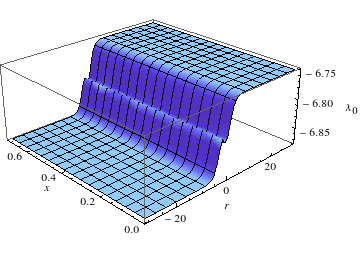
Figure 11: Type IX 3D plot of $\lambda_{0}$ (time-like eigenvalue) versus $r$ and $x$ for $C=0.5,~{}\sigma=0.5,~{}\Lambda=12$.

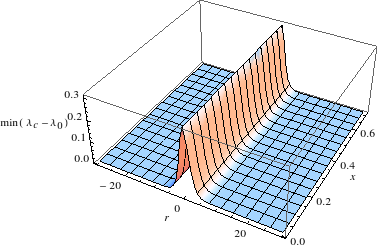
Figure 12: Type IX 3D plot of $\min(\lambda_{c}-\lambda_{0})$ versus $r$ and $x$ for $C=0.5,~{}\sigma=0.5,~{}\Lambda=12$.

6 C-function

In this section, we investigate a large class of geometries of the form

$$ds^{2}=-g_{tt}(r)dt^{2}+dr^{2}+g_{ij}(x^{i},r)dx^{i}dx^{j}$$ (74)

which interpolate between two Bianchi attractor spacetimes. The Bianchi attractors arise at the UV and IR ends, $r\rightarrow\pm\infty$ respectively, where the geometry takes the scale invariant form, eq.(8), with the exponents $\beta_{t},\beta_{i}$ being constant and positive. The UV and IR ends are defined by the redshift factor, $g_{tt}$, which decreases from the UV to the IR.

We find that as long as the matter sourcing the geometry satisfies the null energy condition, the area element of the submanifold spanned by the $x^{i}$ coordinates (at constant $t,r$) monotonically decreases with $r$, obtaining its minimum value in the IR. For a Bianchi attractor, eq.(8), the area element is proportional to $e^{\sum_{i}\beta_{i}r}$ and diverges in the UV, $r\rightarrow\infty$, while vanishing in the IR, $r\rightarrow-\infty$. The only exception is when the exponents $\beta_{i}$ all vanish, as happens for example in $AdS_{2}\times R^{3}$ space, in which case the area element becomes a non-zero constant. We also find an additional function, which we will refer to as the C-function below, which is monotonically decreasing from the UV to the IR. For an AdS attractor, this function attains a constant value and is the central charge. For other Bianchi attractors meeting a specific condition, given in eq.(91) below, this function also flows to a constant in the near-horizon region. More generally, when this specific condition is not met, the function either vanishes or diverges as $r\rightarrow\pm\infty$. All of these results are most easily derived by applying Raychaudhuri’s equation to an appropriately chosen set of null geodesics in the geometry, eq.(74).

Note that the flows we study include interpolations between two AdS spacetimes which at intermediate values of $r$ can break not only Lorentz invariance but also spatial rotational invariance and translational invariance. As long as the UV and IR geometries are AdS, our results imply that the IR central charge must be smaller than the UV one. Our results therefore lead to a generalization of the holographic C-theorem for flows between conformally invariant theories which can also break boost, rotational and translational symmetries. This is in contrast to much of the discussion in the literature so far, which has considered only Lorentz invariant flows.

Besides the area element and the C-function mentioned above, and of course monotonic functions of these, for example, powers of the area element or the C-function, we do not find any other function which in general would necessarily be monotonic as a consequence of the null energy condition. As was mentioned above, both the area element and the C-function do not in general attain finite non-vanishing values in the asymptotic Bianchi attractor regions. This suggests that for Bianchi attractors in general, no analogue of a finite, non-vanishing, central charge can be defined which is monotonic under RG flow. This conclusion should apply for example to general Lifshitz spacetimes (see also a discussion of these cases in [61]). When the Bianchi attractor meets the specific condition of eq.(91), the C-function does become a finite constant and the analogue of the central charge can be defined. Understanding this constant in the field theory dual to the Bianchi attractor would be a worthwhile thing to do.

6.1 The Analysis

We now turn to describing the analysis in more detail. Our notation will follow that of [62], Section 9.2. The analysis is also connected to the discussion of a C-function in [63]. A nice discussion of the C-function in AdS space can be found in Section 4.3.2 of [64]. For discussions of renormalization group flows in the context of the AdS/CFT correspondence, see [65, 66, 67, 68, 69]. The earliest proofs of holographic C-theorems appear in [70], [71], and our strategy is a generalization of the one employed there.

We start with a spacetime described by the metric, eq.(74), and consider a $3$-dimensional submanifold spanned by the $x^{i}$ coordinates for any fixed $r,t$. Next, we consider a family of null geodesics which emanate from all points of this submanifold. If $n^{a}$ is the tangent vector of the null geodesic, with $a$ taking the values $a=t,r,i=1,2,3$, then the geodesics we consider have $n^{i}=0$ so that they correspond to motion only in the radial direction. Both the radially in-going and out-going families of this type form a congruence. To arrive at our results, it is enough to consider any one of them and we consider the radial out-going geodesics below. The time-like component of the vectors in this congruence, $n_{t}$, is a constant which we can set to unity,

$$n_{t}=1.$$ (75)

Then for the radially outgoing geodesics

$$n^{r}={dr\over d\lambda}={1\over\sqrt{g_{tt}}},$$ (76)

where $\lambda$ is the affine parameter along the geodesic.

Now we take the tensor field

$$B_{ab}=\nabla_{b}n_{a}$$ (77)

and consider its components for $a,b=i,j=1,2,3$. In the notation of [62], this gives us the components of $\hat{B}_{ab}$. It is easy to see that

$$B_{ij}=-\Gamma^{c}_{ij}n_{c}={1\over 2}{\partial_{r}g_{ij}\over g_{tt}}$$ (78)

and thus $B_{ij}$ is symmetric so that the twist of the congruence vanishes. The expansion of the congruence, denoted by $\theta$, is then

$$\theta={1\over 2}\partial_{r}g_{ij}{g^{ij}\over\sqrt{g_{tt}}}=\partial_{r}(\ln A){1\over\sqrt{g_{tt}}},$$ (79)

where we have introduced the notation

$$A\equiv\sqrt{\det(g_{ij})}$$ (80)

to denote the area element of the hypersurface spanned by the $x^{i}$ coordinates for any constant $r,t$.

From eq.(79) and eq.(76) we get that

$${d\theta\over d\lambda}={1\over\sqrt{g_{tt}}}\partial_{r}\left({\partial_{r}\ln A\over\sqrt{g_{tt}}}\right).$$ (81)

Raychaudhuri’s equation then gives

$${d\theta\over d\lambda}=-{1\over 3}\theta^{2}-\hat{\sigma}_{ab}\hat{\sigma}^{ab}-R_{cd}n^{c}n^{d}$$ (82)

since the twist $\hat{\omega}_{ab}=0$. Note that the coefficient of the first term on the RHS is ${1\over 3}$ and not ${1\over 2}$ since we are in $4+1$ dimensions and not $3+1$ dimensions.

If the matter sourcing the geometry satisfies the null energy condition, the Ricci curvature satisfies the relation $R_{cd}n^{c}n^{d}\geq 0$, leading to the conclusion from eq.(82) that ${d\theta\over d\lambda}<0$. From eq.(81), this in turn leads to

$$\partial_{r}\left({\partial_{r}\ln A\over\sqrt{g_{tt}}}\right)<0.$$ (83)

In the UV, $r\rightarrow\infty$,

$${\partial_{r}\ln A\over\sqrt{g_{tt}}}=\sum_{i}\beta_{i}e^{-\beta_{t}r}>0$$ (84)

where $\beta_{i},\beta_{t}$ are the exponents corresponding to the UV attractor. It then follows from eq.(83) that for all values of $r$, ${\partial_{r}\ln A\over\sqrt{g_{tt}}}>0$, and thus

$$\partial_{r}\ln A>0.$$ (85)

This leads to our first result: the area element $A$, defined in eq.(80), decreases monotonically from the UV, $r\rightarrow\infty$, to the IR, $r\rightarrow-\infty$.

Raychaudhuri’s equation, eq.(82) also leads to the conclusion that

$${d\theta\over d\lambda}+{1\over 3}\theta^{2}\leq 0,$$ (86)

if the matter satisfies the null energy condition. From eq.(79), eq.(81) this leads to

$$\partial_{r}\left({(\partial_{r}\ln A)A^{1/3}\over\sqrt{g_{tt}}}\right)<0.$$ (87)

A monotonically decreasing function from the UV to the IR is therefore given by

$$C=\left({\sqrt{g_{tt}}\over(\partial_{r}\ln A)A^{1/3}}\right)^{3}.$$ (88)

For a Bianchi attractor with exponents $\beta_{t},\beta_{i}$, $C$ becomes

$$C\propto\left({e^{(\beta_{t}-\bar{\beta})r}\over 3\bar{\beta}}\right)^{3},$$ (89)

where we have defined

$$\bar{\beta}={1\over 3}\sum_{i}\beta_{i}.$$ (90)

The overall power of $3$ in the definition of $C$, eq.(88), is chosen so that in AdS space, where $\beta_{i}=\beta_{t}$ and $C$ is a constant, it agrees with the usual definition of the central charge up to an overall coefficient. More generally, $C$ also becomes a constant for any Bianchi attractor meeting the condition

$$\beta_{t}=\bar{\beta}={1\over 3}\sum_{i}\beta_{i}$$ (91)

and now takes a value

$$C\propto{1\over\left(\sum_{i}\beta_{i}\right)^{3}}.$$ (92)

However, for the general case of a Bianchi attractor which does not meet the condition in eq.(91), $C$ does not attain a constant value. In such situations, for $C$ to be monotonically decreasing towards the IR or constant, we need $(\beta_{t}-\bar{\beta})\geq 0$. Thus, we find that if the attractor arises in the IR, then our $C$ vanishes. On the other hand, if the attractor arises in the UV, it diverges.

7 Conclusions

In this paper, we constructed a class of smooth metrics which interpolate from various Bianchi attractor geometries in the IR to Lifshitz spaces or $AdS_{2}\times S^{3}$ in the UV. We did not show that these interpolating metrics arise as solutions to Einstein gravity coupled with suitable matter field theories. However, for Bianchi Types II, VI (with parameter $h=-1$), III and IX, we did show that were these geometries to arise as solutions to Einstein’s equations, the required matter would not violate the weak or null energy conditions. It is well known that the Lifshitz spaces (which are in fact attractors of Bianchi Type I) or $AdS_{2}\times S^{3}$ geometry in turn can be connected to $AdS_{5}$ in the ultraviolet, with no non-normalizable deformation for the metric being turned on in the asymptotic $AdS_{5}$ region. Thus, our results establish that there is no barrier, at least at the level of energy conditions, to having a smooth interpolating metric arise as a solution of the Einstein equations sourced by reasonable matter, which connects the various Bianchi classes mentioned above with asymptotic $AdS_{5}$ space. We should mention here that for Type VII geometries, which were not investigated in this paper, solutions with reasonable matter which interpolate from the attractor region to $AdS_{2}\times R^{3}$ or $AdS_{5}$ are already known to exist [29].

The absence of any non-normalizable metric deformations in the asymptotic $AdS_{5}$ region in our interpolations suggests that the Bianchi attractor geometries can arise as the dual description in the IR of field theories which live in flat space. The anisotropic and homogeneous phases in these field theories, described by the Bianchi attractor regions, could arise either due to a spontaneous breaking of rotational invariance or due to its breaking by sources other than the metric in the field theory. We expect both possibilities to be borne out. For spin density waves, which correspond to Type VII, indeed this is already known to be true [28, 29].

Finding such interpolating metrics as solutions to Einstein’s equations is not easy, as was mentioned in the introduction, since it requires solving coupled partial differential equations in at least two variables. We hope that the results presented here will provide some further motivation to try and address this challenging problem. Perhaps it might be best to first look for supersymmetric domain walls interpolating between different Bianchi types, since for such solutions, working with first-order equations often suffices.

We also note that our smooth interpolating metric which interpolates from Bianchi Type V to Lifshitz failed to satisfy the null energy conditions. Our failure in this case may be due to the restricted class of functions we used to construct the interpolating metrics or it might suggest a more fundamental constraint. We leave a more detailed exploration of this issue for the future.

Towards the end of the paper, we explored whether a C-function exists for flows between two Bianchi attractor geometries. As long as the matter sourcing the geometry meets the null energy condition, we found that a function can be defined which is monotonically decreasing from the UV to the IR. In AdS space, this function becomes the usual central charge. More generally though, unless the Bianchi attractor meets a specific condition relating the exponents $\beta_{i},\beta_{t}$ which characterize it, the function we have identified does not attain a finite, non-vanishing constant value in the attractor geometry. The absence of a general monotonic function which is non-vanishing and finite in the attractor spacetime suggests that no analogue of a central charge, which is monotonic under RG flow, can be defined in general for field theories dual to the Bianchi attractors. For flows between AdS spacetimes, on the other hand, our analysis implies that the central charge decreases even under RG flows which break boost, rotational and translational invariance.

Acknowledgements

We thank Sarah Harrison, Nori Iizuka, Prithvi Narayan, Ashoke Sen, Nilanjan Sircar and Huajia Wang for discussions. S.P.T. acknowledges support from the J. C.  Bose Fellowship, Department of Science and Technology, Government of India. S.K. and S.P.T. acknowledge the hospitality of the Simons Symposium on Quantum Entanglement, where some of this research was carried out. N.K., R.S. and S.P.T. acknowledge support from the Government of India and most of all are grateful to the people of India for generously supporting research in string theory. A.S. would like to thank the Department of Physics, Indian Institute of Technology – Bombay, for its support. S.K. is supported by the National Science Foundation under grant no. PHY-0756174, the Department of Energy under contract DE-AC02-76SF00515, and the John Templeton Foundation.

Appendix A The Weak and Null Energy Conditions

We shall now review the weak and null energy conditions in detail. The weak energy condition (WEC) stipulates that the local energy density as observed by a time-like observer is nonnegative. In other words, if $u^{\mu}$ are the components of a time-like vector, we must have $T_{\mu\nu}u^{\mu}u^{\nu}\geq 0$ everywhere, with $T_{\mu\nu}$ being the components of the stress tensor. Note that if we raise one of the indices of $T_{\mu\nu}$ to get $T^{\mu}_{\nu}$, we could interpret the stress tensor as a linear transformation $T$ that acts on the components of a vector $u$ via $(Tu)^{\mu}=T^{\mu}_{\nu}u^{\nu}$.

The WEC now simply becomes $\langle u,Tu\rangle\geq 0$, where the angle brackets denote the inner product with respect to the metric. Since $T$ is a linear transformation from a vector space to itself, it makes sense to talk of the eigenvalues and eigenvectors of $T$. In particular, if $u$ is a time-like eigenvector which is normalized so that $\langle u,u\rangle=-1$ and which belongs to some eigenvalue $\lambda$ (not to be confused with the $\lambda$ parameter we had introduced in the interpolating metric), then we have

$$\langle u,Tu\rangle=\lambda\langle u,u\rangle=-\lambda.$$ (93)

Thus, a necessary condition for the WEC to hold is that the eigenvalues corresponding to all time-like eigenvectors of $T$ be non-positive.

Note that this isn’t a sufficient condition for the WEC to hold. To go further, let us first note that $T$ is self-adjoint:

$$\langle u,Tv\rangle=T_{\mu\nu}u^{\mu}v^{\nu}=\langle Tu,v\rangle.$$

However, it does not follow from this property that $T$ is diagonalizable and that its eigenvalues are necessarily real, since the inner product is indefinite in a Lorentzian metric. For the metrics we deal with in the paper, we fortunately do not have to deal with this complication because, it turns out that in all the cases we analyze, $T$ does turn out to be diagonalizable with real eigenvalues. Accordingly, we restrict our discussion to this case below.

It then follows that there exists a vierbein $\{u_{0},u_{1},u_{2},u_{3},u_{4}\}$ consisting of the eigenvectors of $T$, which is orthonormal in the sense that $\langle u_{a},u_{b}\rangle=\eta_{ab}$. If we let $Tu_{a}=\lambda_{a}u_{a}$, then our claim is that the WEC is equivalent to the following statement: $\lambda_{0}\leq 0$ and $\lvert\lambda_{0}\rvert+\lambda_{c}\geq 0$ for $c=1,2,3,4$.

To prove necessity, we note that we have already shown that $\lambda_{0}\leq 0$. Now, for an arbitrary time-like vector of the form $v=Au_{0}+Bu_{c}$, where $c$ can be 1, 2, 3 or 4, we have $\langle v,v\rangle=-A^{2}+B^{2}<0$. By the WEC we have

$$\langle v,Tv\rangle=|\lambda_{0}|A^{2}+\lambda_{c}B^{2}\geq 0.$$

If we let $\epsilon=A^{2}-B^{2}$, the above can rewritten as

$$(|\lambda_{0}|+\lambda_{c})B^{2}+\epsilon|\lambda_{0}|\geq 0.$$

Since $v$ is arbitrary, $\epsilon$ can be an arbitrarily small positive real number. It follows that $\lvert\lambda_{0}\rvert+\lambda_{c}\geq 0$ for $c=1,2,3,4$.

To prove sufficiency, we note that a generic time-like vector $v$ may be given by

$$v=Au_{0}+Bu_{1}+Cu_{2}+Du_{3}+Eu_{4}.$$

where the coefficients are subject to the following

$$A^{2}>B^{2}+C^{2}+D^{2}+E^{2}.$$

The conditions $\lambda_{0}\leq 0$ and $\lvert\lambda_{0}\rvert+\lambda_{c}\geq 0$ for $c=1,2,3,4$ hence guarantee that

$$\langle v,Tv\rangle =|\lambda_{0}|A^{2}+\lambda_{1}B^{2}+\lambda_{2}C^{2}+\lambda_{3}D^{2}+\lambda_{4}E^{2}$$

$$\geq|\lambda_{0}|(B^{2}+C^{2}+D^{2}+E^{2})+\lambda_{1}B^{2}+\lambda_{2}C^{2}+\lambda_{3}D^{2}+\lambda_{4}E^{2}$$

$$=(\lvert\lambda_{0}\rvert+\lambda_{1})B^{2}+(\lvert\lambda_{0}\rvert+\lambda_{2})C^{2}+(\lvert\lambda_{0}\rvert+\lambda_{3})D^{2}+(\lvert\lambda_{0}\rvert+\lambda_{4})E^{2}$$

$$\geq 0.$$

In fact, we can go further and easily show this implies the null energy condition (which states that $\langle n,Tn\rangle\geq 0$ for all null vectors $n$ everywhere) by following the same outline as the proof above. We note that a generic null vector $n$ may be given by

$$n=Au_{0}+Bu_{1}+Cu_{2}+Du_{3}+Eu_{4},$$

where the coefficients are subject to the following

$$A^{2}=B^{2}+C^{2}+D^{2}+E^{2}.$$

The conditions $\lambda_{0}\leq 0$ and $\lvert\lambda_{0}\rvert+\lambda_{c}\geq 0$ for $c=1,2,3,4$ hence guarantee that

$$\langle n,Tn\rangle =|\lambda_{0}|A^{2}+\lambda_{1}B^{2}+\lambda_{2}C^{2}+\lambda_{3}D^{2}++\lambda_{4}E^{2}$$

$$=\lambda_{0}|(B^{2}+C^{2}+D^{2}+E^{2})+\lambda_{1}B^{2}+\lambda_{2}C^{2}+\lambda_{3}D^{2}+\lambda_{4}E^{2}$$

$$=(\lvert\lambda_{0}\rvert+\lambda_{1})B^{2}+(\lvert\lambda_{0}\rvert+\lambda_{2})C^{2}+(\lvert\lambda_{0}\rvert+\lambda_{3})D^{2}+(\lvert\lambda_{0}\rvert+\lambda_{4})E^{2}$$

$$\geq 0,$$

which is the null energy condition (NEC). Thus, in terms of the eigenvalues, the NEC is equivalent to the following statement: $-\lambda_{0}+\lambda_{c}\geq 0$ for $c=1,2,3,4$ where $\lambda_{0}$ is the eigenvalue corresponding to the time-like eigenvector and $\lambda_{c}$ corresponds to any of the space-like eigenvectors.

To summarize the above observations:

1. For the WEC, it suffices to have (i) $\lambda_{0}\leq 0$ and (ii) $\lvert\lambda_{0}\rvert+\lambda_{c}\geq 0$ for $c=1,2,3,4$.

2. For the NEC, it suffices to have $-\lambda_{0}+\lambda_{c}\geq 0$ for $c=1,2,3,4$, where $\lambda_{0}$ is the eigenvalue corresponding to the time-like eigenvector and $\lambda_{c}$ corresponds to any of the space-like eigenvectors.

References

- [1] S. A. Hartnoll, “Lectures on holographic methods for condensed matter physics,” arXiv:0903.3246 [hep-th].
- [2] C. P. Herzog, “Lectures on Holographic Superfluidity and Superconductivity,” J. Phys. A 42, 343001 (2009) [arXiv:0904.1975 [hep-th]].
- [3] J. McGreevy, “Holographic duality with a view toward many-body physics,” Adv. High Energy Phys. 2010, 723105 (2010) [arXiv:0909.0518 [hep-th]].
- [4] S. Sachdev, “What can gauge-gravity duality teach us about condensed matter physics?,” Ann. Rev. Condensed Matter Phys. 3, 9 (2012) [arXiv:1108.1197 [cond-mat.str-el]].
- [5] S. S. Gubser, “Breaking an Abelian gauge symmetry near a black hole horizon,” Phys. Rev. D 78, 065034 (2008) [arXiv:0801.2977 [hep-th]].
- [6] S. A. Hartnoll, C. P. Herzog and G. T. Horowitz, “Building a Holographic Superconductor,” Phys. Rev. Lett. 101, 031601 (2008) [arXiv:0803.3295 [hep-th]].
- [7] S. A. Hartnoll, C. P. Herzog and G. T. Horowitz, “Holographic Superconductors,” JHEP 0812, 015 (2008) [arXiv:0810.1563 [hep-th]].
- [8] G. T. Horowitz, “Theory of Superconductivity,” Lect. Notes Phys. 828, 313 (2011) [arXiv:1002.1722 [hep-th]].
- [9] S. Kachru, X. Liu and M. Mulligan, “Gravity Duals of Lifshitz-like Fixed Points,” Phys. Rev. D 78, 106005 (2008) [arXiv:0808.1725 [hep-th]].
- [10] M. Taylor, “Non-relativistic holography,” arXiv:0812.0530 [hep-th].
-
[11]
K. Goldstein, S. Kachru, S. Prakash and S. P. Trivedi,
“Holography of Charged Dilaton Black Holes,”
JHEP 1008, 078 (2010)
[arXiv:0911.3586 [hep-th]];
K. Goldstein, N. Iizuka, S. Kachru, S. Prakash, S. P. Trivedi and A. Westphal, “Holography of Dyonic Dilaton Black Branes,” JHEP 1010, 027 (2010) [arXiv:1007.2490 [hep-th]]. -
[12]
C. Charmousis, B. Gouteraux, B. S. Kim, E. Kiritsis and R. Meyer,
“Effective Holographic Theories for low-temperature condensed matter systems,”
JHEP 1011, 151 (2010)
[arXiv:1005.4690 [hep-th]];
B. Gouteraux and E. Kiritsis, “Generalized Holographic Quantum Criticality at Finite Density,” JHEP 1112, 036 (2011) [arXiv:1107.2116 [hep-th]]. - [13] N. Iizuka, N. Kundu, P. Narayan and S. P. Trivedi, “Holographic Fermi and Non-Fermi Liquids with Transitions in Dilaton Gravity,” JHEP 1201, 094 (2012) [arXiv:1105.1162 [hep-th]].
- [14] N. Ogawa, T. Takayanagi and T. Ugajin, “Holographic Fermi Surfaces and Entanglement Entropy,” JHEP 1201, 125 (2012) [arXiv:1111.1023 [hep-th]].
- [15] L. Huijse, S. Sachdev and B. Swingle, “Hidden Fermi surfaces in compressible states of gauge-gravity duality,” Phys. Rev. B 85, 035121 (2012) [arXiv:1112.0573 [cond-mat.str-el]].
- [16] E. Shaghoulian, “Holographic Entanglement Entropy and Fermi Surfaces,” JHEP 1205, 065 (2012) [arXiv:1112.2702 [hep-th]].
- [17] X. Dong, S. Harrison, S. Kachru, G. Torroba and H. Wang, “Aspects of holography for theories with hyperscaling violation,” JHEP 1206, 041 (2012) [arXiv:1201.1905 [hep-th]].
-
[18]
E. Perlmutter,
“Domain Wall Holography for Finite Temperature Scaling Solutions,”
JHEP 1102, 013 (2011)
[arXiv:1006.2124 [hep-th]];
E. Perlmutter, “Hyperscaling violation from supergravity,” JHEP 1206, 165 (2012) [arXiv:1205.0242 [hep-th]]. - [19] K. Balasubramanian and K. Narayan, “Lifshitz spacetimes from AdS null and cosmological solutions,” JHEP 1008, 014 (2010) [arXiv:1005.3291 [hep-th]].
- [20] A. Donos and J. P. Gauntlett, “Lifshitz Solutions of D=10 and D=11 supergravity,” JHEP 1012, 002 (2010) [arXiv:1008.2062 [hep-th]].
- [21] R. Gregory, S. L. Parameswaran, G. Tasinato and I. Zavala, “Lifshitz solutions in supergravity and string theory,” JHEP 1012, 047 (2010) [arXiv:1009.3445 [hep-th]].
- [22] K. Narayan, “On Lifshitz scaling and hyperscaling violation in string theory,” Phys. Rev. D 85, 106006 (2012) [arXiv:1202.5935 [hep-th]].
- [23] H. Singh, “Lifshitz/Schródinger Dp-branes and dynamical exponents,” JHEP 1207, 082 (2012) [arXiv:1202.6533 [hep-th]].
- [24] P. Dey and S. Roy, “Lifshitz-like space-time from intersecting branes in string/M theory,” arXiv:1203.5381 [hep-th].
- [25] P. Dey and S. Roy, “Intersecting D-branes and Lifshitz-like space-time,” arXiv:1204.4858 [hep-th].
- [26] S. K. Domokos and J. A. Harvey, “Baryon number-induced Chern-Simons couplings of vector and axial-vector mesons in holographic QCD,” Phys. Rev. Lett. 99, 141602 (2007) [arXiv:0704.1604 [hep-ph]].
-
[27]
S. Nakamura, H. Ooguri and C. -S. Park,
“Gravity Dual of Spatially Modulated Phase,”
Phys. Rev. D 81, 044018 (2010)
[arXiv:0911.0679 [hep-th]];
H. Ooguri and C. -S. Park, “Holographic End-Point of Spatially Modulated Phase Transition,” Phys. Rev. D 82, 126001 (2010) [arXiv:1007.3737 [hep-th]];
H. Ooguri and C. -S. Park, “Spatially Modulated Phase in Holographic Quark-Gluon Plasma,” Phys. Rev. Lett. 106, 061601 (2011) [arXiv:1011.4144 [hep-th]]. -
[28]
A. Donos, J. P. Gauntlett and C. Pantelidou,
“Spatially modulated instabilities of magnetic black branes,”
JHEP 1201, 061 (2012)
[arXiv:1109.0471 [hep-th]];
A. Donos and J. P. Gauntlett, “Holographic helical superconductors,” JHEP 1112, 091 (2011) [arXiv:1109.3866 [hep-th]];
A. Donos and J. P. Gauntlett, “Helical superconducting black holes,” Phys. Rev. Lett. 108, 211601 (2012) [arXiv:1203.0533 [hep-th]];
A. Donos and J. P. Gauntlett, “Black holes dual to helical current phases,” arXiv:1204.1734 [hep-th];
A. Donos and J. P. Gauntlett, “Holographic charge density waves,” arXiv:1303.4398 [hep-th]. - [29] N. Iizuka, S. Kachru, N. Kundu, P. Narayan, N. Sircar and S. P. Trivedi, “Bianchi Attractors: A Classification of Extremal Black Brane Geometries,” JHEP 1207, 193 (2012) [arXiv:1201.4861 [hep-th]].
- [30] N. Iizuka, S. Kachru, N. Kundu, P. Narayan, N. Sircar, S. P. Trivedi and H. Wang, “Extremal Horizons with Reduced Symmetry: Hyperscaling Violation, Stripes, and a Classification for the Homogeneous Case,” JHEP 1303, 126 (2013) [arXiv:1212.1948 [hep-th]].
-
[31]
N. Iizuka and K. Maeda,
“Study of Anisotropic Black Branes in Asymptotically anti-de Sitter,”
JHEP 1207, 129 (2012)
[arXiv:1204.3008 [hep-th]];
N. Iizuka and K. Maeda, “Stripe Instabilities of Geometries with Hyperscaling Violation,” arXiv:1301.5677 [hep-th]. -
[32]
G. T. Horowitz, J. E. Santos and D. Tong,
“Optical Conductivity with Holographic Lattices,”
JHEP 1207, 168 (2012)
[arXiv:1204.0519 [hep-th]];
G. T. Horowitz, J. E. Santos and D. Tong, “Further Evidence for Lattice-Induced Scaling,” JHEP 1211, 102 (2012) [arXiv:1209.1098 [hep-th]];
G. T. Horowitz and J. E. Santos, “General Relativity and the Cuprates,” arXiv:1302.6586 [hep-th]. -
[33]
Y. -Y. Bu, J. Erdmenger, J. P. Shock and M. Strydom,
“Magnetic field induced lattice ground states from holography,”
arXiv:1210.6669 [hep-th];
J. Erdmenger, X. -H. Ge and D. -W. Pang, “Striped phases in the holographic insulator/superconductor transition,” arXiv:1307.4609 [hep-th]. -
[34]
M. Rozali, D. Smyth, E. Sorkin and J. B. Stang,
“Holographic Stripes,”
arXiv:1211.5600 [hep-th];
M. Rozali, D. Smyth, E. Sorkin and J. B. Stang, “Striped Order in AdS/CFT,” Phys. Rev. D 87, 126007 (2013) [arXiv:1304.3130 [hep-th]]. - [35] A. Donos and S. A. Hartnoll, “Metal-insulator transition in holography,” arXiv:1212.2998 [hep-th].
-
[36]
S. Cremonini and A. Sinkovics,
“Spatially Modulated Instabilities of Geometries with Hyperscaling Violation,”
arXiv:1212.4172 [hep-th];
S. Cremonini, “Spatially Modulated Instabilities for Scaling Solutions at Finite Charge Density,” arXiv:1310.3279 [hep-th]. - [37] D. Vegh, “Holography without translational symmetry,” arXiv:1301.0537 [hep-th].
- [38] N. Bao, S. Harrison, S. Kachru and S. Sachdev, “Vortex Lattices and Crystalline Geometries,” Phys. Rev. D 88, 026002 (2013) [arXiv:1303.4390 [hep-th]].
- [39] A. Donos, “Striped phases from holography,” JHEP 1305, 059 (2013) [arXiv:1303.7211 [hep-th]].
- [40] N. Bao and S. Harrison, “Crystalline Scaling Geometries from Vortex Lattices,” arXiv:1306.1532 [hep-th].
- [41] S. Harrison, “Landau Levels, Anisotropy and Holography,” arXiv:1306.3224 [hep-th].
- [42] P. Chesler, A. Lucas and S. Sachdev, “Conformal field theories in a periodic potential: results from holography and field theory,” arXiv:1308.0329 [hep-th].
- [43] S. Ferrara, R. Kallosh and A. Strominger, “ extremal black holes,” Phys. Rev. D 52, 5412 (1995) [arXiv:hep-th/9508072].
- [44] S. Bellucci, S. Ferrara, R. Kallosh and A. Marrani, “Extremal Black Hole and Flux Vacua Attractors,” Lect. Notes Phys. 755, 115 (2008) [arXiv:0711.4547 [hep-th]].
- [45] S. Ferrara, G. W. Gibbons and R. Kallosh, “Black holes and critical points in moduli space,” Nucl. Phys. B 500, 75 (1997) [arXiv:hep-th/9702103].
- [46] G. W. Gibbons, R. Kallosh and B. Kol, “Moduli, scalar charges, and the first law of black hole thermodynamics,” Phys. Rev. Lett. 77, 4992 (1996) [arXiv:hep-th/9607108].
- [47] A. Sen, “Black Hole Entropy Function and the Attractor Mechanism in Higher Derivative Gravity,” JHEP 0509, 038 (2005) [arXiv:hep-th/0506177].
- [48] K. Goldstein, N. Iizuka, R. P. Jena and S. P. Trivedi, “Non-supersymmetric attractors,” Phys. Rev. D 72, 124021 (2005) [arXiv:hep-th/0507096].
- [49] R. Kallosh, N. Sivanandam and M. Soroush, “The non-BPS black hole attractor equation,” JHEP 0603, 060 (2006) [arXiv:hep-th/0602005].
- [50] S. Kachru, R. Kallosh and M. Shmakova, “Generalized Attractor Points in Gauged Supergravity,” Phys. Rev. D 84, 046003 (2011) [arXiv:1104.2884 [hep-th]].
- [51] H. Braviner, R. Gregory and S. F. Ross, “Flows involving Lifshitz solutions,” Class. Quant. Grav. 28, 225028 (2011) [arXiv:1108.3067 [hep-th]].
- [52] Y. Korovin, K. Skenderis and M. Taylor, “Lifshitz as a deformation of Anti-de Sitter,” JHEP 1308, 026 (2013) [arXiv:1304.7776 [hep-th]].
- [53] S. P. Kumar, “Heavy quark density in N=4 SYM: from hedgehog to Lifshitz spacetimes,” JHEP 1208, 155 (2012) [arXiv:1206.5140 [hep-th]].
- [54] H. Singh, “Lifshitz to AdS flow with interpolating -brane solutions,” JHEP 1308, 097 (2013) [arXiv:1305.3784 [hep-th]].
- [55] A. F. Faedo, B. Fraser and S. P. Kumar, “Supersymmetric Lifshitz-like backgrounds from N=4 SYM with heavy quark density,” arXiv:1310.0206 [hep-th].
- [56] E. Poisson, “A Relativist’s Toolkit: The Mathematics of Black-Hole Mechanics”, Cambridge University Press, ISBN-10: 0521537800, ISBN-13: 978-0521537803.
- [57] S. W. Hawking and G. F. R. Ellis, “The Large Scale Structure of Space-Time”, Cambridge Monographs on Mathematical Physics, ISBN-10: 0521099064, ISBN-13: 978-0521099066.
- [58] H. Stephani, D. Kramer, M. Maccallum, C. Hoenselaers and E. Herlt, “Exact Solutions of Einstein’s Field Equations”, Cambridge Monographs on Mathematical Physics, ISBN 0 521 461 36 7.
- [59] L. D. Landau and E. M. Lifshitz, “The Classical Theory of Fields”, Pergamon Press, ISBN 0-08-025072-6.
- [60] M. P. Ryan and L. C. Shepley, “Homogeneous Relativistic Cosmologies”, Princeton Series in Physics, ISBN 0-691-0153-0.
- [61] J. T. Liu and Z. Zhao, “Holographic Lifshitz flows and the null energy condition,” arXiv:1206.1047 [hep-th].
- [62] Robert. M. Wald, “General Relativity”, University Of Chicago Press; 1ST edition (June 15, 1984), ISBN-10: 0226870332; ISBN-13: 978-0226870335
- [63] K. Goldstein, R. P. Jena, G. Mandal and S. P. Trivedi, “A C-function for non-supersymmetric attractors,” JHEP 0602, 053 (2006) [hep-th/0512138].
- [64] O. Aharony, S. S. Gubser, J. M. Maldacena, H. Ooguri and Y. Oz, “Large N field theories, string theory and gravity,” Phys. Rept. 323, 183 (2000) [hep-th/9905111].
- [65] E. T. Akhmedov, “A Remark on the AdS / CFT correspondence and the renormalization group flow,” Phys. Lett. B442 (1998) 152, hep-th/9806217.
- [66] E. Alvarez and C. Gomez, “Geometric Holography, the Renormalization Group and the Theorem,” Nucl. Phys. B541 (1999) 441, hep-th/9807226.
- [67] A. Gorsky, “Integrability of the RG flows and the bulk / boundary correspondence,” hep-th/9812250.
- [68] M. Porrati and A. Starinets, “RG fixed points in supergravity duals of 4-D field theory and asymptotically AdS spaces,” hep-th/9903085.
- [69] V. Balasubramanian and P. Kraus, “Space-time and the holographic renormalization group,” hep-th/9903190.
- [70] D. Z. Freedman, S. S. Gubser, K. Pilch, and N. P. Warner, “Renormalization group flows from holography supersymmetry and a c theorem,” hep-th/9904017.
- [71] L. Girardello, M. Petrini, M. Porrati, and A. Zaffaroni, “Novel local CFT and exact results on perturbations of N=4 superYang Mills from AdS dynamics,” JHEP 12 (1998) 022, hep-th/9810126.