Codimension one stability of the catenoid under the vanishing mean curvature flow in Minkowski space

Abstract.

We study time-like hypersurfaces with vanishing mean curvature in the $(3+1)$ dimensional Minkowski space, which are the hyperbolic counterparts to minimal embeddings of Riemannian manifolds. The catenoid is a stationary solution of the associated Cauchy problem. This solution is linearly unstable, and we show that this instability is the only obstruction to the global nonlinear stability of the catenoid. More precisely, we prove in a certain symmetry class the existence, in the neighborhood of the catenoid initial data, of a co-dimension 1 Lipschitz manifold transverse to the unstable mode consisting of initial data whose solutions exist globally in time and converge asymptotically to the catenoid.

1. Introduction

We study here extremal hypersurfaces embedded in the $(1+3)$-dimensional Minkowski space $\mathbb{R}^{1,3}$. More precisely, we consider for a three-dimensional smooth manifold $M$ the embeddings $\Phi:M\to\mathbb{R}^{1,3}$ such that $\Phi(M)$ has vanishing mean curvature, and such that the pull-back metric has Lorentzian signature. We will consider the associated Cauchy problem. Given a two-dimensional smooth manifold $\Sigma$ and two maps $\Phi_{0}:\Sigma\to\mathbb{R}^{3}$ and $\Phi_{1}:\Sigma\to\mathbb{R}^{3}$, we can ask for the existence and uniqueness of an interval $I=(T_{0},T_{1})\ni 0$ and a map $\Phi:I\times\Sigma\to\mathbb{R}^{1,3}$ such that $\Phi(I\times\Sigma)$ has vanishing mean curvature, $\Phi:\{t\}\times\Sigma\to\{t\}\times\mathbb{R}^{3}$, and the initial conditions $\Phi|_{\{0\}\times\Sigma}=(0,\Phi_{0})$ and $\partial_{t}\Phi|_{\{0\}\times\Sigma}=(1,\Phi_{1})$ are satisfied. Observe that with the knowledge of $\Phi_{0},\Phi_{1}$ it is possible to compute the pullback metric of $I\times\Sigma$ along $\{0\}\times\Sigma$. As it turns out, as long as the pullback metric is Lorentzian, the quasilinear system of equations for the extremal hypersurface is second order regularly hyperbolic [10, 30], and local well-posedness for smooth initial data holds (see [3, 17]). It is then natural to consider the large time behavior of the flow.

Note that not all solutions are global as there are known finite time blow up dynamics. Let us for example exhibit a large but compactly supported perturbation of the catenoid (see following paragraphs; also Section 2.1) initial data which becomes singular in finite time. If we start with the initial data given by the standard infinite cylinder, that is

$$\Phi_{0}(\omega,y)=(\cos\omega,\sin\omega,y),\,\,\Phi_{1}(\omega,y)=0,$$

we see that the equations of motion reduce to an ordinary differential equation in time for the radius $R$ of the cylinder

$$RR^{\prime\prime}=-1+(R^{\prime})^{2}$$

which leads to the explicit solution

$$\Phi(t,\omega,y)=(t,\cos t\cos\omega,\cos t\sin\omega,y).$$

This solution is singular at time $t=\pi/2$, as $\mathrm{d}\Phi|_{t=\pi/2}$ is no longer injective: the cylinder has collapsed to the $x_{3}$ axis. (Similar collapse results under symmetry assumptions has been studied by Aurilia-Christodoulou [4] and can also be derived more generally from the result of Nguyen-Tian [25].) It is clear that such blow-ups do not depend on the asymptotics, as $y\to\pm\infty$, of the initial data, due to the finite speed of propagation property of quasilinear wave equations. We can spatially localize the blow-up by taking initial data which smoothly glues a compact portion of the cylinder of length (measured in the $y$ direction) at least 2 to the catenoid (with a corresponding compact region excised), analogously to the construction of compactly supported blow-up solutions to the focusing semilinear wave equation $\Box u=-|u|^{p-1}u$ from the ODE blow-up mechanism.

On the other hand, a particular class of initial data which admits global solutions are those for which $\Phi_{0}:\Sigma\to\mathbb{R}^{3}$ is the embedding for a minimal surface, and $\Phi_{1}=0$. It is easily checked that the map $\Phi(t,p)=(t,\Phi_{0}(p))$ embeds $\mathbb{R}\times\Sigma$ into $\mathbb{R}^{1,3}$ with zero mean curvature, and $\partial_{t}\Phi=(1,0,0,0)$ implies that the pullback metric is Lorentzian. We consider in this paper the problem of stability of these stationary solutions. The first explicit consideration of a problem of this sort is due to Brendle (in higher dimensions) [8] and Lindblad [20], building upon earlier works [15, 9] on global existence of general quasilinear wave equations. They consider small perturbations of the stationary solution given by a flat hyperplane. One can then write the solution as a graph over the stationary background, and reduce the problem to the small data problem for a scalar quasilinear wave equation satisfying both the quadratic [15, 9] and cubic [1, 2] null conditions.

In this paper we will consider the problem of stability for a non trivial stationary background. Our work is in the spirit of recent studies of asymptotic stability of solitary waves for semilinear wave equations (see for example [18, 6, 5, 23, 24]; see also [28, 26, 22, 13] for finite time blow up regimes which correspond to asymptotic stability in suitable rescaled variables), but in a quasilinear setting. The background solution we choose is the catenoid, which is an embedded minimal surface in $\mathbb{R}^{3}$, and is a surface of revolution with topology $\mathbb{S}^{1}\times\mathbb{R}$. The induced Riemannian metric on $\Sigma$ at a fixed time for this stationary solution is asymptotically flat (with two ends). This fact is important in our analysis. Indeed, as it is clear from the study by Brendle and Lindblad, to prove any sort of global existence statement we need to exploit the pointwise radiative decay of solutions to the linearized equation on our background manifold. In [20] the linearized equation is exactly the linear wave equation on $\mathbb{R}^{1,2}$, and the pointwise decay utilized is the classical one. In our case, the linearized equation is a geometric wave equation on the curved background $\Sigma$ with a potential term. The asymptotic flatness of $\Sigma$ thus plays an important role in establishing a decay mechanism.

As mentioned above, a significant difference with the small data cases considered by Lindblad and Brendle is that the linearized equation is no longer the linear wave equation on the background manifold $\mathbb{R}\times\Sigma$; it also contains a potential term. In addition to introducing complications when applying the vector-field method to obtain decay, the potential term turns out to have the “wrong sign”. That is to say, the linearized equation admits an exponentially growing mode. As observed by Krieger-Lindblad [17], if one isolates the perturbation away from the “collar region” (see Figure 1), one can verify that the solution exists “up to the time when the collar begins to move” (due to finite speed of propagation). One should interpret this restriction as when the exponentially growing mode (which is very small initially) overtakes the radiating parts of the perturbation in size. In view of this exponentially growing mode, we cannot obtain stability for arbitrary perturbations. Similar to the analysis of Krieger-Schlag [18] for the semilinear wave equation, we will prove (for a more precise statement, see Section 2.4)

Theorem 1.1 (Codimension one stability of the catenoid, version 1).

Let $g_{d}$ be the unstable mode for the linear evolution. For any sufficiently small initial perturbation $(\Phi_{0},\Phi_{1})$ of catenoid initial data, we can find a small number $\alpha$ such that solution generated by the initial data $(\Phi_{0}+\alpha g_{d},\Phi_{1})$ exists for all future time and decays asymptotically to the catenoid.

Remark 1.1.

While here we explicitly consider the case of embedding a hypersurface in $\mathbb{R}^{1,3}$, the method should easily carry over to the case where the ambient Minkowski space has higher dimensions, as pointwise decay estimates (Section 2.3) improve in higher dimensions, making the nonlinear analysis (Section 2.2.1) simpler. Furthermore the spectral properties of the linearized operators (Section 2.2.2) are qualitatively the same independently of the dimension.

This paper is organized as follows. In Section 2 we introduce the equation which we will study, discuss some of its main features, describe the linear theory, and state our main theorem. In Section 3 we describe the bootstrap argument which will be used to prove our main theorem. In Sections 4 through 6, we improve on our bootstrap assumptions under the assumption that the projection of our solution on the unstable mode is under control. In Section 7 we improve our control of the unstable mode. Finally, we prove our main theorem in Section 8.

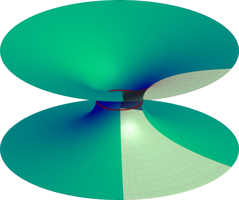
Figure 1. The catenoid surface with the “collar” (thinnest part of the surface of revolution) marked out. In the transparent portion we can see the level sets of the angular coordinate $\omega$ as well as the “radial” coordinate $y$.

2. Main Results

2.1. Formulation of the problem

As mentioned above, we consider perturbations of the stationary catenoid solution to the extremal surface equation. The catenoid as a surface of revolution can be parametrized by (see also Figure 1)

$$\mathbb{R}\times\mathbb{S}^{1}\ni(y,\omega)\mapsto\left(r=\sqrt{1+y^{2}},z=\sinh^{-1}y,\theta=\omega\right)\in\mathbb{R}_{+}\times\mathbb{R}\times\mathbb{S}^{1},$$ (2.1)

where we use the standard cylindrical coordinates system on $\mathbb{R}^{3}$. Throughout we use the notation $\left\langle y\right\rangle=\sqrt{1+y^{2}}$. The parametrization here exposes the catenoid, a surface of revolution, as a warped product manifold with base $\mathbb{R}$ and fibre $\mathbb{S}$; the coordinate $y$ is chosen to be orthogonal to the fibers and to have unit length (note that the parametrization is “by arc length” if we “mod” out the rotational degree of freedom). In this coordinate system we see that the induced Riemannian metric on the catenoid has the line element

$$\mathrm{d}y^{2}+\left\langle y\right\rangle^{2}\mathrm{d}\omega^{2}~{},$$

and that $\left\langle y\right\rangle/\left|y\right|\to 1$ as $y\to\pm\infty$ captures the asymptotic flatness of this manifold.

In addition to the rotational symmetry, the catenoid also has a reflection symmetry about the plane $z=0$; in terms of the intrinsic coordinates, this is the mapping $y\mapsto-y$. For simplicity, we will consider only perturbations that preserve both symmetries. More precisely, we will consider the case where the perturbed solution is still, at any instance of time, a surface of revolution that is symmetric about the plane $z=0$. Note that since the induced Riemannian metric on $\Sigma$ is asymptotically flat with two ends, the Hamiltonian flow on $\mathbb{R}\times\Sigma$ using the pullback metric exhibits trapping, which is manifest in the closed geodesic at the “collar” of $\Sigma$ (see Figure 1). The rotational symmetry reduces our scenario to the “zero angular momentum case”, and hence issues associated with the trapping of the geodesic flow do not appear in our analysis. A treatment of the full problem, without rotational symmetry, will require a modification of some parts of our proof which rely explicitly on the 1+1 reduction of the problem in rotational symmetry, as well as a detailed study of the trapping phenomenon, which usually induces a loss of derivatives. On the other hand, the reflection symmetry is only used to simplify the analysis by effectively fixing the centre of mass; we do not expect there to be obstructions in removing this assumption given finite speed of propagation for nonlinear wave equations.

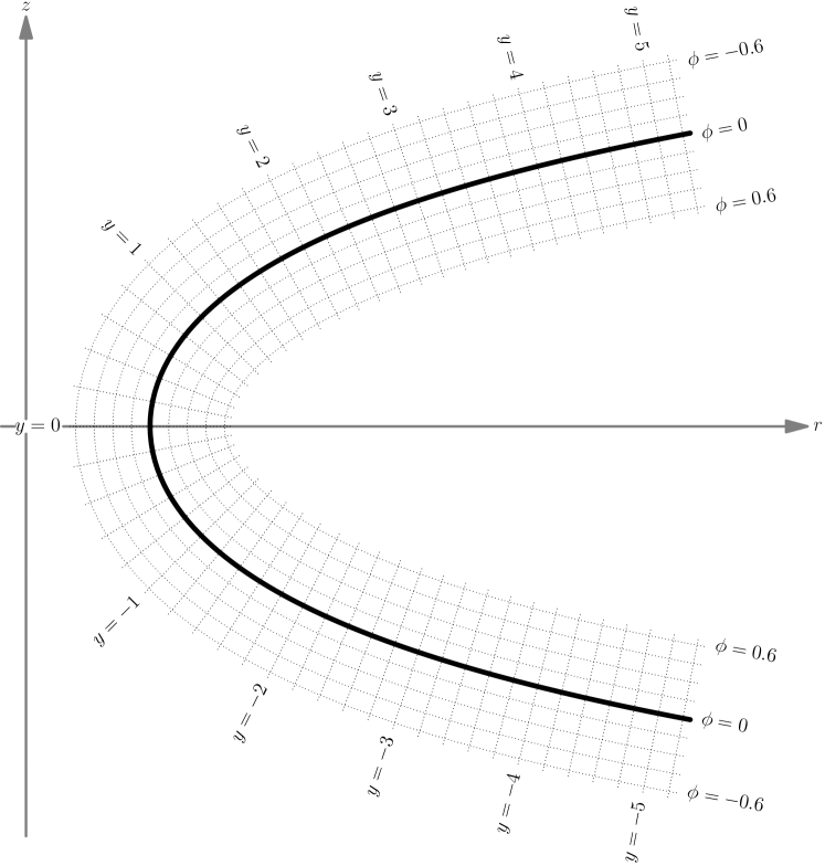
Figure 2. The local coordinate system induced by the normal bundle of the catenoid. We show here the cross section for a fixed $\omega$.

Given the geometric nature of our problem, there are many different ways of parametrizing our solution manifold $M$ (or equivalently, fixing the time parameter $t$, parametrizing the time slices). To cast the problem as a concrete system of partial differential equations requires choosing a gauge (in other words, fixing a preferred parametrization; this problem is typical for geometric equations such as the Ricci flow or Einstein equations). Given the assumed symmetries one may be tempted into a geometric gauge choice via intrinsic quantities: for example, the rotational symmetry means that naturally $\omega$ is a good candidate coordinate, and we may want to choose the other coordinate $y$ of $\Sigma$ to be orthogonal to $\omega$ and of unit length, similar to our parametrization of the catenoid. This choice turns out to be not suitable for studying the stability problem as the equation for the difference between our perturbed solution and the stationary catenoid becomes a complicated equation for a vector-valued function with a compatibility constraint (coming from the “unit-length” requirement). By using the compatibility constraint one can convert this to a scalar non-local integro-differential equation.

Since we are interested in the stability problem in the rotationally symmetric case, instead we will consider our perturbed solution as a graph over the catenoid. More precisely, using that the outward-pointing unit normal vector field to the catenoid is $\left\langle y\right\rangle^{-1}(\partial_{r}-y\partial_{z})$, there is a natural smooth surjection from the normal bundle of the catenoid to $\mathbb{R}^{3}$, given by (see Figure 2)

$$(y,\omega,\phi)\mapsto\left(r=\left\langle y\right\rangle+\frac{\phi}{\left\langle y\right\rangle},z=\sinh^{-1}y-\frac{y\phi}{\left\langle y\right\rangle},\theta=\omega\right)~{}.$$ (2.2)

By considering the radius of curvature for the constant $\omega$ level curves, we see that restricted to $\left|\phi\right|<\left\langle y\right\rangle^{2}$ this mapping is regular and injective. Since we are interested in perturbations of the $\phi=0$ level set, we make the assumption that our perturbed solution can be written as a graph over $\{\phi=0\}$ in this coordinate system. That is to say, we will study the small data problem for $\phi=\phi(t,y)$. Note that our assumption of reflection symmetry implies that $\phi$ will be an even function in $y$, and the lack of $\omega$ dependence indicates that the graph is a surface of revolution.

Under this parametrization, we can derive the equation of motion for the extremal surface by formally writing down the Euler-Lagrange equations for the Lagrangian given by the induced volume form on the graph associated to $\phi(t,y)$; this computation is carried out in Appendix A. We find that the equation of motion can be written as a quasilinear wave equation with potential for $\phi$ in the coordinates $t,y$:

$$-\partial_{tt}^{2}\phi+\partial_{yy}^{2}\phi+\frac{y}{\left\langle y\right\rangle^{2}}\partial_{y}\phi+\frac{2}{\left\langle y\right\rangle^{4}}\phi=Q_{2}+Q_{3}+Q_{4}+S_{2}+S_{3}+S_{4},$$ (2.3)

where the quasilinear terms $Q_{*}$ and semilinear terms $S_{*}$ are split into those quadratic, cubic, and quartic-or-more in $\phi$ and its derivatives:

$$Q_{2} =-\frac{2\phi}{\left\langle y\right\rangle^{2}}\partial^{2}_{tt}\phi,$$ (2.4a)

$$Q_{3} =\frac{\phi^{2}}{\left\langle y\right\rangle^{4}}\partial^{2}_{yy}\phi+(\partial_{t}\phi)^{2}\partial^{2}_{yy}\phi-2\partial_{t}\phi\partial_{y}\phi\partial^{2}_{ty}\phi+(\partial_{y}\phi)^{2}\partial^{2}_{tt}\phi,$$ (2.4b)

$$Q_{4} =\frac{\phi^{2}}{\left\langle y\right\rangle^{4}}\left[\left(\frac{2\phi}{\left\langle y\right\rangle^{2}}-\frac{\phi^{2}}{\left\langle y\right\rangle^{4}}-(\partial_{y}\phi)^{2}\right)\partial^{2}_{tt}\phi+2\partial_{y}\phi\partial_{t}\phi\partial^{2}_{ty}\phi-(\partial_{t}\phi)^{2}\partial^{2}_{yy}\phi\right],$$ (2.4c)

and

$$S_{2} =\frac{4\phi^{2}}{\left\langle y\right\rangle^{6}}+\frac{4y\phi\partial_{y}\phi}{\left\langle y\right\rangle^{4}}-\frac{(\partial_{y}\phi)^{2}}{\left\langle y\right\rangle^{2}},$$ (2.5a)

$$S_{3} =\frac{y\phi^{2}}{\left\langle y\right\rangle^{6}}\partial_{y}\phi-\frac{2\phi^{3}}{\left\langle y\right\rangle^{8}}-\left(\frac{3\phi}{\left\langle y\right\rangle^{4}}+\frac{y\partial_{y}\phi}{\left\langle y\right\rangle^{2}}\right)(\partial_{y}\phi)^{2}+\left(\frac{2\phi}{\left\langle y\right\rangle^{4}}+\frac{y\partial_{y}\phi}{\left\langle y\right\rangle^{2}}\right)(\partial_{t}\phi)^{2},$$ (2.5b)

$$S_{4} =-\left(\frac{4y\phi}{\left\langle y\right\rangle^{4}}+\frac{y\phi^{2}}{\left\langle y\right\rangle^{6}}\right)\partial_{y}\phi(\partial_{t}\phi)^{2}-\left(\frac{4\phi^{2}}{\left\langle y\right\rangle^{6}}-\frac{2\phi^{3}}{\left\langle y\right\rangle^{8}}\right)(\partial_{t}\phi)^{2}.$$ (2.5c)

We denote by $F$ this nonlinearity

$$F(y,\phi,\nabla\phi,\nabla^{2}\phi)=Q_{2}+Q_{3}+Q_{4}+S_{2}+S_{3}+S_{4}~{}.$$ (2.6)

2.2. A first look at the structure of the equation

Let us point out some of the main features of the equations (2.3), (2.4), and (2.5). That our argument can control the nonlinear terms using pointwise decay estimates is largely due to two special structures: the terms are either localized or they exhibit a null condition. We comment on these structures in Section 2.2.1. The linear evolution introduces additional difficulties as there is an exponentially growing mode: the pointwise decay estimates we need can only be expected away from the growing mode. This is discussed in Section 2.2.2.

2.2.1. Nonlinearities

The reason that we separated the quadratic, cubic, and quartic-and-higher nonlinearities is that we intend to make use of the radiative decay effects of the wave equation on a (2+1) dimensional, asymptotically flat space-time to gain decay in the “wave zone”, the region where $y$ and $t$ are comparable. The experience with small-data, quasilinear wave equations on $\mathbb{R}^{1,2}$, see [20, 1, 2], indicates that the most dangerous terms are those which are quadratic and cubic in the nonlinearities, due to the expected linear decay rate of $1/\sqrt{t}$ for wave equations in 2 spatial dimensions (see also Section 2.3).

On the other hand, in (2.4) and (2.5), almost all the nonlinear terms, in particular all the quadratic ones, gain an additional boost in decay from the coefficients of the form $\left\langle y\right\rangle^{-k}$ — in the wave zone this term contributes a decay rate of $t^{-k}$ which vastly improves the situation. The term $Q_{2}$, for example, has the form $O(t^{-5/2})\cdot\partial^{2}_{tt}\phi$ with a coefficient which is much better than the integrability threshold of $O(t^{-1})$, if we assume an expected linear decay rate. As we shall see in the analysis, this localization of some of the most dangerous nonlinearities plays a crucial role in allowing us to close our decay estimates.

The only exception to this boost in decay occurs in the term $Q_{3}$: there we have a non-linearity of the form

$$(\partial_{t}\phi)^{2}\partial^{2}_{yy}\phi-2\partial_{t}\phi\partial_{y}\phi\partial^{2}_{ty}\phi+(\partial_{y}\phi)^{2}\partial^{2}_{tt}\phi~{}$$ (2.7)

which is unweighted. However, as was observed in [20] for the perturbation of the trivial solution, this term carries a null structure. One can see this purely at an algebraic level: in terms of the background null coordinates $u=t+y$ and $v=t-y$, the nonlinearity takes the form

$$4(\partial_{v}\phi)^{2}\partial^{2}_{uu}\phi+4(\partial_{u}\phi)^{2}\partial^{2}_{vv}\phi-8\partial_{u}\phi\partial_{v}\phi\partial^{2}_{uv}\phi$$

and hence verifies the cubic, quasilinear null condition [1]. The null condition exhibits in particular a hidden divergence/gradient structure: in the context of elliptic theory it appears in the proof of Wente’s inequality [29]; and in the context of wave equations it drives the null form estimates of Klainerman and Machedon [16]. For our explicit nonlinearity above, one can check easily that the following identity holds

$$(\partial_{t}\phi)^{2}\partial^{2}_{yy}\phi-2\partial_{t}\phi\partial_{y}\phi\partial^{2}_{ty}\phi+(\partial_{y}\phi)^{2}\partial^{2}_{tt}\phi\\ =\partial_{t}\big{[}(\partial_{t}\phi)^{3}\big{]}-2\partial_{y}\big{[}\partial_{y}\phi(\partial_{t}\phi)^{2}\big{]}+\partial_{t}\big{[}(\partial_{y}\phi)^{2}\partial_{t}\phi\big{]}+3(\partial_{t}\phi)^{2}(\partial^{2}_{yy}\phi-\partial^{2}_{tt}\phi).$$

The first three terms of the right-hand side exhibit the hidden divergence structure, while for the last term, we may replace $-\partial^{2}_{tt}\phi+\partial^{2}_{yy}\phi$ using our original equation (2.3) and hence obtain terms which are cubic with sufficient weights together with quartic and higher terms which have better decay properties.

2.2.2. Linear spectral analysis

Having described the difficulties that arise from the “right hand side” of (2.3), we turn our attention to the “left hand side”. The linear operator

$$-\partial^{2}_{tt}\phi+\partial^{2}_{yy}\phi+\frac{y}{\left\langle y\right\rangle^{2}}\partial_{y}\phi$$ (2.8)

is in fact the coordinate-invariant wave operator $\Box_{M}\phi$ on the background $\mathbb{R}\times\Sigma$. Indeed, the induced Lorentzian metric on the stationary catenoid solution, as an embedded hypersurface of $\mathbb{R}^{1,3}$, is

$$-\mathrm{d}t^{2}+\mathrm{d}y^{2}+\left\langle y\right\rangle^{2}\mathrm{d}\omega^{2}~{},$$

and its corresponding Laplace-Beltrami operator can be computed to be exactly (2.8). However, since we are considering the perturbation of a non trivial solution, there is also a lower order correction term generated by the linearization, namely the potential term $2\left\langle y\right\rangle^{-4}\phi$ on the left hand side of (2.3). Note that the coefficient $2\left\langle y\right\rangle^{-4}$ has a positive sign, which indicates that it is an attractive potential, and opens up the possibility of the existence of a negative energy ground state. This is related to the variational instability of the catenoid as a minimal surface [12]: indeed, geometrically we can write the linear operator on the left hand side of (2.3) as

$$\Box_{g}-\mathrm{Scalar}$$

where $\Box_{g}$ is the Laplace-Beltrami operator for the induced Lorentzian metric on the static catenoid solution, and $\mathrm{Scalar}$ is the induced scalar curvature. This operator is formally the second variation of the extremal surface Lagrangian, and in the Riemannian case is precisely the stability operator for minimal hypersurfaces embedded in Euclidean spaces. The positivity of the potential term and the linear instability is then seen as a consequence of minimal surfaces in $\mathbb{R}^{3}$ necessarily having negative Gaussian curvature. Any corresponding eigenfunction of the linearized operator will generate either non-decaying or exponentially growing modes; clearly this will complicate our estimates based on expectation of linear pointwise decay.

Now, the natural space on which to study our linear operator is the $L^{2}$ space adapted to the geometry; that is to say, we should be looking at $L^{2}(\Sigma)$ where $\Sigma$ is the catenoid. In the intrinsic coordinates $(y,\omega)$ this is $L^{2}(\left\langle y\right\rangle\mathrm{d}y\,\mathrm{d}\omega)$. Since we are working with rotationally symmetric functions, we find it convenient to absorb the weight $\left\langle y\right\rangle$ onto the function $\phi$ instead, and work with $L^{2}(\mathrm{d}y)$. In other words we introduce the notation

$$\tilde{\phi}:=\left\langle y\right\rangle^{\frac{1}{2}}\phi$$

and we obtain in place of (2.3) the following equation:

$$-\partial_{t}^{2}\tilde{\phi}+\partial_{y}^{2}\tilde{\phi}+\frac{6+y^{2}}{4\left\langle y\right\rangle^{4}}\tilde{\phi}=\left\langle y\right\rangle^{\frac{1}{2}}F(\phi,\nabla\phi,\nabla^{2}\phi).$$ (2.9)

Thus, we are now working with the standard $L^{2}(\mathrm{d}y)$ space and on this space the relevant linear operator

$$\mathcal{L}:=-\partial_{y}^{2}-\frac{6+y^{2}}{4\left\langle y\right\rangle^{4}}$$ (2.10)

is a short-range perturbation of the Laplacian. Since the potential term is a bounded multiplier which decays to $0$ as $\left|y\right|\to\infty$, the operator $\mathcal{L}$ is self-adjoint on $L^{2}(\mathrm{d}y)$ with domain $\{\partial^{2}_{yy}f\in L^{2}(\mathrm{d}y)\}$, and its essential spectrum is exactly $[0,\infty)$ (this result is classical, see e.g. [14, Sections 13.1 and 14.3]). Due to the $O(\left\langle y\right\rangle^{-2})$ decay of the potential term, the solutions to the ordinary differential equation $(\mathcal{L}-\lambda)\eta_{\lambda}=0$ for $\lambda>0$ are given by the Jost solutions [27, Theorem XI.57], and hence there are no $L^{2}$ eigenfunctions with positive eigenvalue.

In the case $\lambda=0$, the equation $\mathcal{L}\eta_{0}=0$ can be solved explicitly: this is simply due to the fact that $\mathcal{L}$ is the natural linearized operator for the minimal surface embedding problem, and that after fixing rotational symmetry, the catenoid solutions form a two parameter family due to the freedoms for scaling and translating (along the axis). To be more precise, the standard catenoid we choose in (2.1) is the element of the family

$$(y,\omega)\mapsto\left(r=a\left\langle a^{-1}y\right\rangle,z=b+a\sinh^{-1}(a^{-1}y),\theta=\omega\right)~{},$$ (2.11)

parametrized by $(a,b)\in\mathbb{R}_{+}\times\mathbb{R}$, with $a=1$ and $b=0$. The two linearly independent solutions to $\mathcal{L}\eta_{0}=0$ correspond to infinitesimal motions in $a$ and $b$ of the above. From this consideration it is clear that the movement in $b$ corresponds to an odd solution (and so ruled out by our symmetry assumptions) with a unique root at $y=0$, while movement in $a$ corresponds to an even solution with two roots. We can easily obtain the explicit form of these two solutions by formally taking derivatives relative to $a,b$ after expressing (2.11) in the coordinates (2.2). This yields

$$\eta_{0}=\left\langle y\right\rangle^{\frac{1}{2}}\cdot\begin{cases}\frac{y}{\left\langle y\right\rangle}\sinh^{-1}y-1&\text{(scaling symmetry in }a),\\ \frac{y}{\left\langle y\right\rangle}&\text{(translation symmetry in }b).\end{cases}$$ (2.12)

One sees easily from the asymptotic behavior that neither of these functions belong to $L^{2}(\mathrm{d}y)$.

Remark 2.1.

The fact that the solutions $\eta_{0}$ do not belong to $L^{2}(\mathrm{d}y)$ implies that we do not have to modulate. In other words, the individual elements of our two parameter family (2.11) are “infinitely far” from one another (this can be seen from their asymptotic behavior) and we do not need to track the “motion along the soliton manifold” for our analysis.

We lastly consider the possible discrete spectrum below 0. By testing with bump functions we easily see that there must be a negative eigenvalue. By the Sturm-Picone comparison theorem [7, Section 10.6] and the explicit solutions (2.12) above, we see that the eigenvalue is unique, and its eigenfunction is nowhere vanishing (it is the ground state). We call this eigenfunction $g_{d}(y)$ and its associated eigenvalue $-k_{d}^{2}$. (Numerically $\sim-0.5857$.) Note that $g_{d}$ is smooth, and decays exponentially as $\left|y\right|\to\infty$.

In the sequel we let $P_{d}$ denote the projection onto the ground state $g_{d}$, and $P_{c}$ the projection onto the continuous spectrum. Noting that $g_{d}$ contributes an exponentially growing mode to the linear evolution, we cannot expect to have stability for any perturbation. Instead, we will show that given a sufficiently small initial perturbation $\tilde{\phi}$, we can adjust its projection to the ground state $P_{d}\tilde{\phi}$ while keeping $P_{c}\tilde{\phi}$ unchanged so as to guarantee global existence and asymptotic vanishing of the solution. In the analysis we will treat the continuous part and the discrete part of the spectrum separately. We will describe the linear decay estimates for the continuous part of the solution in Section 2.3. This will be combined with the analysis of the nonlinear terms (in the spirit of Section 2.2.1) to derive a priori estimates assuming that the discrete part of the solution is well behaved. Finally we will close the argument in Section 7 by showing that such a good choice of initial $P_{d}\tilde{\phi}$ is possible.

2.3. Energy bounds and pointwise decay estimates for $\mathcal{L}$

For the sequel, we shall use the following key energy and decay estimates associated with the evolution of the operator $\mathcal{L}$, which are proved in [11]. Recall that we take $P_{c}=1-P_{d}$ to be the projection to the continuous part of the spectrum of $\mathcal{L}$. In the sequel, we shall frequently use the notations (as well as variations thereof)

$$\|\langle\nabla_{t,y}\rangle^{\alpha}\psi\|_{S},\,\,\|\langle\nabla_{t,y}\rangle^{\alpha}\langle\Gamma\rangle^{\kappa}\psi\|_{S}$$

for various norms $\|\cdot\|_{S}$. By these expressions we shall understand the quantities

$$\sum_{0\leq|\beta|\leq\alpha}\|\nabla_{t,y}^{\beta}\psi\|_{S},\,\,\,\sum_{0\leq|\beta|\leq\alpha}\sum_{0\leq\tilde{\kappa}\leq\kappa}\|\nabla_{t,y}^{\beta}\Gamma^{\tilde{\kappa}}\psi\|_{S}.$$

Here $\Gamma$ stands for either one of the vector fields $\Gamma_{1}=t\partial_{y}+y\partial_{t}$, $\Gamma_{2}=t\partial_{t}+y\partial_{y}$.

Proposition 2.1.

For any multi-index $\alpha=(\alpha_{1},\alpha_{2})\in\mathbb{N}_{\geq 0}^{2}$, we have

$$\|\nabla_{t,y}^{\alpha}P_{c}e^{it\sqrt{\mathcal{L}}}f\|_{L^{2}_{dy}}\lesssim\|\langle\partial_{y}\rangle^{|\alpha|}f\|_{L^{2}_{dy}}$$ (2.13)

with constant depending on $|\alpha|=\alpha_{1}+\alpha_{2}$. Moreover, denoting the scaling vector field

$$\Gamma_{2}:=t\partial_{t}+y\partial_{y},$$

we have for any $\alpha\in\mathbb{N}_{\geq 0}$, $\beta\in\mathbb{N}_{\geq 0}^{2}$ the weighted energy bounds

$$\|\nabla_{t,y}^{\beta}\Gamma_{2}^{\alpha}P_{c}e^{it\sqrt{\mathcal{L}}}f\|_{L^{2}_{dy}}\lesssim\|\langle y\rangle^{\alpha}\langle\partial_{y}\rangle^{|\beta|+\alpha}f\|_{L^{2}_{dy}}.$$ (2.14)

For the sine evolution, we have the following bounds for $|\alpha|\geq 1$: for any $\varepsilon_{*}\geq 0$

$$\|\nabla_{t,y}^{\alpha}P_{c}\frac{\sin(t\sqrt{\mathcal{L}})}{\sqrt{\mathcal{L}}}f\|_{L^{2}_{dy}}\lesssim\|\langle\partial_{y}\rangle^{|\alpha|-1}f\|_{L^{2}_{dy}}+\|f\|_{L^{1}_{\langle y\rangle^{\varepsilon_{*}}dy}}$$ (2.15)

as well as

$$\|\nabla_{t,y}^{\alpha}\Gamma_{2}^{\kappa}P_{c}\frac{\sin(t\sqrt{\mathcal{L}})}{\sqrt{\mathcal{L}}}f\|_{L^{2}_{dy}}\lesssim\|\langle\partial_{y}\rangle^{|\alpha|-1}\langle\Gamma_{2}\rangle^{\kappa}f\|_{L^{2}_{dy}}+\|\langle\Gamma_{2}\rangle^{\kappa}f\|_{L^{1}_{\langle y\rangle^{\varepsilon_{*}}dy}}.$$ (2.16)

As for radiative decay, we have the following: for every $\sigma\in[1/2,1]$, it holds that

$$\|\langle y\rangle^{-\sigma}P_{c}e^{it\sqrt{\mathcal{L}}}f\|_{L^{\infty}_{dy}}\lesssim\langle t\rangle^{-\sigma}\big{[}\|\langle y\rangle^{\sigma}f\|_{L^{1}_{dy}}+\|\langle y\rangle^{\sigma}f^{\prime}\|_{L^{1}_{dy}}\big{]},$$

and

$$\|\langle y\rangle^{-\sigma}P_{c}\frac{\sin(t\sqrt{\mathcal{L}})}{\sqrt{\mathcal{L}}}g\|_{L^{\infty}_{dy}}\lesssim\langle t\rangle^{-\sigma}\|\langle y\rangle^{\sigma}g\|_{L^{1}_{dy}}.$$

Remark 2.2.

In [11], the linear estimates (2.15) and (2.16) are proven with $\varepsilon_{*}=0$, which imply the stated versions above. We introduce the $\left\langle y\right\rangle^{\varepsilon_{*}}$ weight (which should be regarded as a constraint on the decay rate of initial data) in order to prevent logarithmic divergences when controlling the nonlinear contributions. As such, $\varepsilon_{*}$ should be considered a small positive number that is fixed once and for all.

Remark 2.3.

For the radiative decay, the value $\sigma=\frac{1}{2}$ corresponds to the natural, unweighted decay for wave equations on $1+2$ dimensional space-times. The values $\sigma>\frac{1}{2}$ are weighted estimates factoring in spatial localizations.

The preceding bounds are still too crude to handle the unweighted cubic interaction terms that shows up in $Q_{3}$ of (2.4), and so we complement them with the following.

Proposition 2.2.

For any multi-index $\alpha=(\alpha_{1},\alpha_{2})\in\mathbb{N}_{\geq 0}^{2}$, $|\alpha|\geq 1$, we have

$$\|\nabla_{t,y}^{\alpha}P_{c}\frac{\sin(t\sqrt{\mathcal{L}})}{\sqrt{\mathcal{L}}}(\partial_{y}f)\|_{L^{2}_{dy}}\lesssim\|\langle\partial_{y}\rangle^{|\alpha|}f\|_{L^{2}_{dy}},$$ (2.17)

$$\|\nabla_{t,y}^{\alpha}\Gamma_{2}^{\kappa}P_{c}\frac{\sin(t\sqrt{\mathcal{L}})}{\sqrt{\mathcal{L}}}(\partial_{y}f)\|_{L^{2}_{dy}}\lesssim\|\langle\partial_{y}\rangle^{|\alpha|}\langle\Gamma_{2}\rangle^{\kappa}f\|_{L^{2}_{dy}},$$ (2.18)

as well as for the inhomogeneous evolution

$$\|\nabla_{t,y}^{\alpha}P_{c}\int_{0}^{t}\frac{\sin\left((t-s)\sqrt{\mathcal{L}}\right)}{\sqrt{\mathcal{L}}}(\partial_{s}F)\|_{L^{2}_{dy}}\lesssim\|\langle\nabla_{s,y}\rangle^{|\alpha|}F\|_{L_{s}^{1}L^{2}_{dy}},$$ (2.19)

$$\|\nabla_{t,y}^{\alpha}\Gamma_{2}^{\kappa}P_{c}\int_{0}^{t}\frac{\sin\left((t-s)\sqrt{\mathcal{L}}\right)}{\sqrt{\mathcal{L}}}(\partial_{s}F)\|_{L^{2}_{dy}}\lesssim\|\langle\nabla_{s,y}\rangle^{|\alpha|}\langle\Gamma_{2}\rangle^{\kappa}F\|_{L_{s}^{1}L^{2}_{dy}}.$$ (2.20)

In order to handle the local terms in (2.3), we need a local energy decay result. This is given by the following

Proposition 2.3.

We have the space-time bounds

$$\|\langle y\rangle^{-1}\nabla_{t,y}^{\alpha}\Gamma_{2}^{\kappa}\cos(t\sqrt{\mathcal{L}})P_{c}f\|_{L^{2}_{t,y}}+\|\langle y\log y\rangle^{-1}\nabla_{t,y}^{\alpha}\Gamma_{2}^{\kappa}\frac{\sin(t\sqrt{\mathcal{L}})}{\sqrt{\mathcal{L}}}P_{c}g\|_{L_{t,y}^{2}}$$

$$\lesssim\|\langle\partial_{y}\rangle^{|\alpha|}\langle\Gamma\rangle^{\kappa}f\|_{L^{2}_{dy}}+\|\langle\partial_{y}\rangle^{|\alpha|-1}\langle\Gamma\rangle^{\kappa}g\|_{L^{2}_{\langle y\rangle^{1+}dy}}.$$

The inhomogeneous version with source terms of gradient structure is as follows:

$$\|\langle y\log y\rangle^{-1}\nabla_{t,y}^{\alpha}\Gamma_{2}^{\kappa}P_{c}\int_{0}^{t}\frac{\sin(t-s)\sqrt{\mathcal{L}})}{\sqrt{\mathcal{L}}}(\partial_{s,y}F)\|_{L^{2}_{t,y}}\lesssim\|\langle\nabla_{s,y}\rangle^{|\alpha|}\langle\Gamma_{2}\rangle^{\kappa}F\|_{L_{s}^{1}L^{2}_{dy}}.$$

These linear estimates were proven in [11] for a large class of $1+1$ dimensional wave equations with potentials. The main technique used there is that of the distorted Fourier transform, which is essentially the representation of solutions as superpositions of generalized eigenfunctions of the linear operator $\mathcal{L}$ (analogous to how the Fourier transform represents functions as superpositions of generalized eigenfunctions of the Laplacian). When restricted to the continuous part of the spectrum, this representation allows the use of oscillatory integral techniques to obtain dispersive estimates. Part of the difficulty in implementing this process is in analyzing the spectral measure and obtain suitable descriptions of the generalized eigenfunctions. These are done in detail in [11].

To control the decay rate of the nonlinear evolution, in addition to the standard dispersive bounds we also need a variation of the vector field method to take advantage of the algebraic structure of the nonlinearities. Recall that the vectorfields associated to $-\partial^{2}_{t}+\partial^{2}_{y}$ are the Lorentz boost generator $\Gamma_{1}=t\partial_{y}+y\partial_{t}$ and the generator of scaling symmetry $\Gamma_{2}=t\partial_{t}+y\partial_{y}$. In our problem, we cannot obtain estimates on $\Gamma\phi$ using the estimates available for solutions $\phi$, since $\Gamma_{1,2}$ do not commute with the linearized operator $\mathcal{L}$. To overcome this in [11] a method is introduced where bounds on $\Gamma_{2}$ are obtained by studying its analogue under the distorted Fourier transform. From these linear estimates on $\Gamma_{2}$ derivatives we obtain control on $\Gamma_{1}$ derivatives, by using the structure of the equation and the behavior of the solution in the space-time regions $y\ll t$ and $y\gtrsim t$; see Lemma 4.1 for details.

2.4. Main Theorem

The unstable mode associated with $\mathcal{L}$ should lead in general to exponentially growing solutions for (2.9), even for arbitrarily small initial data. Nonetheless, it is natural to expect the existence of a suitable co-dimension one set of small initial data corresponding to solutions which exist globally in forward time and decay toward zero, i. e. the evolved surface converges to the static catenoid. This is proved in the following theorem which is our main result.

Theorem 2.4 (Codimension one stability of the catenoid).

Let us be given a pair of even functions $(\tilde{\phi}_{1},\tilde{\phi}_{2})\in W^{N_{0},1}(\mathbb{R})\cap W^{N_{0},2}(\mathbb{R})$ satisfying the smallness condition

$$\|\tilde{\phi}\|_{X_{0}}:=\sum_{j=1,2}\|\langle y\rangle^{N_{0}-j+1}\langle\partial_{y}\rangle^{N_{0}-j+1}\tilde{\phi}_{j}\|_{L^{1}_{dy}\cap L^{2}_{dy}}\leq\delta_{0}$$

for $\delta_{0}>0$ sufficiently small, and $N_{0}$ sufficiently large. Then there exists a parameter $a\in\mathbb{R}$ which depends Lipschitz continuously on $\tilde{\phi}_{1,2}$ with respect to $X_{0}$ such that the solution $\tilde{\phi}$ of (2.9) corresponding to the initial data

$$\left(\tilde{\phi}(0,\cdot),\partial_{t}\tilde{\phi}(0,\cdot)\right)=(\tilde{\phi}_{1}+ag_{d},\tilde{\phi}_{2})$$

exists globally in forward time $t>0$. Moreover, $\phi=\langle y\rangle^{-1/2}\tilde{\phi}$ decays toward zero:

$$|\phi(t,\cdot)|\lesssim\langle t\rangle^{-\frac{1}{2}}.$$

An interesting open problem is the description of the flow in the neighborhood of the codimension 1 manifold of Theorem 2.4, and in particular whether this manifold is a threshold between two different types of stable regimes. An analogous problem has been studied in [21] in the case of the $L^{2}$ critical nonlinear Schrödinger equation. The initial data corresponding to Bourgain-Wang solutions (which are expected to form a co-dimension one manifold [19]), are shown to lie at the boundary between solutions blowing up in finite time in the log-log regime and solutions scattering to 0 (note that both are known to be stable regimes for that equation). Numerical simulations for the extremal surface equation suggest that a similar behavior might take place here. Indeed, the codimension 1 manifold of Theorem 2.4 seems to be the threshold between two types of regimes: one leading to a collapse of the collar ($\phi\to-\left\langle y\right\rangle^{2}$ for some $\left|y\right|\ll 1$ and the solution ceases to be an immersed submanifold), and another leading to the accelerated widening of the collar region.

3. Setting up the analysis

The aim of this section is to set up the bootstrap argument.

3.1. Spectral decomposition of the solution

We decompose our solution $\tilde{\phi}$ as

$$\tilde{\phi}=h(t)g_{d}+\tilde{\psi}$$

so that $\tilde{\psi}$ satisfies

$$\langle\tilde{\psi},g_{d}\rangle=0.$$

Thus, we have

$$P_{d}\tilde{\phi}=h(t)g_{d},\,\,P_{c}\tilde{\phi}=\tilde{\psi}.$$

In particular, $\tilde{\psi}$ satisfies in view of (2.9)

$$\begin{cases}-\partial_{t}^{2}\tilde{\psi}+\partial_{y}^{2}\tilde{\psi}+\frac{1}{2}\frac{3+\frac{y^{2}}{2}}{(1+y^{2})^{2}}\tilde{\psi}=P_{c}((1+y^{2})^{\frac{1}{4}}F(y,\phi,\nabla\phi,\nabla^{2}\phi)),\\ \tilde{\psi}(0,.)=P_{c}\tilde{\phi}_{1},\,\,\partial_{t}\tilde{\psi}(0,.)=P_{c}\tilde{\phi}_{2}.\end{cases}$$ (3.1)

We derive a formula for $h(t)$ in the following lemma.

Lemma 3.1.

$h(t)$ is given by

$$h(t)$$

$$= \frac{1}{2}\left(a+\langle\tilde{\phi}_{1},g_{d}\rangle+\frac{\langle\tilde{\phi}_{2},g_{d}\rangle}{k_{d}}-\frac{1}{k_{d}}\int_{0}^{t}\langle(1+y^{2})^{\frac{1}{4}}F(\phi,\nabla\phi,\nabla^{2}\phi)(s),g_{d}\rangle e^{-k_{d}s}ds\right)e^{k_{d}t}$$

$$+ \frac{1}{2}\left(a+\langle\tilde{\phi}_{1},g_{d}\rangle-\frac{\langle\tilde{\phi}_{2},g_{d}\rangle}{k_{d}}+\frac{1}{k_{d}}\int_{0}^{t}\langle(1+y^{2})^{\frac{1}{4}}F(\phi,\nabla\phi,\nabla^{2}\phi)(s),g_{d}\rangle e^{k_{d}s}ds\right)e^{-k_{d}t}.$$

Proof.

$h(t)$ satisfies in view of (2.9) and the fact that $g_{d}$ is en eigenvector of $\mathcal{L}$ with eigenvalue $-k_{d}^{2}$:

$$-h^{\prime\prime}(t)+k_{d}^{2}h(t)=\langle(1+y^{2})^{\frac{1}{4}}F(\phi,\nabla\phi,\nabla^{2}\phi),g_{d}\rangle.$$

Using the variation of constant methods, we deduce

$$h(t) = \left(A_{1}-\frac{1}{2k_{d}}\int_{0}^{t}\langle(1+y^{2})^{\frac{1}{4}}F(\phi,\nabla\phi,\nabla^{2}\phi)(s),g_{d}\rangle e^{-k_{d}s}ds\right)e^{k_{d}t}$$

$$+\left(A_{2}+\frac{1}{2k_{d}}\int_{0}^{t}\langle(1+y^{2})^{\frac{1}{4}}F(\phi,\nabla\phi,\nabla^{2}\phi)(s),g_{d}\rangle e^{k_{d}s}ds\right)e^{-k_{d}t}.$$

Since we have

$$h(0)=a+\langle\tilde{\phi}_{1},g_{d}\rangle,\,\,h^{\prime}(0)=\langle\tilde{\phi}_{2},g_{d}\rangle,$$

we deduce

$$A_{1}=\frac{1}{2}\left(a+\langle\tilde{\phi}_{1},g_{d}\rangle+\frac{\langle\tilde{\phi}_{2},g_{d}\rangle}{k_{d}}\right)\textrm{ and }A_{2}=\frac{1}{2}\left(a+\langle\tilde{\phi}_{1},g_{d}\rangle-\frac{\langle\tilde{\phi}_{2},g_{d}\rangle}{k_{d}}\right).$$

This concludes the proof of the lemma. ∎

3.2. Setting up the bootstrap

Consider a time $T>0$ such that the following bootstrap assumptions hold on $[0,T)$:

$$\|\nabla_{t,y}\nabla_{t,y}^{\alpha}\tilde{\phi}\|_{L^{2}_{dy}}\leq\varepsilon\langle t\rangle^{\nu},\,0\leq|\alpha|\leq N_{1},$$ (3.2)

$$\|\nabla_{t,y}^{\beta}\phi\|_{L^{\infty}_{dy}}\leq\varepsilon\langle t\rangle^{-\frac{1}{2}},\,0\leq|\beta|\leq\frac{N_{1}}{2}+C,$$ (3.3)

$$\|\langle y\rangle^{-\frac{1}{2}}\nabla_{t,y}^{\beta}\phi\|_{L^{\infty}_{dy}}\leq\varepsilon\langle t\rangle^{-\frac{1}{2}-\delta_{1}},\,0\leq|\beta|\leq\frac{N_{1}}{2}+C,$$ (3.4)

$$\|\nabla_{t,y}\nabla_{t,y}^{\beta}\Gamma_{2}^{\gamma}\tilde{\phi}\|_{L^{2}_{dy}}\leq\varepsilon\langle t\rangle^{([\frac{2|\beta|}{N_{1}}]+1)10^{\gamma}\nu},\,0\leq|\beta|\leq N_{1}-\gamma,\,0\leq\gamma\leq 2,$$ (3.5)

$$\begin{split}&\|\langle y\log y\rangle^{-1}\big{(}\nabla_{t,y}^{\beta}\Gamma_{2}^{\gamma}\tilde{\phi})\|_{L^{2}_{t,y}([0,T])}\leq\varepsilon\langle T\rangle^{(\chi_{\gamma>0}[\frac{2|\beta|}{N_{1}}]+1)10^{\gamma}\nu},\\ &\hskip 170.71652pt0\leq|\beta|\leq 1+N_{1}-\gamma,\,0\leq\gamma\leq 2,\end{split}$$ (3.6)

$$\begin{split}&\sum_{\beta\leq N_{1}+1}|\partial_{t}^{\beta}h(t)|\leq\varepsilon\langle t\rangle^{-1-2\delta_{1}},\\ &\sum_{\beta+\kappa\leq N_{1}+1}|\partial_{t}^{\beta}(t\partial_{t})^{\kappa}h(t)|\leq\varepsilon\langle t\rangle^{(1+[\frac{2|\beta|}{N_{1}}])10^{\kappa}\nu},\,\kappa\in\{1,2\},\\ &\sum_{\beta+\kappa\leq N_{1}+1}\big{\|}\partial_{t}^{\beta}(t\partial_{t})^{\kappa}h\big{\|}_{L^{2}_{[0,T]}}\leq\varepsilon\langle T\rangle^{(1+[\frac{2|\beta|}{N_{1}}])10^{\kappa}\nu},\,\kappa\in\{1,2\}.\\ \end{split}$$ (3.7)

Our claim is that the above regime is trapped.

Proposition 3.2 (Improvement of the bootstrap assumptions).

There exists an $N_{1}$ sufficiently large, such that the following holds: there is $N_{0}$ sufficiently large, such that if $N_{1}\gg C\geq 10$ and given $\varepsilon>0$, $1\gg\delta_{1}\gg\nu\gg\varepsilon$, there is $\delta_{0}=\delta_{0}(\varepsilon,N_{0})>0$ sufficiently small (as in Theorem 2.4) and

$$a\in[-\varepsilon^{\frac{3}{2}},\,\varepsilon^{\frac{3}{2}}]$$

such that $\tilde{\phi}$ satisfies the following bounds

$$\|\nabla_{t,y}\nabla_{t,y}^{\alpha}\tilde{\phi}\|_{L^{2}_{dy}}\lesssim(\delta_{0}+\varepsilon^{\frac{3}{2}})\langle t\rangle^{\nu},\,0\leq|\alpha|\leq N_{1},$$ (3.8)

$$\|\nabla_{t,y}^{\beta}\phi\|_{L^{\infty}_{dy}}\lesssim(\delta_{0}+\varepsilon^{\frac{3}{2}})\langle t\rangle^{-\frac{1}{2}},\,0\leq|\beta|\leq\frac{N_{1}}{2}+C,$$ (3.9)

$$\|\langle y\rangle^{-\frac{1}{2}}\nabla_{t,y}^{\beta}\phi\|_{L^{\infty}_{dy}}\lesssim(\delta_{0}+\varepsilon^{\frac{3}{2}})\langle t\rangle^{-\frac{1}{2}-\delta_{1}},\,0\leq|\beta|\leq\frac{N_{1}}{2}+C,$$ (3.10)

$$\|\nabla_{t,y}\nabla_{t,y}^{\beta}\Gamma_{2}^{\gamma}\tilde{\phi}\|_{L^{2}_{dy}}\lesssim(\delta_{0}+\varepsilon^{\frac{3}{2}})\langle t\rangle^{([\frac{2|\beta|}{N_{1}}]+1)10^{\gamma}\nu},\,0\leq|\beta|\leq N_{1}-\gamma,\,0\leq\gamma\leq 2,$$ (3.11)

$$\begin{split}&\|\langle y\log y\rangle^{-1}\big{(}\nabla_{t,y}^{\beta}\Gamma_{2}^{\gamma}\tilde{\phi})\|_{L^{2}_{t,y}([0,T])}\lesssim(\delta_{0}+\varepsilon^{\frac{3}{2}})\langle T\rangle^{(\chi_{\gamma>0}[\frac{2|\beta|}{N_{1}}]+1)10^{\gamma}\nu},\\ &\hskip 170.71652pt0\leq|\beta|\leq 1+N_{1}-\gamma,\,0\leq\gamma\leq 2,\end{split}$$ (3.12)

$$\begin{split}&\sum_{\beta\leq N_{1}+1}|\partial_{t}^{\beta}h(t)|\lesssim(\delta_{0}+\varepsilon^{\frac{3}{2}})\langle t\rangle^{-1-2\delta_{1}},\\ &\sum_{\beta+\kappa\leq N_{1}+1}|\partial_{t}^{\beta}(t\partial_{t})^{\kappa}h(t)|\lesssim(\delta_{0}+\varepsilon^{\frac{3}{2}})\langle t\rangle^{(1+[\frac{2|\beta|}{N_{1}}])10^{\kappa}\nu},\,\kappa\in\{1,2\},\\ &\sum_{\beta+\kappa\leq N_{1}+1}\big{\|}\partial_{t}^{\beta}(t\partial_{t})^{\kappa}h\big{\|}_{L^{2}_{[0,T]}}\lesssim(\delta_{0}+\varepsilon^{\frac{3}{2}})\langle T\rangle^{(1+[\frac{2|\beta|}{N_{1}}])10^{\kappa}\nu},\,\kappa\in\{1,2\}.\\ \end{split}$$ (3.13)

The rest of the paper is as follows. In section 4, we prove the energy bounds (3.8) and (3.11). In section 5, we prove the local energy decay (3.12). In section 6, we prove the decay estimates (3.9) and (3.10). In section 7, we prove the existence of $a$ such that (3.13) holds which concludes the proof of Proposition 3.2. Finally, we prove Theorem 2.4 in section 8.

4. Energy bounds

The goal of this section is to prove the estimates (3.8) and (3.11).

4.1. The proof of the estimate (3.8)

In view of (3.1), we have

$$\tilde{\psi}=\cos(t\sqrt{\mathcal{L}})P_{c}\tilde{\phi}_{1}+\frac{\sin(t\sqrt{\mathcal{L}})}{\sqrt{\mathcal{L}}}P_{c}\tilde{\phi}_{2}+\int_{0}^{t}\frac{\sin([t-s]\sqrt{\mathcal{L}})}{\sqrt{\mathcal{L}}}P_{c}\big{(}G(s,\cdot)\big{)}\,ds$$ (4.1)

where

$$G(s,y)=(1+y^{2})^{\frac{1}{4}}F(y,\phi,\nabla\phi,\nabla^{2}\phi).$$

In order to derive the desired energy bounds, we can use Proposition 2.1 for the weighted terms without maximum order derivatives, and Proposition 2.2 for the pure cubic terms, as we shall see. In order to deal with the maximum order derivative terms, we have to use a direct integration by parts argument. To begin with, we reveal the gradient structure in the top order cubic terms. One can check easily that the following identity holds

$$\partial_{t}\big{[}\phi_{t}^{2}\psi_{t}\big{]}-2\partial_{y}\big{[}\phi_{y}\phi_{t}\psi_{t}\big{]}+\partial_{t}\big{[}\phi_{y}^{2}\psi_{t}\big{]}+\phi_{t}^{2}(\psi_{yy}-\psi_{tt})+2(\phi_{yy}-\phi_{tt})\phi_{t}\psi_{t}\\ =\phi_{t}^{2}\psi_{yy}-2\phi_{y}\phi_{t}\psi_{ty}+\phi_{y}^{2}\psi_{tt}$$ (4.2)

Denote

$$X_{t,y}(\nabla\phi,\nabla\psi)=X_{t,y}(\nabla\phi,\partial_{t}\psi):=\partial_{t}\big{[}\phi_{t}^{2}\psi_{t}\big{]}-2\partial_{y}\big{[}\phi_{y}\phi_{t}\psi_{t}\big{]}+\partial_{t}\big{[}\phi_{y}^{2}\psi_{t}\big{]}.$$

Note that $X_{t,y}$ is linear in its second argument.

In order to recover the bounds for $\tilde{\psi}$, we then distinguish between the following three cases:

4.1.1. First order derivatives

Examining the wave equation (3.1), we can split the right-hand side into two parts writing

$$\left\langle y\right\rangle^{\frac{1}{2}}F(y,\phi,\nabla\phi,\nabla^{2}\phi)=\left\langle y\right\rangle^{\frac{1}{2}}F_{1}(y,\phi,\nabla\phi,\nabla^{2}\phi)+X_{t,y}(\nabla\phi,\nabla\tilde{\phi}).$$

Then applying Propositions 2.1 and 2.2 to the wave equation (3.1) in view of the splitting above, we obtain

$$\sup_{t\in[0,T]}\|\nabla_{t,y}\tilde{\psi}\|_{L^{2}_{dy}}\lesssim\|\langle\nabla_{y}\rangle\tilde{\phi}_{1}\|_{L^{2}_{dy}}+\|\tilde{\phi}_{2}\|_{L^{2}_{dy}\cap L^{1}_{\langle y\rangle^{\varepsilon_{*}}dy}}\\ +\big{\|}F_{1}\big{\|}_{L_{t}^{1}L^{2}_{\left\langle y\right\rangle dy}\cap L_{t}^{1}L^{1}_{\left\langle y\right\rangle^{\smash{\frac{1}{2}+\varepsilon_{*}}}dy}[0,T]}+\sum_{k=1}^{3}\big{\|}A_{k}\big{\|}_{L_{t}^{1}L^{2}_{dy}[0,T]}$$ (4.3)

where

$$A_{1}=(\partial_{t}\phi)^{2}\partial_{t}\tilde{\phi},\quad A_{2}=\partial_{y}\phi\partial_{t}\phi\partial_{t}\tilde{\phi},\quad A_{3}=(\partial_{y}\phi)^{2}\partial_{t}\tilde{\phi}$$

come from $X_{t,y}(\nabla\phi,\nabla\tilde{\phi})$.

From our assumptions on $\tilde{\phi}_{1,2}$, we have

$$\|\langle\nabla_{y}\rangle\tilde{\phi}_{1}\|_{L^{2}_{dy}}+\|\tilde{\phi}_{2}\|_{L^{2}_{dy}\cap L^{1}_{\langle y\rangle^{\varepsilon_{*}}dy}}\leq\delta_{0}.$$ (4.4)

The contributions from the terms $A_{k}$ are also straightforward to control. Using the bootstrap assumptions (3.2) and (3.3), we have

$$\big{\|}(\nabla_{t,y}\phi)^{2}\nabla_{t,y}\tilde{\phi}\big{\|}_{L_{t}^{1}L^{2}_{dy}[0,T]}\lesssim\big{\|}\langle t\rangle^{\nu}|\nabla_{t,y}\phi|^{2}\big{\|}_{L_{t}^{1}L^{\infty}_{dy}[0,T]}\big{\|}\langle t\rangle^{-\nu}\nabla_{t,y}\tilde{\phi}\big{\|}_{L_{t}^{\infty}L^{2}_{dy}}\\ \lesssim\nu^{-1}\varepsilon^{3}\langle T\rangle^{\nu}\lesssim\varepsilon^{2}\langle T\rangle^{\nu}.$$ (4.5)

It remains to deal with the more complicated source term $F_{1}$. We observe that $F_{1}$ can be decomposed (see (2.3), (2.4), and (2.5)) as

$$F_{1}=\underbrace{Q_{2}+Q_{4}+S_{2}+S_{3}+S_{4}+\frac{\phi^{2}}{\left\langle y\right\rangle^{4}}\phi_{yy}}_{\text{with good }y\text{ weights}}\\ +(\phi_{t})^{2}\phi_{yy}-2\phi_{t}\phi_{y}\phi_{ty}+(\phi_{y})^{2}\phi_{tt}-\left\langle y\right\rangle^{-\frac{1}{2}}X_{t,y}(\nabla\phi,\left\langle y\right\rangle^{\frac{1}{2}}\partial_{t}\phi).$$

We easily see that using the bootstrap assumption (3.3) and (3.4) the terms with the good $y$ weights are bounded pointwise

$$\left\langle y\right\rangle^{\frac{1}{2}}\left|Q_{2}+Q_{4}+S_{2}+S_{3}+S_{4}+\frac{\phi^{2}}{\left\langle y\right\rangle^{4}}\phi_{yy}\right|\\ \lesssim\left\langle y\right\rangle^{-\frac{3}{2}}\left[|\left\langle\nabla_{t,y}\right\rangle\phi|^{2}+|\left\langle\nabla_{t,y}\right\rangle^{2}\phi|^{2}\right]\lesssim\left\langle y\right\rangle^{-1}\varepsilon^{2}\left\langle t\right\rangle^{-1-\delta_{1}}$$

Integrating in $L^{1}_{t}(L^{2}_{dy}\cap L^{1}_{\left\langle y\right\rangle^{\varepsilon_{*}}dy})$ its contribution to $\|F_{1}\|_{L^{1}_{t}(L^{2}_{\left\langle y\right\rangle dy}\cap L^{1}_{\left\langle y\right\rangle^{\smash{\frac{1}{2}+\varepsilon_{*}}}dy})}$ can be bounded by $\varepsilon^{\frac{3}{2}}$.

Using (4.2), we can rewrite

$$\left\langle y\right\rangle^{\frac{1}{2}}\left[(\phi_{t})^{2}\phi_{yy}-2\phi_{t}\phi_{y}\phi_{ty}+(\phi_{y})^{2}\phi_{tt}\right]-X_{t,y}(\nabla\phi,\nabla\tilde{\phi})\\ =(\phi_{t})^{2}\left[\left\langle y\right\rangle^{\frac{1}{2}}\phi_{yy}-\tilde{\phi}_{yy}\right]-2\phi_{t}\phi_{y}\left[\left\langle y\right\rangle^{\frac{1}{2}}\phi_{ty}-\tilde{\phi}_{ty}\right]\\ +\phi_{t}^{2}(\tilde{\phi}_{yy}-\tilde{\phi}_{tt})+2\phi_{t}\tilde{\phi}_{t}(\phi_{yy}-\phi_{tt}).$$

The first two terms exhibit an important cancellation:

$$(\phi_{t})^{2}\left[\left\langle y\right\rangle^{\frac{1}{2}}\phi_{yy}-\tilde{\phi}_{yy}\right]-2\phi_{t}\phi_{y}\left[\left\langle y\right\rangle^{\frac{1}{2}}\phi_{ty}-\tilde{\phi}_{ty}\right]=-(\phi_{t})^{2}\phi\partial^{2}_{yy}(\left\langle y\right\rangle^{\frac{1}{2}})$$

which has a good $y$ weight of order $\left\langle y\right\rangle^{-\frac{3}{2}}$, allowing us to estimate it exactly as above. For the remaining two terms we apply the equation. The wave equation (2.9) gives the crude pointwise bound

$$|\tilde{\phi}_{yy}-\tilde{\phi}_{tt}|\lesssim\left\langle y\right\rangle^{-2}\left(|\tilde{\phi}|+|\left\langle\nabla_{t,y}\right\rangle^{2}\phi|\cdot|\left\langle\nabla_{t,y}\right\rangle^{2}\tilde{\phi}|\right)+|\nabla_{t,y}\phi|^{2}|\nabla^{2}_{t,y}\tilde{\phi}|.$$

The first term gives rise to a term of good $y$ weight which can be estimated like above, and the second term can be controlled by

$$\left\langle y\right\rangle^{-\frac{1}{2}}|\partial_{t}\tilde{\phi}||\nabla_{t,y}\phi|^{3}|\nabla_{t,y}^{2}\tilde{\phi}|$$

whose norm in $L^{1}_{t}(L^{2}_{dy}\cap L^{1}_{\left\langle y\right\rangle^{\varepsilon_{*}}dy})$ is easily controlled by $\varepsilon^{4}$ using the bootstrap assumptions (3.2) and (3.3). The term with $|\phi_{yy}-\phi_{tt}|$ can be treated similarly using (2.3). Summarizing, we have shown that

$$\big{\|}F_{1}\big{\|}_{L_{t}^{1}L^{2}_{\left\langle y\right\rangle dy}\cap L_{t}^{1}L^{1}_{\left\langle y\right\rangle^{\smash{\frac{1}{2}+\varepsilon_{*}}}dy}[0,T]}\lesssim\varepsilon^{\frac{3}{2}}.$$ (4.6)

Combining the estimates (4.3)-(4.6) we obtain, finally,

$$\sup_{t\in[0,T]}\|\nabla_{t,y}\tilde{\psi}\|_{L^{2}_{dy}}\lesssim\delta_{0}+\varepsilon^{\frac{3}{2}}+\varepsilon^{2}\langle T\rangle^{\nu}.$$ (4.7)

4.1.2. Higher order derivatives of degree strictly less than $N_{1}$

Here we use induction on the degree of the derivatives, assuming the bound (4.7). Write the equation for $\tilde{\psi}$ schematically in the form

$$-\partial_{t}^{2}\tilde{\psi}+\partial_{y}^{2}\tilde{\psi}+\frac{1}{2}\frac{3+\frac{y^{2}}{2}}{(1+y^{2})^{2}}\tilde{\psi}=P_{c}G.$$

Applying $\partial_{t}^{\beta}$ with $1\leq\beta\leq N_{1}-1$, and integrating against $\partial_{t}^{\beta+1}\tilde{\psi}$, we easily infer

$$\begin{split}&\big{(}\int_{\mathbb{R}}\frac{1}{2}\big{[}|\partial_{t}^{\beta+1}\tilde{\psi}|^{2}+|\partial_{t}^{\beta}\partial_{y}\tilde{\psi}|^{2}-\frac{1}{2}\frac{3+\frac{y^{2}}{2}}{(1+y^{2})^{2}}|\partial_{t}^{\beta}\tilde{\psi}|^{2}\big{]}\,dy\big{)}\big{|}_{0}^{T}\\ &=-\int_{0}^{T}\int_{\mathbb{R}}(P_{c}\partial_{t}^{\beta}G)\partial_{t}^{\beta+1}\tilde{\psi}\,dtdy.\end{split}$$ (4.8)

Recall that we have

$$G=(1+y^{2})^{\frac{1}{4}}F(\phi,\nabla\phi,\nabla^{2}\phi).$$

Note that we have the crude bound

$$\big{|}\partial_{t}^{\beta}G\big{|}\lesssim\sum_{\beta_{1}+\beta_{2}=\beta}\frac{|\langle\nabla_{t,y}\rangle^{2}\partial_{t}^{\beta_{1}}\phi||\langle\nabla_{t,y}\rangle^{2}\partial_{t}^{\beta_{2}}\tilde{\phi}|}{1+y^{2}}+\sum_{\beta_{1}+\beta_{2}+\beta_{3}=\beta}\prod_{j=1}^{2}|\nabla_{t,y}\langle\nabla_{t,y}\rangle\partial_{t}^{\beta_{j}}\phi||\nabla_{t,y}\langle\nabla_{t,y}\rangle\partial_{t}^{\beta_{3}}\tilde{\phi}|$$

where we may assume $\beta_{3}\geq\beta_{2}\geq\beta_{1}$. We use the energy bound (3.2), the local energy decay (3.6) (with $\gamma=0$), as well as the decay estimates (3.3), (3.4), the latter in order to deal with the logarithmic degeneracy in (3.6). It then follows that (using $\beta+2\leq N_{1}+1$)

$$\langle T\rangle^{-2\nu}\big{|}\int_{0}^{T}\int_{\mathbb{R}}(P_{c}\partial_{t}^{\beta}G)\partial_{t}^{\beta+1}\tilde{\psi}\,dtdy\big{|}$$

$$\lesssim\big{\|}\langle t\rangle^{\frac{1}{2}+}\langle y\rangle^{-\frac{1}{2}}\langle\nabla_{t,y}\rangle^{\frac{N_{1}+3}{2}}\phi\big{\|}_{L_{t,y}^{\infty}}\langle T\rangle^{-\nu}\big{\|}\frac{\langle\nabla_{t,y}\rangle^{N_{1}+1}\tilde{\phi}}{1+y^{\frac{3}{2}}}\big{\|}_{L_{t,y}^{2}([0,T])}\big{\|}\langle t\rangle^{-\nu}\partial_{t}^{\beta+1}\tilde{\psi}\big{\|}_{L_{t}^{\infty}L_{y}^{2}([0,T])}$$

$$+\nu^{-1}\big{\|}\langle t\rangle^{\frac{1}{2}}\langle\nabla_{t,y}\rangle^{\frac{N_{1}+3}{2}}\phi\big{\|}_{L_{t,y}^{\infty}}^{2}\big{\|}\langle t\rangle^{-\nu}\langle\nabla_{t,y}\rangle^{N_{1}+1}\tilde{\phi}\big{\|}_{L_{t}^{\infty}L_{y}^{2}([0,T])}\big{\|}\langle t\rangle^{-\nu}\partial_{t}^{\beta+1}\tilde{\psi}\big{\|}_{L_{t}^{\infty}L_{y}^{2}([0,T])}$$

$$\lesssim\varepsilon^{3}+\frac{\varepsilon^{4}}{\nu}\lesssim\varepsilon^{3}.$$

This recovers the desired bound (3.8) for $\partial_{t}^{\beta+1}\tilde{\psi}$. To get control over $\|\nabla_{t,y}^{\beta}\phi\|_{L_{y}^{2}}$, $1\leq|\beta|\leq N_{1}$, one uses the pure $t$-derivative bounds, the equation, and induction on the number of $y$-derivatives.

4.1.3. Top order derivatives

Here we need to perform integration by parts in the top order derivative contributions. Again it suffices to bound the expression $\partial_{t}^{N_{1}+1}\tilde{\psi}$, as the remaining derivatives are controlled directly from the equation. Using (LABEL:eq:intpar) with $\beta=N_{1}$, write schematically

$$(P_{c}\partial_{t}^{N_{1}}G)\partial_{t}^{N_{1}+1}\tilde{\psi}=\langle y\rangle^{-2}\phi\partial_{t}^{N_{1}}\nabla_{t,y}^{2}\tilde{\phi}\partial_{t}^{N_{1}+1}\tilde{\psi}+(\nabla_{t,y}\phi)^{2}\partial_{t}^{N_{1}}\nabla_{t,y}^{2}\tilde{\phi}\partial_{t}^{N_{1}+1}\tilde{\psi}+l.o.t.$$

where the contribution of the lower order terms is treated as in Section 4.1.2 above. We conclude that

$$\int_{0}^{T}\int_{\mathbb{R}}(P_{c}\partial_{t}^{N_{1}}G)\partial_{t}^{N_{1}+1}\tilde{\psi}\,dtdy$$

$$=\big{(}\pm\frac{1}{2}\int_{\mathbb{R}}\langle y\rangle^{-2}\phi|\partial_{t}^{N_{1}}\nabla_{t,y}\tilde{\psi}|^{2}\,dy\big{)}\big{|}_{t=0}^{t=T}$$

$$+\big{(}\pm\frac{1}{2}\int_{\mathbb{R}}(\nabla_{t,y}\phi)^{2}|\partial_{t}^{N_{1}}\nabla_{t,y}\tilde{\psi}|^{2}\,dy\big{)}\big{|}_{t=0}^{t=T}+l.o.t.$$

$$+\int_{0}^{T}\int_{\mathbb{R}}\big{[}\langle y\rangle^{-2}\phi+(\nabla_{t,y}\phi)^{2}\big{]}\big{(}\partial_{t}^{N_{1}}\nabla_{t,y}^{2}P_{d}\tilde{\phi}\big{)}\partial_{t}^{N_{1}+1}\tilde{\psi}\,dydt$$

where the terms “l.o.t.” can be bounded like in 4.1.2. As the first two integral expressions on the right can be bounded by

$$\big{|}\big{(}\pm\frac{1}{2}\int_{\mathbb{R}}\langle y\rangle^{-2}\phi|\partial_{t}^{N_{1}}\nabla_{t,y}\tilde{\psi}|^{2}\,dy\big{)}\big{|}_{t=0}^{t=T}+\big{(}\pm\frac{1}{2}\int_{\mathbb{R}}(\nabla_{t,y}\phi)^{2}|\partial_{t}^{N_{1}}\nabla_{t,y}\tilde{\psi}|^{2}\,dy\big{)}\big{|}_{t=0}^{t=T}\big{|}$$

$$\lesssim\varepsilon\big{\|}\partial_{t}^{N_{1}}\nabla_{t,y}\tilde{\psi}\big{\|}_{L_{t}^{\infty}L_{y}^{2}([0,T])}^{2}.$$

It remains to bound the last integral expression, for which we need to control $\partial_{t}^{N_{1}}\nabla_{t,y}^{2}P_{d}\tilde{\phi}$. We recall that

$$P_{d}\tilde{\phi}=h(t)g_{d}(y)\textrm{ with }h(t)=\langle\tilde{\phi},g_{d}\rangle$$

so that

$$\partial_{t}^{N_{1}}\nabla_{t,y}\partial_{y}P_{d}\tilde{\phi}=\nabla_{t,y}(\partial_{t}^{N_{1}}h\cdot\partial_{y}g_{d})$$

which we can control using the decay and smoothness for $g_{d}$ together with the bootstrap assumption (3.7). It remains to control the term $\partial_{t}^{N_{1}}P_{d}\partial_{t}^{2}\tilde{\phi}$. Here we have to use the hyperbolic structure of the equation for $\tilde{\phi}$. After dividing by the coefficient in front of $\tilde{\phi}_{tt}$ the equation of motion can be re-written as

$$\tilde{\phi}_{tt}=-\mathcal{L}\tilde{\phi}+H(y,\phi,\nabla\phi,\nabla\partial_{y}\tilde{\phi})$$ (4.9)

where the quasilinearity $H$ does not depend on $\tilde{\phi}_{tt}$. Therefore we can write

$$\partial_{t}^{N_{1}}P_{d}\partial_{t}^{2}\tilde{\phi}=-\partial_{t}^{N_{1}}\langle\tilde{\phi},\mathcal{L}g_{d}\rangle g_{d}+\partial_{t}^{N_{1}}\langle H,g_{d}\rangle g_{d}.$$

The first term we use that $g_{d}$ is an eigenstate of $\mathcal{L}$ and can control using the bootstrap assumption (3.7) and decay and smoothness for $g_{d}$. For the second term, for the non-top-order terms where not all $\partial_{t}^{N_{1}}$ hit on $\nabla\partial_{y}\tilde{\phi}$ we can apply the bootstrap assumptions (3.2) and (3.4) using again that $g_{d}$ decays spatially. The top-order term has the form (by quasilinearity)

$$\int_{y}H^{\prime}(y,\phi,\nabla\phi)~{}(\partial_{y}\partial^{N_{1}}_{t}\nabla_{t,y}\tilde{\phi})~{}g_{d}(y)dy$$

which we can integrate by parts to bound by

$$\int_{y}(\partial^{N_{1}}_{t}\nabla_{t,y}\tilde{\phi})~{}\partial_{y}\left[H^{\prime}(y,\phi,\nabla\phi)g_{d}\right]dy$$

and which we can control, using the spatial decay of $g_{d}$, by the bootstrap assumptions (3.2) and (3.4). Putting it all together we have that

$$\|\partial_{t}^{N_{1}}\nabla^{2}_{t,y}P_{d}\tilde{\phi}\|_{L^{2}_{y}}\lesssim\varepsilon\left\langle t\right\rangle^{-1-2\delta_{1}}+\varepsilon^{2}\left\langle t\right\rangle^{-\frac{1}{2}-\delta_{1}+\nu}.$$

Taking $\delta_{1}>\nu$ and using the additional time decay from $\left\langle y\right\rangle^{-2}\phi+(\nabla_{t,y}\phi)^{2}$ we get

$$\big{|}\int_{0}^{T}\int_{\mathbb{R}}\big{[}\langle y\rangle^{-2}\phi+(\nabla_{t,y}\phi)^{2}\big{]}\big{(}\partial_{t}^{N_{1}}\nabla_{t,y}^{2}P_{d}\tilde{\phi}\big{)}\partial_{t}^{N_{1}+1}\tilde{\psi}\,dydt\big{|}$$

$$\lesssim\varepsilon^{2}+\varepsilon\big{\|}\partial_{t}^{N_{1}+1}\tilde{\psi}\big{\|}_{L_{t}^{\infty}L_{y}^{2}([0,T])}^{2}.$$

Combining the preceding bounds, one easily infers the improved estimate

$$\big{\|}\nabla_{t,y}\partial_{t}^{N_{1}}\tilde{\psi}\big{\|}_{L_{t}^{\infty}L_{y}^{2}([0,T])}\lesssim\delta_{0}+\varepsilon^{2}.$$

The remaining (mixed) derivative terms $\nabla_{t,y}^{\beta}\tilde{\psi}$, $|\beta|=N_{1}+1$, are bounded by induction on the number of $y$-derivatives, using the equation for $\tilde{\psi}$. This completes the proof of (3.8).

4.2. The proof of the estimate (3.11)

We next turn to the weighted energy estimates, of the form (3.11). Here we use the weighted bounds in Propositions 2.1,  2.2. The key to control the quadratic nonlinear terms shall be the local energy bounds (3.6). To deal with the cubic terms, we start with the following lemma, which will also be useful later on. It ensures that we get control over the Lorentz boost generator $\Gamma_{1}=t\partial_{y}+y\partial_{t}$.

Lemma 4.1.

Let $\Gamma_{1}:=t\partial_{y}+y\partial_{t}$. Then, we can infer the bounds

$$\big{\|}\nabla_{t,y}\nabla_{t,y}^{\beta}\Gamma_{1}^{\kappa}\tilde{\psi}\big{\|}_{L^{2}_{dy}}\lesssim\varepsilon\langle t\rangle^{|\kappa|-\frac{1}{2}-\delta_{1}},\,\kappa+|\beta|\leq N_{1},\,\kappa\in\{1,2\}.$$

$$\big{\|}\nabla_{t,y}\nabla_{t,y}^{\beta}\Gamma_{1}\Gamma_{2}\tilde{\psi}\big{\|}_{L^{2}_{dy}}\lesssim\varepsilon\langle t\rangle^{1+(1+[\frac{2|\beta|}{N_{1}}])10\nu},\,2+|\beta|\leq N_{1}.$$

Proof.

We start with the first bound of the lemma with $\kappa=1$.

(1): Proof of the first inequality with $\kappa=1$. Observe that

$$(\Gamma_{1}\tilde{\psi})_{t,y}-(\Gamma_{2}\tilde{\psi})_{t,y}=O(\big{|}(t-y)\nabla_{t,y}^{2}\tilde{\psi}\big{|})+O(|\nabla_{t,y}\tilde{\psi}|).$$ (4.10)

Further, note

$$(\Gamma_{2}\tilde{\psi})_{t}=t\tilde{\psi}_{tt}+y\tilde{\psi}_{ty}+\tilde{\psi}_{t},\,(\Gamma_{2}\tilde{\psi})_{y}=t\tilde{\psi}_{ty}+y\tilde{\psi}_{yy}+\tilde{\psi}_{y}.$$ (4.11)

We can replace $y\tilde{\psi}_{yy}$ by $y\tilde{\psi}_{tt}$ by using the equation

$$y\tilde{\psi}_{yy}=y\tilde{\psi}_{tt}-\frac{y}{2}\frac{3+\frac{y^{2}}{2}}{(1+y^{2})^{2}}\tilde{\psi}+yP_{c}G.$$

We infer

$$(t-y)\tilde{\psi}_{tt}=\frac{t(\Gamma_{2}\tilde{\psi})_{t}-y(\Gamma_{2}\tilde{\psi})_{y}+t\psi_{t}-y\tilde{\psi}_{y}-y\big{(}-\frac{y}{2}\frac{3+\frac{y^{2}}{2}}{(1+y^{2})^{2}}\tilde{\psi}+yP_{c}G\big{)}}{t+y},$$ (4.12)

$$(t-y)\tilde{\psi}_{ty}=\frac{y(\Gamma_{2}\tilde{\psi})_{t}-t(\Gamma_{2}\tilde{\psi})_{y}+y\psi_{t}-t\tilde{\psi}_{y}-t\big{(}-\frac{y}{2}\frac{3+\frac{y^{2}}{2}}{(1+y^{2})^{2}}\tilde{\psi}+yP_{c}G\big{)}}{t+y}.$$ (4.13)

Using the bootstrap assumption (3.2), we have for $|\beta|+1\leq N_{1}$

$$\big{\|}\nabla_{t,y}^{\beta}\big{[}yP_{c}G(t,\cdot)\big{]}\big{\|}_{L^{2}_{dy}}+\big{\|}\nabla_{t,y}^{\beta}\big{[}\frac{y}{2}\frac{3+\frac{y^{2}}{2}}{(1+y^{2})^{2}}\tilde{\psi}(t,\cdot)\big{]}\big{\|}_{L^{2}_{dy}}\lesssim\varepsilon\langle t\rangle^{3\nu}.$$

Together with (4.12), (4.13) and the bootstrap assumptions (3.2) and (3.5), we obtain

$$\big{\|}(t-y)\nabla_{t,y}^{\beta}\tilde{\psi}_{tt}\big{\|}_{L^{2}_{dy}}+\big{\|}(t-y)\nabla_{t,y}^{\beta}\tilde{\psi}_{ty}\big{\|}_{L^{2}_{dy}}\lesssim\varepsilon\langle t\rangle^{(1+[\frac{2|\beta|}{N_{1}}])10\nu},\,|\beta|+1\leq N_{1}.$$ (4.14)

It remains to bound

$$\big{\|}(t-y)\nabla_{t,y}^{\beta}\tilde{\psi}_{yy}\big{\|}_{L^{2}_{dy}},\,|\beta|+1\leq N_{1}.$$

Here we directly use the equation satisfied by $\tilde{\psi}$. Let $\tilde{\phi}_{1,2}$ be a fundamental system associated with $\mathcal{L}$, with $\tilde{\phi}_{1}$ given by

$$\frac{-\sqrt{1+y^{2}}+y\sinh^{-1}(y)}{(1+y^{2})^{\frac{1}{4}}}.$$

Note in particular that $|\tilde{\phi}_{1,2}(y)|\lesssim y^{\frac{1}{2}}\log y$ as $y\rightarrow\infty$. Then we have the formula

$$\begin{split}\tilde{\psi}(t,y)&=\tilde{\phi}_{2}(y)\int_{0}^{y}\tilde{\phi}_{1}(\tilde{y})\big{[}\tilde{\psi}_{tt}(t,\tilde{y})+P_{c}G(t,\tilde{y})\big{]}\,d\tilde{y}\\ &-\tilde{\phi}_{1}(y)\int_{0}^{y}\tilde{\phi}_{2}(\tilde{y})\big{[}\tilde{\psi}_{tt}(t,\tilde{y})+P_{c}G(t,\tilde{y})\big{]}\,d\tilde{y}\\ &+a(t)\tilde{\phi}_{1}(y),\end{split}$$ (4.15)

and the improved local decay (3.4) implies

$$\big{|}\partial_{t}^{\beta}a(t)\big{|}\lesssim\varepsilon\langle t\rangle^{-\frac{1}{2}-\delta_{1}},\,\beta\leq\frac{N_{1}}{2}+C.$$

But then (4.14) as well as the precise form of $G$ imply that restricting to $y\leq t$, we have

$$\big{\|}(t-y)\nabla_{t,y}^{\beta}\tilde{\psi}_{yy}(t,\cdot)\big{\|}_{L^{2}_{dy}(y\leq t)}\lesssim\varepsilon\langle t\rangle^{\frac{1}{2}-\delta_{1}},\,|\beta|\leq\frac{N_{1}}{2}+C,$$

while the bound

$$\big{\|}(t-y)\nabla_{t,y}^{\beta}\tilde{\psi}_{yy}(t,\cdot)\big{\|}_{L^{2}_{dy}(y>t)}\lesssim\varepsilon\langle t\rangle^{(1+[\frac{2|\beta|}{N_{1}}])10\nu}$$ (4.16)

follows directly from the equation satisfied by $\tilde{\psi}$. In fact, replacing $\tilde{\psi}_{yy}$ by $\tilde{\psi}_{tt}$ the bound follows from (4.12), and we can absorb the factor $(t-y)$ in the potential for the linear term (in the region $y\gtrsim t$), while this factor is easily absorbed by the nonlinearity as in the inequality after (4.13). The missing bounds with $|\beta|>\frac{N_{1}}{2}+C$ are easily obtained directly from the equation (inductively). Together with (4.10), (4.14) and the bootstrap assumption (3.5), we deduce

$$\big{\|}\nabla_{t,y}\nabla_{t,y}^{\beta}\Gamma_{1}\tilde{\psi}\big{\|}_{L^{2}_{dy}}\lesssim\varepsilon\langle t\rangle^{\frac{1}{2}-\delta_{1}},\,1+|\beta|\leq N_{1}.$$

(2): Proof of the first inequality of the lemma with $\kappa=2$. Observe that

$$(\Gamma_{1}^{2}-\Gamma_{2}^{2})\tilde{\psi}=(t^{2}-y^{2})(\tilde{\psi}_{yy}-\tilde{\psi}_{tt}),$$

(a): inner region, $y\leq t$. We get

$$\big{\|}\nabla_{t,y}^{\beta}\big{[}(t^{2}-y^{2})\tilde{\psi}_{tt}(t,\cdot)\big{]}\big{\|}_{L^{2}_{dy}(y\leq t)}\lesssim\varepsilon\langle t\rangle^{1+(1+[\frac{2|\beta|}{N_{1}}])10\nu},\,|\beta|+1\leq N_{1},$$

on account of (4.14). Using (4.15), we have

$$\big{\|}\nabla_{t,y}^{\beta}\big{[}(t^{2}-y^{2})\tilde{\psi}_{yy}\big{]}\big{\|}_{L^{2}_{dy}(y\leq t)}\lesssim\varepsilon\langle t\rangle^{\frac{3}{2}-\delta_{1}},\,|\beta|+1\leq N_{1},$$

provided $\nabla_{t,y}^{\beta}=\partial_{t}^{\beta_{1}}\partial_{y}^{\beta_{2}}$ with $\beta_{1}\leq\frac{N_{1}}{2}+C$, and the remaining cases are obtained using induction and the equation for $\tilde{\psi}$. It then follows that we have the bounds

$$\big{\|}\nabla_{t,y}\nabla_{t,y}^{\beta}(\Gamma_{1}^{2}-\Gamma_{2}^{2})\tilde{\psi}\big{\|}_{L^{2}_{dy}(y\leq t)}\lesssim\varepsilon\langle t\rangle^{\frac{3}{2}-\delta_{1}},\,|\beta|+2\leq N_{1}.$$

(b) For the outer cone region $y>t$, we use

$$(\Gamma_{1}^{2}-\Gamma_{2}^{2})\tilde{\psi}=(t^{2}-y^{2})\big{(}P_{c}G-\frac{1}{2}\frac{3+\frac{y^{2}}{2}}{(1+y^{2})^{2}}\tilde{\psi}\big{)}.$$

Then use the bound (for suitable $\delta>0$)

$$\big{|}P_{c}G\big{|}\lesssim\langle y\rangle^{-\frac{3}{2}}\big{|}\langle\nabla_{t,y}\rangle^{2}\phi\big{|}^{2}+\langle y\rangle^{\frac{1}{2}}|\nabla_{t,y}\phi|^{2}\nabla_{t,y}^{2}\phi+\varepsilon e^{-\delta|y|}.$$

It remains to verify that the weight $t^{2}-y^{2}$ may be absorbed in the cubic terms. Note that for $|\beta|\leq N_{1}-1$, we have by the Sobolev embedding $H^{1}(\mathbb{R})\hookrightarrow L^{\infty}(\mathbb{R})$ and bootstrap assumption (3.2)

$$\|\langle y\rangle^{\frac{1}{2}}\nabla_{t,y}^{\beta}\nabla_{t,y}\phi\|_{L^{\infty}}\lesssim\varepsilon\langle t\rangle^{\nu},$$

while from (4.16), we know that

$$\big{\|}(t-y)\nabla_{t,y}^{\beta}\nabla_{t,y}^{2}\tilde{\psi}\big{\|}_{L^{2}_{dy}(y>t)}\lesssim\varepsilon\langle t\rangle^{10\nu},\,|\beta|<\frac{N_{1}}{2}.$$

It then follows that for any $|\beta|\leq N_{1}-1$, we have

$$\big{\|}\nabla^{\beta}_{t,y}\big{(}(t^{2}-y^{2})\langle y\rangle^{\frac{1}{2}}|\nabla_{t,y}\phi|^{2}\nabla_{t,y}^{2}\phi\big{)}\big{\|}_{L^{2}_{dy}(y>t)}\lesssim\varepsilon^{3}\langle t\rangle^{12\nu}.$$

Finally, bootstrap assumption (3.2) yields

$$\big{\|}\nabla_{t,y}\nabla_{t,y}^{\beta}\big{(}(t^{2}-y^{2})\frac{1}{2}\frac{3+\frac{y^{2}}{2}}{(1+y^{2})^{2}}\tilde{\psi}\big{)}\big{\|}_{L^{2}_{dy}(y>t)}\lesssim\varepsilon\langle t\rangle^{\nu},\,|\beta|\leq N_{1}-2.$$

It now follows that for $|\beta|+2\leq N_{1}$, we have

$$\big{\|}\nabla_{t,y}\nabla_{t,y}^{\beta}\big{(}(\Gamma_{1}^{2}-\Gamma_{2}^{2})\tilde{\psi}\big{)}\big{\|}_{L^{2}_{dy}(y>t)}\lesssim\varepsilon\langle t\rangle^{12\nu}\lesssim\varepsilon\langle t\rangle^{\frac{3}{2}-\delta_{1}}.$$

The estimates in (a), (b) complete the proof of the first estimate of the lemma for $\kappa=2$.

(3): Proof of the second inequality of the lemma. We have the following identity

$$\Gamma_{1}\Gamma_{2}-\Gamma_{2}^{2}=(t-y)^{2}\partial^{2}_{ty}-(t-y)^{2}\partial_{t}^{2}+(ty-y^{2})(\partial_{y}^{2}-\partial_{t}^{2})+\Gamma_{1}-\Gamma_{2}.$$

Note that

$$\tilde{\psi}_{ty}-\tilde{\psi}_{tt}=\frac{(\Gamma_{2}\tilde{\psi})_{y}-(\Gamma_{2}\tilde{\psi})_{t}-\tilde{\psi}_{y}+\tilde{\psi}_{t}-y(\tilde{\psi}_{yy}-\tilde{\psi}_{tt})}{t-y}$$

Then, using simple variations of the estimates above, in particular the structure of $\tilde{\psi}_{yy}-\tilde{\psi}_{tt}$, one concludes that

$$\big{\|}\nabla_{t,y}^{\beta}\big{(}(\Gamma_{1}\Gamma_{2}-\Gamma_{2}^{2})\tilde{\psi}\big{)}\big{\|}_{L^{2}_{dy}(y\lesssim t)}\lesssim\varepsilon\langle t\rangle^{1+(1+[\frac{2|\beta|}{N_{1}}])10\nu},\,2\leq|\beta|+1\leq N_{1},$$

which in light of the a priori bound on $\Gamma_{2}^{2}\tilde{\psi}$ implies the second estimate of the lemma in the region $y\lesssim t$. In the region $y\gg t$, one uses Lemma B.1 to estimate $\|(t-y)^{2}\nabla_{t,y}^{3}\tilde{\psi}\|_{L^{2}(y\gg t)}$ directly. Note that the proof of the latter actually allows us estimate $\|(t-y)^{2}\nabla_{t,y}^{3}\tilde{\psi}\|_{L^{2}(y\gg t)}$ also in the region $y\sim t$. ∎

Remark 4.1.

The preceding proof reveals that for $\Gamma^{\kappa}$ any product of at most two of the vector fields $\Gamma_{1},\Gamma_{2}$, we have

$$\big{\|}\nabla_{t,y}\nabla_{t,y}^{\beta}\Gamma^{\kappa}\tilde{\psi}\big{\|}_{L_{y}^{2}(y\gtrsim t)}\lesssim\varepsilon\langle t\rangle^{(1+[\frac{2|\beta|}{N_{1}}])100\nu},\,|\beta|+|\kappa|\leq N_{1},\,\kappa\in\{1,2\}.$$

Lemma 4.2.

We can split $\Gamma_{1}\tilde{\psi}=(\Gamma_{1}\tilde{\psi})_{1}+(\Gamma_{1}\tilde{\psi})_{2}$, where we have

$$\big{\|}\langle\log y\rangle^{-1}\nabla_{t,y}^{\beta}(\Gamma_{1}\tilde{\psi})_{1}\big{\|}_{L_{y}^{2}(y\ll t)}\lesssim\varepsilon\langle t\rangle^{\frac{1}{2}-\delta_{1}}$$

provided have $0\leq|\beta|\leq\frac{N_{1}}{2}+C$, while we have

$$\big{\|}\nabla_{t,y}\nabla_{t,y}^{\beta}(\Gamma_{1}\tilde{\psi})_{2}\big{\|}_{L_{y}^{2}(y\ll t)}\lesssim\varepsilon\langle t\rangle^{(1+[\frac{2|\beta|}{N_{1}}])100\nu},\,|\beta|+2\leq N_{1}.$$

Moreover, there is a splitting $\Gamma_{1}^{2}\tilde{\psi}=(\Gamma_{1}^{2}\tilde{\psi})_{1}+(\Gamma_{1}^{2}\tilde{\psi})_{2}$, with

$$\big{\|}\langle\log y\rangle^{-1}\nabla_{t,y}^{\beta}(\Gamma_{1}^{2}\tilde{\psi})_{1}\big{\|}_{L_{y}^{2}(y\ll t)}\lesssim\varepsilon\langle t\rangle^{\frac{3}{2}-\delta_{1}},\,0\leq|\beta|\leq\frac{N_{1}}{2}+C,$$

as well as

$$\big{\|}\nabla_{t,y}\nabla_{t,y}^{\beta}(\Gamma_{1}^{2}\tilde{\psi})_{2}\big{\|}_{L_{y}^{2}(y\ll t)}\lesssim\varepsilon\langle t\rangle^{(1+[\frac{2|\beta|}{N_{1}}])100\nu},\,|\beta|+2\leq N_{1}.$$

Finally, there is a splitting $\Gamma_{1}\Gamma_{2}\tilde{\psi}=(\Gamma_{1}\Gamma_{2}\tilde{\psi})_{1}+(\Gamma_{1}\Gamma_{2}\tilde{\psi})_{2}$, with

$$\big{\|}\langle\log y\rangle^{-1}\nabla_{t,y}^{\beta}(\Gamma_{1}\Gamma_{2}\tilde{\psi})_{1}\big{\|}_{L_{y}^{2}(y\ll t)}\lesssim\varepsilon\langle t\rangle^{1+(1+[\frac{2|\beta|}{N_{1}}])10\nu},\,0\leq|\beta|\leq\frac{N_{1}}{2}+C,$$

as well as

$$\big{\|}\nabla_{t,y}\nabla_{t,y}^{\beta}(\Gamma_{1}\Gamma_{2}\tilde{\psi})_{2}\big{\|}_{L_{y}^{2}(y\ll t)}\lesssim\varepsilon\langle t\rangle^{\frac{1}{2}-\delta_{1}},\,|\beta|+2\leq N_{1}.$$

Proof.

In fact, using (4.15), we get

$$\Gamma_{1}\tilde{\psi} =\Gamma_{1}\big{(}\tilde{\phi}_{2}(y)\int_{0}^{y}\tilde{\phi}_{1}(\tilde{y})\big{[}\tilde{\psi}_{tt}(t,\tilde{y})+P_{c}G(t,\tilde{y})\big{]}\,d\tilde{y}\big{)}$$

$$-\Gamma_{1}\big{(}\tilde{\phi}_{1}(y)\int_{0}^{y}\tilde{\phi}_{2}(\tilde{y})\big{[}\tilde{\psi}_{tt}(t,\tilde{y})+P_{c}G(t,\tilde{y})\big{]}\,d\tilde{y}\big{)}$$

$$+\Gamma_{1}\big{(}a(t)\tilde{\phi}_{1}(y)\big{)}.$$

Here we have

$$a^{\prime}(t)=\partial_{t}\tilde{\psi}(t,0)=t^{-1}\Gamma_{2}\tilde{\psi}(t,0),\,a^{\prime\prime}(t)=\partial_{t}^{2}\tilde{\psi}(t,0)=t^{-2}(\Gamma_{2}^{2}\tilde{\psi}-\Gamma_{2}\tilde{\psi})(t,0),$$

and so using the bound (B.3) (proved independently below), we get

$$\big{\|}\nabla_{t,y}\nabla_{t,y}^{\beta}\big{(}ya^{\prime}(t)\tilde{\phi}_{1}\big{)}\big{\|}_{L^{2}_{dy}(y\ll t)}\lesssim\varepsilon\langle t\rangle^{(1+[\frac{2|\beta|}{N_{1}}])100\nu},\,|\beta|+2\leq N_{1},$$

while we have

$$\big{\|}\langle\log y\rangle^{-1}ta(t)\tilde{\phi}_{1}^{\prime}(y)\big{\|}_{L_{y}^{2}(y\ll t)}\lesssim\varepsilon\langle t\rangle^{\frac{1}{2}-\delta_{1}}.$$

Further, write

$$\Gamma_{1}\big{(}\tilde{\phi}_{2}(y)\int_{0}^{y}\tilde{\phi}_{1}(\tilde{y})\big{[}\tilde{\psi}_{tt}(t,\tilde{y})+P_{c}G(t,\tilde{y})\big{]}\,d\tilde{y}\big{)}$$

$$-\Gamma_{1}\big{(}\tilde{\phi}_{1}(y)\int_{0}^{y}\tilde{\phi}_{2}(\tilde{y})\big{[}\tilde{\psi}_{tt}(t,\tilde{y})+P_{c}G(t,\tilde{y})\big{]}\,d\tilde{y}\big{)}$$

$$=:I+II,$$

where

$$I =t\tilde{\phi}_{2}^{\prime}(y)\int_{0}^{y}\tilde{\phi}_{1}(\tilde{y})\big{[}\tilde{\psi}_{tt}(t,\tilde{y})+P_{c}G(t,\tilde{y})\big{]}\,d\tilde{y}$$

$$-t\tilde{\phi}_{1}^{\prime}(y)\int_{0}^{y}\tilde{\phi}_{2}(\tilde{y})\big{[}\tilde{\psi}_{tt}(t,\tilde{y})+P_{c}G(t,\tilde{y})\big{]}\,d\tilde{y},$$

$$II =y\tilde{\phi}_{2}(y)\int_{0}^{y}\tilde{\phi}_{1}(\tilde{y})\big{[}\tilde{\psi}_{ttt}(t,\tilde{y})+(P_{c}G)_{t}(t,\tilde{y})\big{]}\,d\tilde{y}$$

$$-y\tilde{\phi}_{1}(y)\int_{0}^{y}\tilde{\phi}_{2}(\tilde{y})\big{[}\tilde{\psi}_{ttt}(t,\tilde{y})+(P_{c}G)_{t}(t,\tilde{y})\big{]}\,d\tilde{y}.$$

In view of Lemma B.1, we have

$$\big{\|}\nabla_{t,y}^{\beta}\tilde{\psi}_{ttt}\big{\|}_{L_{y}^{2}(y\ll t)}\lesssim\varepsilon\langle t\rangle^{(1+[\frac{2|\beta|}{N_{1}}])100\nu-2},\,|\beta|+2\leq N_{1}.$$

It then follows that

$$\big{\|}\nabla_{t,y}\nabla_{t,y}^{\beta}I\big{\|}_{L^{2}_{dy}(y\ll t)}\lesssim\varepsilon\langle t\rangle^{(1+[\frac{2|\beta|}{N_{1}}])100\nu},\,|\beta|+2\leq N_{1}$$

For the term $II$ above, observe that

$$II_{y} =(y\tilde{\phi}_{2})^{\prime}(y)\int_{0}^{y}\tilde{\phi}_{1}(\tilde{y})\big{[}\tilde{\psi}_{ttt}(t,\tilde{y})+(P_{c}G)_{t}(t,\tilde{y})\big{]}\,d\tilde{y}$$

$$-(y\tilde{\phi}_{1})^{\prime}(y)\int_{0}^{y}\tilde{\phi}_{2}(\tilde{y})\big{[}\tilde{\psi}_{ttt}(t,\tilde{y})+(P_{c}G)_{t}(t,\tilde{y})\big{]}\,d\tilde{y}$$

which can be estimated just like $I_{t}$. Finally, we have

$$II_{t} =(y\tilde{\phi}_{2})(y)\int_{0}^{y}\tilde{\phi}_{1}(\tilde{y})\big{[}\tilde{\psi}_{tttt}(t,\tilde{y})+(P_{c}G)_{tt}(t,\tilde{y})\big{]}\,d\tilde{y}$$

$$-(y\tilde{\phi}_{1})(y)\int_{0}^{y}\tilde{\phi}_{2}(\tilde{y})\big{[}\tilde{\psi}_{tttt}(t,\tilde{y})+(P_{c}G)_{tt}(t,\tilde{y})\big{]}\,d\tilde{y}$$

Then use the equation to write $\tilde{\psi}_{tttt}=\tilde{\psi}_{ttyy}+V\tilde{\psi}_{tt}+l.o.t.$. Performing an integration by parts, this allows us to write

$$II_{t} =(y\tilde{\phi}_{2})(y)\int_{0}^{y}-\tilde{\phi}_{1}^{\prime}(\tilde{y})\tilde{\psi}_{tt\tilde{y}}(t,\tilde{y})+\tilde{\phi}_{1}(\tilde{y})\big{[}V(\tilde{y})\tilde{\psi}_{tt}+(P_{c}G)_{tt}(t,\tilde{y})\big{]}\,d\tilde{y}$$

$$-(y\tilde{\phi}_{1})(y)\int_{0}^{y}-\tilde{\phi}_{2}^{\prime}(\tilde{y})\tilde{\psi}_{tt\tilde{y}}(t,\tilde{y})+\tilde{\phi}_{2}(\tilde{y})\big{[}V(\tilde{y})\tilde{\psi}_{tt}+(P_{c}G)_{tt}(t,\tilde{y})\big{]}\,d\tilde{y}$$

Using

$$\big{\|}\nabla_{t,y}^{\beta}\tilde{\psi}_{tty}\big{\|}_{L_{y}^{2}(y\ll t)}\lesssim\varepsilon\langle t\rangle^{(1+[\frac{2|\beta|}{N_{1}}])100\nu-2},\,|\beta|+2\leq N_{1},$$

(see Lemma B.1) as well as the identity

$$\tilde{\psi}_{tt}=(t^{2}-y^{2})^{-1}\big{[}\Gamma_{2}^{2}\tilde{\psi}-2y\partial_{y}\Gamma_{2}\tilde{\psi}+2y\partial_{y}\tilde{\psi}-\Gamma_{2}\tilde{\psi}+y^{2}\square\tilde{\psi}\big{]}$$

one gets

$$\big{\|}\nabla_{t,y}\nabla_{t,y}^{\beta}II\big{\|}_{L_{y}^{2}(y\ll t)}\lesssim\varepsilon\langle t\rangle^{(1+[\frac{2|\beta|}{N_{1}}])100\nu},\,|\beta|+2\leq N_{1}.$$

Next, consider $\Gamma_{1}^{2}\tilde{\psi}$. Recall the identity

$$(\Gamma_{1}^{2}-\Gamma_{2}^{2})\tilde{\psi}=(t^{2}-y^{2})\square\tilde{\psi}.$$

This yields for $|\beta|+1\leq N_{1}$:

$$\big{\|}\nabla_{t,y}^{\beta}\big{(}(\Gamma_{1}^{2}-\Gamma_{2}^{2})\tilde{\psi}\big{)}\big{\|}_{L_{y}^{2}(y\ll t)} \lesssim t^{2}\|\nabla_{t,y}^{\beta}(V(\cdot)\tilde{\psi})\|_{L^{2}_{y}}+l.o.t$$

$$\lesssim \varepsilon\langle t\rangle^{\frac{3}{2}-\delta_{1}},$$

where we used in particular bootstrap assumption (3.4). Together with the bootstrap assumption (3.5), we conclude that we can split

$$\Gamma_{1}^{2}\tilde{\psi}=(\Gamma_{1}^{2}\tilde{\psi})_{1}+(\Gamma_{1}^{2}\tilde{\psi})_{2}$$

with the desired properties.
The proof of the last assertion of the lemma follows from (3) in the preceding proof. ∎

We now continue with the proof of (3.11), our main tools being Proposition 2.1, Proposition 2.2. Write the equation for $\tilde{\psi}$ as before in the form

$$-\partial_{t}^{2}\tilde{\psi}+\partial_{y}^{2}\tilde{\psi}+\frac{1}{2}\frac{3+\frac{y^{2}}{2}}{(1+y^{2})^{2}}\tilde{\psi}=P_{c}G,$$

where

$$G=(1+y^{2})^{\frac{1}{4}}F(\phi,\nabla\phi,\nabla^{2}\phi).$$

We decompose $G$ into its weighted part $G_{1}$ (terms with weights at least $\langle y\rangle^{-2}$), as well as the pure cubic part $G_{2}$,

$$G=G_{1}+G_{2}.$$

Use the bound

$$\big{|}\nabla_{t,y}^{\beta}\Gamma_{2}^{\kappa}G_{1}\big{|} \lesssim\sum_{\begin{subarray}{c}\kappa_{1}+\kappa_{2}\leq\kappa\\ |\beta_{1}|+|\beta_{2}|\leq|\beta|+2\end{subarray}}\big{|}\frac{\nabla_{t,y}^{\beta_{1}}\Gamma_{2}^{\kappa_{1}}\phi\nabla_{t,y}^{\beta_{2}}\Gamma_{2}^{\kappa_{2}}\phi}{(1+y^{2})^{\frac{3}{4}}}\big{|}.$$

According to (2.16), we need to bound the right-hand side in $\big{\|}\cdot\big{\|}_{L_{t}^{1}(L^{2}_{dy}\cap L^{1}_{\langle y\rangle^{\varepsilon}dy})}$. Start with the case of less than top-level derivatives, $|\beta|+\kappa\leq N_{1}-1$. When $\kappa=1$, in view of bootstrap assumptions (3.4) and (3.6), the above expression is bounded by

$$\big{\|}\cdot\big{\|}_{L_{t}^{1}(L^{2}_{dy}\cap L^{1}_{\langle y\rangle^{\varepsilon_{*}}dy})([0,T])}$$

$$\lesssim \big{\|}\frac{\langle\nabla_{t,y}\rangle^{\frac{N_{1}}{2}}\phi}{\langle y\rangle^{\frac{1}{2}-}}\big{\|}_{L_{t}^{2}L_{y}^{\infty}}\big{\|}\langle y\log y\rangle^{-1}\langle\nabla_{t,y}\rangle^{N_{1}}\langle\Gamma_{2}\rangle\tilde{\phi}\big{\|}_{L^{2}_{y,t}([0,T])}$$

$$+\sum_{\beta_{2}<\frac{N_{1}}{2}}\big{\|}\langle y\log y\rangle^{-1}\langle\nabla_{t,y}\rangle^{N_{1}}\tilde{\phi}\big{\|}_{L^{2}_{y,t}([0,T])}\big{\|}\langle y\log y\rangle^{-1}\nabla_{t,y}^{\beta_{2}}\langle\Gamma_{2}\rangle\tilde{\phi}\big{\|}_{L^{2}_{y,t}([0,T])}$$

$$\lesssim \varepsilon^{2}\langle T\rangle^{(1+[\frac{2|\beta|}{N_{1}}])10\nu}+\varepsilon^{2}\langle T\rangle^{11\nu}\mathbf{1}_{\{|\beta|>\frac{N_{1}}{2}\}}$$

$$\lesssim \varepsilon^{2}\langle T\rangle^{(1+[\frac{2|\beta|}{N_{1}}])10\nu},$$

as required.

The case $\kappa=2$ is estimated, in view of bootstrap assumptions (3.4) and (3.6), as follows

$$\big{\|}\cdot\big{\|}_{L_{t}^{1}(L^{2}_{dy}\cap L^{1}_{\langle y\rangle^{\varepsilon_{*}}dy})([0,T])}$$

$$\lesssim \big{\|}\frac{\langle\nabla_{t,y}\rangle^{\frac{N_{1}}{2}}\phi}{\langle y\rangle^{\frac{1}{2}-}}\big{\|}_{L_{t}^{2}L_{y}^{\infty}}\big{\|}\langle y\log y\rangle^{-1}\langle\nabla_{t,y}\rangle^{N_{1}-1}\langle\Gamma_{2}\rangle^{2}\tilde{\phi}\big{\|}_{L^{2}_{y,t}([0,T])}$$

$$+\sum_{\beta_{2}<\frac{N_{1}}{2}-1}\big{\|}\langle y\log y\rangle^{-1}\langle\nabla_{t,y}\rangle^{N_{1}-1}\tilde{\phi}\big{\|}_{L^{2}_{y,t}([0,T])}\big{\|}\langle y\log y\rangle^{-1}\nabla_{t,y}^{\beta_{2}}\langle\Gamma_{2}\rangle^{2}\tilde{\phi}\big{\|}_{L^{2}_{y,t}([0,T])}$$

$$+\sum_{|\beta_{1}|+|\beta_{2}|\leq N_{1}-1}\prod_{j=1,2}\big{\|}\langle y\log y\rangle^{-1}\nabla_{t,y}^{\beta_{j}}\langle\Gamma_{2}\rangle\tilde{\phi}\big{\|}_{L^{2}_{y,t}([0,T])}$$

$$\lesssim \varepsilon^{2}\langle T\rangle^{(1+[\frac{2|\beta|}{N_{1}}])100\nu}+\varepsilon^{2}\langle T\rangle^{101\nu}\mathbf{1}_{\{|\beta|>\frac{N_{1}}{2}\}}+\varepsilon^{2}\langle T\rangle^{(2+[\frac{2|\beta|}{N_{1}}])10\nu}$$

$$\lesssim \varepsilon^{2}\langle T\rangle^{(1+[\frac{2|\beta|}{N_{1}}])100\nu},$$

as required.

The case of top level derivatives $|\beta|+\kappa=N_{1}$ is treated as in Section 4.1.3 via integration by parts and induction on the number of $y$-derivatives, and omitted.

This leads us to the problem of bounding the contribution of the pure cubic terms $G_{2}$. By using the inherent gradient structure (4.2), as well as the estimates (2.16), (2.18) and (2.20), we reduce to bounding the schematic expressions

$$\big{\|}\nabla_{t,y}^{\beta}\langle\Gamma_{2}\rangle^{\kappa}\big{(}\phi_{t,y}^{2}\tilde{\phi}_{t}\big{)}\big{\|}_{L_{t}^{1}L^{2}_{dy}},\,\big{\|}\langle y\rangle^{-1}\langle\Gamma_{2}\rangle^{\kappa}\nabla_{t,y}^{\beta}\big{(}\phi_{t,y}^{2}\tilde{\phi}_{t}\big{)}\big{\|}_{L_{t}^{1}(L^{2}_{dy}\cap L^{1}_{\langle y\rangle^{\varepsilon_{*}}dy})},$$

$$\big{\|}\langle y\rangle^{\frac{1}{2}}\langle\Gamma_{2}\rangle^{\kappa}\nabla_{t,y}^{\beta}\big{(}\phi_{t}^{2}(\phi_{yy}-\phi_{tt})\big{)}\big{\|}_{L_{t}^{1}(L^{2}_{dy}\cap L^{1}_{\langle y\rangle^{\varepsilon_{*}}dy})}.$$

We shall only consider the case of non-top order derivatives, i. e. $|\beta|+\kappa<N_{1}$, since the remaining case is again handled via the energy identity and the integration by parts trick to reduce to the case of lower order derivatives. We treat the above terms separately:

(1): the bound for $\big{\|}\nabla_{t,y}^{\beta}\langle\Gamma_{2}\rangle^{\kappa}\big{(}\phi_{t,y}^{2}\tilde{\phi}_{t}\big{)}\big{\|}_{L_{t}^{1}L^{2}_{dy}([0,T])}$. Start with the case $\kappa=1$, $|\beta|<\frac{N_{1}}{2}$. We have

$$\begin{split}\big{\|}\nabla_{t,y}^{\beta}\langle\Gamma_{2}\rangle^{\kappa}\big{(}\phi_{t,y}^{2}\tilde{\phi}_{t}\big{)}\big{\|}_{L_{t}^{1}L^{2}_{dy}([0,T])}&\lesssim\sum_{\sum\beta_{j}=\beta}\big{\|}\nabla_{t,y}^{\beta_{1}}\langle\Gamma_{2}\rangle\phi_{t,y}\nabla_{t,y}^{\beta_{2}}\phi_{t,y}\nabla_{t,y}^{\beta_{3}}\tilde{\phi}_{t}\big{\|}_{L_{t}^{1}L^{2}_{dy}([0,T])}\\ &+\sum_{\sum\beta_{j}=\beta}\big{\|}\nabla_{t,y}^{\beta_{1}}\phi_{t,y}\nabla_{t,y}^{\beta_{2}}\phi_{t,y}\nabla_{t,y}^{\beta_{3}}\langle\Gamma_{2}\rangle\tilde{\phi}_{t}\big{\|}_{L_{t}^{1}L^{2}_{dy}([0,T])}\\ &\lesssim\sum_{\sum\beta_{j}\leq\beta}\big{\|}\nabla_{t,y}^{\beta_{1}}\langle\Gamma_{2}\rangle\tilde{\phi}_{t,y}\nabla_{t,y}^{\beta_{2}}\phi_{t,y}\nabla_{t,y}^{\beta_{3}}\phi_{t}\big{\|}_{L_{t}^{1}L^{2}_{dy}([0,T])}\\ &+\sum_{\sum\beta_{j}\leq\beta}\big{\|}\langle y\rangle^{-1}\nabla_{t,y}^{\beta_{1}}\langle\Gamma_{2}\rangle\tilde{\phi}\nabla_{t,y}^{\beta_{2}}\phi_{t,y}\nabla_{t,y}^{\beta_{3}}\phi_{t}\big{\|}_{L_{t}^{1}L^{2}_{dy}([0,T])}.\end{split}$$ (4.19)

We estimate the first term in the right-hand side of (4.19). Using the bootstrap assumptions (3.3) and (3.5), we have

$$\sum_{\sum\beta_{j}\leq\beta}\big{\|}\nabla_{t,y}^{\beta_{1}}\langle\Gamma_{2}\rangle\tilde{\phi}_{t,y}\nabla_{t,y}^{\beta_{2}}\phi_{t,y}\nabla_{t,y}^{\beta_{3}}\phi_{t}\big{\|}_{L_{t}^{1}L^{2}_{dy}([0,T])}$$

$$\lesssim\sum_{\sum\beta_{j}\leq\beta}\big{\|}\langle t\rangle^{-10\nu}\nabla_{t,y}^{\beta_{1}}\langle\Gamma_{2}\rangle\tilde{\phi}_{t,y}\big{\|}_{L_{t}^{\infty}L_{y}^{2}([0,T])}\big{\|}\langle t\rangle^{10\nu}\nabla_{t,y}^{\beta_{2}}\phi_{t,y}\nabla_{t,y}^{\beta_{3}}\phi_{t}\big{\|}_{L_{t}^{1}L_{y}^{\infty}([0,T])}$$

$$\lesssim\frac{\varepsilon^{3}}{\nu}\langle T\rangle^{10\nu}\lesssim\varepsilon^{2}\langle T\rangle^{10\nu}.$$

To estimate the second term in (4.19), we use the local energy bound (3.6). Write

$$\begin{split}\big{|}\nabla_{t,y}^{\beta_{2}}\phi_{t,y}\big{|}&=\big{|}\nabla_{t,y}^{\beta_{2}}\big{(}\langle y\rangle^{-\frac{3}{2}}\tilde{\phi})\big{|}+\big{|}\nabla_{t,y}^{\beta_{2}}\big{(}\langle y\rangle^{-\frac{1}{2}}\tilde{\phi}_{y}\big{)}\big{|}\\ &\leq\sum_{|\tilde{\beta}_{2}|\leq|\beta_{2}|}\big{[}\big{|}\langle y\rangle^{-\frac{3}{2}}\nabla_{t,y}^{\tilde{\beta}_{2}}\tilde{\phi}\big{|}+\big{|}\langle y\rangle^{-\frac{1}{2}}\nabla_{t,y}^{\tilde{\beta}_{2}}\tilde{\phi}_{y}\big{|}\big{]},\end{split}$$ (4.20)

and so

$$\big{\|}\langle y\rangle^{-1}\nabla_{t,y}^{\beta_{1}}\langle\Gamma_{2}\rangle\tilde{\phi}\nabla_{t,y}^{\beta_{2}}\phi_{t,y}\nabla_{t,y}^{\beta_{3}}\phi_{t}\big{\|}_{L_{t}^{1}L^{2}_{dy}([0,T])}$$

$$\lesssim\big{\|}\langle y\log y\rangle^{-1}\nabla_{t,y}^{\beta_{1}}\langle\Gamma_{2}\rangle\tilde{\phi}\big{\|}_{L_{t,y}^{2}([0,T])}\big{(}\sum_{|\tilde{\beta}_{2}|\leq|\beta_{2}|+1}\big{\|}\langle t\rangle^{-\nu}\langle\nabla_{y}\rangle\nabla_{t,y}^{\tilde{\beta}_{2}}\tilde{\phi}\big{\|}_{L_{t}^{\infty}L^{\infty}_{y}([0,T])}\big{)}$$

$$\hskip 199.16928pt\cdot\big{\|}\langle t\rangle^{\nu}\langle\log y\rangle\langle y\rangle^{-\frac{1}{2}}\nabla_{t,y}^{\beta_{3}}\phi_{t}\big{\|}_{L_{t}^{2}L_{y}^{\infty}}$$

$$\lesssim\varepsilon^{3}\langle T\rangle^{10\nu},$$

where we used the bootstrap assumption (3.6) for the first term, the bootstrap assumption (3.4) and interpolation for the last term, and the embedding $H^{1}(\mathbb{R})\subset L^{\infty}(\mathbb{R})$ and the bootstrap assumption (3.2) for the middle term.

We continue with the case $\kappa=1,|\beta|\geq\frac{N_{1}}{2}$. Again using (4.19), there may now be terms where only one of the three factors may be bounded in $L_{t,y}^{\infty}$. Start with the first term, and assume $|\beta_{2}|>\frac{N_{1}}{2}$ (as we may by symmetry and since else we can argue as in the previous bounds). Then distinguish between the following two situations:

(a): $y\ll t$. Here the trick is to use the identities

$$\tilde{\phi}_{t}=\frac{t\Gamma_{2}\tilde{\phi}-y\Gamma_{1}\tilde{\phi}}{t^{2}-y^{2}},\,\tilde{\phi}_{y}=\frac{t\Gamma_{1}\tilde{\phi}-y\Gamma_{2}\tilde{\phi}}{t^{2}-y^{2}}$$

which imply

$$\big{|}\nabla_{t,y}^{\beta_{2}}\phi_{t,y}\big{|}\lesssim\langle y\rangle^{-\frac{3}{2}}\big{|}\tilde{\phi}\big{|}+t^{-1}\langle y\rangle^{-\frac{1}{2}}\sum_{\begin{subarray}{c}|\tilde{\beta}_{2}|<|\beta_{2}|\\ \Gamma=\Gamma_{1,2}\end{subarray}}\big{|}\nabla_{t,y}^{\tilde{\beta}_{2}}\Gamma\tilde{\phi}\big{|}.$$ (4.21)

To estimate the term $\big{|}\nabla_{t,y}^{\tilde{\beta}_{2}}\Gamma\tilde{\phi}\big{|}$, we observe $\Gamma_{1}\tilde{\phi}(t,0)=0$, whence using Lemma 4.1 we get

$$\big{|}\nabla_{t,y}^{\tilde{\beta}_{2}}\Gamma_{1}\tilde{\phi}(t,y)\big{|}\lesssim\varepsilon\langle y\rangle^{\frac{1}{2}}\langle t\rangle^{\frac{1}{2}-\delta_{1}}.$$

We also have (see Lemma B.2)

$$\big{|}\nabla_{t,y}^{\beta}\Gamma_{2}^{\kappa}\tilde{\psi}\big{|}(t,y)\lesssim\varepsilon\langle t\rangle^{(1+[\frac{2|\beta|}{N_{1}}])10^{\kappa}\nu}\langle y\rangle^{\frac{1}{2}},\,|\beta|+\kappa\leq N_{1}.$$

The previous observations imply that

$$\big{|}\nabla_{t,y}^{\beta_{2}}\phi_{t,y}\big{|}\lesssim\langle y\rangle^{-\frac{3}{2}}\big{|}\tilde{\phi}\big{|}+\varepsilon t^{-\frac{1}{2}-\delta_{1}}\lesssim\varepsilon t^{-\frac{1}{2}-\delta_{1}},\,y\ll t,$$

with a similar bound applying to $\nabla_{t,y}^{\beta_{3}}\phi_{t}$. But then we easily get

$$\big{\|}\nabla_{t,y}^{\beta_{1}}\langle\Gamma_{2}\rangle\tilde{\phi}_{t,y}\nabla_{t,y}^{\beta_{2}}\phi_{t,y}\nabla_{t,y}^{\beta_{3}}\phi_{t}\big{\|}_{L_{t}^{1}L^{2}_{dy}(y\ll t)}$$

$$\lesssim\big{\|}\langle t\rangle^{-10\nu}\nabla_{t,y}^{\beta_{1}}\langle\Gamma_{2}\rangle\tilde{\phi}_{t,y}\big{\|}_{L_{t}^{\infty}L_{y}^{2}}\big{\|}\langle t\rangle^{10\nu}\nabla_{t,y}^{\beta_{2}}\phi_{t,y}\big{\|}_{L_{t}^{2}L_{y}^{\infty}(y\ll t)}\big{\|}\nabla_{t,y}^{\beta_{3}}\phi_{t}\big{\|}_{L_{t}^{2}L_{y}^{\infty}(y\ll t)}$$

$$\lesssim\frac{\varepsilon^{3}}{\delta_{1}-10\nu}\lesssim\varepsilon^{2}.$$

The remaining term in (4.19) is treated similarly.

(b): $y\gtrsim t$. Here we may of course assume $y\sim t$, since the case $y\gg t$ is handled just like (a). Note that from (4.20), we get using also the Sobolev embedding $H^{1}_{ydy}(\mathbb{R})\hookrightarrow L^{\infty}(\mathbb{R})$ and the bootstrap assumption (3.2)

$$\big{|}\nabla_{t,y}^{\beta_{2}}\phi_{t,y}\big{|}\lesssim\varepsilon t^{\nu-\frac{1}{2}},\,y\sim t,$$ (4.22)

and so the a priori bounds imply

$$\big{\|}\nabla_{t,y}^{\beta_{1}}\langle\Gamma_{2}\rangle\tilde{\phi}_{t,y}\nabla_{t,y}^{\beta_{2}}\phi_{t,y}\nabla_{t,y}^{\beta_{3}}\phi_{t}\big{\|}_{L_{t}^{1}L^{2}_{dy}(y\sim t),\,t\in[0,T]}$$

$$\lesssim\big{\|}\nabla_{t,y}^{\beta_{1}}\langle\Gamma_{2}\rangle\tilde{\phi}_{t,y}\big{\|}_{L_{t}^{\infty}L_{y}^{2}[0,T]}\big{\|}\nabla_{t,y}^{\beta_{2}}\phi_{t,y}\nabla_{t,y}^{\beta_{3}}\phi_{t}\big{\|}_{L_{t}^{1}L_{y}^{\infty}([0,T]}\lesssim\frac{\varepsilon^{3}}{\nu}\langle T\rangle^{11\nu}\leq\varepsilon^{2}\langle T\rangle^{20\nu}$$

which is the required bound.

For the second term in (4.19), again assuming that $|\beta_{2}|\geq\frac{N_{1}}{2}$, we get using (4.22) and the bootstrap assumptions (3.3) and (3.6)(and restricting to $y\sim t$)

$$\big{\|}\langle y\rangle^{-1}\nabla_{t,y}^{\beta_{1}}\langle\Gamma_{2}\rangle\tilde{\phi}\nabla_{t,y}^{\beta_{2}}\phi_{t,y}\nabla_{t,y}^{\beta_{3}}\phi_{t}\big{\|}_{L_{t}^{1}L^{2}_{dy}([0,T])}$$

$$\lesssim\big{\|}\langle\log y\rangle^{-1}\langle y\rangle^{-1}\nabla_{t,y}^{\beta_{1}}\langle\Gamma_{2}\rangle\tilde{\phi}\big{\|}_{L_{t,y}^{2}([0,T])}\big{\|}\langle\log y\rangle\nabla_{t,y}^{\beta_{2}}\phi_{t,y}\big{\|}_{L_{t,y}^{\infty}}\big{\|}\nabla_{t,y}^{\beta_{3}}\phi_{t}\big{\|}_{L_{t}^{2}L_{y}^{\infty}([0,T])}$$

$$\lesssim\varepsilon^{3}\langle\log T\rangle^{\frac{1}{2}}T^{11\nu},$$

which is much better than the bound $\varepsilon\langle T\rangle^{20\nu}$ we need.

This completes the case $\kappa=1$ for (1). For the case $\kappa=2$, one proceeds analogously, but now also encounters terms of the form

$$\nabla_{t,y}^{\beta_{1}}\langle\Gamma_{2}\rangle\phi_{t,y}\nabla_{t,y}^{\beta_{2}}\langle\Gamma_{2}\rangle\phi_{t,y}\nabla_{t,y}^{\beta_{3}}\tilde{\phi}_{t},$$

In the region $y\ll t$ or $y\gg t$, we can proceed for it like in (a) above, applied to the factor $\nabla_{t,y}^{\beta_{3}}\tilde{\phi}_{t}$. In the region $y\sim t$, one uses

$$\big{\|}\nabla_{t,y}^{\beta_{2}}\langle\Gamma_{2}\rangle\phi_{t,y}\nabla_{t,y}^{\beta_{3}}\phi_{t}\big{\|}_{L_{t}^{1}L_{y}^{\infty}([0,T])}\lesssim\varepsilon^{2}\langle T\rangle^{21\nu};$$

We omit the simple details.

(2): the bound for $\big{\|}\langle y\rangle^{-1}\langle\Gamma_{2}\rangle^{\kappa}\nabla_{t,y}^{\beta}\big{(}\phi_{t,y}^{2}\tilde{\phi}_{t}\big{)}\big{\|}_{L_{t}^{1}(L^{2}_{dy}\cap L^{1}_{\langle y\rangle^{\varepsilon_{*}}dy})([0,T])}$. The $L_{t}^{1}L_{y}^{2}$-norm corresponds exactly to the second term in (4.19) (if $\kappa=1$, and analogous with $\kappa=2$), and is easier than the $L^{1}$-type bound. Thus consider now the (modified) $L^{1}_{dy}$-norm. From (4.21) and a straightforward modification, we get

$$\big{|}\nabla_{t,y}^{\beta_{2}}\langle\Gamma_{2}\rangle\phi_{t,y}\big{|}$$

$$\lesssim\langle y\rangle^{-\frac{3}{2}}\big{|}\langle\Gamma_{2}\rangle\tilde{\phi}\big{|}+(\max\{t,y\})^{-1}\langle y\rangle^{-\frac{1}{2}}\sum_{\begin{subarray}{c}|\tilde{\beta}_{2}|<|\beta_{2}|\\ \Gamma=\Gamma_{1,2}\end{subarray}}\big{|}\nabla_{t,y}^{\tilde{\beta}_{2}}\Gamma\langle\Gamma_{2}\rangle\tilde{\phi}\big{|},\,y\ll t\,\text{or}\,y\gg t,$$

while from (4.20) we get

$$\big{|}\nabla_{t,y}^{\beta_{2}}\langle\Gamma_{2}\rangle\phi_{t,y}\big{|} \leq\sum_{|\tilde{\beta}_{2}|\leq|\beta_{2}|}\big{[}\big{|}\langle y\rangle^{-\frac{3}{2}}\nabla_{t,y}^{\tilde{\beta}_{2}}\langle\Gamma_{2}\rangle\tilde{\phi}\big{|}+\big{|}\langle y\rangle^{-\frac{1}{2}}\nabla_{t,y}^{\tilde{\beta}_{2}}\langle\Gamma_{2}\rangle\tilde{\phi}_{y}\big{|}\big{]}$$

which is useful in the region $y\sim t$. Using Lemma 4.2 and the bootstrap assumption (3.5), we infer

$$\big{|}\langle\log y\rangle\langle y\rangle^{\frac{1}{2}+\varepsilon_{*}}\nabla_{t,y}^{\beta_{2}}\langle\Gamma_{2}\rangle\phi_{t,y}\big{|} \leq\varepsilon\langle t\rangle^{\varepsilon_{*}+(1+[\frac{2|\beta|}{N_{1}}])10\nu+}$$

If we now write (as usual $\kappa\in\{1,2\}$)

$$\langle y\rangle^{-1}\langle\Gamma_{2}\rangle^{\kappa}\nabla_{t,y}^{\beta}\big{(}\phi_{t,y}^{2}\tilde{\phi}_{t}\big{)}$$

$$=\sum_{\begin{subarray}{c}\sum\kappa_{j}=\kappa,\,\kappa_{2}\leq\min\{1,\kappa_{1}\}\\ \sum\beta_{j}=\beta\end{subarray}}\langle y\rangle^{-1}(\nabla_{t,y}^{\beta_{1}}\langle\Gamma_{2}\rangle^{\kappa_{1}}\phi_{t,y})(\nabla_{t,y}^{\beta_{2}}\langle\Gamma_{2}\rangle^{\kappa_{2}}\phi_{t,y})(\nabla_{t,y}^{\beta_{3}}\langle\Gamma_{2}\rangle^{\kappa_{3}}\tilde{\phi}_{t})$$

then if $\kappa_{3}=1$, $\kappa_{1}=1$, we get

$$\big{\|}\cdot\big{\|}_{L_{t}^{1}L^{1}_{\langle y\rangle^{\varepsilon_{*}}dy}([0,T])}$$

$$\lesssim\big{\|}\langle y\rangle^{\varepsilon_{*}+\frac{1}{2}}\langle\log y\rangle\nabla_{t,y}^{\beta_{1}}\langle\Gamma_{2}\rangle\phi_{t,y}\big{\|}_{L_{t,y}^{\infty}([0,T])}\big{\|}\frac{\nabla_{t,y}^{\beta_{2}}\phi_{t,y}}{\langle\log y\rangle\langle y\rangle^{\frac{1}{2}}}\big{\|}_{L_{t,y}^{2}([0,T])}\big{\|}\frac{\nabla_{t,y}^{\beta_{3}}\langle\Gamma_{2}\rangle\tilde{\phi}_{t}}{\langle y\rangle\langle\log y\rangle}\big{\|}_{L_{t,y}^{2}([0,T])}$$

$$\lesssim\frac{\varepsilon^{3}}{\nu}\langle T\rangle^{\varepsilon_{*}+42\nu}\lesssim\varepsilon^{2}\langle T\rangle^{100\nu}$$

which is as desired; we have used the preceding considerations to bound the first factor. On the other hand, when $\kappa_{3}=2$, we obtain the bound

$$\big{\|}\cdot\big{\|}_{L_{t}^{1}L^{1}_{\langle y\rangle^{\varepsilon_{*}}dy}([0,T])}$$

$$\lesssim\big{\|}\langle y\rangle^{\varepsilon_{*}-\frac{1}{2}}\langle\log y\rangle\nabla_{t,y}^{\beta_{1}}\phi_{t,y}\nabla_{t,y}^{\beta_{2}}\tilde{\phi}_{t,y}\big{\|}_{L_{t,y}^{2}([0,T])}\big{\|}\frac{\nabla_{t,y}^{\beta_{3}}\langle\Gamma_{2}\rangle^{2}\tilde{\phi}_{t}}{\langle y\rangle\langle\log y\rangle}\big{\|}_{L_{t,y}^{2}([0,T])}$$

$$\lesssim\varepsilon^{3}\langle T\rangle^{(1+[\frac{2|\beta|}{N_{1}}])100\nu}.$$

The remaining combinations are handled similarly and this completes the estimate (2).

(3): the bound for $\big{\|}\langle y\rangle^{\frac{1}{2}}\langle\Gamma_{2}\rangle^{\kappa}\nabla_{t,y}^{\beta}\big{(}\phi_{t}^{2}(\phi_{yy}-\phi_{tt})\big{)}\big{\|}_{L_{t}^{1}(L^{2}_{dy}\cap L^{1}_{\langle y\rangle^{\varepsilon_{*}}dy})}$. Here we use the equation for $\phi$. This produces a term just like in (2), as well as a further linear term of the form

$$\langle y\rangle^{-2}\langle\Gamma_{2}\rangle^{\kappa}\nabla_{t,y}^{\beta}\big{(}\phi_{t}^{2}\tilde{\phi}\big{)}.$$

This term is handled like in (2) if we note that

$$\big{\|}\langle y\rangle^{-1}\tilde{\phi}\big{\|}_{L^{2}_{dy}} \lesssim\big{\|}\langle y\rangle^{-1}\tilde{\phi}(0)\big{\|}_{L^{2}_{dy}}+\big{\|}|\langle y\rangle^{-1}[\tilde{\phi}(y)-\tilde{\phi}(0)]\big{\|}_{L^{2}_{dy}}$$

$$\lesssim\big{\|}\langle y\rangle^{-1}\tilde{\phi}(0)\big{\|}_{L^{2}_{dy}}+\big{\|}\tilde{\phi}_{y}\big{\|}_{L_{dy}^{2}}\lesssim\varepsilon\langle t\rangle^{\nu}.$$

This then allows us to reduce the above expression to the following crude schematic form

$$\big{\|}\langle y\rangle^{\frac{1}{2}}\langle\Gamma_{2}\rangle^{\kappa}\nabla_{t,y}^{\beta}\big{(}\phi_{t}^{2}[\langle y\rangle^{-2}\phi^{2}+\phi^{3}]\big{)}\big{\|}_{L_{t}^{1}(L^{2}_{dy}\cap L^{1}_{\langle y\rangle^{\varepsilon_{*}}dy})}$$

which is straightforward to estimate by $\lesssim\varepsilon^{4}$.

This concludes the proof of (3.11).

5. Local energy decay

The goal of this section is to prove the local energy decay (3.12) for which we use Proposition 2.3. This follows essentially along the same lines as the proof of the estimate (3.11), except in the case of top level derivatives, which have to be treated differently.

(1): derivatives below top degree: $|\beta|+\gamma\leq N_{1}$ (referring to (3.12)). We follow the same pattern as in the preceding proof, except that now the ’bad norm’ $L^{1}_{\langle y\rangle^{\varepsilon}dy}$ is replaced by $L^{2}_{\langle y\rangle^{1+}dy}$. Using the equation for $\tilde{\psi}$ as in the preceding proof and splitting the source into

$$G=G_{1}+G_{2},$$

we see that in order to control the contribution from $G_{1}$, we have to bound

$$\sum_{\begin{subarray}{c}\kappa_{1}+\kappa_{2}\leq\kappa\\ |\beta_{1}|+|\beta_{2}|\leq|\beta|+2\end{subarray}}\big{\|}\frac{\nabla_{t,y}^{\beta_{1}}\Gamma_{2}^{\kappa_{1}}\phi\nabla_{t,y}^{\beta_{2}}\Gamma_{2}^{\kappa_{2}}\phi}{(1+y^{2})^{\frac{3}{4}}}\big{\|}_{L_{t}^{1}L^{2}_{\langle y\rangle^{1+}dy}}.$$

In fact, note that in (4.2) we obtain $L^{1}_{dy}$-control by sacrificing one factor $\langle y\rangle^{-\frac{1}{2}}$, and so the $L^{2}_{\langle y\rangle^{1+}dy}$-norm of the above expressions is bounded exactly by (4.2), (4.2) (corresponding to $\kappa=1,2$). The same comment applies to the non-gradient terms constituting $G_{2}$, which can hence be estimated just like in (1) - (3) of the proof of (3.11) above.

(2): derivatives of top degree: $|\beta|+\gamma=N_{1}+1$ (referring to (3.12)). The idea is to again use an inductive argument to reduce to the case of lower order derivatives. This time a simple integration by parts argument seems to no longer work, and we instead use an approximate parametrix to express the top order derivative terms. Specifically, assume $\beta+\gamma=N_{1}$, and consider the expression $\partial_{t}^{\beta}\Gamma_{2}^{\gamma}\tilde{\psi}$. This satisfies the following equation

$$-\partial_{t}^{2}(\partial_{t}^{\beta}\Gamma_{2}^{\gamma}\tilde{\psi})+\partial_{y}^{2}(\partial_{t}^{\beta}\Gamma_{2}^{\gamma}\tilde{\psi})+\frac{1}{2}\frac{3+\frac{y^{2}}{2}}{(1+y^{2})^{2}}(\partial_{t}^{\beta}\Gamma_{2}^{\gamma}\tilde{\psi})$$

$$= \partial_{t}^{\beta}\Gamma_{2}^{\gamma}(P_{c}G)+\partial_{t}^{\beta}[\square,\Gamma_{2}^{\kappa}]\tilde{\psi}+\sum_{\tilde{\gamma}<\gamma}V_{\tilde{\gamma}}\partial_{t}^{\beta}\Gamma_{2}^{\tilde{\gamma}}\tilde{\psi}$$

where the potentials $V_{\tilde{\gamma}}$ are of the schematic form

$$V_{\tilde{\gamma}}=(y\partial_{y})^{\gamma-\tilde{\gamma}}\big{(}\frac{1}{2}\frac{3+\frac{y^{2}}{2}}{(1+y^{2})^{2}}\big{)}.$$

Our goal is to derive an a priori bound for

$$\big{\|}\langle\log y\rangle^{-1}\langle y\rangle^{-1}\nabla_{t,y}\partial_{t}^{\beta}\Gamma_{2}^{\gamma}\tilde{\psi}\big{\|}_{L_{t,y}^{2}([0,T])}.$$ (5.2)

To this end, we shall express $\partial_{t}^{\beta}\Gamma_{2}^{\gamma}\tilde{\psi}$ via an approximate representation formula (a parametrix) based on the method of characteristics (as we are essentially in $1+1$-dimensions), taking the smaller top order terms in $\partial_{t}^{\beta}\Gamma_{2}^{\gamma}(P_{c}G)$ into account. To start with, write

$$\partial_{t}^{\beta}\Gamma_{2}^{\gamma}(P_{c}G)=\partial_{t}^{\beta}\Gamma_{2}^{\gamma}(G)-\partial_{t}^{\beta}\Gamma_{2}^{\gamma}(P_{d}G),$$

where the error term $\partial_{t}^{\beta}\Gamma_{2}^{\gamma}(P_{d}G)$ is effectively a lower order term. Then collecting all the top order derivative terms contained in

$$\partial_{t}^{\beta}\Gamma_{2}^{\gamma}(G),$$

we re-cast the equation (5) in the form (we normalize the first coefficient to be equal to $1$, thereby introducing the factor $\kappa(t,y)$ on the right)

$$-\partial_{t}^{2}(\partial_{t}^{\beta}\Gamma_{2}^{\gamma})\tilde{\psi}+g_{1}(\phi,\nabla\phi)\partial_{y}^{2}(\partial_{t}^{\beta}\Gamma_{2}^{\gamma}\tilde{\psi})+g_{2}(\phi,\nabla\phi)\partial_{ty}(\partial_{t}^{\beta}\Gamma_{2}^{\gamma}\tilde{\psi})=\kappa(t,y)H,$$ (5.3)

with

$$H = -\frac{1}{2}\frac{3+\frac{y^{2}}{2}}{(1+y^{2})^{2}}(\partial_{t}^{\beta}\Gamma_{2}^{\gamma}\tilde{\psi})-\partial_{t}^{\beta}\Gamma_{2}^{\gamma}(P_{d}G)+\widetilde{\big{(}\partial_{t}^{\beta}\Gamma_{2}^{\gamma}(G)\big{)}}+\partial_{t}^{\beta}[\square,\Gamma_{2}^{\kappa}]\tilde{\psi}$$

$$+\sum_{\tilde{\gamma}<\gamma}V_{\tilde{\gamma}}\partial_{t}^{\beta}\Gamma_{2}^{\tilde{\gamma}}\tilde{\psi}$$

where $\widetilde{\big{(}\partial_{t}^{\beta}\Gamma_{2}^{\gamma}(G)\big{)}}$ denotes all non-top order terms, while the top order terms (i. e. when $\partial_{t}^{\beta}\Gamma_{2}^{\gamma}$ falls on a second derivative term in $G$) have been moved to the left. Note in particular that

$$g_{1}(\phi,\nabla\phi)=1+O(\frac{\phi}{1+y^{2}}+[\nabla_{t,y}\phi]^{2}),\,g_{2}(\phi,\nabla\phi)=O(\frac{\phi}{1+y^{2}}+[\nabla_{t,y}\phi]^{2}),$$

$$\kappa(t,y)=1+O(\frac{\phi}{1+y^{2}}+[\nabla_{t,y}\phi]^{2})$$

Then we approximately factorize the left hand side of (5.3) as follows:

$$-\partial_{t}^{2}\tilde{\psi}+g_{1}(\phi,\nabla\phi)\partial_{y}^{2}\tilde{\psi}+g_{2}(\phi,\nabla\phi)\partial_{ty}\tilde{\psi}$$

$$=(-\partial_{t}-h_{1}(\phi,\nabla\phi)\partial_{y})(\partial_{t}-h_{2}(\phi,\nabla\phi)\partial_{y})\tilde{\psi}-h_{1}(\phi,\nabla\phi)\partial_{y}(h_{2}(\phi,\nabla\phi))\partial_{y}\tilde{\psi}$$

$$-\partial_{t}(h_{2}(\phi,\nabla\phi))\partial_{y}\tilde{\psi}$$

where the functions $h_{1,2}$ are chosen to satisfy

$$-h_{1}+h_{2}=g_{2}(\phi,\nabla\phi),\,h_{1}h_{2}=g_{1}(\phi,\nabla\phi)$$

whence

$$h_{1,2}=1+O(\frac{\phi}{1+y^{2}}+[\nabla_{t,y}\phi]^{2}).$$

Hence we obtain from (5.3) the relation

$$\begin{split}&(-\partial_{t}-h_{1}(\phi,\nabla\phi)\partial_{y})(\partial_{t}-h_{2}(\phi,\nabla\phi)\partial_{y})\tilde{\psi}\\ &=h_{1}(\phi,\nabla\phi)(\partial_{y}h_{2}(\phi,\nabla\phi))\partial_{y}\tilde{\psi}+(\partial_{t}h_{2}(\phi,\nabla\phi))\partial_{y}\tilde{\psi}+H=:H_{1}.\end{split}$$ (5.4)

This is the equation we solve approximately via the method of characteristics. Precisely, introduce the functions $\lambda_{1,2}(s;t,y)$ via the ODEs

$$\partial_{s}\lambda_{1}(s;t,y)=h_{1}(\phi,\nabla\phi)(s,\lambda_{1}(s;t,y)),\,\lambda_{1}(t;t,y)=y,$$ (5.5)

$$\partial_{s}\lambda_{2}(s;t,y)=-h_{2}(\phi,\nabla\phi)(s,\lambda_{2}(s;t,y)),\,\lambda_{2}(t;t,y)=y.$$ (5.6)

Note that from our a priori bounds, we get the crude asymptotic

$$\lambda_{1,2}(s;t,y)=y\mp(t-s)+O(\varepsilon(t-s)^{\frac{1}{2}-\delta_{1}})$$

Then we introduce the following approximate parametrix for the problem associated with (5.4):

Lemma 5.1.

Let $f$, $g$ and $\widetilde{H}$ three given scalar functions. Let $S[f,g,\widetilde{H}]$ be defined by

$$S[f,g,\widetilde{H}](t,y) = \frac{1}{2}\big{[}f(\lambda_{1}(0;t,y))+f(\lambda_{2}(0;t,y)\big{]}$$

$$+\int_{\lambda_{1}(0;t,y)}^{\lambda_{2}(0;t,y)}\frac{g(\tilde{y})}{(h_{1}+h_{2})(\phi,\nabla\phi)(0,\tilde{y})}\,d\tilde{y}$$

$$+\int_{0}^{t}\int_{\lambda_{1}(s;t,y)}^{\lambda_{2}(s;t,y)}\frac{\widetilde{H}(s,\tilde{y})}{(h_{1}+h_{2})(s,\tilde{y})}\,d\tilde{y}ds.$$

Then, we have

$$S[f,g,\widetilde{H}](0,y) = f(y),$$

$$\partial_{t}S[f,g,\widetilde{H}](0,y) = \big{(}(h_{2}-h_{1})(\phi,\nabla\phi)\big{)}(0,y)f^{\prime}(y)+g(y),$$

and

$$(-\partial_{t}-h_{1}(\phi,\nabla\phi)\partial_{y})(\partial_{t}-h_{2}(\phi,\nabla\phi)\partial_{y})S[f,g,\widetilde{H}](t,y)=\widetilde{H}+E[f,g,\widetilde{H}](t,y),$$

where the error term $E[f,g,\widetilde{H}](t,y)$ is given by

$$E[f,g,\widetilde{H}](t,y)$$

$$= \big{(}\partial_{t}h_{2}(\phi,\nabla\phi)-h_{1}(\phi,\nabla\phi)\partial_{y}h_{2}(\phi,\nabla\phi)+h_{2}(\phi,\nabla\phi)\partial_{y}h_{1}(\phi,\nabla\phi)\big{)}(t,y)$$

$$\times\partial_{y}\big{(}f(\lambda_{1}(0;t,y))\big{)}$$

$$+\frac{\big{(}\partial_{t}h_{2}(\phi,\nabla\phi)-h_{1}(\phi,\nabla\phi)\partial_{y}h_{2}(\phi,\nabla\phi)+h_{2}(\phi,\nabla\phi)\partial_{y}h_{1}(\phi,\nabla\phi)\big{)}(t,y)}{(h_{1}+h_{2})(\phi,\nabla\phi)(t,\lambda_{1}(0;t,y))}$$

$$\times\partial_{y}\lambda_{1}(0;t,y)g(\lambda_{1}(0;t,y))$$

$$+\big{(}\partial_{t}h_{2}(\phi,\nabla\phi)-h_{1}(\phi,\nabla\phi)\partial_{y}h_{2}(\phi,\nabla\phi)+h_{2}(\phi,\nabla\phi)\partial_{y}h_{1}(\phi,\nabla\phi)\big{)}(t,y)$$

$$\times\int_{0}^{t}\partial_{y}\lambda_{1}(s;t,y)\frac{\widetilde{H}(s,\lambda_{1}(s;t,y))}{(h_{1}+h_{2})(s,\lambda_{1}(s;t,y))}\,ds.$$

Proof.

First, we trivially have

$$S[f,g,\widetilde{H}](0,y)=f(y),$$

as well as

$$\partial_{t}S[f,g,\widetilde{H}](0,y)=\frac{1}{2}(\partial_{t}\lambda_{1}+\partial_{t}\lambda_{2})(0;0,y)f^{\prime}(y)+g(y),$$

where we have exploited the fact that

$$\big{(}\partial_{t}+h_{1}(\phi,\nabla\phi)(t,y)\partial_{y}\big{)}\lambda_{1}(s;t,y)=0,\,\big{(}\partial_{t}-h_{2}(\phi,\nabla\phi)(t,y)\partial_{y}\big{)}\lambda_{2}(s;t,y)=0.$$

Together with the fact that

$$\frac{1}{2}(\partial_{t}\lambda_{1}+\partial_{t}\lambda_{2})(0;0,y)f^{\prime}(y)=\big{(}(h_{2}-h_{1})(\phi,\nabla\phi)\big{)}(0,y)f^{\prime}(y),$$ (5.7)

we deduce

$$\partial_{t}u(0,y)=\big{(}(h_{2}-h_{1})(\phi,\nabla\phi)\big{)}(0,y)f^{\prime}(y)+g(y).$$

Finally, the statement is done by direct check on the definition of $S[f,g,\widetilde{H}]$. This concludes the proof of the lemma. ∎

Next, we estimate $S[f,g,\widetilde{H}]$ and $E[f,g,\widetilde{H}]$.

Lemma 5.2.

Assume that $\langle y\rangle(f^{\prime},g)\in L^{\infty}_{y}$, and the decomposition

$$\widetilde{H}=\widetilde{H}^{(1)}+\langle y\rangle^{-2}\widetilde{H}^{(2)},$$

with

$$\sup_{t\in[0,T]}\langle t\rangle^{-2\cdot 10^{\kappa}\nu+1}\|\widetilde{H}^{(1)}(t,\cdot)\|_{L_{y}^{2}}+\sup_{t\in[0,T]}\langle t\rangle^{-2\cdot 10^{\kappa}\nu}\big{\|}\langle y\log y\rangle^{-1}\widetilde{H}^{(2)}\big{\|}_{L_{t,y}^{2}([0,t])}<+\infty.$$

Then, we have the following estimate for $S[f,g,\widetilde{H}]$

$$\sup_{t\in[0,T]}\langle t\rangle^{-2\cdot 10^{\kappa}\nu}\big{\|}\langle y\log y\rangle^{-1}\nabla_{t,y}S[f,g,\widetilde{H}]\big{\|}_{L_{t,y}^{2}([0,t])}$$

$$\lesssim \|\langle y\rangle(f^{\prime},g)\|_{L^{\infty}_{y}}+\frac{1}{\nu}\sup_{t\in[0,T]}\langle t\rangle^{-2\cdot 10^{\kappa}\nu+1}\|\widetilde{H}^{(1)}(t,\cdot)\|_{L_{y}^{2}}$$

$$+\sup_{t\in[0,T]}\langle t\rangle^{-2\cdot 10^{\kappa}\nu}\big{\|}\langle y\log y\rangle^{-1}\widetilde{H}^{(2)}\big{\|}_{L_{t,y}^{2}([0,t])}.$$

Furthermore, $E[f,g,\widetilde{H}]$ satisfies the following decomposition

$$E[f,g,\widetilde{H}]=E^{(1)}[f,g,\widetilde{H}]+\langle y\rangle^{-2}E^{(2)}[f,g,\widetilde{H}],$$

where $E^{(1)}[f,g,\widetilde{H}]$ and $E^{(2)}[f,g,\widetilde{H}]$ satisfy

$$\sup_{t\in[0,T]}\langle t\rangle^{-2\cdot 10^{\kappa}\nu+1}\|E^{(1)}[f,g,\widetilde{H}](t,\cdot)\|_{L_{y}^{2}}$$

$$+\sup_{t\in[0,T]}\langle t\rangle^{-2\cdot 10^{\kappa}\nu}\big{\|}\langle y\log y\rangle^{-1}E^{(2)}[f,g,\widetilde{H}]\big{\|}_{L_{t,y}^{2}([0,t])}$$

$$\lesssim \varepsilon\|\langle y\rangle(f^{\prime},g)\|_{L^{\infty}_{y}}+\sqrt{\varepsilon}\sup_{t\in[0,T]}\langle t\rangle^{-2\cdot 10^{\kappa}\nu+1}\|\widetilde{H}^{(1)}(t,\cdot)\|_{L_{y}^{2}}$$

$$+\sqrt{\varepsilon}\sup_{t\in[0,T]}\langle t\rangle^{-2\cdot 10^{\kappa}\nu}\big{\|}\langle y\log y\rangle^{-1}\widetilde{H}^{(2)}\big{\|}_{L_{t,y}^{2}([0,t])}.$$

Proof.

We start by proving the first bound of the lemma. Compute

$$\nabla_{t,y}S[f,g,\widetilde{H}](t,y) =\frac{1}{2}\sum_{j=1,2}\nabla_{t,y}\lambda_{j}(0;t,y)f^{\prime}(\lambda_{j}(0;t,y))$$

$$+\sum_{j=1,2}(-1)^{j}\nabla_{t,y}\lambda_{j}(0;t,y)\frac{g(\lambda_{j}(0;t,y))}{(h_{1}+h_{2})(\phi,\nabla\phi)(0,\lambda_{j}(0;t,y))}$$

$$+\sum_{j=1,2}(-1)^{j}\int_{0}^{t}\nabla_{t,y}\lambda_{j}(s;t,y)\frac{\widetilde{H}(s,\lambda_{j}(s;t,y))}{(h_{1}+h_{2})(\phi,\nabla\phi)(s,\lambda_{j}(s;t,y))}\,ds$$

$$=:A+B+C.$$

In order to estimate these terms, we need pointwise bounds on $\nabla_{t,y}\lambda_{j}(s;t,y)$. By definition, we have the equation

$$\frac{\partial_{ts}^{2}\lambda_{j}(s;t,y)}{\partial_{t}\lambda_{j}(s;t,y)}=\pm\partial_{y}[h(\phi,\nabla\phi)](s,\lambda_{j}(s;t,y)).$$

Also, we recall the schematic relation

$$\partial_{y}[h(\phi,\nabla\phi)]=O\big{(}\partial_{y}(\frac{\phi}{1+y^{2}})+\partial_{y}([\nabla_{t,y}\phi]^{2})\big{)}.$$

We need to check the absolute integrability of this expression with respect to $s$. First, it is readily verified (since $\partial_{s}\lambda_{j}\sim\pm 1$) that

$$\int_{0}^{T}\big{|}\partial_{y}(\frac{\phi}{1+y^{2}})\big{|}(s,\lambda_{j}(s;t,y))\,ds\lesssim\varepsilon.$$

The expression $\partial_{y}[\nabla_{t,y}\phi]^{2}$ is a bit more delicate to control, since it fails logarithmically to be time integrable. In fact, we get

$$\big{|}\int_{s}^{t}\partial_{y}[\nabla_{t,y}\phi]^{2}(s_{1},\lambda_{j}(s_{1};t,y))\,ds_{1}\big{|}\lesssim\varepsilon^{2}\log(\frac{\langle t\rangle}{\langle s\rangle}),$$

and so we obtain the bound

$$\big{(}\frac{\langle t\rangle}{\langle s\rangle}\big{)}^{-C\varepsilon^{2}}\lesssim\big{|}\nabla_{t,y}\lambda_{j}(s;t,y)\big{|}\lesssim\big{(}\frac{\langle t\rangle}{\langle s\rangle}\big{)}^{C\varepsilon^{2}}.$$ (5.8)

Then using the bound

$$\big{|}f^{\prime}(\lambda_{j}(0;t,y))\big{|}+\big{|}g(\lambda_{j}(0;t,y))\big{|}\lesssim\sum_{\pm}\langle y\pm t+O(t^{\frac{1}{2}-\delta_{1}})\rangle^{-1}\|\langle y\rangle(f^{\prime},g)\|_{L^{\infty}},$$

it is immediately verified that

$$\big{\|}\langle\log y\rangle^{-1}\langle y\rangle^{-1}A\|_{L_{t,y}^{2}([0,T])}+\big{\|}\langle\log y\rangle^{-1}\langle y\rangle^{-1}B\|_{L_{t,y}^{2}([0,T])}\lesssim\|\langle y\rangle(f^{\prime},g)\|_{L^{\infty}}.$$

For the term $C$, first decompose $C$ as

$$C=C^{(1)}+C^{(2)}$$

according to the decomposition $\widetilde{H}=\widetilde{H}^{(1)}+\langle y\rangle^{-2}\widetilde{H}^{(2)}$. We first estimate $C^{(1)}$. Write $\Lambda_{j}(s;t,y)=\lambda_{j}(s;t,y)$ if $s\leq t$ and

$$\Lambda_{j}(s;t,y)=y\mp(t-s),\,j=1,2,\,s>t.$$

Then we get (for $t\leq T$)

$$|C^{(1)}|\lesssim\sum_{j=1,2}\int_{0}^{T}|\nabla_{t,y}\Lambda_{j}(s;t,y)|\big{|}\frac{\widetilde{H}^{(1)}(s,\Lambda_{j}(s;t,y))}{(h_{1}+h_{2})(\phi,\nabla\phi)(s,\Lambda_{j}(s;t,y))}\big{|}\,ds$$

and by a simple change of variables argument and Minkowski’s inequality, one obtains

$$\big{\|}\langle\log y\rangle^{-1}\langle y\rangle^{-1}C^{(1)}\big{\|}_{L_{t,y}^{2}([0,T])} \lesssim \int_{0}^{T}\big{(}\frac{\langle T\rangle}{\langle s\rangle}\big{)}^{2C\varepsilon^{2}}\big{\|}\widetilde{H}^{(1)}(s,\cdot)\big{\|}_{L_{y}^{2}}\,dy$$

$$\lesssim \frac{\langle T\rangle^{2\cdot 10^{\kappa}\nu}}{\nu}\sup_{t\in[0,T]}\langle t\rangle^{-2\cdot 10^{\kappa}\nu+1}\|\widetilde{H}^{(1)}(t,\cdot)\|_{L_{y}^{2}}.$$

Next, we estimate $C^{(2)}$. Using the Cauchy-Schwarz inequality, we get

$$|C^{(2)}|(t,y)\lesssim\big{(}\int_{0}^{T}\big{(}\frac{\langle T\rangle}{\langle s\rangle}\big{)}^{2C\varepsilon^{2}}\langle\log\Lambda_{j}(s;t,y)\rangle^{-2}\langle\Lambda_{j}(s;t,y)\rangle^{-2}(\widetilde{H}^{(2)}(s,\Lambda_{j}(s;t,y))^{2}\,ds\big{)}^{\frac{1}{2}}$$

provided $t\in[0,T]$. Using Fubini and a simple change of variables, we conclude

$$\big{\|}\langle y\log y\rangle^{-1}C^{(2)}\big{\|}_{L_{t,y}^{2}([0,T])}^{2}$$

$$\lesssim \int_{y}\langle y\log y\rangle^{-2}\big{(}\int_{0}^{T}\int_{0}^{T}\big{(}\frac{\langle T\rangle}{\langle s\rangle}\big{)}^{2C\varepsilon^{2}}\langle\log\Lambda_{j}(s;t,y)\rangle^{-2}\langle\Lambda_{j}(s;t,y)\rangle^{-2}(\widetilde{H}^{(2)}(s,\Lambda_{j}(s;t,y))^{2}\,dsdt\big{)}dy$$

$$\lesssim \langle T\rangle^{2\cdot 10^{\kappa}\nu}\big{(}\int_{y}\langle y\log y\rangle^{-2}dy\big{)}\sup_{t\in[0,T]}\langle t\rangle^{-2\cdot 10^{\kappa}\nu}\big{\|}\langle y\log y\rangle^{-1}\widetilde{H}^{(2)}\big{\|}_{L_{t,y}^{2}([0,t])}^{2}$$

$$\lesssim \langle T\rangle^{2\cdot 10^{\kappa}\nu}\sup_{t\in[0,T]}\langle t\rangle^{-2\cdot 10^{\kappa}\nu}\|\widetilde{H}^{(2)}(t,\cdot)\|_{L_{t,y}^{2}([0,t])}.$$

as desired. This establishes the first bound of the lemma.

Next, we consider the error term $E[f,g,\widetilde{H}]$. As we did for $\nabla_{t,y}S[f,g,\widetilde{H}]$, we decompose $E[f,g,\widetilde{H}]$ in view of its definition as

$$E[f,g,\widetilde{H}]=A+B+C^{(1)}+C^{(2)}$$

where $A$, $B$, $C^{(1)}$ and $C^{(2)}$ correspond respectively to the contribution of $f$, $g$, $\widetilde{H}^{(1)}$ and $\widetilde{H}^{(2)}$. For $A$ and $B$, we use the bound

$$\big{|}f^{\prime}(\lambda_{j}(0;t,y))\big{|}+\big{|}g(\lambda_{j}(0;t,y))\big{|}\lesssim\sum_{\pm}\langle y\pm t+O(t^{\frac{1}{2}-\delta_{1}})\rangle^{-1}\|\langle y\rangle(f^{\prime},g)\|_{L^{\infty}}.$$

Then we infer

$$|A|+|B|\lesssim\big{(}\big{|}\nabla_{t,y}(\frac{\phi}{\langle y\rangle^{2}})\big{|}+\big{|}\nabla_{t,y}(\phi_{t,y}^{2})\big{|}\big{)}\sum_{\pm}\langle y\pm t+O(t^{\frac{1}{2}-\delta_{1}})\rangle^{-1}\|\langle y\rangle(f^{\prime},g)\|_{L^{\infty}},$$

which together with the bootstrap assumption (3.3) for $\phi_{t,y}$ yields

$$\big{\|}|A|+|B|\big{\|}_{L_{t,y}^{2}([0,T])}$$

$$\lesssim \varepsilon\|(\langle y\rangle^{-2}+\langle t\rangle^{-1})\sum_{\pm}\langle y\pm t+O(t^{\frac{1}{2}-\delta_{1}})\rangle^{-1}\|_{L_{t,y}^{2}([0,T])}\|\langle y\rangle(f^{\prime},g)\|_{L^{\infty}}.$$

$$\lesssim \varepsilon\|\langle y\rangle(f^{\prime},g)\|_{L^{\infty}}.$$

Next, we consider the contributions of $C^{(1)}$ and $C^{(2)}$. We have

$$\big{|}C^{(1)}\big{|}(t,y)\lesssim\big{(}\big{|}\nabla_{t,y}(\frac{\phi}{\langle y\rangle^{2}})\big{|}+\big{|}\nabla_{t,y}(\phi_{t,y}^{2})\big{|}\big{)}\sum_{j=1,2}\int_{0}^{t}\big{(}\frac{\langle t\rangle}{\langle s\rangle}\big{)}^{C\varepsilon^{2}}|\widetilde{H}^{(1)}(s,\Lambda_{j}(s;t,y))|\,ds$$

and

$$\big{|}C^{(2)}\big{|}(t,y)\lesssim\big{(}\big{|}\nabla_{t,y}(\frac{\phi}{\langle y\rangle^{2}})\big{|}+\big{|}\nabla_{t,y}(\phi_{t,y}^{2})\big{|}\big{)}\sum_{j=1,2}\int_{0}^{t}\big{(}\frac{\langle t\rangle}{\langle s\rangle}\big{)}^{C\varepsilon^{2}}|\langle\Lambda_{j}(s;t,y)\rangle^{-2}\widetilde{H}^{(2)}(s,\Lambda_{j}(s;t,y))|\,ds.$$

(a): Contribution of $C^{(1)}$. First, consider the contribution of $\big{|}\nabla_{t,y}(\phi_{t,y}^{2})\big{|}$. Estimating this factor by $\lesssim\varepsilon^{2}\langle t\rangle^{-1}$ and using a straightforward change of variables (using (5.8)), we obtain

$$\big{\|}\big{|}\nabla_{t,y}(\phi_{t,y}^{2})\big{|}(t,\cdot)\sum_{j=1,2}\int_{0}^{t}\big{(}\frac{\langle t\rangle}{\langle s\rangle}\big{)}^{C\varepsilon^{2}}|\widetilde{H}^{(1)}(s,\lambda_{j}(s;t,y))|\,ds\big{\|}_{L^{2}_{dy}}$$

$$\lesssim\varepsilon^{2}\langle t\rangle^{-1}\int_{0}^{t}\big{(}\frac{\langle t\rangle}{\langle s\rangle}\big{)}^{2C\varepsilon^{2}}\big{\|}\widetilde{H}^{(1)}(s,\cdot)\big{\|}_{L^{2}_{dy}}\,ds$$

$$\lesssim\varepsilon\langle t\rangle^{2\cdot 10^{\kappa}\nu-1}\sup_{t\in[0,T]}\langle t\rangle^{-2\cdot 10^{\kappa}\nu+1}\|\widetilde{H}^{(1)}(t,\cdot)\|_{L_{y}^{2}}$$

which is as desired. For the contribution of $\nabla_{t,y}(\frac{\phi}{\langle y\rangle^{2}})$, we estimate

$$\big{\|}\langle\log y\rangle^{-1}\langle y\rangle^{-1}\phi(t,y)\int_{0}^{t}\big{(}\frac{\langle t\rangle}{\langle s\rangle}\big{)}^{C\varepsilon^{2}}|\widetilde{H}^{(1)}(s,\lambda_{j}(s;t,y))|\,ds\big{\|}_{L_{t,y}^{2}([0,T])}$$

$$\lesssim\big{\|}\langle\log y\rangle^{-1}\langle y\rangle^{-1}\phi(t,y)\int_{0}^{T}\big{(}\frac{\langle T\rangle}{\langle s\rangle}\big{)}^{C\varepsilon^{2}}|H_{1}(s,\Lambda_{j}(s;t,y))|\,ds\big{\|}_{L_{t,y}^{2}([0,T])}$$

$$\lesssim\big{\|}\frac{\phi}{\langle y\rangle^{\frac{1}{2}}}\big{\|}_{L_{t}^{2}L_{y}^{\infty}}\int_{0}^{T}\big{(}\frac{\langle T\rangle}{\langle s\rangle}\big{)}^{2C\varepsilon^{2}}\big{\|}H_{1}(s,\cdot)\big{\|}_{L_{y}^{2}}\,ds$$

$$\lesssim\sqrt{\varepsilon}\langle T\rangle^{2\cdot 10^{\kappa}\nu}\sup_{t\in[0,T]}\langle t\rangle^{-2\cdot 10^{\kappa}\nu+1}\|\widetilde{H}^{(1)}(t,\cdot)\|_{L_{y}^{2}},$$

again as required.

(b): Contribution of $C^{(2)}$. For the contribution of $\big{|}\nabla_{t,y}(\phi_{t,y}^{2})\big{|}$, we get

$$\big{\|}\big{|}\nabla_{t,y}(\phi_{t,y}^{2})\big{|}\int_{0}^{t}\big{(}\frac{\langle t\rangle}{\langle s\rangle}\big{)}^{C\varepsilon^{2}}|\langle\lambda_{j}(s;t,y)\rangle^{-2}\widetilde{H}^{(2)}(s,\lambda_{j}(s;t,y))|\,ds\big{\|}_{L^{2}_{dy}}$$

$$\lesssim\big{\|}\big{|}\nabla_{t,y}(\phi_{t,y}^{2})\big{|}\big{(}\int_{0}^{t}\big{(}\frac{\langle t\rangle}{\langle s\rangle}\big{)}^{2C\varepsilon^{2}}\big{|}\frac{\widetilde{H}^{(2)}(s,\lambda_{j})|}{\langle\log(\lambda_{j})\rangle\langle\lambda_{j}\rangle}\big{|}^{2}\,ds\big{)}^{\frac{1}{2}}\big{\|}_{L^{2}_{dy}}$$

$$\lesssim\varepsilon^{2}\langle t\rangle^{-1}\left(\int_{0}^{t}\big{(}\frac{\langle t\rangle}{\langle s\rangle}\big{)}^{3C\varepsilon^{2}}\big{\|}\langle y\log y\rangle^{-1}\widetilde{H}^{(2)}(s,y)\big{\|}^{2}_{L_{y}^{2}}ds\right)^{\frac{1}{2}},$$

where we used Cauchy-Schwartz and a change of variable in $y$. Integrating by parts in $s$ so that the $s$ derivative falls on $\langle s\rangle^{-3C\varepsilon^{2}}$, we deduce

$$\big{\|}\big{|}\nabla_{t,y}(\phi_{t,y}^{2})\big{|}\int_{0}^{t}\big{(}\frac{\langle t\rangle}{\langle s\rangle}\big{)}^{C\varepsilon^{2}}|\langle\lambda_{j}(s;t,y)\rangle^{-2}\widetilde{H}^{(2)}(s,\lambda_{j}(s;t,y))|\,ds\big{\|}_{L^{2}_{dy}}$$

$$\lesssim\varepsilon\langle t\rangle^{2\cdot 10^{\kappa}\nu-1}\sup_{t\in[0,T]}\langle t\rangle^{-2\cdot 10^{\kappa}\nu}\big{\|}\langle y\log y\rangle^{-1}\widetilde{H}^{(2)}\big{\|}_{L_{t,y}^{2}([0,t])}.$$

Finally, for the contribution of $\nabla_{t,y}(\frac{\phi}{\langle y\rangle^{2}})$, we estimate

$$\big{\|}\langle\log y\rangle^{-1}\langle y\rangle^{-1}\phi(t,y)\int_{0}^{t}\big{(}\frac{\langle t\rangle}{\langle s\rangle}\big{)}^{C\varepsilon^{2}}|\langle\lambda_{j}\rangle^{-2}\widetilde{H}^{(2)}(s,\lambda_{j})|\,ds\big{\|}_{L_{t,y}^{2}([0,T])}$$

$$\lesssim\big{\|}\langle\log y\rangle^{-1}\langle y\rangle^{-1}\phi(t,y)\big{(}\int_{0}^{T}\big{(}\frac{\langle T\rangle}{\langle s\rangle}\big{)}^{2C\varepsilon^{2}}|\frac{\widetilde{H}^{(2)}(s,\lambda_{j}(s;t,y))}{\langle\log(\lambda_{j}(s;t,y))\rangle\langle\lambda_{j}(s;t,y)\rangle}|^{2}\,ds\big{)}^{\frac{1}{2}}\big{\|}_{L_{t,y}^{2}([0,T])}$$

$$\lesssim\varepsilon\left(\int_{0}^{T}\int_{0}^{T}\big{(}\frac{\langle T\rangle}{\langle s\rangle}\big{)}^{2C\varepsilon^{2}}|\frac{\widetilde{H}^{(2)}(s,\lambda_{j}(s;t,y))}{\langle\log(\lambda_{j}(s;t,y))\rangle\langle\lambda_{j}(s;t,y)\rangle}|^{2}\,dsdt\right)^{\frac{1}{2}}$$

$$\lesssim\varepsilon\left(\int_{0}^{T}\big{(}\frac{\langle T\rangle}{\langle s\rangle}\big{)}^{3C\varepsilon^{2}}\big{\|}\langle y\log y\rangle^{-1}\widetilde{H}^{(2)}(s,.)\big{\|}^{2}_{L_{y}^{2}}\,ds\right)^{\frac{1}{2}},$$

where we used Cauchy-Schwartz, Fubini, and a change of variable in $t$. Integrating by parts in $s$ so that the $s$ derivative falls on $\langle s\rangle^{-3C\varepsilon^{2}}$, we deduce

$$\big{\|}\langle\log y\rangle^{-1}\langle y\rangle^{-1}\phi(t,y)\int_{0}^{t}\big{(}\frac{\langle t\rangle}{\langle s\rangle}\big{)}^{C\varepsilon^{2}}|\langle\lambda_{j}\rangle^{-2}\widetilde{H}^{(2)}(s,\lambda_{j})|\,ds\big{\|}_{L_{t,y}^{2}([0,T])}$$

$$\lesssim\sqrt{\varepsilon}\langle T\rangle^{2\cdot 10^{\kappa}\nu}\sup_{t\in[0,T]}\langle t\rangle^{-2\cdot 10^{\kappa}\nu}\big{\|}\langle y\log y\rangle^{-1}\widetilde{H}^{(2)}\big{\|}_{L_{t,y}^{2}([0,t])}$$

which is again as desired. This completes the proof of the lemma. ∎

We are now in position to derive the desired bound for (5.2). Let

$$f_{1}(y)=\partial_{t}^{\beta}\Gamma_{2}^{\gamma}\tilde{\psi}(0,y),\,\,g_{1}(y)=\partial_{t}\partial_{t}^{\beta}\Gamma_{2}^{\gamma}\tilde{\psi}(0,y),\,\beta+\gamma=N_{1},$$

$$f_{j}(y)=0,\,j\geq 2,\,g_{j}(y)=-\big{(}(h_{2}-h_{1})(\phi,\nabla\phi)\big{)}(0,y)f_{j-1}^{\prime}(y),\,j\geq 2,$$

$H_{1}$ is defined by (5.4), and

$$H_{j}(t,y)=-E[f_{j-1},g_{j-1},H_{j-1}](t,y),\,\,j\geq 2.$$

Note first that $f_{1}$ and $g_{1}$ satisfy in view of the assumptions on the initial data of $\tilde{\psi}$

$$\|\langle y\rangle(f_{1}^{\prime},g_{1})\|_{L^{\infty}}\lesssim\delta_{0}.$$

Also, $H_{1}$ is defined by (5.4) satisfies

$$H_{1}=H_{1}^{(1)}+\langle y\rangle^{-2}H^{(2)}_{1},$$

where $H_{1}^{(1)}$ and $H_{1}^{(2)}$, in view of the bootstrap assumptions on $\phi$ and the proof of (3.12) for the case of non top order derivatives in part (1) of this section, verify

$$\sup_{t\in[0,T]}\langle t\rangle^{-2\cdot 10^{\kappa}\nu+1}\|H_{1}^{(1)}(t,\cdot)\|_{L_{y}^{2}}+\sup_{t\in[0,T]}\langle t\rangle^{-2\cdot 10^{\kappa}\nu}\big{\|}\langle y\log y\rangle^{-1}H_{1}^{(2)}\big{\|}_{L_{t,y}^{2}([0,t])}\lesssim\varepsilon^{2}.$$

This is clear except for the second term amid the five terms constituting $H$, and for this it will be an easy consequence of the estimates below used to prove (3.13). Next, we deduce in view of Lemma 5.2 that for $j\geq 1$, that

$$\|\langle y\rangle(f_{j}^{\prime},g_{j})\|_{L^{\infty}_{y}}\lesssim\delta_{0}\varepsilon^{\frac{j-1}{2}},\,j\geq 1.$$

Furthermore, we have a decomposition

$$H_{j}=H_{j}^{(1)}+\langle y\rangle^{-2}H^{(2)}_{j},\,j\geq 1,$$

where $H_{j}^{(1)}$ and $H_{j}^{(2)}$ verify

$$\sup_{t\in[0,T]}\langle t\rangle^{-2\cdot 10^{\kappa}\nu+1}\|H_{j}^{(1)}(t,\cdot)\|_{L_{y}^{2}}+\sup_{t\in[0,T]}\langle t\rangle^{-2\cdot 10^{\kappa}\nu}\big{\|}\langle y\log y\rangle^{-1}H_{j}^{(2)}\big{\|}_{L_{t,y}^{2}([0,t])}\lesssim\varepsilon^{2+\frac{j-1}{2}}.$$

Finally, we have the following estimate for $S[f_{j},g_{j},H_{j}]$

$$\sup_{t\in[0,T]}\langle t\rangle^{-2\cdot 10^{\kappa}\nu}\big{\|}\langle y\log y\rangle^{-1}\nabla_{t,y}S[f_{j},g_{j},H_{j}]\big{\|}_{L_{t,y}^{2}([0,t])}\lesssim\big{(}\delta_{0}+\frac{\varepsilon^{2}}{\nu}\big{)}\varepsilon^{\frac{j-1}{2}},\,j\geq 1.$$

We deduce that the sum

$$u_{\infty}(t,y)=\sum_{j\geq 1}S[f_{j},g_{j},H_{j}]$$

converges and satisfies

$$\sup_{t\in[0,T]}\langle t\rangle^{-2\cdot 10^{\kappa}\nu}\big{\|}\langle y\log y\rangle^{-1}\nabla_{t,y}u_{\infty}\big{\|}_{L_{t,y}^{2}([0,t])}\lesssim\varepsilon^{\frac{3}{2}}.$$

Furthermore, in view of Lemma 5.1, we have

$$u_{\infty}(0,y)=\partial_{t}^{\beta}\Gamma_{2}^{\gamma}\tilde{\psi}(0,y),\,\,\partial_{t}u_{\infty}(0,y)=\partial_{t}\partial_{t}^{\beta}\Gamma_{2}^{\gamma}\tilde{\psi},(0,y),\,\beta+\gamma=N_{1}$$

and

$$(-\partial_{t}-h_{1}(\phi,\nabla\phi)\partial_{y})(\partial_{t}-h_{2}(\phi,\nabla\phi)\partial_{y})u_{\infty}(t,y)=H_{1}(t,y).$$

By uniqueness, we deduce

$$u_{\infty}=\partial_{t}^{\beta}\Gamma_{2}^{\gamma}\tilde{\psi},\,\beta+\gamma=N_{1}$$

and hence

$$\sup_{t\in[0,T]}\langle t\rangle^{-2\cdot 10^{\kappa}\nu}\big{\|}\langle y\log y\rangle^{-1}\nabla_{t,y}\partial_{t}^{\beta}\Gamma_{2}^{\gamma}\tilde{\psi}\big{\|}_{L_{t,y}^{2}([0,t])}\lesssim\varepsilon^{\frac{3}{2}},\,\beta+\gamma=N_{1}.$$

This is the desired bound for the top order derivatives, which concludes the proof of (3.12).

6. Pointwise decay estimates

The goal of this section is to prove the decay estimates (3.9) and (3.10). Our key tool is the radiative decay estimates from Proposition 2.1. As usual, our point of departure is the schematic equation for $\tilde{\psi}$

$$-\partial_{t}^{2}\tilde{\psi}+\partial_{y}^{2}\tilde{\psi}+\frac{1}{2}\frac{3+\frac{y^{2}}{2}}{(1+y^{2})^{2}}\tilde{\psi}=P_{c}G,$$

$$G=(1+y^{2})^{\frac{1}{4}}F(\phi,\nabla\phi,\nabla^{2}\phi).$$

Note that for the free evolution part of the equation, the estimates (3.9) and (3.10) follow immediately from Proposition 2.1 for any $\delta_{1}\in[0,\frac{1}{2}]$. For the inhomogeneous parts of the evolution we use Duhamel’s principle applied to Proposition 2.1 and conclude that we need to bound

$$\int_{0}^{T}\left\langle T-s\right\rangle^{-\sigma}\left\|\left\langle y\right\rangle^{\sigma}\nabla_{t,y}^{\beta}G\right\|_{L^{1}_{y}}ds$$ (6.1)

for $|\beta|\leq\frac{N_{1}}{2}+C$. We consider (6.1) with $\sigma=\frac{1}{2}$ for (3.9), and $\sigma=\frac{1}{2}+\delta_{1}$ for (3.10), using that $\left\langle y\right\rangle^{-1}\leq\left\langle y\right\rangle^{-\frac{1}{2}-\delta_{1}}$.

Now, take some $\gamma\in(0,\frac{1}{2}]$ which is sufficiently small but can be chosen independently of $\nu$, it suffices to show that for some $\delta_{1}\leq\gamma$ the following bound

$$\big{\|}\left\langle T-t\right\rangle^{-\sigma}\langle y\rangle^{\frac{1}{2}+\gamma}\nabla_{t,y}^{\beta}G\big{\|}_{L_{t}^{1}([0,T],L_{y}^{1})}\lesssim\epsilon^{\frac{3}{2}}\left\langle T\right\rangle^{-\sigma},\quad|\beta|\leq\frac{N_{1}}{2}+C$$ (6.2)

holds for $\sigma\in\{\frac{1}{2},\frac{1}{2}+\delta_{1}\}$.

To establish (6.2) we can write schematically, using (3.3),

$$\begin{split}\big{|}\langle y\rangle^{\frac{1}{2}+\gamma}\nabla_{t,y}^{\beta}G\big{|}&\lesssim\langle y\rangle^{\frac{1}{2}+\gamma}\sum_{\begin{subarray}{c}|\beta_{1}|+|\beta_{2}|\leq|\beta|+2\\ |\beta_{1}|\leq\frac{N_{1}}{2},\,\beta_{2}\geq 1\end{subarray}}\frac{|\nabla_{t,y}^{\beta_{1}}\phi||\nabla_{t,y}^{\beta_{2}}\tilde{\phi}|}{\langle y\rangle^{2}}\\ &+\langle y\rangle^{\frac{1}{2}+\gamma}C(\phi,\nabla\phi,\nabla^{2}\phi)\end{split}$$ (6.3)

where $C(\phi,\nabla\phi,\nabla^{2}\phi)$ denotes the pure cubic nonlinear terms.

To estimate the quadratic terms on the right of (6.3), we put $\beta_{1}$ derivatives in $L^{\infty}$ and $\beta_{2}$ derivatives in $L^{2}$

$$\begin{split}&\big{\|}\langle y\rangle^{\frac{1}{2}+\gamma}\sum_{\begin{subarray}{c}|\beta_{1}|+|\beta_{2}|\leq|\beta|+2\\ |\beta_{1}|\leq\frac{N_{1}}{2},\,|\beta_{2}|\geq 1\end{subarray}}\frac{|\nabla_{t,y}^{\beta_{1}}\phi||\nabla_{t,y}^{\beta_{2}}\tilde{\phi}|}{\langle y\rangle^{2}}\big{\|}_{L_{y}^{1}}\\ &\leq\varepsilon\left\langle t\right\rangle^{-1/2}\big{\|}\sum_{1\leq|\beta_{2}|\leq|\beta|+2}\frac{|\nabla_{t,y}^{\beta_{2}}\tilde{\phi}|}{\langle y\rangle^{\frac{3}{2}-\gamma}}\big{\|}_{L_{y}^{1}}\\ &\lesssim\varepsilon\left\langle t\right\rangle^{-1/2}\big{\|}\sum_{1\leq|\beta_{2}|\leq|\beta|+2}\frac{|\nabla_{t,y}^{\beta_{2}}\tilde{\phi}|}{\langle y\rangle^{1-\gamma-}}\big{\|}_{L_{y}^{2}}\end{split}$$ (6.4)

We split the $L^{2}$ integration into the regions $\{y\ll t\}$ and $\{y\gtrsim t\}$. For the latter, we observe that

$$\big{\|}\sum_{1\leq|\beta_{2}|\leq|\beta|+2}\frac{|\nabla_{t,y}^{\beta_{2}}\tilde{\phi}|}{\langle y\rangle^{1-\gamma-}}\big{\|}_{L_{y}^{2}(y\gtrsim t)}\lesssim\varepsilon\left\langle t\right\rangle^{-1+\gamma+\nu+}$$ (6.5)

by (3.2). For the former, we use that when $y\ll t$

$$\big{|}\nabla_{t,y}^{\beta_{2}}\tilde{\phi}\big{|}\lesssim\sum_{|\tilde{\beta}_{2}|<|\beta_{2}|}t^{-1}\big{|}\nabla_{t,y}^{\tilde{\beta}_{2}}\Gamma\tilde{\phi}\big{|}$$

with $\Gamma$ comprising both $\Gamma_{1,2}$. Then splitting $\Gamma_{1}\tilde{\phi}=(\Gamma_{1}\tilde{\phi})_{1}+(\Gamma_{1}\tilde{\phi})_{2}$ as in Lemma 4.2, we have

$$\big{\|}\sum_{|\tilde{\beta}_{2}|<|\beta_{2}|}t^{-1}\big{|}\nabla_{t,y}^{\tilde{\beta}_{2}}(\Gamma_{1}\tilde{\phi})_{1}\big{|}\big{\|}_{L^{2}(y\ll t)}\lesssim\varepsilon\langle t\rangle^{-\frac{1}{2}-\delta_{1}}.$$

Furthermore, we get (using also bootstrap assumption (3.5))

$$\big{\|}\sum_{|\tilde{\beta}_{2}|<|\beta_{2}|}\big{|}\nabla_{t,y}^{\tilde{\beta}_{2}}(\Gamma_{1}\tilde{\phi})_{2}\big{|}\big{\|}_{L^{2}(y\ll t)}+\big{\|}\sum_{|\tilde{\beta}_{2}|<|\beta_{2}|}\big{|}\nabla_{t,y}^{\tilde{\beta}_{2}}\Gamma_{2}\tilde{\phi}\big{|}\big{\|}_{L^{2}(y\ll t)}\lesssim\varepsilon\langle t\rangle^{100\nu}.$$

This yields

$$\big{\|}\sum_{1\leq|\beta_{2}|\leq|\beta|+2}\frac{|\nabla_{t,y}^{\beta_{2}}\tilde{\phi}|}{\langle y\rangle^{1-\gamma-}}\big{\|}_{L_{y}^{2}(y\ll t)}\lesssim\varepsilon\left(\left\langle t\right\rangle^{-\frac{1}{2}-\delta_{1}}+\left\langle t\right\rangle^{-1+100\nu}\right).$$ (6.6)

Thus we arrive at the decay bound

$$\big{\|}\langle y\rangle^{\frac{1}{2}+\gamma}\sum_{\begin{subarray}{c}|\beta_{1}|+|\beta_{2}|\leq|\beta|+2\\ |\beta_{1}|\leq\frac{N_{1}}{2},\,|\beta_{2}|\geq 1\end{subarray}}\frac{|\nabla_{t,y}^{\beta_{1}}\phi||\nabla_{t,y}^{\beta_{2}}\tilde{\phi}|}{\langle y\rangle^{2}}\big{\|}_{L_{y}^{1}}\lesssim\varepsilon^{2}\left\langle t\right\rangle^{-1-\delta_{1}}.$$

Using that

$$\begin{split}&\int_{0}^{T}\left\langle T-t\right\rangle^{-\sigma}\left\langle t\right\rangle^{-1-\delta_{1}}dt\\ &\leq\left\langle T/2\right\rangle^{-\sigma}\int_{0}^{T/2}\left\langle t\right\rangle^{-1-\delta_{1}}dt+\left\langle T/2\right\rangle^{-1-\delta_{1}}\int_{T/2}^{T}\left\langle T-t\right\rangle^{-\sigma}dt\\ &\lesssim\left\langle T\right\rangle^{-\sigma}+\left\langle T/2\right\rangle^{-1-\delta_{1}}\left\langle T/2\right\rangle^{1-\sigma}\lesssim\left\langle T\right\rangle^{-\sigma}.\end{split}$$ (6.7)

we obtain the desired control on the weighted nonlinear terms.

It then suffices to consider the pure cubic terms, which we write schematically in the form

$$\langle y\rangle^{1+\gamma}\big{(}(\partial_{t}\phi)^{2}\partial_{y}^{2}\phi-2\partial_{y}\phi\partial_{t}\phi\partial_{ty}^{2}\phi+(\partial_{y}\phi)^{2}\partial^{2}_{t}\phi\big{)}.$$ (6.8)

This time, we shall have to take advantage of the full inherent null-structure, i.e. cancellations between the various terms. We start by absorbing weights by the factors, i. e. by replacing $\phi$ by $\tilde{\phi}$. Note that schematically

$$(\partial_{t}\phi)^{2}\partial_{y}^{2}\phi\sim\langle y\rangle^{-\frac{3}{2}}(\partial_{t}\tilde{\phi})^{2}\partial_{y}^{2}\tilde{\phi}+\langle y\rangle^{-\frac{5}{2}}(\partial_{t}\tilde{\phi})^{2}\partial_{y}\tilde{\phi}+\langle y\rangle^{-\frac{7}{2}}(\partial_{t}\tilde{\phi})^{2}\tilde{\phi}.$$ (6.9)

We claim that the contribution of the second and third term are straightforward to handle, since they have favorable weights. In fact, using (3.3) we have

$$\left\|\left\langle y\right\rangle^{1+\gamma}\left[\left\langle y\right\rangle^{-\frac{5}{2}}(\partial\tilde{\phi})^{3}+\left\langle y\right\rangle^{-\frac{7}{2}}(\partial\tilde{\phi})^{2}\tilde{\phi}\right]\right\|_{L^{1}_{y}}\leq\varepsilon\left\langle t\right\rangle^{-\frac{1}{2}}\big{\|}\frac{\partial\tilde{\phi}}{\left\langle y\right\rangle^{\frac{1}{2}-\gamma/2}}\big{\|}_{L^{2}_{y}}^{2}.$$

Splitting again into $y\ll t$ and $y\gtrsim t$ regions, we see that arguing as before we have

$$\big{\|}\frac{\partial\tilde{\phi}}{\left\langle y\right\rangle^{\frac{3}{4}-\gamma/2}}\big{\|}_{L^{2}_{y}}^{2}\lesssim\varepsilon^{2}\left(\left\langle t\right\rangle^{-1-2\delta}+\left\langle t\right\rangle^{-1+\gamma+\nu}\right)$$

and so their contributions to (6.2) can be easily controlled.

The remaining terms in (6.8) are treated similarly, and so we now reduce to estimating the following expression

$$\big{\|}\langle y\rangle^{-\frac{1}{2}+\gamma}\big{(}(\partial_{t}\tilde{\phi})^{2}\partial_{y}^{2}\tilde{\phi}-2\partial_{y}\tilde{\phi}\partial_{t}\tilde{\phi}\partial_{ty}^{2}\tilde{\phi}+(\partial_{y}\tilde{\phi})^{2}\partial^{2}_{t}\tilde{\phi}\big{)}\big{\|}_{L_{y}^{1}}.$$ (6.10)

In fact, if one uses the equation for $\tilde{\phi}$ to switch $\tilde{\phi}_{tt}$ with $\tilde{\phi}_{yy}$ and thereby generating error terms at most as bad as the last term in (6.9) (whose contribution we already bounded), it suffices to consider

$$\big{\|}\langle y\rangle^{-\frac{1}{2}+\gamma}\big{(}(\partial_{t}\tilde{\phi})^{2}\partial_{t}^{2}\tilde{\phi}-2\partial_{y}\tilde{\phi}\partial_{t}\tilde{\phi}\partial_{ty}^{2}\tilde{\phi}+(\partial_{y}\tilde{\phi})^{2}\partial^{2}_{y}\tilde{\phi}\big{)}\big{\|}_{L_{y}^{1}}.$$ (6.11)

At this point we remark that re-visiting the estimate (6.7) used to control (6.2), it suffices to show that the above quantity can be controlled with decay rate $\left\langle t\right\rangle^{-1-}$. To this end we write

$$\begin{split}&(\partial_{t}\tilde{\phi})^{2}\partial_{t}^{2}\tilde{\phi}-2\partial_{y}\tilde{\phi}\partial_{t}\tilde{\phi}\partial_{ty}^{2}\tilde{\phi}+(\partial_{y}\tilde{\phi})^{2}\partial^{2}_{y}\tilde{\phi}\\ &=\tilde{\phi}_{t}\frac{\Gamma_{2}\tilde{\phi}\Gamma_{2}\tilde{\phi}_{t}-\Gamma_{1}\tilde{\phi}\Gamma_{1}\tilde{\phi}_{t}}{t^{2}-y^{2}}-\tilde{\phi}_{y}\frac{\Gamma_{2}\tilde{\phi}\Gamma_{2}\tilde{\phi}_{y}-\Gamma_{1}\tilde{\phi}\Gamma_{1}\tilde{\phi}_{y}}{t^{2}-y^{2}}.\end{split}$$ (6.12)

Then we treat a number of different regions, beginning with

(I): interior of the light cone, $y\ll t$. We exploit that the preceding expression is in effect a ’nested double null-structure’. Indeed we can write

$$\tilde{\phi}_{t}\frac{\Gamma_{2}\tilde{\phi}\Gamma_{2}\tilde{\phi}_{t}-\Gamma_{1}\tilde{\phi}\Gamma_{1}\tilde{\phi}_{t}}{t^{2}-y^{2}}-\tilde{\phi}_{y}\frac{\Gamma_{2}\tilde{\phi}\Gamma_{2}\tilde{\phi}_{y}-\Gamma_{1}\tilde{\phi}\Gamma_{1}\tilde{\phi}_{y}}{t^{2}-y^{2}}$$ (6.13)

$$= \Gamma_{2}\tilde{\phi}\frac{\tilde{\phi}_{t}(\Gamma_{2}\tilde{\phi})_{t}-\tilde{\phi}_{y}(\Gamma_{2}\tilde{\phi})_{y}}{t^{2}-y^{2}}-\Gamma_{1}\tilde{\phi}\frac{\tilde{\phi}_{t}(\Gamma_{1}\tilde{\phi})_{t}-\tilde{\phi}_{y}(\Gamma_{1}\tilde{\phi})_{y}}{t^{2}-y^{2}}$$

$$-\Gamma_{2}\tilde{\phi}\frac{\tilde{\phi}_{t}\tilde{\phi}_{t}-\tilde{\phi}_{y}\tilde{\phi}_{y}}{t^{2}-y^{2}}$$

$$= \Gamma_{2}\tilde{\phi}\frac{\Gamma_{2}\tilde{\phi}(\Gamma_{2}^{2}\tilde{\phi})-\Gamma_{1}\tilde{\phi}\Gamma_{1}\Gamma_{2}\tilde{\phi}}{[t^{2}-y^{2}]^{2}}-\Gamma_{1}\tilde{\phi}\frac{\Gamma_{2}\tilde{\phi}\Gamma_{2}\Gamma_{1}\tilde{\phi}-\Gamma_{1}\tilde{\phi}\Gamma_{1}^{2}\tilde{\phi}}{[t^{2}-y^{2}]^{2}}$$

$$-\Gamma_{2}\tilde{\phi}\frac{\Gamma_{2}\tilde{\phi}\Gamma_{2}\tilde{\phi}-\Gamma_{1}\tilde{\phi}\Gamma_{1}\tilde{\phi}}{[t^{2}-y^{2}]^{2}}.$$

Consider the worst term, which is $\frac{(\Gamma_{1}\tilde{\phi})^{2}\Gamma_{1}^{2}\tilde{\phi}}{[t^{2}-y^{2}]^{2}}$. Our task is to estimate

$$\big{\|}\chi_{y\ll t}\langle y\rangle^{-\frac{1}{2}+\gamma}\nabla_{t,y}^{\beta}\frac{(\Gamma_{1}\tilde{\phi})^{2}\Gamma_{1}^{2}\tilde{\phi}}{[t^{2}-y^{2}]^{2}}\big{\|}_{L_{y}^{1}},\,|\beta|\leq\frac{N_{1}}{2}+C.$$

The most delicate occurs when $|\beta|=0$, which we deal with here, the other case being similar but simpler. Using Lemma 4.2, we have to estimate the expressions

$$\big{\|}\chi_{y\ll t}\langle y\rangle^{-\frac{1}{2}+\gamma}\frac{\Gamma_{1}\tilde{\phi}(\Gamma_{1}\tilde{\phi})_{i}(\Gamma_{1}^{2}\tilde{\phi})_{j}}{[t^{2}-y^{2}]^{2}}\big{\|}_{L_{y}^{1}},\,i,j\in\{1,2\}.$$

Observe that we have by that same lemma

$$\chi_{y\ll t}\big{|}\Gamma_{1}\tilde{\phi}\big{|} \leq\chi_{y\ll t}\big{|}(\Gamma_{1}\tilde{\phi})_{1}\big{|}+\chi_{y\ll t}\big{|}(\Gamma_{1}\tilde{\phi})_{2}\big{|}$$

$$\leq\chi_{y\ll t}\big{|}(\Gamma_{1}\tilde{\phi})_{1}\big{|}+\chi_{y\ll t}\langle y\rangle^{\frac{1}{2}}\big{(}\int_{0}^{y}|\partial_{y}(\Gamma_{1}\tilde{\phi})_{2}|^{2}\,d\tilde{y}\big{)}^{\frac{1}{2}}$$

$$\lesssim\varepsilon\langle t\rangle^{\frac{1}{2}+100\nu}.$$

Then when $j=2$, we get

$$\big{\|}\chi_{y\ll t}\langle y\rangle^{-\frac{1}{2}+\gamma}\frac{\Gamma_{1}\tilde{\phi}(\Gamma_{1}\tilde{\phi})_{i}(\Gamma_{1}^{2}\tilde{\phi})_{2}}{[t^{2}-y^{2}]^{2}}\big{\|}_{L_{y}^{1}} \lesssim\left\langle t\right\rangle^{-3+\gamma}\|\Gamma_{1}\tilde{\phi}\|_{L_{y}^{\infty}}\|(\Gamma_{1}\tilde{\phi})_{i}\|_{L_{y}^{\infty}}\|\frac{(\Gamma_{1}^{2}\tilde{\phi})_{2}}{\langle y\rangle}\|_{L_{y}^{2}}$$

$$\lesssim\varepsilon^{3}\left\langle t\right\rangle^{-2+300\nu+\gamma}.$$

On the other hand, if $j=1$, then we obtain

$$\big{\|}\chi_{y\ll t}\langle y\rangle^{-\frac{1}{2}+\gamma}\frac{\Gamma_{1}\tilde{\phi}(\Gamma_{1}\tilde{\phi})_{i}(\Gamma_{1}^{2}\tilde{\phi})_{1}}{[t^{2}-y^{2}]^{2}}\big{\|}_{L_{y}^{1}} \lesssim\left\langle t\right\rangle^{-4+\gamma}\|\Gamma_{1}\tilde{\phi}\|_{L_{y}^{\infty}}\|(\Gamma_{1}\tilde{\phi})_{i}\|_{L_{y}^{\infty}}\|(\Gamma_{1}^{2}\tilde{\phi})_{1}\|_{L_{y}^{2}}$$

$$\lesssim\varepsilon^{3}\left\langle t\right\rangle^{-\frac{3}{2}+\gamma+200\nu-\delta_{1}}.$$

The remaining terms above are more of the same.

(II): the region near the light cone; $y\sim t$. We split this into two terms, one restricted to the region very close to the light cone, i. e. $|y-t|<\langle t\rangle^{-\delta_{2}}$, the other away from the light cone $|y-t|\geq\langle t\rangle^{-\delta_{2}}$. Here $\delta_{2}\gg\gamma>0$ is a small constant to be determined. We start with the latter case

(IIa): The estimate away from the light cone, $|y-t|\geq\langle t\rangle^{-\delta_{2}}$. We further distinguish between a small frequency and a large frequency case; this we accomplish using the standard Littlewood-Paley projectors in the spatial variable $y$, which we denote by $P_{<s}$ and $P_{\geq s}$, and which are defined via a smooth cut-off function using the standard Fourier transform (and should be be confused with $P_{c}$ and $P_{d}$ defined relative to the distorted Fourier transform).

Specifically, write

$$\begin{split}&\tilde{\phi}_{t}\frac{\Gamma_{2}\tilde{\phi}\Gamma_{2}\tilde{\phi}_{t}-\Gamma_{1}\tilde{\phi}\Gamma_{1}\tilde{\phi}_{t}}{t^{2}-y^{2}}-\tilde{\phi}_{y}\frac{\Gamma_{2}\tilde{\phi}\Gamma_{2}\tilde{\phi}_{y}-\Gamma_{1}\tilde{\phi}\Gamma_{1}\tilde{\phi}_{y}}{t^{2}-y^{2}}\\ &=\tilde{\phi}_{t}\frac{\Gamma_{2}\tilde{\phi}P_{<t^{-\delta_{3}}}(\Gamma_{2}\tilde{\phi}_{t})-\Gamma_{1}\tilde{\phi}P_{<t^{-\delta_{3}}}(\Gamma_{1}\tilde{\phi}_{t})}{t^{2}-y^{2}}\\ &-\tilde{\phi}_{y}\frac{\Gamma_{2}\tilde{\phi}P_{<t^{-\delta_{3}}}(\Gamma_{2}\tilde{\phi}_{y})-\Gamma_{1}\tilde{\phi}P_{<t^{-\delta_{3}}}(\Gamma_{1}\tilde{\phi}_{y})}{t^{2}-y^{2}}\\ &+\tilde{\phi}_{t}\frac{\Gamma_{2}\tilde{\phi}P_{\geq t^{-\delta_{3}}}(\Gamma_{2}\tilde{\phi}_{t})-\Gamma_{1}\tilde{\phi}P_{\geq t^{-\delta_{3}}}(\Gamma_{1}\tilde{\phi}_{t})}{t^{2}-y^{2}}\\ &-\tilde{\phi}_{y}\frac{\Gamma_{2}\tilde{\phi}P_{\geq t^{-\delta_{3}}}(\Gamma_{2}\tilde{\phi}_{y})-\Gamma_{1}\tilde{\phi}P_{\geq t^{-\delta_{3}}}(\Gamma_{1}\tilde{\phi}_{y})}{t^{2}-y^{2}}\\ \end{split}$$ (6.14)

where $\delta_{3}\gg\delta_{2}$. We have

$$\big{\|}\chi_{t\sim y,|t-y|\geq t^{-\delta_{2}}}\langle y\rangle^{-\frac{1}{2}+\gamma}\tilde{\phi}_{t,y}\frac{\Gamma\tilde{\phi}P_{<t^{-\delta_{3}}}(\Gamma\tilde{\phi}_{t,y})}{t^{2}-y^{2}}\big{\|}_{L_{y}^{1}}$$

$$\lesssim\left\langle t\right\rangle^{-1+\gamma}\log t\|\tilde{\phi}_{t,y}\|_{L_{y}^{\infty}}\|\chi_{y\sim t}\langle y\rangle^{-\frac{1}{2}}\Gamma\tilde{\phi}\|_{L_{y}^{\infty}}\|\chi_{y\sim t}P_{<t^{-\delta_{3}}}(\Gamma\tilde{\phi}_{t,y})\|_{L_{y}^{\infty}}$$

where we have used the factor $(t-y)^{-1}$ to control the $L_{y}^{1}$-integral. Also, $\Gamma$ stands for either $\Gamma_{1}$ or $\Gamma_{2}$. On account of Remark 4.1, we have

$$\|\chi_{y\sim t}\langle y\rangle^{-\frac{1}{2}}\Gamma\tilde{\phi}\|_{L_{y}^{\infty}}\lesssim\varepsilon\langle t\rangle^{100\nu}.$$

On the other hand, from Bernstein’s inequality, we get

$$\|\chi_{y\sim t}P_{<t^{-\delta_{3}}}(\Gamma\tilde{\phi}_{t,y})\|_{L_{y}^{\infty}}\lesssim\varepsilon\langle t\rangle^{-\frac{\delta_{3}}{2}+100\nu}$$

It follows that

$$\big{\|}\chi_{t\sim y,|t-y|\geq t^{-\delta_{2}}}\langle y\rangle^{-\frac{1}{2}+\gamma}\tilde{\phi}_{t,y}\frac{\Gamma\tilde{\phi}P_{<t^{-\delta_{3}}}(\Gamma\tilde{\phi}_{t,y})}{t^{2}-y^{2}}\big{\|}_{L_{y}^{1}}$$

$$\lesssim\varepsilon^{3}\left\langle t\right\rangle^{-1+\gamma+201\nu-\frac{\delta_{3}}{2}}\left\langle\log t\right\rangle.$$

This reduces things to the large frequency case, i. e. the last two expressions in (6.14). Here the idea is to again invoke the ’double null-structure’ as in the right-hand side of (6.13). This causes one technical complication as we need to commute frequency localizers and vector fields. Note that

$$[\Gamma_{2},P_{\geq t^{-\delta_{3}}}]$$

acts boundedly in the $L^{2}_{dy}$-sense. Also, we have

$$\big{\|}[\Gamma_{1},P_{\geq t^{-\delta_{3}}}]\tilde{\phi}\big{\|}_{L_{y}^{2}}\lesssim t^{\delta_{3}}\big{\|}\tilde{\phi}_{t}\|_{L_{y}^{2}}.$$

It follows that in order to bound the last two terms in (6.14), we need to bound the following expressions:

$$\begin{split}&\big{\|}\chi_{t\sim y,|t-y|\geq t^{-\delta_{2}}}\langle y\rangle^{-\frac{1}{2}+\gamma}\Gamma\tilde{\phi}\frac{\Gamma\tilde{\phi}P_{\geq t^{-\delta_{3}}}\Gamma^{2}\tilde{\phi}}{[t^{2}-y^{2}]^{2}}\big{\|}_{L_{y}^{1}}\\ &\big{\|}\chi_{t\sim y,|t-y|\geq t^{-\delta_{2}}}\langle y\rangle^{-\frac{1}{2}+\gamma}\Gamma\tilde{\phi}\frac{\Gamma\tilde{\phi}t^{\delta_{3}}(\Gamma\tilde{\phi})_{t}}{[t^{2}-y^{2}]^{2}}\big{\|}_{L_{y}^{1}},\\ \end{split}$$ (6.15)

where $\Gamma$ represents either $\Gamma_{1}$ or $\Gamma_{2}$. For the first expression, one writes formally

$$P_{\geq t^{-\delta_{3}}}\Gamma^{2}\tilde{\phi}\lesssim t^{\delta_{3}}\partial_{y}\Gamma^{2}\tilde{\phi}.$$

Keeping in mind the physical localization due to the cutoff $\chi_{t\sim y,|t-y|\geq t^{-\delta_{2}}}$ as well as Remark 4.1, and the bound

$$\|\chi_{y\sim t}\Gamma\tilde{\phi}\|_{L_{y}^{\infty}}\lesssim\varepsilon\langle t\rangle^{\frac{1}{2}+100\nu},$$

we bound the first term in (6.15) by

$$\big{\|}\chi_{t\sim y,|t-y|\geq t^{-\delta_{2}}}\langle y\rangle^{-\frac{1}{2}+\gamma}\Gamma\tilde{\phi}\frac{\Gamma\tilde{\phi}P_{\geq t^{-\delta_{3}}}\Gamma^{2}\tilde{\phi}}{[t^{2}-y^{2}]^{2}}\big{\|}_{L_{y}^{1}}$$

$$\lesssim\left\langle t\right\rangle^{-\frac{5}{2}+\gamma+\delta_{2}+\delta_{3}}\left\langle\log t\right\rangle\|\Gamma\tilde{\phi}\|_{L_{y}^{\infty}}^{2}\|\chi_{y\sim t}\partial_{y}\Gamma^{2}\tilde{\phi}\|_{L_{y}^{\infty}}$$

$$\lesssim\varepsilon^{3}\left\langle t\right\rangle^{-\frac{3}{2}+\gamma+\delta_{2}+\delta_{3}+300\nu}\left\langle\log t\right\rangle.$$

The second term in (6.15) is handled similarly.

(IIb): The estimate near the light cone, $|y-t|<\langle t\rangle^{-\delta_{2}}$. Here we work again with the ’intermediate null-fom expansion’ as in the first line of (6.14). Noting that schematically

$$(\Gamma_{1}-\Gamma_{2})\tilde{\phi}\sim(t-y)\tilde{\phi}_{t,y},$$

we get

$$\begin{split}&\tilde{\phi}_{t}\frac{\Gamma_{2}\tilde{\phi}\Gamma_{2}\tilde{\phi}_{t}-\Gamma_{1}\tilde{\phi}\Gamma_{1}\tilde{\phi}_{t}}{t^{2}-y^{2}}-\tilde{\phi}_{y}\frac{\Gamma_{2}\tilde{\phi}\Gamma_{2}\tilde{\phi}_{y}-\Gamma_{1}\tilde{\phi}\Gamma_{1}\tilde{\phi}_{y}}{t^{2}-y^{2}}\\ &\sim\tilde{\phi}_{t,y}\frac{\tilde{\phi}_{t,y}\Gamma\tilde{\phi}_{t,y}}{t+y}+\tilde{\phi}_{t,y}\frac{\Gamma\tilde{\phi}\nabla_{t,y}^{2}\tilde{\phi}}{t+y}.\end{split}$$ (6.16)

We then easily get the bound

$$\big{\|}\chi_{|y-t|<t^{-\delta_{2}}}\langle y\rangle^{-\frac{1}{2}+\gamma}\eqref{eq:technical11}\big{\|}_{L_{y}^{1}}\lesssim\varepsilon^{3}\left\langle t\right\rangle^{-1+\gamma-\delta_{2}+102\nu},$$

which is admissible since we may arrange $\max\{\gamma,\nu\}\ll\delta_{2}$.

(III): exterior of the light cone, $y\gg t$. This is handled analogously to (I).

This finally completes the proof of estimates (3.9) and (3.10).

7. Control over the unstable mode

To complete the proof of Proposition 3.2, we need to prove the existence of $a$ such that the estimates (3.13) are satisfied.

Lemma 7.1.

Let $\underline{\phi}$ be any extension to $t\in[0,+\infty)$ of $\phi$ which satisfies the bootstrap assumptions (3.2)-(3.6) on $t\in[0,+\infty)$. Let $b\in\mathbb{R}$ given by

$$b=\left(a+\langle\tilde{\phi}_{1},g_{d}\rangle+\frac{\langle\tilde{\phi}_{2},g_{d}\rangle}{k_{d}}-\frac{1}{k_{d}}\int_{0}^{+\infty}\langle(1+y^{2})^{\frac{1}{4}}F(\underline{\phi},\nabla\underline{\phi},\nabla^{2}\underline{\phi})(s),g_{d}\rangle e^{-k_{d}s}ds\right)e^{k_{d}T}.$$

Then, there exists $a\in[-\varepsilon^{\frac{3}{2}},\,\varepsilon^{\frac{3}{2}}]$ such that

$$|b|\lesssim\varepsilon^{\frac{3}{2}}\langle T\rangle^{-2}.$$

Proof.

Note in view of the assumptions on the initial data, the bootstrap assumptions for $\phi$ and the exponential decay of $g_{d}$ that

$$\left|\langle\tilde{\phi}_{1},g_{d}\rangle+\frac{\langle\tilde{\phi}_{2},g_{d}\rangle}{k_{d}}-\frac{1}{k_{d}}\int_{0}^{+\infty}\langle(1+y^{2})^{\frac{1}{4}}F(\underline{\phi},\nabla\underline{\phi},\nabla^{2}\underline{\phi})(s),g_{d}\rangle e^{-k_{d}s}ds\right|$$

$$\lesssim \delta_{0}+\varepsilon^{2}.$$

We infer

$$\left|be^{-k_{d}T}-a\right|\lesssim\delta_{0}+\varepsilon^{2}.$$ (7.1)

Let us now consider the subsets $\mathcal{I}_{\pm}$ of $[-\varepsilon^{\frac{3}{2}},\,\varepsilon^{\frac{3}{2}}]$ defined by

$$\mathcal{I}_{+} = \{a\in[-\varepsilon^{\frac{3}{2}},\,\varepsilon^{\frac{3}{2}}]\,/\,b>2\varepsilon^{\frac{3}{2}}\langle T\rangle^{-2}\},$$

$$\mathcal{I}_{-} = \{a\in[-\varepsilon^{\frac{3}{2}},\,\varepsilon^{\frac{3}{2}}]\,/\,b<-2\varepsilon^{\frac{3}{2}}\langle T\rangle^{-2}\}.$$

In view of (7.1) and the fact that we may always assume that $T$ satisfies

$$e^{k_{d}T}>4\langle T\rangle^{2},$$

we immediately see that $\pm\varepsilon^{\frac{3}{2}}\in\mathcal{I}_{\pm}$. Furthermore, by the continuity of the flow, $\mathcal{I}_{\pm}$ are clearly open. Thus, $\mathcal{I}_{\pm}$ are two open, nonempty and disjoint subsets of $[-\varepsilon^{\frac{3}{2}},\,\varepsilon^{\frac{3}{2}}]$. Hence, there exists $a\in[-\varepsilon^{\frac{3}{2}},\,\varepsilon^{\frac{3}{2}}]$ such that

$$a\in[-\varepsilon^{\frac{3}{2}},\,\varepsilon^{\frac{3}{2}}]\setminus(\mathcal{I}_{+}\cup\mathcal{I}_{-}).$$

This concludes the proof of the lemma. ∎

For $a$ given by Lemma 7.1, we now prove (3.13). In view of the formula for $h$ of Lemma 3.1 and the definition of $b$, we have

$$h(t) = b+\frac{1}{2k_{d}}\left(\int_{t}^{+\infty}\langle(1+y^{2})^{\frac{1}{4}}F(\underline{\phi},\nabla\underline{\phi},\nabla^{2}\underline{\phi})(s),g_{d}\rangle e^{-k_{d}s}ds\right)e^{k_{d}t}$$

$$+ \frac{1}{2}\left(a+\langle\tilde{\phi}_{1},g_{d}\rangle-\frac{\langle\tilde{\phi}_{2},g_{d}\rangle}{k_{d}}+\frac{1}{k_{d}}\int_{0}^{t}\langle(1+y^{2})^{\frac{1}{4}}F(\phi,\nabla\phi,\nabla^{2}\phi)(s),g_{d}\rangle e^{k_{d}s}ds\right)e^{-k_{d}t}.$$

Let $\underline{h}$ given by

$$\underline{h}(t)=h(t)-b-\frac{1}{2}\left(a+\langle\tilde{\phi}_{1},g_{d}\rangle-\frac{\langle\tilde{\phi}_{2},g_{d}\rangle}{k_{d}}\right)e^{-k_{d}t}.$$

Then, $\underline{h}$ can be also written as

$$\underline{h}(t) = \frac{1}{2k_{d}}\left(\int_{t}^{+\infty}\langle(1+y^{2})^{\frac{1}{4}}F(\underline{\phi},\nabla\underline{\phi},\nabla^{2}\underline{\phi})(s),g_{d}\rangle e^{-k_{d}s}ds\right)e^{k_{d}t}$$

$$+\frac{1}{2k_{d}}\left(\int_{0}^{t}\langle(1+y^{2})^{\frac{1}{4}}F(\phi,\nabla\phi,\nabla^{2}\phi)(s),g_{d}\rangle e^{k_{d}s}ds\right)e^{-k_{d}t}.$$

Remark 7.1.

The point of introducing an extension $\underline{\phi}$ of $\phi$ to $t\in[0,+\infty)$ is to avoid boundary terms at $t=T$ when we will integrate by parts below in the formula (7) for $\underline{h}$.

In view of Lemma 7.1 and the assumptions on the initial data, it suffices to prove (3.13) with $h$ replaced with $\underline{h}$. Using that

$$\big{|}F(\phi,\nabla\phi,\nabla^{2}\phi)\big{|}\lesssim\langle y\rangle^{-2}|\langle\nabla_{t,y}\rangle^{2}\phi|^{2}+|\nabla_{t,y}\phi|^{2}|\nabla_{t,y}^{2}\phi|$$

one immediately infers from (7) that

$$|\partial_{t}^{\beta}\underline{h}(t)|\lesssim\varepsilon^{2}\langle t\rangle^{-1-2\delta_{1}},\,\beta+1\leq N_{1}.$$

For the weighted derivatives, we first have

$$t\underline{h}^{\prime}(t) =\frac{t}{2}e^{k_{d}t}\int_{t}^{+\infty}e^{-k_{d}s}\langle(1+y^{2})^{\frac{1}{4}}F(\phi,\nabla\phi,\nabla^{2}\phi)(s,\cdot),g_{d}\rangle\,ds$$

$$-\frac{t}{2}e^{-k_{d}t}\int_{0}^{t}e^{k_{d}s}\langle(1+y^{2})^{\frac{1}{4}}F(\phi,\nabla\phi,\nabla^{2}\phi)(s,\cdot),g_{d}\rangle\,ds$$

$$=\frac{t}{2k_{d}}e^{k_{d}t}\int_{t}^{+\infty}(-\partial_{s})(e^{-k_{d}s})\langle(1+y^{2})^{\frac{1}{4}}F(\phi,\nabla\phi,\nabla^{2}\phi)(s,\cdot),g_{d}\rangle\,ds$$

$$-\frac{t}{2k_{d}}e^{-k_{d}t}\int_{0}^{t}\partial_{s}(e^{k_{d}s})\langle(1+y^{2})^{\frac{1}{4}}F(\phi,\nabla\phi,\nabla^{2}\phi)(s,\cdot),g_{d}\rangle\,ds$$

$$=\frac{t}{2k_{d}}e^{k_{d}t}\int_{t}^{+\infty}e^{-k_{d}s}\partial_{s}\langle(1+y^{2})^{\frac{1}{4}}F(\phi,\nabla\phi,\nabla^{2}\phi)(s,\cdot),g_{d}\rangle\,ds$$

$$+\frac{t}{2k_{d}}e^{-k_{d}t}\int_{0}^{t}e^{k_{d}s}\partial_{s}\langle(1+y^{2})^{\frac{1}{4}}F(\phi,\nabla\phi,\nabla^{2}\phi)(s,\cdot),g_{d}\rangle\,ds.$$

Continuing in this vein, we get

$$(t\partial_{t})^{2}\underline{h}+t\underline{h}^{\prime}(t) =\frac{t^{2}}{2}e^{k_{d}t}\int_{t}^{+\infty}e^{-k_{d}s}\partial_{s}\langle(1+y^{2})^{\frac{1}{4}}F(\phi,\nabla\phi,\nabla^{2}\phi)(s,\cdot),g_{d}\rangle\,ds$$

$$-\frac{t^{2}}{2}e^{-k_{d}t}\int_{0}^{t}e^{k_{d}s}\partial_{s}\langle(1+y^{2})^{\frac{1}{4}}F(\phi,\nabla\phi,\nabla^{2}\phi)(s,\cdot),g_{d}\rangle\,ds$$

$$=\frac{t^{2}}{2k_{d}}e^{k_{d}t}\int_{t}^{+\infty}(-\partial_{s})(e^{-k_{d}s})\partial_{s}\langle(1+y^{2})^{\frac{1}{4}}F(\phi,\nabla\phi,\nabla^{2}\phi)(s,\cdot),g_{d}\rangle\,ds$$

$$-\frac{t^{2}}{2k_{d}}e^{-k_{d}t}\int_{0}^{t}\partial_{s}(e^{k_{d}s})\partial_{s}\langle(1+y^{2})^{\frac{1}{4}}F(\phi,\nabla\phi,\nabla^{2}\phi)(s,\cdot),g_{d}\rangle\,ds$$

and performing the integration by parts, we obtain

$$(t\partial_{t})^{2}\underline{h}+t\underline{h}^{\prime}(t) =\frac{t^{2}}{2k_{d}}e^{k_{d}t}\int_{t}^{+\infty}e^{-k_{d}s}\partial_{s}^{2}\langle(1+y^{2})^{\frac{1}{4}}F(\phi,\nabla\phi,\nabla^{2}\phi)(s,\cdot),g_{d}\rangle\,ds$$

$$+\frac{t^{2}}{2k_{d}}e^{-k_{d}t}\int_{0}^{t}e^{k_{d}s}\partial_{s}^{2}\langle(1+y^{2})^{\frac{1}{4}}F(\phi,\nabla\phi,\nabla^{2}\phi)(s,\cdot),g_{d}\rangle\,ds.$$

Then note that

$$\frac{t^{2}}{2k_{d}}e^{k_{d}t}\int_{t}^{+\infty}e^{-k_{d}s}\partial_{s}^{2}\langle(1+y^{2})^{\frac{1}{4}}F(\phi,\nabla\phi,\nabla^{2}\phi)(s,\cdot),g_{d}\rangle\,ds$$

$$=\frac{1}{2k_{d}}e^{k_{d}t}\int_{t}^{+\infty}(\frac{t}{s})^{2}e^{-k_{d}s}s^{2}\partial_{s}^{2}\langle(1+y^{2})^{\frac{1}{4}}F(\phi,\nabla\phi,\nabla^{2}\phi)(s,\cdot),g_{d}\rangle\,ds,$$

$$\frac{t^{2}}{2k_{d}}e^{-k_{d}t}\int_{0}^{t}e^{k_{d}s}\partial_{s}^{2}\langle(1+y^{2})^{\frac{1}{4}}F(\phi,\nabla\phi,\nabla^{2}\phi)(s,\cdot),g_{d}\rangle\,ds$$

$$=\frac{1}{2k_{d}}e^{-k_{d}t}\int_{0}^{t}(\frac{t}{s})^{2}e^{k_{d}s}s^{2}\partial_{s}^{2}\langle(1+y^{2})^{\frac{1}{4}}F(\phi,\nabla\phi,\nabla^{2}\phi)(s,\cdot),g_{d}\rangle\,ds.$$

Further, we have the identity

$$s^{2}\partial_{s}^{2}\langle G,g_{d}\rangle=\langle\Gamma_{2}^{2}G-\Gamma_{2}G-2y\partial_{y}\Gamma_{2}G+y^{2}\partial_{y}^{2}G+2y\partial_{y}G,g_{d}\rangle.$$

The bounds (3.13) are now a straightforward consequence of the structure of

$$F(\phi,\nabla\phi,\nabla^{2}\phi)$$

and the bounds (3.2) - (3.7) for $\tilde{\phi}$. This concludes the proof of (3.13), and hence of Proposition 3.2.

8. Proof of Theorem 2.4

We are now in a position to conclude the proof of Theorem 2.4. In view of the choice of the initial data and by the continuity of the flow, note that the bootstrap assumptions are satisfied for some small $T>0$ and for any

$$a\in[-\varepsilon^{\frac{3}{2}},\,\varepsilon^{\frac{3}{2}}].$$

Then, as a consequence of Proposition 3.2, we have that for any $T>0$, there exists $\varepsilon>0$ small enough and $a^{(T)}\in[-\varepsilon^{\frac{3}{2}},\,\varepsilon^{\frac{3}{2}}]$ such that the following estimates are satisfied on $t\in[0,T)$

$$\|\nabla_{t,y}^{\beta}\phi\|_{L^{\infty}_{dy}}\lesssim\langle t\rangle^{-\frac{1}{2}},\,0\leq|\beta|\leq\frac{N_{1}}{2}+C,$$ (8.1)

$$\|\langle y\rangle^{-\frac{1}{2}}\nabla_{t,y}^{\beta}\phi\|_{L^{\infty}_{dy}}\lesssim\langle t\rangle^{-\frac{1}{2}-\delta_{1}},\,0\leq|\beta|\leq\frac{N_{1}}{2}+C.$$ (8.2)

By compactness, we may extract a sequence $(t_{n},a_{n})$ such that

$$(t_{n})_{n\geq 0}\textrm{ is increasing },t_{n}\to+\infty,\textrm{ and }a_{n}\to a\textrm{ as }n\to+\infty.$$

Then, let us call $\phi_{n}$ the solution corresponding to $a_{n}$ and $\phi$ the solution corresponding to $a$. Since the $\phi_{n}$ satisfy (8.1) and (8.2) on $[0,t_{n})$ with the constants in $\lesssim$ being uniform in $n$, and since we have chosen $(t_{n})_{n\geq 0}$ increasing with $t_{n}\to+\infty$, we deduce that $\phi$ is a global solution satisfying (8.1) and (8.2) on $[0,+\infty)$ and hence:

$$|\phi(t,.)|\lesssim\langle t\rangle^{-\frac{1}{2}}.$$

This concludes the existence part of the proof of Theorem 2.4.

Consider now the question of the Lipschitz continuity of $a$ with respect to the initial data. Let $\phi^{(1)}$ and $\phi^{(2)}$ two solutions corresponding respectively to parameters $a^{(1)}$ and $a^{(2)}$ and initial data $(\phi_{1}^{(1)},\phi_{2}^{(1)})$ and $(\phi_{1}^{(2)},\phi_{2}^{(2)})$ and let $h^{(1)}$ and $h^{(2)}$ the corresponding projections on $g_{d}$. Let us also denote

$$\Delta a=a^{(1)}-a^{(2)},\,\,(\Delta\phi_{1},\Delta\phi_{2})=(\phi_{1}^{(1)}-\phi_{1}^{(2)},\phi_{2}^{(1)}-\phi_{2}^{(2)}),$$

and

$$\Delta\phi=\phi^{(1)}-\phi^{(2)},\,\,\Delta h=h^{(1)}-h^{(2)}.$$

$\phi^{(1)}$ and $\phi^{(2)}$ are obtained through the existence part of Theorem 2.4 and are thus global and satisfy estimates (3.8)-(3.13) on $t\in[0,+\infty)$. Using these bounds together with the linear estimates of Propositions 2.1, 2.2 and 2.3, we derive the following estimate for the difference $\Delta\phi$:

$$|\langle\nabla_{t,y}\rangle^{2}\Delta\phi(t,.)|\lesssim|\Delta a|+\|(\Delta\phi_{1},\Delta\phi_{2})\|_{X_{0}},\,\,t\in[0,+\infty).$$ (8.3)

Furthermore, we have in view of Lemma 3.1

$$\Delta h(t)$$

$$= \frac{1}{2}\left(\Delta a+\langle\Delta\tilde{\phi}_{1},g_{d}\rangle+\frac{\langle\Delta\tilde{\phi}_{2},g_{d}\rangle}{k_{d}}-\frac{1}{k_{d}}\int_{0}^{t}\langle(1+y^{2})^{\frac{1}{4}}\Delta F(\phi,\nabla\phi,\nabla^{2}\phi)(s),g_{d}\rangle e^{-k_{d}s}ds\right)e^{k_{d}t}$$

$$+ \frac{1}{2}\left(\Delta a+\langle\Delta\tilde{\phi}_{1},g_{d}\rangle-\frac{\langle\Delta\tilde{\phi}_{2},g_{d}\rangle}{k_{d}}+\frac{1}{k_{d}}\int_{0}^{t}\langle(1+y^{2})^{\frac{1}{4}}\Delta F(\phi,\nabla\phi,\nabla^{2}\phi)(s),g_{d}\rangle e^{k_{d}s}ds\right)e^{-k_{d}t},$$

where

$$\Delta F(\phi,\nabla\phi,\nabla^{2}\phi)=F(\phi^{(1)},\nabla\phi^{(1)},\nabla^{2}\phi^{(1)})-F(\phi^{(2)},\nabla\phi^{(2)},\nabla^{2}\phi^{(2)}).$$

Together with the estimates for $\phi^{(1)}$, $\phi^{(2)}$ and (8.3), we deduce

$$|\Delta a|\lesssim(|\Delta a|+\|(\Delta\phi_{1},\Delta\phi_{2})\|_{X_{0}})e^{-k_{d}t}+\|(\Delta\phi_{1},\Delta\phi_{2})\|_{X_{0}}+(|\Delta a|+\|(\Delta\phi_{1},\Delta\phi_{2})\|_{X_{0}})^{2}.$$

We let $t\to+\infty$ which yields

$$|\Delta a|\lesssim\|(\Delta\phi_{1},\Delta\phi_{2})\|_{X_{0}}+(|\Delta a|+\|(\Delta\phi_{1},\Delta\phi_{2})\|_{X_{0}})^{2}$$

and hence

$$|\Delta a|\lesssim\|(\Delta\phi_{1},\Delta\phi_{2})\|_{X_{0}}$$

which implies the Lipschitz continuity of $a$ with respect to the initial data.

This concludes proof of Theorem 2.4.

Appendix A Derivation of the equation of motion

As discussed in the beginning of Section 2.1, we consider the mapping depending on a scalar function $\phi(t,y)$ satisfying $\phi(t,y)=\phi(t,-y)$:

$$(t,y,\omega)\mapsto\left(t,\left\langle y\right\rangle+\frac{\phi(t,y)}{\left\langle y\right\rangle},\sinh^{-1}y-\frac{y}{\left\langle y\right\rangle}\phi(t,y),\omega\right)$$

and we ask that this mapping has vanishing mean curvature. We remind our readers that we use the Japanese bracket notation $\left\langle y\right\rangle=\sqrt{1+y^{2}}$. Using that the mean curvature is the first variation of the volume form, we can derive the equation of motion by considering formally the Euler-Lagrange equation associated to the volume density of the pull-back metric. An elementary computation shows that for the mapping above, the pull-back metric is

$$-(1-\phi_{t}^{2})\mathrm{d}t^{2}+\left(1-\frac{2\phi}{\left\langle y\right\rangle^{2}}+\frac{\phi^{2}}{\left\langle y\right\rangle^{4}}+\phi_{y}^{2}\right)\mathrm{d}y^{2}\\ +2\phi_{t}\phi_{y}\mathrm{d}t\mathrm{d}y+\left(1+y^{2}+2\phi+\frac{\phi^{2}}{\left\langle y\right\rangle^{2}}\right)\mathrm{d}\omega^{2}$$ (A.1)

whose associated volume element is

$$\underbrace{\left(\left\langle y\right\rangle+\frac{\phi}{\left\langle y\right\rangle}\right)}_{A}\sqrt{(1-\phi_{t}^{2})\vphantom{\frac{\phi}{\left\langle y\right\rangle^{2}}}\smash{\underbrace{(1-\frac{\phi}{\left\langle y\right\rangle^{2}})^{2}}_{B^{2}}}+\phi_{y}^{2}}~{}\mathrm{d}y~{}\mathrm{d}t~{}\mathrm{d}\omega~{}.$$ (A.2)

Using $L=A\sqrt{B^{2}(1-\phi_{t}^{2})+\phi_{y}^{2}}$ as the Lagrangian density, we obtain the Euler-Lagrange equations:

$$\frac{\delta L}{\delta\phi}=\frac{\partial}{\partial t}\left(\frac{\delta L}{\delta\phi_{t}}\right)+\frac{\partial}{\partial y}\left(\frac{\delta L}{\delta\phi_{y}}\right).$$

Let

$$K=B^{2}(1-\phi_{t}^{2})+\phi_{y}^{2}.$$

We have

$$A =\left\langle y\right\rangle+\frac{\phi}{\left\langle y\right\rangle}, A^{\prime} =\frac{1}{\left\langle y\right\rangle},$$

$$B =1-\frac{\phi}{\left\langle y\right\rangle^{2}}, B^{\prime} =-\frac{1}{\left\langle y\right\rangle^{2}},$$

$$\partial_{t}A =A^{\prime}\phi_{t}, \partial_{t}B =B^{\prime}\phi_{t},$$

$$\partial_{y}A =A^{\prime}\phi_{y}+\frac{y}{\left\langle y\right\rangle}-\frac{y\phi}{\left\langle y\right\rangle^{3}} \partial_{y}B =B^{\prime}\phi_{y}+\frac{2y\phi}{\left\langle y\right\rangle^{4}}$$

$$=A^{\prime}\phi_{y}+yA^{\prime}B, =B^{\prime}\phi_{y}+2yB^{\prime}(B-1),$$

and also

$$K^{\prime} =2BB^{\prime}-2BB^{\prime}\phi_{t}^{2},$$

$$\partial_{t}K =2\phi_{y}\phi_{ty}+2B\partial_{t}B-2B\partial_{t}B\phi_{t}^{2}-2B^{2}\phi_{t}\phi_{tt},$$

$$\partial_{y}K =2\phi_{y}\phi_{yy}+2B\partial_{y}B-2B\partial_{y}B\phi_{t}^{2}-2B^{2}\phi_{t}.\phi_{ty}.$$

The Euler-Lagrange equations become

$$A^{\prime}\sqrt{K}+A\frac{K^{\prime}}{2\sqrt{K}}=-\frac{\partial}{\partial t}\left[\frac{AB^{2}\phi_{t}}{\sqrt{K}}\right]+\frac{\partial}{\partial y}\left[\frac{A\phi_{y}}{\sqrt{K}}\right]$$

which implies

$$ABB^{\prime}\left[1-(\phi_{t})^{2}\right]K+A^{\prime}K^{2} =K^{\frac{3}{2}}\frac{\partial}{\partial y}\left[\frac{A\phi_{y}}{\sqrt{K}}\right]-K^{\frac{3}{2}}\frac{\partial}{\partial t}\left[\frac{AB^{2}\phi_{t}}{\sqrt{K}}\right]$$

$$=K\left[\partial_{y}A\phi_{y}+A\phi_{yy}\right]-\frac{1}{2}A\phi_{y}\partial_{y}K+\frac{1}{2}AB^{2}\phi_{t}\partial_{t}K$$

$$\quad-K\left[\partial_{t}AB^{2}\phi_{t}+2AB\partial_{t}B\phi_{t}+AB^{2}\phi_{tt}\right]$$

$$=K\left[A^{\prime}(\phi_{y})^{2}+yA^{\prime}B\phi_{y}+A\phi_{yy}\right]-A(\phi_{y})^{2}\phi_{yy}$$

$$\quad-AB\partial_{y}B\phi_{y}+AB\partial_{y}B\phi_{y}(\phi_{t})^{2}+2AB^{2}\phi_{y}\phi_{t}\phi_{ty}$$

$$\quad+AB^{3}\partial_{t}B\phi_{t}-AB^{3}\partial_{t}B(\phi_{t})^{3}-AB^{4}(\phi_{t})^{2}\phi_{tt}$$

$$\quad-KB\left[AB\phi_{tt}+A^{\prime}B(\phi_{t})^{2}+2AB^{\prime}(\phi_{t})^{2}\right].$$

So we arrive at

$$KABB^{\prime} +A^{\prime}K\left[(\phi_{y})^{2}+B^{2}-B^{2}(\phi_{t})^{2}\right]$$

$$=KA^{\prime}(\phi_{y})^{2}+KyA^{\prime}B\phi_{y}+KA\phi_{yy}-KAB^{2}\phi_{tt}-KA^{\prime}B^{2}(\phi_{t})^{2}$$ (A.3)

$$\quad-KABB^{\prime}(\phi_{t})^{2}-A(\phi_{y})^{2}\phi_{yy}+2AB^{2}\phi_{y}\phi_{t}\phi_{ty}-AB^{4}(\phi_{t})^{2}\phi_{tt}$$

$$\quad+ABB^{\prime}\Big{[}2y(B-1)(\phi_{y})(\phi_{t})^{2}-(\phi_{y})^{2}-2y(B-1)\phi_{y}$$

$$\qquad\qquad\qquad+\underbrace{(\phi_{y})^{2}(\phi_{t})^{2}+B^{2}(\phi_{t})^{2}-B^{2}(\phi_{t})^{4}}_{K(\partial_{t}\phi)^{2}}\Big{]}$$

and hence

$$KABB^{\prime}+KA^{\prime}B^{2} =yKA^{\prime}B\phi_{y}+KA\phi_{yy}-KAB^{2}\phi_{tt}$$

$$\quad-A(\phi_{y})^{2}\phi_{yy}+2AB^{2}\phi_{y}\phi_{t}\phi_{ty}-AB^{4}(\phi_{t})^{2}\phi_{tt}$$ (A.4)

$$\quad+ABB^{\prime}\left[2y(B-1)(\phi_{y})(\phi_{t})^{2}-(\phi_{y})^{2}-2y(B-1)\phi_{y}\right].$$

We deduce, after replacing $K$ by its definition

$$\left[(\phi_{y})^{2}+B^{2}-B^{2}(\phi_{t})^{2}\right]\left[ABB^{\prime}+A^{\prime}B^{2}-yA^{\prime}B\phi_{y}-A\phi_{yy}+AB^{2}\phi_{tt}\right]\\ =-A(\phi_{y})^{2}\phi_{yy}+2AB^{2}\phi_{y}\phi_{t}\phi_{ty}-AB^{4}(\phi_{t})^{2}\phi_{tt}\\ +ABB^{\prime}\left[2y(B-1)(\phi_{y})(\phi_{t})^{2}-(\phi_{y})^{2}-2y(B-1)\phi_{y}\right]~{}.$$

This we can regroup, after collecting all terms depending on the second derivatives, to get

$$AB^{2}\left[-\phi_{yy}+(\phi_{t})^{2}\phi_{yy}+(\phi_{y})^{2}\phi_{tt}+B^{2}\phi_{tt}-2\phi_{y}\phi_{t}\phi_{ty}\right]\\ =A^{\prime}B(y\phi_{y}-B)\left[(\phi_{y})^{2}+B^{2}-B^{2}(\phi_{t})^{2}\right]\\ +ABB^{\prime}\left[\left(B^{2}-\frac{2y\phi}{\left\langle y\right\rangle^{2}}\phi_{y}\right)\left((\phi_{t})^{2}-1\right)-2(\phi_{y})^{2}\right]$$

from which we divide through by $\left\langle y\right\rangle B$ to obtain

$$\left(1-\frac{\phi^{2}}{\left\langle y\right\rangle^{4}}\right) \big{[}-\phi_{yy}+(\phi_{t})^{2}\phi_{yy}+(\phi_{y})^{2}\phi_{tt}+B^{2}\phi_{tt}-2\phi_{y}\phi_{t}\phi_{ty}\big{]}$$

$$=\frac{y\phi_{y}}{\left\langle y\right\rangle^{2}}\left[(\phi_{y})^{2}+B^{2}(1-(\phi_{t})^{2})\right]-\frac{B}{\left\langle y\right\rangle^{2}}\left[(\phi_{y})^{2}+B^{2}(1-(\phi_{t})^{2})\right]$$

$$\quad-\left(\frac{1}{\left\langle y\right\rangle^{2}}+\frac{\phi}{\left\langle y\right\rangle^{4}}\right)\left[\frac{2y\phi}{\left\langle y\right\rangle^{2}}\phi_{y}\left(1-(\phi_{t})^{2}\right)-B^{2}(1-(\phi_{t})^{2})-2(\phi_{y})^{2}\right],$$

separating the quasilinear and semilinear contributions to the two sides of the equality sign. The left hand side we see is precisely

$$\phi_{tt}-\phi_{yy}+Q_{2}+Q_{3}+Q_{4}$$

where $Q_{*}$ are defined in (2.4). The right hand side exhibits some cancellations among the summands, and can be rewritten as

$$\frac{y\phi_{y}}{\left\langle y\right\rangle^{2}}\left[(\phi_{y})^{2}+B^{2}(1-(\phi_{t})^{2})\right]-\frac{1}{\left\langle y\right\rangle^{2}}\left[\frac{2y\phi}{\left\langle y\right\rangle^{2}}\phi_{y}(1-(\phi_{t})^{2})-(\phi_{y})^{2}\right]\\ -\frac{\phi}{\left\langle y\right\rangle^{4}}\left[\frac{2y\phi}{\left\langle y\right\rangle^{2}}\phi_{y}\left(1-(\phi_{t})^{2}\right)-2(B^{2}-1)-2+2B^{2}(\phi_{t})^{2}-3(\phi_{y})^{2}\right]~{}.$$

Reorganizing a little bit and picking out the terms, we see that the above expression is equal to

$$\frac{y}{\left\langle y\right\rangle^{2}}\phi_{y}+\frac{2}{\left\langle y\right\rangle^{4}}\phi-S_{2}-S_{3}-S_{4}$$

where the semilinear terms $S_{*}$ are defined in (2.5). With this we obtain (2.3).

Appendix B Technical lemmas

Lemma B.1.

We have

$$\big{\|}\nabla_{t,y}^{\beta}\tilde{\psi}_{ttt}\big{\|}_{L_{y}^{2}(y\ll t)}+\big{\|}\nabla_{t,y}^{\beta}\tilde{\psi}_{tty}\big{\|}_{L_{y}^{2}(y\ll t)}\lesssim\varepsilon\langle t\rangle^{(1+[\frac{2|\beta|}{N_{1}}])100\nu-2},\,|\beta|+2\leq N_{1}.$$

One also gets the bound

$$\big{\|}\langle y\rangle^{2}\nabla_{t,y}^{\beta}\nabla_{t,y}^{3}\tilde{\psi}\big{\|}_{L_{y}^{2}(y\gg t)}\lesssim\varepsilon\langle t\rangle^{(1+[\frac{2|\beta|}{N_{1}}])100\nu},\,|\beta|+2\leq N_{1}.$$

Proof.

To prove this, write the equation for $\tilde{\psi}$ as usual in the form

$$-\partial_{t}^{2}\tilde{\psi}+\partial_{y}^{2}\tilde{\psi}+\frac{1}{2}\frac{3+\frac{y^{2}}{2}}{(1+y^{2})^{2}}\tilde{\psi}=P_{c}G.$$

Compute

$$\Gamma_{2}^{2}\tilde{\psi} =t^{2}\tilde{\psi}_{tt}+y^{2}\tilde{\psi}_{yy}+2ty\tilde{\psi}_{ty}+t\tilde{\psi}_{t}+y\tilde{\psi}_{y}$$

$$=(t^{2}+y^{2})\tilde{\psi}_{tt}+y^{2}\big{[}P_{c}G-\frac{1}{2}\frac{3+\frac{y^{2}}{2}}{(1+y^{2})^{2}}\tilde{\psi}\big{]}$$

$$+2ty\tilde{\psi}_{ty}+\Gamma_{2}\tilde{\psi}.$$

By differentiating this equation, we obtain

$$\begin{split}(t^{2}+y^{2})\tilde{\psi}_{ttt}+2ty\tilde{\psi}_{tty}&=\big{(}\Gamma_{2}^{2}\tilde{\psi}\big{)}_{t}-y^{2}\big{[}P_{c}G-\frac{1}{2}\frac{3+\frac{y^{2}}{2}}{(1+y^{2})^{2}}\tilde{\psi}\big{]}_{t}\\ &-2t\tilde{\psi}_{tt}-2y\tilde{\psi}_{ty}-(\Gamma_{2}\tilde{\psi})_{t}=:A,\end{split}$$ (B.1)

$$\begin{split}(t^{2}+y^{2})\tilde{\psi}_{tty}+2ty\tilde{\psi}_{tyy}&=\big{(}\Gamma_{2}^{2}\tilde{\psi}\big{)}_{y}-\big{(}y^{2}\big{[}P_{c}G-\frac{1}{2}\frac{3+\frac{y^{2}}{2}}{(1+y^{2})^{2}}\tilde{\psi}\big{]}\big{)}_{y}\\ &-2y\tilde{\psi}_{tt}-2t\tilde{\psi}_{ty}-(\Gamma_{2}\tilde{\psi})_{y}=:B.\end{split}$$ (B.2)

We can turn this into a linear system for the variables $\tilde{\psi}_{ttt}$, $\tilde{\psi}_{tty}$ by observing that

$$2ty\tilde{\psi}_{tyy}-2ty\tilde{\psi}_{ttt}=2ty\big{[}P_{c}G-\frac{1}{2}\frac{3+\frac{y^{2}}{2}}{(1+y^{2})^{2}}\tilde{\psi}\big{]}_{t}=:C.$$

In order to prove the observation above, it now suffices to show that

$$\big{\|}\nabla_{t,y}^{\beta}A\big{\|}_{L_{y}^{2}(y\ll t)}+\big{\|}\nabla_{t,y}^{\beta}B\big{\|}_{L_{y}^{2}(y\ll t)}+\big{\|}\nabla_{t,y}^{\beta}C\big{\|}_{L_{y}^{2}(y\ll t)}\lesssim\varepsilon\langle t\rangle^{(1+[\frac{2|\beta|}{N_{1}}])100\nu},\,|\beta|+2\leq N_{1}.$$

Starting with $A$, the only delicate term is $y^{2}[P_{c}G]_{t}$, and here we may easily omit the $P_{c}$(as the weight $y^{2}$ gets absorbed by $g_{d}$ otherwise). Then the bound

$$\big{\|}y^{2}\nabla_{t,y}^{\beta}G_{t}\big{\|}_{L_{y}^{2}}\lesssim\varepsilon\langle t\rangle^{(1+[\frac{2|\beta|}{N_{1}}])100\nu}$$

is clear for all the weighted terms (with weight at least $\langle y\rangle^{-2}$). For the pure cubic terms, we reduce to

$$y^{2}\big{(}\phi_{t}^{2}\tilde{\psi}_{yy}\big{)}_{t},\,y^{2}\big{(}\phi_{y}\phi_{t}\tilde{\psi}_{ty}\big{)}_{t},\,y^{2}\big{(}\phi_{y}^{2}\tilde{\psi}_{tt}\big{)}_{t}$$

as well as their derivatives. In each of these we gain one factor $t^{-1}$ by placing $(\phi_{t,y})^{2}$ into $L^{\infty}$, and an extra factor $t^{-1}$ by using

$$\big{\|}\tilde{\psi}_{tt}\big{\|}_{L^{2}_{y}(y\ll t)}+\big{\|}\tilde{\psi}_{ty}\big{\|}_{L^{2}_{y}(y\ll t)}\lesssim t^{-1}\big{\|}\nabla_{t,y}\langle\Gamma_{2}\rangle\tilde{\psi}\big{\|}_{L_{y}^{2}}$$

Finally, the factor $\tilde{\psi}_{yy}$ may be replaced by $\tilde{\psi}_{tt}$ up to easily controllable errors, using the equation for $\tilde{\psi}$.
The same reasoning applies to the term $B$, except that now we also have the terms

$$y\tilde{\psi}_{tt},\,t\tilde{\psi}_{yt},$$

which are controlled by

$$\big{\|}y\tilde{\psi}_{tt}\big{\|}_{L_{y}^{2}(y\ll t)}+\big{\|}t\tilde{\psi}_{yt}\big{\|}_{L_{y}^{2}(y\ll t)}\lesssim\big{\|}\nabla_{t,y}\langle\Gamma_{2}\rangle\tilde{\psi}\big{\|}_{L_{y}^{2}}.$$

For term $C$, the new feature is the expression

$$2ty\frac{1}{2}\frac{3+\frac{y^{2}}{2}}{(1+y^{2})^{2}}\tilde{\psi}_{t}=2y\frac{1}{2}\frac{3+\frac{y^{2}}{2}}{(1+y^{2})^{2}}\big{(}\Gamma_{2}\tilde{\psi}-y\tilde{\psi}_{y}\big{)}.$$

Then, in view of Lemma B.2, we obtain

$$\big{\|}\nabla_{t,y}^{\beta}\big{(}y\frac{1}{2}\frac{3+\frac{y^{2}}{2}}{(1+y^{2})^{2}}\big{(}\Gamma_{2}\tilde{\psi}\big{)}\big{)}\big{\|}_{L_{y}^{2}(y\ll t)} \lesssim \varepsilon\langle t\rangle^{(1+[\frac{2|\beta|}{N_{1}}])10\nu}\|\langle y\rangle^{-\frac{1}{2}}\|_{L^{2}_{y}(y\ll t)}$$

$$\lesssim \varepsilon\langle t\rangle^{(1+[\frac{2|\beta|}{N_{1}}])100\nu}.$$

To obtain the second inequality of the lemma, the only new feature is the control of the weighted cubic terms above,

$$y^{2}\big{(}\phi_{t}^{2}\tilde{\psi}_{yy}\big{)}_{t},\,y^{2}\big{(}\phi_{y}\phi_{t}\tilde{\psi}_{ty}\big{)}_{t},\,y^{2}\big{(}\phi_{y}^{2}\tilde{\psi}_{tt}\big{)}_{t},$$

in the region $y\gg t$. But we can schematically write

$$\big{|}y^{2}\big{(}\phi_{t}^{2}\tilde{\psi}_{yy}\big{)}_{t}\big{|}\lesssim\langle y\rangle^{-1}\big{|}\langle\nabla_{t,y}\rangle\Gamma\tilde{\phi}\langle\nabla_{t,y}\rangle\tilde{\phi}_{t}\langle\nabla_{t,y}\rangle\Gamma\tilde{\psi}_{t,y}\big{|},\,y\gg t,$$

where $\Gamma=\Gamma_{1,2}$, and so we get

$$\big{\|}y^{2}\big{(}\phi_{t}^{2}\tilde{\psi}_{yy}\big{)}_{t}\big{\|}_{L^{2}(y\gg t)} \lesssim\big{\|}\langle y\rangle^{-1}\langle\nabla_{t,y}\rangle\Gamma\tilde{\phi}\big{\|}_{L^{\infty}(y\gg t)}\big{\|}\tilde{\phi}_{t}\big{\|}_{L^{\infty}}\big{\|}\langle\nabla_{t,y}\rangle\Gamma\tilde{\psi}_{t,y}\big{\|}_{L^{2}(y\gg t)}$$

$$\lesssim\varepsilon^{3}\langle t\rangle^{21\nu}$$

The estimate for higher derivatives is similar. This concludes the proof of the lemma. ∎

Lemma B.2.

We have

$$\big{|}\nabla_{t,y}^{\beta}\Gamma_{2}^{\kappa}\tilde{\psi}\big{|}(t,y)\lesssim\varepsilon\langle t\rangle^{(1+[\frac{2|\beta|}{N_{1}}])10^{\kappa}\nu}\langle y\rangle^{\frac{1}{2}},\,|\beta|+\kappa\leq N_{1}.$$

Proof.

This follows immediately from the embedding $H^{1}(\mathbb{R})\subset L^{\infty}(\mathbb{R})$(without the factor $\langle y\rangle^{\frac{1}{2}}$), provided $|\beta|>0$. Hence assume now $|\beta|=0$. Then the estimate follows from the fundamental theorem of calculus and Cauchy-Schwarz, provided we get a bound of the form

$$\big{|}\Gamma_{2}^{\kappa}\tilde{\psi}(t,y_{*})\big{|}\lesssim\varepsilon\langle t\rangle^{10^{\kappa}\nu}$$ (B.3)

for some $y_{*}=O(1)$. For this, consider the wave equation satisfied by $\Gamma_{2}^{\kappa}\tilde{\psi}$, which is

$$-\partial_{t}^{2}\Gamma_{2}^{\kappa}\tilde{\psi}+\partial_{y}^{2}\Gamma_{2}^{\kappa}\tilde{\psi}+\frac{1}{2}\frac{3+\frac{y^{2}}{2}}{(1+y^{2})^{2}}\Gamma_{2}^{\kappa}\tilde{\psi}+l.o.t.=\Gamma_{2}^{\kappa}(P_{c}G),$$

where we have (pointwise bound)

$$|l.o.t.|\lesssim\sum_{0\leq\kappa_{1}<\kappa}\big{|}\langle y\rangle^{-2}\Gamma_{2}^{\kappa_{1}}\tilde{\psi}\big{|}+|P_{c}G|.$$

By a simple calculation, we have

$$\big{\|}\Gamma_{2}^{\kappa}(P_{c}G)\big{\|}_{L^{2}_{dy}}\lesssim\varepsilon\sum_{\tilde{\kappa}\leq\kappa}\big{\|}\langle y\rangle^{-2}\Gamma_{2}^{\tilde{\kappa}}\tilde{\phi}\big{\|}_{L^{2}_{dy}}+\varepsilon\langle t\rangle^{10^{\kappa}\nu}.$$

Also, in view of the bootstrap assumption (3.5), we have

$$\big{\|}\partial^{2}_{t,y}\Gamma_{2}^{\kappa}\tilde{\psi}\big{\|}_{L^{2}_{dy}}\lesssim\varepsilon\langle t\rangle^{10^{\kappa}\nu}.$$

Thus, using the previous bound and the wave equation satisfied by $\Gamma_{2}^{\kappa}\tilde{\psi}$, we deduce

$$\big{\|}\langle y\rangle^{-2}\Gamma_{2}^{\kappa}\tilde{\psi}\big{\|}_{L^{2}_{dy}} \lesssim \big{\|}\frac{1}{2}\frac{3+\frac{y^{2}}{2}}{(1+y^{2})^{2}}\Gamma_{2}^{\kappa}\tilde{\psi}\big{\|}_{L^{2}_{dy}}$$

$$\lesssim \big{\|}\partial^{2}_{t,y}\Gamma_{2}^{\kappa}\tilde{\psi}\big{\|}_{L^{2}_{dy}}+\big{\|}\Gamma_{2}^{\kappa}(P_{c}G)\big{\|}_{L^{2}_{dy}}+l.o.t$$

$$\lesssim \varepsilon\sum_{\tilde{\kappa}\leq\kappa}\big{\|}\langle y\rangle^{-2}\Gamma_{2}^{\tilde{\kappa}}\tilde{\phi}\big{\|}_{L^{2}_{dy}}+\varepsilon\langle t\rangle^{10^{\kappa}\nu}.$$

Using induction on $\kappa$, we obtain the bound

$$\big{\|}\langle y\rangle^{-2}\Gamma_{2}^{\kappa}\tilde{\psi}\big{\|}_{L^{2}_{dy}}\lesssim\varepsilon\langle t\rangle^{10^{\kappa}\nu}.$$ (B.4)

This implies the existence of a $y_{*}$ as in (B.3), proving the lemma. ∎

References

• [1] S. Alinhac, The null condition for quasilinear wave equations in two space dimensions I, Invent. Math., 145 (2001), 597–618.
• [2] S. Alinhac, The null condition for quasilinear wave equations in two space dimensions II, Amer. J. Math., 123 (2001), 1071–1101.
• [3] A. Aurilia, D. Christodoulou, Theory of strings and membranes in an external field. I. General formulation, J. Math. Phys., 20 (1979), 1446–1452.
• [4] A. Aurilia, D. Christodoulou, Theory of strings and membranes in an external field. II. The string, J. Math. Phys., 20 (1979), 1692–1699.
• [5] M. Beceanu, A centre-stable manifold for the energy-critical wave equation in $\mathbb{R}^{3}$ in the symmetric setting, arXiv:1212.2285 (2012).
• [6] I. Bejenaru, J. Krieger, D. Tataru, A codimension two stable manifold of near soliton equivariant wave maps, Anal. PDE, 6, (2013), 829–857.
• [7] G. Birkhoff and G.-C. Rota, Ordinary differential equations, fourth edition, John Wiley and Sons, Inc., New York (1989).
• [8] S. Brendle, Hypersurfaces in Minkowski space with vanishing mean curvature, Comm. Pure Appl. Math., 55 (2002), 1249–1279.
• [9] D. Christodoulou, Global solutions of nonlinear hyperbolic equations for small initial data, Comm. Pure Appl. Math., 39 (1986), 267–281.
• [10] D. Christodoulou, The action principle and partial differential equations, Princeton University Press (2000).
• [11] R. Donninger and J. Krieger, A vector field method on the distorted Fourier side and decay for wave equations with potentials, 59 pp, arXiv:1307.2392 (2013).
• [12] D. Fischer-Colbrie and R. Schoen, The structure of complete stable minimal surfaces in 3-manifolds of nonnegative scalar curvature, Comm. Pure Appl. Math., 33 (1980), 199–211.
• [13] M. Hillairet and P. Raphaël, Smooth type II blow-up solutions to the four-dimensional energy critical wave equation, Anal. PDE, 5 (2012), 777–829.
• [14] P. D. Hislop and I. M. Sigal, Introduction to spectral theory, Springer-Verlag, New York (1996).
• [15] S. Klainerman, The null condition and global existence to nonlinear wave equations, Lectures in Appl. Math., Vol. 23 (1986), 293–326.
• [16] S. Klainerman and M. Machedon, Smoothing estimates for null forms and applications, Duke Math. J., 81 (1995), 99–133.
• [17] J. Krieger and H. Lindblad, On stability of the catenoid under vanishing mean curvature flow on Minkowski space, Dyn. Partial Differ. Equ., 9 (2012), 89–119.
• [18] J. Krieger and W. Schlag, On the focussing critical semi-linear wave equation, Amer. J. of Math. 129 (2007), 843–913.
• [19] J. Krieger and W. Schlag, Non-generic blow-up solutions for the critical focusing NLS in 1-D, J. Eur. Math. Soc. 11 (2009), 1–125.
• [20] H. Lindblad, A remark on global existence for small initial data of the minimal surface equation in Minkowskian space time, Proc. Amer. Math. Soc., 132 (2004), 1095–1102 (electronic).
• [21] F. Merle, P. Raphaël and J. Szeftel, On the instability of the pseudoconformal blow up for the $L^{2}$ critical NLS. Amer. J. Math. 135 (2013), 967–1017.
• [22] F. Merle and H. Zaag, Existence and classification of characteristic points at blow-up for a semilinear wave equation in one space dimension, Amer. J. Math., 134 (2012), 581–648.
• [23] K. Nakanishi and W. Schlag, Invariant manifolds and dispersive Hamiltonian evolution equations, Zürich Lectures in Advanced Math., European Mathematical Society, Zurich (2011).
• [24] K. Nakanishi and W. Schlag, Invariant manifolds around soliton manifolds for the nonlinear Klein-Gordon equation, SIAM J. Math. Anal., 44 (2012), 1175–1210.
• [25] L. Nguyen and G. Tian, On smoothness of timelike maximal cylinders in three-dimensional vacuum spacetimes, Class. Quantum Grav., 30 (2013), 165010.
• [26] P. Raphaël and I. Rodnianski, Igor, Stable blow up dynamics for the critical co-rotational wave maps and equivariant Yang-Mills problems, Publ. Math. Inst. Hautes Études Sci., (2012), 1–122.
• [27] M. Reed and B. Simon, Methods of modern mathematical physics III: Scattering theory, Academic Press, New York–London (1979).
• [28] I. Rodnianski and J. Sterbenz, On the formation of singularities in the critical ${\rm O}(3)$ $\sigma$-model, Ann. of Math. (2), 172 (2010), 187–242.
• [29] H. Wente, An existence theorem for surfaces of constant mean curvature, J. Math. Anal. Appl., 26 (1969), 318–344.
• [30] W. W.-Y. Wong, Regular hyperbolicity, dominant energy condition and causality for Lagrangian theory of maps, Class. Quantum Grav., 28 (2011), 215008.