Arithmetic of fuzzy numbers and intervals -
a new perspective with examples

Abstract.

This article is meant to give a lucid and widely accessible, self-contained account of a novel way of performing arithmetic operations on fuzzy intervals. Based on two formulae of generalized inversion (the first in close analogy to the inversion of cumulative distribution functions in probability and statistics, and subsequent re-inversion which in this form seems to be new in the literature) the technique could prove to be of some importance for the practical handling of fuzzy intervals whose characterizing functions are discontinuous and/or not strictly monotonic, e.g. piecewise constant. Notwithstanding its innovative nature, the article is written in the style of an introductory textbook featuring a multitude of illustrated examples.

0. Summary and Structure

This article guides the reader through four consecutive definitions of widening scope. There are thus four sections:

Section 1: A first simplified definition of fuzzy numbers, as just members of a set without (arithmetic) structure, is given. The characterizing functions are continuous and their support is assumed to be a closed interval within the positive reals $\mathbb{R}^{+}$.

The arithmetic operations “$\oplus,\odot$” of addition and multiplication are defined. The formulation is mathematically equivalent to Lotfi A. Zadeh’s original definition [1] of binary operations via two-dimensional fuzzy vectors and the extension principle, but closer to the more user-friendly definitions of R. Goetschel and W. Voxman [2, 3], albeit introducing different terminology and notation.

Section 2: Starting with section 2 we prefer to speak more generally about fuzzy intervals regarding fuzzy numbers a subcase. To make possible the progression from Definition 1 (continuous characterizing functions and support on the positive real line) to Definition 2 (semi-continuous characterizing functions, support on the positive reals) the notion of generalized inverse functions as known in probability and statistics is briefly discussed and illustrated. An explicit formula for the converse operation is given. The consequent definitions of fuzzy arithmetic are the main theoretical contribution of this article.

The representation of a fuzzy interval as an ordered pair of functions is adapted.

Section 3 extends the definitions of sections 1 and 2 to the case of characterizing functions of mixed support (that is containing 0).

Section 4: In the concluding section the parametric representation of fuzzy intervals as defined in [2, 3] and arithmetic operations on them is laid out, and it is argued that the parametric representation be used as the principal, primary and basic one, as has been the trend in recent publications.

Contents

1. 0 Summary and Structure
2. 1 $\mathcal{F}_{c}^{0}(\mathbb{R}^{+})$
   1. 1.1 Addition and multiplication on $\mathcal{F}_{c}^{0}(\mathbb{R}^{+})$
      1. 1.1.1 Addition
      2. 1.1.2 Multiplication
   2. 1.2 Algebraic properties of $\mathcal{F}_{c}^{0}(\mathbb{R}^{+})$
3. 2 $\mathcal{F}_{c}(\mathbb{R}^{+})$
   1. 2.1 Generalized Inverse Function
      1. 2.1.1 Graphs illustrating generalized inversion
   2. 2.2 Re-inversion of fuzzy endpoints
      1. 2.2.1 Inversion and re-inversion of a fuzzy left endpoint $\xi_{l}(\cdot)$
      2. 2.2.2 Inversion and re-inversion of a right fuzzy endpoint $\xi_{r}(\cdot)$
   3. 2.3 Addition and multiplication in $\mathcal{F}_{c}(\mathbb{R}^{+})$
   4. 2.4 Algebraic properties of the class $\mathcal{F}_{c}(\mathbb{R}^{+})$
4. 3 $\mathcal{F}_{c}(\mathbb{R})$
   1. 3.1 The four operations
      1. 3.1.1 Addition
      2. 3.1.2 Subtraction
      3. 3.1.3 Mupltiplication
      4. 3.1.4 Division
5. 4 $\mathcal{F}_{c}(\mathbb{R})^{-1}$ - reversing the point of view
   1. 4.1 Arithmetic operations on $\mathcal{F}_{c}(\mathbb{R})^{-1}$
   2. 4.2 Algebraic properties of the class $\mathcal{F}_{c}(\mathbb{R})$ (equivalently $\mathcal{F}_{c}(\mathbb{R})^{-1}$)

1. $\mathcal{F}_{c}^{0}(\mathbb{R}^{+})$

Definition 1.

For the purpose this section: A fuzzy number $\xi$ is defined by, and identified with a continuous function (called the characterizing function of that fuzzy number) $\xi(\cdot):\mathbb{R}^{+}\to[0,1]$ which has the following properties:

• compact, positive support: the closure of the set of points $x\in\mathbb{R}^{+}$, where $\xi(x)>0$ is a closed interval $[l,r]\subset\mathbb{R}^{+},$ for some $l,r\in\mathbb{R}^{+}$

• there is exactly one point $m\in(l,r)$ such that $\xi(m)=1,$

• $\xi(\cdot)$ is strictly increasing on the interval $[l,m],$

• $\xi(\cdot)$ is strictly decreasing on the interval $[m,r].$

Notice that condition (1) of Definition 1 implies that $\xi_{l}(l)=0$ and $\xi_{r}(r)=0.$

The collection of fuzzy numbers $\xi$ satisfying Definition 1 shall be denoted by $\mathcal{F}_{c}^{0}(\mathbb{R}^{+})$.

Convention: Throughout the article when writing $\mathbb{R}^{+}$ we mean that $0\in\mathbb{R}^{+}$.

For future computational comfort, the increasing (resp. the decreasing) components of $\xi$ are singled out and treated as separate entities denoted by $\xi_{l}$ (resp. $\xi_{r}$). (As in left, right.)

For convenience we may now rewrite $\xi$:

Definition 1’.

(1.1) $$\xi(x)=\begin{cases}\xi_{l}(x)&\text{ for $x\in[l,m],$}\\ 1&\text{ for $x=m,$}\\ \xi_{r}(x)&\text{ for $x\in[m,r].$}\end{cases}$$

with $\xi,\xi_{l},\xi_{r}$ meeting conditions (1)-(4) of Definition 1.

We shall also sometimes write $\xi_{m}$ (as in middle) for the one point $x_{o}=m$, where $\xi(m)=1$.

(The formally faulty overkilling of $m$ in the definition of $\xi$ above, using closed intervals instead of half-closed is intentional and will find its justification at a later point in this article. We need to have $\xi_{l}$ and $\xi_{r}$ defined on closed intervals, as a formal requirement for the process of inverting back and forth)

Definition 1” Equivalently one may think of a fuzzy number as the ordered pair $\bigl{(}\xi_{l}(\cdot),\xi_{r}(\cdot)\bigr{)}$, with $m$ again being implicit from $\xi_{l}(m)=\xi_{r}(m)=1$.

Terminology:

For a given fuzzy number $\xi$ the functions $\xi_{l}:[l,m]\to[0,1]$ and $\xi_{r}:[m,r]\to[0,1]$ shall be for the purpose of this article called the left and right fuzzy endpoints of $\xi$.

We may colloquially say:“Here we have a real number $``m"$ which is fuzzy to the left with $\xi_{l}(x)=....$ and fuzzy to the right with $\xi_{r}(x)=....$”

Below, in Fig. 1 several examples of ”fuzzy 2-s” as per Definition 1 are charted:

Figure 1. Examples of fuzzy numbers: (a) $\xi_{l}$, $\xi_{r}$ – linear (b) $\xi_{l}$, $\xi_{r}$ – piecewise linear, (c) $\xi$ – of sine type

On the other hand: the functions illustrated in Fig. 2 do not characterize fuzzy numbers in the sense of Definition 1. In Fig. 2 (a) the function is not non-negative. In Fig. 2 (b) the set of points, where the function is positive is not contained in an interval of finite length. Finally, the function in Fig. 2 (c) does not satisfy the monotonicity conditions (3), (4) of Definition 1.

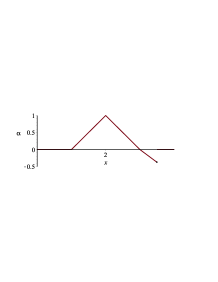
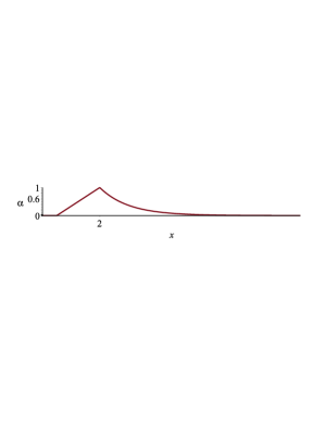
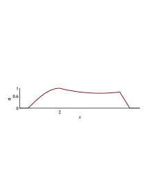
Figure 2. Functions which do not characterize fuzzy numbers: (a) function with negative values, (b) function with unbounded support, (c) monotonicity condition not fulfilled.

Remark 1.1.

In the scientific community dealing with fuzzy numbers it is customary to denote the values of characterizing functions by $\alpha$ (not e.g. $y$), where $0\leq\alpha\leq 1$. When analyzing graphs of fuzzy numbers one needs to be ever conscientious about whether and to what degree the ordinate axis is scaled. (We shall later see that $\operatorname{supp}[\xi\odot\eta]=\operatorname{supp}[\xi]\cdot\operatorname{supp}[\eta]$.) In this presentation we shall look at “small” numbers and as a rule employ non-scaled graphs.

1.1. Addition and multiplication on $\mathcal{F}_{c}^{0}(\mathbb{R}^{+})$

Remark 1.2.

Because of the monotonicity conditions (1.3), (1.4) of Definition 1 the fuzzy components $\xi_{l}$ and $\xi_{r}$ of $\xi$ are invertible with $\xi_{l}^{-1}:[0,1]\to\mathbb{R}$ with $\xi_{l}^{-1}(\mathbb{R})=[l,m]$ and $\xi_{r}^{-1}:[0,1]\to\mathbb{R}$ with $\xi_{r}^{-1}(\mathbb{R})=[m,r]$, which are again invertible and those new inverses are once more strictly monotone and have values $\alpha\in[0,1]$ and we may write:

1.1.1. Addition

of fuzzy numbers is defined in the following way:

(1.2) $$\begin{split}(\xi\oplus\eta)_{l}(x)\,=\,(\xi_{l}^{-1}+\eta_{l}^{-1})^{-1}(x),\\ (\xi\oplus\eta)_{r}(x)\,=\,(\xi_{r}^{-1}+\eta_{r}^{-1})^{-1}(x).\end{split}$$

This implies that $(\xi\oplus\eta)(m)=1$, where $m=\>\xi^{-1}(1)+\eta^{-1}(1)$, so using the notation of Definition 1’ we have

(1.3) $$\mbox{$(\xi\oplus\eta)_{m}=\xi_{m}+\eta_{m}$}.$$

In interval notation (Definition 1”) we write:

(1.4) $$(\xi_{l},\xi_{r})\oplus(\eta_{l},\eta_{r})=\biggl{(}(\xi_{l}^{-1}+\eta_{l}^{-1})^{-1}\,\textbf{,}\,(\xi_{r}^{-1}+\eta_{r}^{-1})^{-1}\biggr{)}$$

Remark 1.3.

The operation given in (1.2) is well defined since being the sum of strictly monotone functions $(\xi_{l}^{-1}+\eta_{l}^{-1})$ and $(\xi_{r}^{-1}+\eta_{r}^{-1})$ are also strictly monotone and therefore are invertible on their natural domain $[0,1]$.

1.1.2. Multiplication

is defined analogically

(1.5) $$\begin{split}(\xi\odot\eta)_{l}(x)\,=\,(\xi_{l}^{-1}\cdot\eta_{l}^{-1})^{-1}(x),\\ (\xi\odot\eta)_{r}(x)\,=\,(\xi_{r}^{-1}\cdot\eta_{r}^{-1})^{-1}(x).\end{split}$$

With

(1.6) $$(\xi\odot\eta)(m)\,=\>1\,\quad\text{where \>$m=\>\xi^{-1}(1)\cdot\eta^{-1}(1)$},$$

or

(1.7) $$(\xi\odot\eta)_{m}=\xi_{m}\cdot\eta_{m}.$$

and again

(1.8) $$(\xi_{l},\xi_{r})\odot(\eta_{l},\eta_{r})=\left((\xi_{l}^{-1}\cdot\eta_{l}^{-1})^{-1},(\xi_{r}^{-1}\cdot\eta_{r}^{-1})^{-1}\right)$$

The formulae for addition and multiplication of fuzzy numbers given above may be explicated in a convenient albeit quite informal way:

A fuzzy $5$ times a fuzzy $3$ is a fuzzy $15$ and their sum is a fuzzy $8$. The tricky part is to compute the left and right fuzzy parts: Here is what you do:

Draw the graphs of the two fuzzy numbers on a piece of paper acting as the the coordinate plane of $x$ and $\alpha$. Rotate the piece of paper by 90 degrees to interchange the roles of $x$ and $\alpha$. Add or multiply in standard manner as functions the components of the rotated functions. Rotate back the coordinate plane to see the outcome.

1.2. Algebraic properties of $\mathcal{F}_{c}^{0}(\mathbb{R}^{+})$

It follows directly from the definition that the operations of addition “$\oplus$” and multiplication “$\odot$” are commutative and associative, i.e. for arbitrary $\xi,\eta,\mu\in\mathcal{F}_{c}^{0}(\mathbb{R}^{+}),$

$$\begin{split}\xi\oplus\eta&=\eta\oplus\xi\quad\text{ and }\quad\xi\odot\eta=\eta\odot\xi.\\ (\xi\oplus\eta)\oplus\mu&=\eta\oplus(\xi\oplus\mu)\quad\text{ and }\quad(\xi\odot\eta)\odot\mu=\eta\odot(\xi\odot\mu).\end{split}$$

Moreover, the standard distributive property

(1.9) $$\xi\odot(\eta\oplus\mu)=(\xi\odot\eta)\oplus(\xi\odot\mu)$$

is satisfied as well. (for (1.9) to hold, it is essential that the support of the characterizing functions be contained in the positive reals. Distributivity will not hold for the extension of section 3).

We shall close this section with several examples illustrating the operations of addition and multiplication.

Example 1.

The simplest examples of fuzzy numbers, and those that appear in the literature most often, are numbers whose fuzzy endpoints are linear. (Such numbers are commonly referred to as “triangle numbers” and in short denoted by $tr_{(l,m,r)}(\cdot)$. So let us consider two such fuzzy numbers $\xi$ and $\eta$ defined by their characterizing functions:

(1.10) $$\xi(x)=\begin{cases}\xi_{l}(x)=x-1&\text{ for $x\in[1,2],$}\\ 1&\text{ for $x=2$},\\ \xi_{r}(x)=3-x&\text{ for $x\in[2,3],$}\end{cases}$$

and

(1.11) $$\eta(x)=\begin{cases}\eta_{l}(x)=\frac{1}{2}x-\frac{5}{2}&\text{ for $x\in[5,7],$}\\ 1&\text{ for $x=7$},\\ \eta_{r}(x)=-\frac{1}{3}x+\frac{10}{3}&\text{ for $x\in[7,10].$}\end{cases}$$

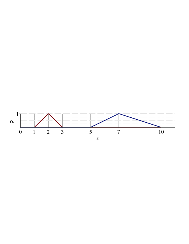
Figure 3. Two fuzzy numbers $\xi$ and $\eta$ with linear fuzzy endpoints.

Now whether we want to add or multiply $\xi$ and $\eta$ we need to first find the inverse functions $\xi_{l}^{-1},\xi_{r}^{-1}$ and $\eta_{l}^{-1},\eta_{r}^{-1}\,$:

$$\xi_{l}^{-1}(\alpha)=\,\, \alpha+1, \eta_{l}^{-1}(\alpha)=\, 2\alpha+5,$$

$$\xi_{r}^{-1}(\alpha)=\,\, 3-\alpha, \eta_{r}^{-1}(\alpha)=\, 10-3\alpha.$$

To perform the addition we use (1.2). For $\alpha\in[0,1]$ we obtain

$$\xi_{l}^{-1}(\alpha)+\eta_{l}^{-1}(\alpha)= \,3\alpha+6,$$

$$\xi_{r}^{-1}(\alpha)+\eta_{r}^{-1}(\alpha)= \,13-4\alpha.$$

Thus, inverting once again by (1.2) we arrive at

$$\xi\oplus\eta\,(x)=\begin{cases}(\xi\oplus\eta)_{l}(x)=\frac{1}{3}x-2&\text{ for $x\in[6,9],$}\\ 1&\text{ for $x=9,$}\\ (\xi\oplus\eta)_{r}(x)=-\frac{1}{4}x+\frac{13}{4}&\text{ for $x\in[9,13].$}\end{cases}$$

with $(\xi\oplus\eta)_{m}=\xi_{m}+\eta_{m}=2+7=9$.

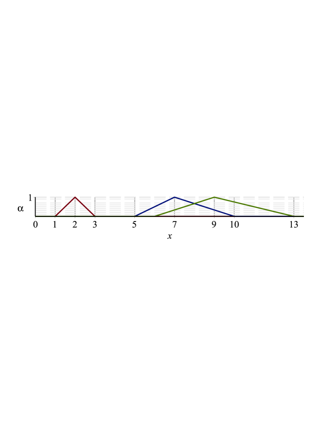
Figure 4. Two fuzzy numbers $\xi$, $\eta$ and their sum $\xi\oplus\eta$

Fig. 4 shows $\xi$, $\eta,$ and $\xi\oplus\eta.$ We note that the fuzzy addition operation “$\oplus$” preserves linearity of components.

Now let us move on to multiplication. Going by (1.5) we get

$$\xi_{l}^{-1}(\alpha)\cdot\eta_{l}^{-1}(\alpha)=\,\, 2\alpha^{2}+7\alpha+5,$$

$$\xi_{r}^{-1}(\alpha)\cdot\eta_{r}^{-1}(\alpha)=\,\, 3\alpha^{2}-19\alpha+30.$$

for $\alpha\in[0,1].$ We now need to find the inverse functions of the obtained products. For the function $\xi_{l}^{-1}(\alpha)\cdot\eta_{l}^{-1}(\alpha)$ we have $2\alpha^{2}+7\alpha+5=x.$ Since $\alpha$ changes between 0 and 1, we see that $x$ changes between $5$ and $14.$ Thus we need to solve the quadratic equation $2\alpha^{2}+7\alpha+5-x=0$ for $\alpha\in[0,1]$ and $x\in[5,14]$. We calculate the discriminant $\Delta=9+8x$ and see that $\alpha=\frac{-7+\sqrt{9+8x}}{4}$ for $x\in[5,14].$ The function $\xi_{r}^{-1}(\alpha)\cdot\eta_{r}^{-1}(\alpha)$ can be inverted in a similar way (the details are left as an exercise for the reader). Clearly, $(\xi\odot\eta)_{m}=\xi_{m}\cdot\eta_{m}=2\cdot 7=14$, so finally we obtain

$$(\xi\odot\eta)(x)=\begin{cases}(\xi\odot\eta)_{l}(x)=\frac{-7+\sqrt{9+8x}}{4}&\text{ for $x\in[5,14],$}\\ 1&\text{ for $x=14,$}\\ (\xi\odot\eta)_{r}(x)=\frac{19-\sqrt{1+12x}}{6}&\text{ for $x\in[14,30].$}\end{cases}$$

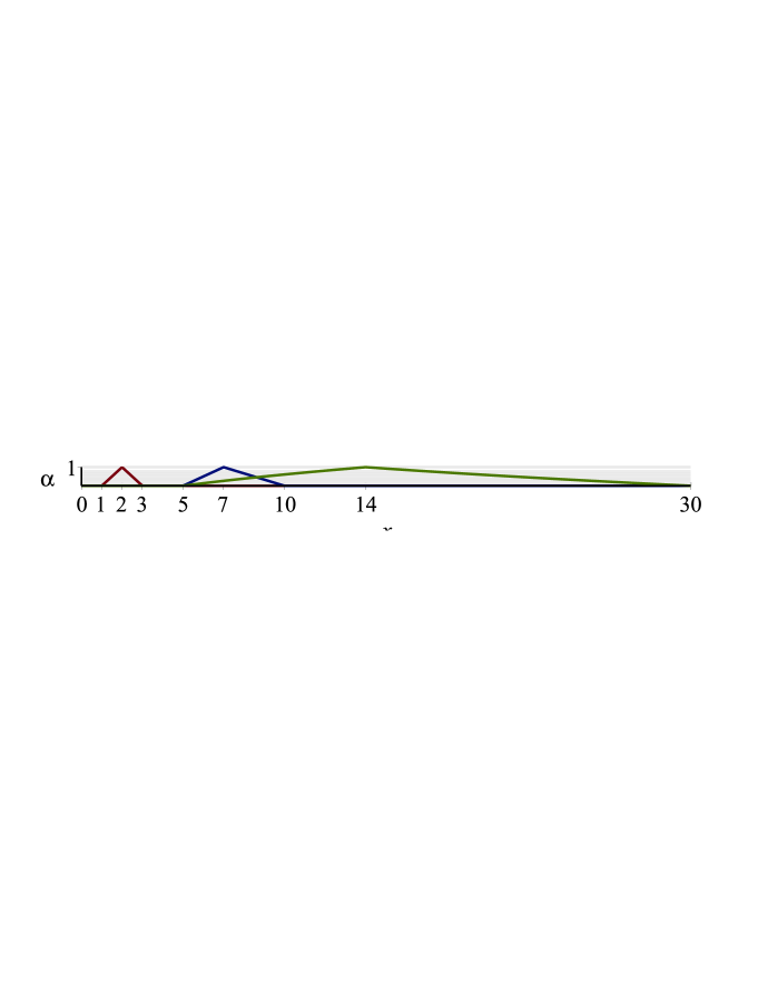
Figure 5. Fuzzy numbers $\xi$, $\eta$ and their product $\xi\odot\eta$.

Remark 1.4.

The product $\xi\odot\eta$ of two fuzzy numbers with linear characterizing functions has components that are not linear, but are rather of a square root type.

Example 2.

Let us consider the fuzzy number $\xi(x)=\chi_{[0,\pi]}(x)\cdot\sin x$ and decompose and write it in the form of Definition 1’:

$$\xi(x)=\begin{cases}\sin x&\text{ for $x\in[0,\frac{\pi}{2}],$}\\ 1&\text{ for $x=\frac{\pi}{2}$}\\ \sin x&\text{ for $x\in[\frac{\pi}{2},\pi].$}\end{cases}$$

We would like to calculate $\xi\odot\xi$, that is, $\sin^{\odot 2}$. We have $\xi_{l}(x)=\sin x$ for $x\in[0,\frac{\pi}{2}]$ and $\xi_{r}(x)=\sin x$ on $[\frac{\pi}{2},\pi].$ Thus $\xi_{l}^{-1}(\alpha)=\arcsin\alpha$ for $\alpha\in[0,1],$ and $\xi_{r}^{-1}(\alpha)=\pi-\arcsin(\alpha)$ for $\alpha\in[0,1].$ Both these functions are shown in Fig. 6.

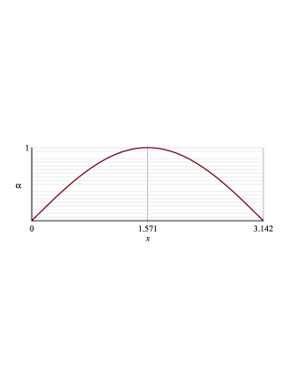
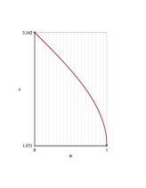
Figure 6. (a) the function $\xi(x)=\chi_{[0,\pi]}(x)\sin x,$ (b) the inverse $\xi_{l}^{-1}(\alpha),$ (c) the inverse $\xi_{r}^{-1}(\alpha).$

In order to find $(\xi\odot\xi)_{l}$ we need to invert the function $x=\arcsin^{2}\alpha$. Similarly, for $(\xi\odot\xi)_{r}$ we need to invert $x=(\pi-\arcsin(\alpha))^{2}.$ In this way we obtain

$$\xi\odot\xi\,(x)=\begin{cases}(\xi\odot\xi)_{l}(x)=\sin(\sqrt{x})&\text{ for $x\in[0,\frac{\pi^{2}}{4}],$}\\ 1&\text{ for $x=\frac{\pi^{2}}{4},$}\\ (\xi\odot\xi)_{r}(x)=\sin(\pi-\sqrt{x})=\sin(\sqrt{x})&\text{ for $x\in[\frac{\pi^{2}}{4},\pi^{2}].$}\end{cases}$$

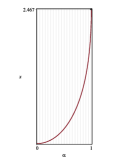
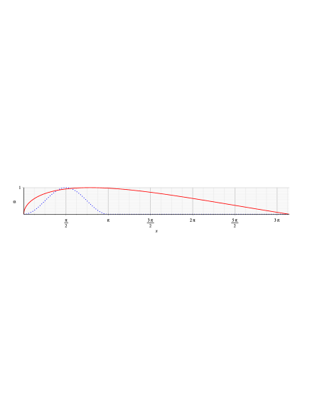
Figure 7. $(\xi^{-1}_{l})^{2},(\xi^{-1}_{r})^{2}$ and $\sin^{\odot 2}$. For comparison (dotted blue line) $\sin^{2}$.

Remark 1.5.

We see that in the realm (domain) of fuzzy numbers we have an identity $\sin^{\odot 2}(x)=\sin(\sqrt{x})$ with supports $[0,\pi]$ and $[0,\pi^{2}]$ respectively.

- This is not a coincidence but an example indicating of how functions of fuzzy quantities work.

Example 3.

Let $\xi$ be as in the previous example, that is, $\xi(x)=\chi_{[0,\pi]}(x)\sin x$ and $\eta(x)=\chi_{[\frac{3\pi}{2},\frac{5\pi}{2}]}\cos x.$ For $\eta$ we have $\eta_{l}^{-1}(\alpha)=\arcsin(\alpha)+\frac{3}{2}\pi$ and $\eta_{r}^{-1}(\alpha)=\arcsin(-\alpha)+5\pi/2$ for $\alpha\in[0,1].$ Thus, we invert the functions $x=\arcsin(\alpha)(\arcsin\alpha+3\pi/2)$ and $x=(\arcsin(-\alpha)+\pi)(\arcsin(-\alpha)+5\pi/2)$ to arrive at (see Fig. 8)

$$\xi\odot\eta=\begin{cases}(\xi\odot\eta)_{l}=\sin\left(-\frac{3}{4}\pi+\frac{1}{2}\sqrt{\frac{9}{4}\pi^{2}+4x}\right)&\text{ for $x\in[0,\pi^{2}],$}\\ 1&\text{ for $x=\pi^{2},$}\\ (\xi\odot\eta)_{r}=\sin\left(\frac{7}{4}\pi-\frac{1}{2}\sqrt{\frac{9}{4}\pi^{2}+4x}\right)&\text{ for $x\in[\pi^{2},5\pi^{2}/2].$}\end{cases}$$

or in one piece

$$\xi\odot\eta=\chi_{[0,\frac{5}{2}\pi^{2}]}(x)\cdot-\sin(\frac{1}{4}\pi+\frac{1}{4}\sqrt{9\pi^{2}+16x})$$

Figure 8. $\xi(x)=\chi_{[0,\pi]}(x)\sin x$, $\eta(x)=\chi_{[3\pi/2,5\pi/2]}\cos x,$ and the product $\xi\odot\eta$.

2. $\mathcal{F}_{c}(\mathbb{R}^{+})$

In section 1 we defined a class of fuzzy numbers $\mathcal{F}_{c}^{0}(\mathbb{R}^{+})$, where the subscript “$c$” stands for “compact” to indicate that the characterizing functions defining the fuzzy numbers have compact support, and the superscript “$0$” indicates that these functions are also continuous.

Notably the real numbers $\mathbb{R}$ are beyond the scope of Definition 1. In this section a second, wider definition is brought in to include the standard real numbers and also the interval numbers (that is, the characteristic functions of intervals). Thus, we will allow a characterizing function $\xi(\cdot)$ to be equal to $1$ on a closed interval $[\underline{m},\overline{m}]$ (in the class $\mathcal{F}_{c}^{0}(\mathbb{R}^{+})$ we had $\underline{m}=\overline{m}$). Our findings and statements will henceforth be formulated for “fuzzy intervals” and we will refer to fuzzy numbers as to the subcase when $\underline{m}=\overline{m}=m$.

Moreover, we shall no longer require that the fuzzy endpoints $\xi_{l}$ and $\xi_{r}$ be strictly monotone and continuous, and instead require only simple monotonicity and semi-continuity.

This new class shall be denoted by $\mathcal{F}_{c}(\mathbb{R}^{+}).$

Definition 2.

A fuzzy interval $\xi$ from the class $\mathcal{F}_{c}(\mathbb{R}^{+})$ is characterized by a function $\xi(\cdot):\mathbb{R}^{+}\to[0,1]$ with the following properties:

• compact support: the closure of the points $x\in\mathbb{R}^{+}$, where $\xi(x)>0$ is a closed interval $[l,r]\subset\mathbb{R}^{+},$

• The set of points $x\in\mathbb{R}^{+}$ where the characterizing function $\xi(\cdot)$ attains value $1$ is a closed interval $[\underline{m},\overline{m}]\subset[l,r]$, in other words

  $\{x\in\mathbb{R}:\xi(x)=1\}=[\underline{m},\overline{m}]\subseteq[l,r]$

• the function $\xi_{l}(x):=\xi(x)$ for $x\in[l,\underline{m}]$ is non-decreasing and right-continuous,

• the function $\xi_{r}(x):=\xi(x)$ for $x\in[\overline{m},r]$ is non-increasing and left-continuous.

Remark 2.1.

Note that conditions $(1)-(4)$ in Definition 2 imply that $\xi(\cdot)$ is upper semi-continuous, that is

$$\limsup_{x\to x_{0}}\xi(x)\leq\xi(x_{0}),\quad\forall x_{0}\in\mathbb{R}^{+}.$$

As in section 1 and Definition 1’ (1.1) the characterizing function of a fuzzy interval $\xi\in\mathcal{F}_{c}(\mathbb{R}^{+})$ can be rewritten as

Definition 2’.

(2.1) $$\xi(x)=\begin{cases}\xi_{l}(x)&\text{ for $x\in[l,\underline{m}],$}\\ 1&\text{ for $x\in[\underline{m},\overline{m}],$}\\ \xi_{r}(x)&\text{ for $x\in[\overline{m},r].$}\end{cases}$$

(Again $\xi_{l}(\underline{m})=\xi_{r}(\overline{m})=1$ is an overkill, but we need this for inversion)

As in the preceding section a fuzzy interval (number) is uniquely determined by its fuzzy components $\xi_{l}$ and $\xi_{r}$. The interval $[\underline{m},\overline{m}]$ need not be stated explicitly, but usually will be for sake of clarity.

Definition 2” Again a representation by an ordered pair $\left(\xi_{l},\xi_{r}\right)$ where $\xi_{l}$ and $\xi_{r}$ meet the conditions of Definition 2 above seems intuitive and highly desirable, especially when speaking of fuzzy intervals (not fuzzy numbers).

As we mentioned before, the class $\mathcal{F}_{c}(\mathbb{R}^{+})$ includes the standard positive numbers $\mathbb{R}^{+}$ and the interval numbers. Indeed, every $\lambda\in\mathbb{R}^{+}$ can be identified with the delta function $\delta_{\lambda}:\mathbb{R}^{+}\to\{0,1\}$ such that $\delta_{\lambda}(x)=1$ iff $x=\lambda$ and $0$ elsewhere. (Convention: We use $\chi_{\{\lambda\}}$ and $\delta_{\lambda}(x)$ interchangeably). Clearly, $\delta_{\lambda}\in\mathcal{F}_{c}(\mathbb{R}^{+})$, which can be seen by taking $l=\underline{m}=\overline{m}=r=\lambda$ and $\xi_{l}=\xi_{r}=\chi_{\{\lambda\}}$ in Definition 2’. For an interval number interpreted as its own characteristic function $\chi_{[a,b]}$ of the interval $[a,b]\subset\mathbb{R}^{+}$ the understanding is the same. We have $\chi_{[a,b]}\in\mathcal{F}_{c}(\mathbb{R}^{+})$, which can be seen by taking $l=\underline{m}=a$ and $b=\overline{m}=r$ and $\xi_{l}=\chi_{\{a\}},\xi_{r}=\chi_{\{b\}}$ in Definition 2’.

We shall see later that the arithmetic which will be defined below for $\mathcal{F}_{c}(\mathbb{R}^{+})$ is consistent with the standard arithmetic of $\mathbb{R}^{+}$, as well as the set arithmetic for intervals.

2.1. Generalized Inverse Function

The (not strictly) monotone and/or possibly discontinuous functions $\xi_{l}$, $\xi_{r}$ of Definition 2’ may not be invertible in the classical sense. In order to be able to employ, as before in section 1 formulae analogous to (1.2) and (1.5) in defining the operations “$\oplus$”,“$\odot$” we shall presently introduce and then apply the notion (appearing in statistics in the form of generalized inverses of CDFs, or quantile functions) of a generalized inverse function:

Take a function $h:I\mapsto[0,1]$ defined on a closed interval $I$, that is one-sided continuous and non-strictly monotone.parThe price to pay for relaxing the conditions of continuity and strict monotonicity and instead assuming only one-sided continuity and non-strict monotonicity is that we encounter two types of problems in the process of finding a useful inverse function in the classical sense:

1. There is a point $x_{0}$, where the function $h$ has a jump discontinuity.

   Such a function function is invertible in the classical sense, but the domain of its inverse function will not be the full interval $[0,1]$.

   Now two functions ${h_{1}},{h_{2}}$ with jump discontinuities at different points will produce inverse functions ${h_{1}}^{-1},{h_{2}}^{-1}$ of different domains $h_{1}(I)$ and $h_{2}(I).$ - Therefore, (1.2), and (1.5) cannot be applied because the addition or multiplication of functions with different domains is simply not well defined.

2. The function $h$ is constant on some interval $[\underline{x}_{0},\overline{x}_{0}]$.

   In this case the function is not injective, and therefore not invertible at all in the classical sense.

In order to overcome these problems and to be able to extend formulae (1.2) and (1.5) we shall, for our present purposes, single out two types of generalized inverse functions. For a non-decreasing right-continuous function $f:I\to J$ defined on on a closed interval $I$ and taking values in a closed interval $J$ (resp. non-increasing left-continuous function $g:I\to J$) we define two types of generalized inverse functions by

(2.2) $$f_{\inf}^{-1}(\alpha)=\begin{cases}\vspace{1mm}\inf\{x:\xi_{l}(x)\geq\alpha\}\quad\text{for}\,\alpha\in(0,1],\\ \underline{\operatorname{supp}(\xi_{l})}\quad\text{for}\,\alpha=0,\end{cases}$$

and

(2.3) $$f_{\sup}^{-1}(\alpha)=\begin{cases}\vspace{1mm}\sup\{x:\xi_{r}(x)\geq\alpha\}\quad\text{for}\,\alpha\in(0,1],\\ \overline{\operatorname{supp}(\xi_{r})}\quad\text{for}\,\alpha=0.\end{cases}$$

To see how concretely the generalized inverse procedure works in practice let us consider the case of a non-decreasing right-continuous function $f$ (which may serve as the left fuzzy endpoint $\xi_{l}$ of a fuzzy interval $\xi$ as in Definition 2).

1. Let $f$ be a non-decreasing right-continuous function with a jump discontinuity at the point $x_{0}$. Let $f(x_{0})=\alpha_{0}$. Let us set $\overline{\alpha}_{0}=\alpha_{0}$ and $\underline{\alpha}_{0}=\sup\{f(x):x<x_{0}\}$. Then for all $\alpha\in(\underline{\alpha}_{0},\overline{\alpha}_{0}]$ we have that

   $$f_{\inf}^{-1}(\alpha)=\inf\{x:f(x)\geq\alpha\}=x_{0},$$

   that is, the generalized inverse function is constant on the half-closed interval $(\underline{\alpha}_{0},\overline{\alpha}_{0}]$.

2. Let $f$ be constant on the interval $[\underline{x}_{0},\overline{x}_{0})$ with $f(x)=\alpha_{0}$ for $x$ in the interval. In this case clearly,

   $$f_{\inf}^{-1}(\alpha_{0})=\inf\{x:f(x)\geq\alpha_{0}\}=\underline{x}_{0},$$

   while

   $$\inf\{f_{\inf}^{-1}(\alpha):\alpha>\alpha_{0}\}=\overline{x}_{0}.$$

   Thus, the generalized inverse has a jump discontinuity at $\alpha_{0}$.

For a (not strictly) decreasing function $g$, which in what is coming may serve as the right fuzzy component of a fuzzy interval $\xi$ the reasoning is analogous, except that “$\inf$” on each occurrence must be replaced by “$\sup$”, and right-closed intervals be substituted by left-closed ones and vice-versa.

In the light of the above we see that the procedure of finding the generalized inverse works may be unceremoniously summarized: Jump discontinuities of the input convert to intervals where the output inverted function is constant. And the intervals where the input is constant convert to jump discontinuities of the output. These two observations are illustrated below for fragments of two possible left fuzzy endpoints (green) and their inverses (blue) :

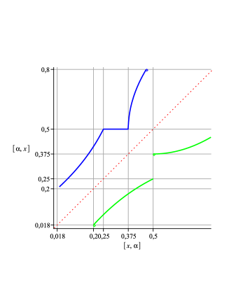
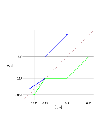
Figure 9. jump-discontinuity converts to constant, constant to jump-discontinuity

Again for a non-increasing left-continuous function $g$ serving as the right fuzzy part $\xi_{r}$ of a fuzzy interval $\xi$ given as in Definition 2 the procedure of finding the general inverse works analogously substituting “$\sup$” for “$\inf$”.

Remark 2.2.

We also explicitly note, that for a left fuzzy component $\xi_{l}(\cdot)$ which is by definition increasing and right-continuous its generalized inverse

${\xi_{l}}^{-1}_{\inf}:[0,1]\to\mathbb{R}^{+}$ is still increasing (only fuzzy convexity i.e.: $\xi(\lambda x_{1}+(1-\lambda)x_{2})\geq\min\bigl{(}\xi(x_{1}),\xi(x_{2})\bigr{)}$ transforms into concavity), but left-continuous.

Observe also that ${\xi_{l}}^{-1}_{\inf}(0)=l$, ${\xi_{l}}^{-1}_{\inf}(1)=\underline{m}$.

Likewise ${\xi_{r}}^{-1}_{\sup}:[0,1]\to\mathbb{R}^{+}$ is a decreasing, right-continuous function and

${\xi_{r}}^{-1}_{\sup}(1)=\overline{m}$ and ${\xi_{r}}^{-1}_{\sup}(r)=0.$

2.1.1. Graphs illustrating generalized inversion

In what follows some example graphs are displayed:

The infimum and supremum inverse of a real number $\lambda$ understood as the fuzzy number $\chi_{\{\lambda\}}$ or equivalently the delta function $\delta_{\lambda}$ is the constant function $\alpha=\lambda$ (with domain $[0,1]$):

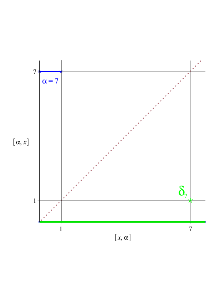
Figure 10. inverse (infimum and supremum) of a real number

Below the infimum and supremum generalized inverses (blue) of a stepfunction (green) are confronted for comparison:

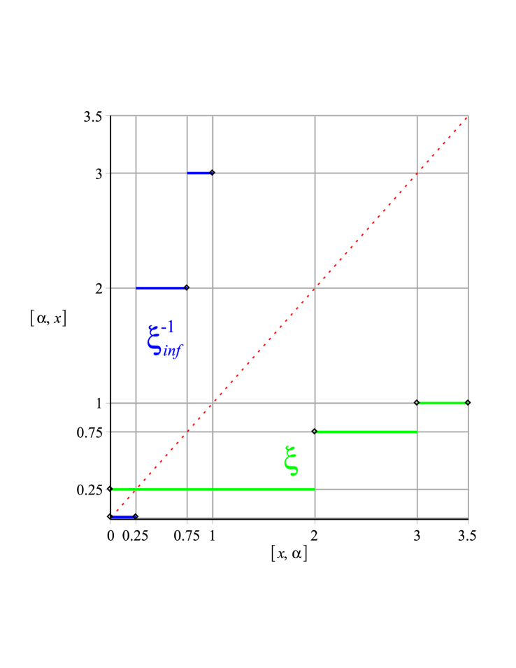
(a) infimum inverse of a step function (green)

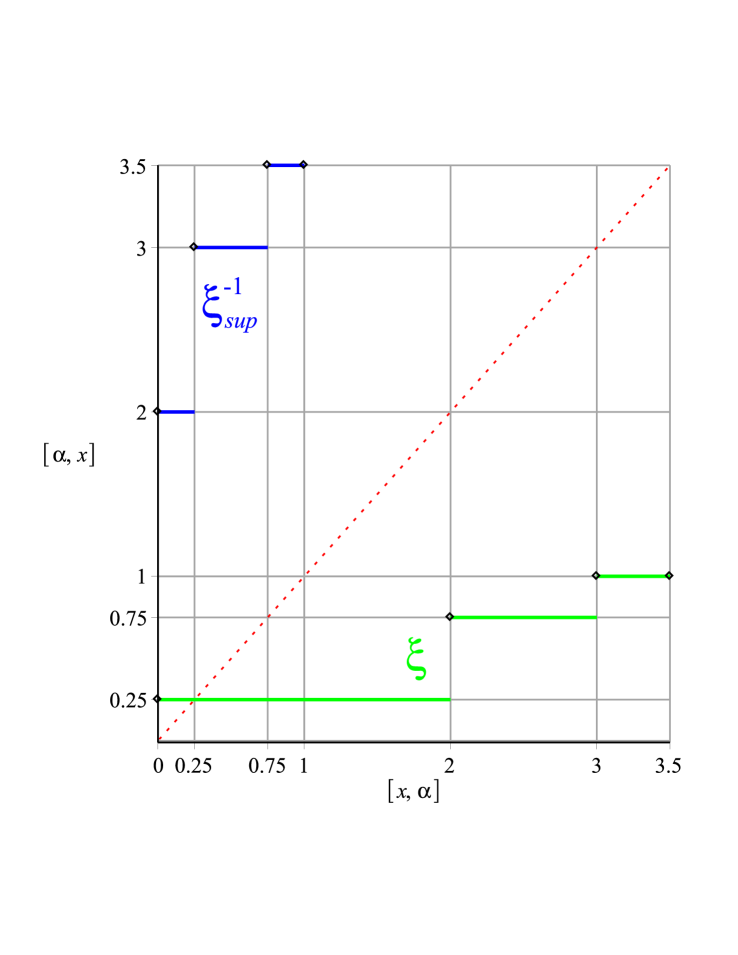
(b) supremum inverse of the same step function

As a final example illustrating the procedure of generalized inversion here is now a freely patched together “fantasy” function which includes both jumps and constant parts and its generalized inverse:

$${fanta}_{l}(x)=\begin{cases}\frac{1}{4}x\quad&x\in[\frac{1}{4},\frac{2}{3})\\ \sin(3x-\frac{1}{2})\quad&x\in[\frac{2}{3},\frac{6}{7})\\ \frac{5}{8}\quad&x\in[\frac{6}{7},\frac{9}{8})\\ \frac{5}{6}x\quad&x\in[\frac{9}{8},\frac{6}{5}]\end{cases}$$

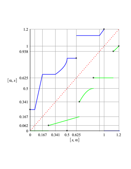
Figure 12. the infimum generalized inverse (blue) of a “fantasy” function (green)

$${fanta}_{d}(\alpha)=\begin{cases}\frac{1}{4}\quad&\alpha\in[0,\frac{1}{16}]\\ 4\alpha\quad&\alpha\in(\frac{1}{16},\frac{1}{6}]\\ \frac{2}{3}\quad&\alpha\in(\frac{1}{6},\sin(1)-\frac{1}{2}]\\ \tiny\frac{1}{3}\arcsin(\alpha+\frac{1}{2})+\frac{1}{3}&\alpha\in(\sin(1)-\frac{1}{2},\sin(\frac{11}{7})-\frac{1}{2}]\\ \frac{1}{6}\quad&\alpha\in(\sin(\frac{11}{7})-\frac{1}{2},\frac{5}{8}]\\ \frac{9}{8}\quad&\alpha\in(\frac{5}{8},\frac{15}{16}]\\ \frac{6}{5}\alpha\quad&\alpha\in(\frac{15}{16},1]\end{cases}$$

2.2. Re-inversion of fuzzy endpoints

To reduce the multitude of sub- and superscripts and indices let us first introduce some shorthand notation:

Notation.

1. Set ${\xi_{l}}^{-1}_{\inf}=:\xi_{d}$ as in downwards fuzzy, and

2. set ${\xi_{l}}^{-1}_{\inf}=:\xi_{d}$ as in upwards fuzzy

To be able to adapt formulae 1.2 and 1.5 to the present case we need to define an suitable re-inversion-operator for the generalized inversion function. One basic prerequisite condition which must be expected from this operator, which we will denote by and overhead left arrow $``\overleftarrow{(\cdot)}"$ is that

$$\overleftarrow{(\xi_{d})}(x)=\xi_{l}(x)\text{\quad and \quad}\overleftarrow{(\xi_{u})}(x)=\xi_{r}(x).$$

2.2.1. Inversion and re-inversion of a fuzzy left endpoint $\xi_{l}(\cdot)$

For easy reference recall that for $\xi_{l}:\mathbb{R}\mapsto[0,1]$ onto, non-decreasing and left-continuous its generalized inverse function is defined by:

(2.4) $$\xi_{d}(\alpha)=\begin{cases}\vspace{1mm}\inf\{x:\xi_{l}(x)\geq\alpha\}\quad\text{for}\>\alpha\in(0,1],\\ \underline{\operatorname{supp}(\xi_{l})}\quad\text{for}\>\alpha=0.\end{cases}$$

Remark 2.3.

Note, that for $\xi_{l}$ onto, strictly monotonic (increasing) and continuous the definitions of generalized and classical inversion coincide:

(2.5) $$\xi_{d}=\xi_{l}^{-1}.$$

Remark 2.4.

Remember, that the generalized inverse $\xi_{d}$ of the non-decreasing, left-continuous function $\xi_{l}$ is again a non-decreasing function, but right-continuous.

Now define a re-inversion operator for the generalized inverse of a left fuzzy endpoint by:

(2.6) $$\overleftarrow{\xi_{d}}(x)=\begin{cases}\vspace{1mm}\inf\{\alpha:\xi_{d}(\alpha)>x\}\quad\text{for}\,x\in\left[\underline{\operatorname{supp}(\xi_{l})},\overline{\operatorname{supp}(\xi_{l})}\right),\\ \vspace{1mm}1\quad\text{for}\,x=\overline{\operatorname{supp}(\xi_{l})},\\ 0\quad\text{for}\,x\notin\operatorname{supp}(\xi_{l}).\end{cases}$$

It is then easy to see that

Lemma 2.5.

(2.7) $$\overleftarrow{(\xi_{d})}(x)=\xi_{l}(x).$$

Proof.

The proof follows the reasoning applied in the preceding section 2.1 ∎

Remark 2.6.

Note that for the strictly monotonic and continuous case (2.7) reads just

(2.8) $$(\xi_{l}^{-1})^{-1}=\xi_{l}.$$

We now proceed analogously with the right fuzzy endpoint:

2.2.2. Inversion and re-inversion of a right fuzzy endpoint $\xi_{r}(\cdot)$

We recall that the generalized inverse to the non-increasing, left-continuous right fuzzy endpoint $\xi_{r}:\mathbb{R}\mapsto[0,1]$ is given by:

(2.9) $$\xi_{u}(\alpha)=\begin{cases}\vspace{1mm}\sup\{x:\xi_{r}(x)\geq\alpha\}\quad\text{for}\,\alpha\in(0,1],\\ \overline{\operatorname{supp}(\xi_{r})}\quad\text{for}\,\alpha=0.\end{cases}$$

Remark 2.7.

Obviously for $\xi_{r}$ strictly decreasing and continuous the equality

(2.10) $$\xi_{u}=\xi_{r}^{-1}$$

will hold.

Remark 2.8.

Note, that the generalized inverse $\xi_{u}$ of the non-increasing, right-continuous function $\xi_{l}$ is again a non-increasing function, but left-continuous.

And we define re-inversion by setting:

(2.11) $$\overleftarrow{(\xi_{u})}(x)=\begin{cases}\vspace{1mm}\sup\{\alpha:\xi_{u}(\alpha)>x\}\quad\text{for}\,x\in\operatorname{supp}(\xi_{r}),\\ 0\quad\text{for}\,x\notin\operatorname{supp}(\xi_{r}).\end{cases}$$

Lemma 2.9.

Then: $\overleftarrow{(\xi_{u})}(x)=\xi_{r}(x).$

Proof.

As above. ∎

With this the requisite apparatus for extending the definitions of section 1 has been established and we may proceed:

2.3. Addition and multiplication in $\mathcal{F}_{c}(\mathbb{R}^{+})$

Addition and multiplication in $\mathcal{F}_{c}(\mathbb{R}^{+})$ are defined in the same way as in the class $\mathcal{F}_{c}^{0}(\mathbb{R}^{+})$, namely we extend formulae (1.2) and (1.5) by application of the generalized inverse functions as defined in (2.4) and (2.9):

We set

(2.12) $$\begin{split}(\xi\oplus\eta)_{l}=\overleftarrow{(\xi_{d}+\eta_{d})}\\ (\xi\oplus\eta)_{r}=\overleftarrow{(\xi_{u}+\eta_{u})}\end{split}$$

and

(2.13) $$\begin{split}(\xi\odot\eta)_{l}=\overleftarrow{(\xi_{d}\cdot\eta_{d})}\\ (\xi\odot\eta)_{r}=\overleftarrow{(\xi_{u}\cdot\eta_{u})}\end{split}$$

Notation.

To keep the text homogeneous in the further the above notation, i.e. subscripts “d,u”, for generalized inversion of discontinuous and/or not strictly monotonous fuzzy endpoints, and the overhead arrow symbol “$\overleftarrow{}$” for generalized re-inversion will be applied also to endpoints which are actually invertible in the classical sense.

Remark 2.10.

Clearly, the sum and the product of left-continuous (resp. right-continuous) functions are left-continuous (resp. right-continuous), thus the above operations are well defined.

Example 4 (Multiplication of interval numbers).

The basic example of a fuzzy interval is the abstraction of a real interval $A=[\underline{a},\overline{a}]$ by its characterising function $\xi_{A}=\chi_{[\underline{a},\overline{a}]}$.

Let us fuzzy multiply two interval numbers $\xi_{A}=\chi_{[2,3]}$ and $\xi_{B}=\chi_{[5,6]}.$ The result will be, as expected, $\xi_{A}\odot\xi_{B}=\chi_{[10,18]}$, as shown in Fig. 13.

Going by the definiton, one piece at a time, step by step:

(2.14) $$\begin{split}{\xi_{A}}_{\,l}=\chi_{\{2\}}\text{ for }x\in\mathbb{R}\\ {\xi_{B}}_{\,l}=\chi_{\{5\}}\text{ for }x\in\mathbb{R}\\ {\xi_{A}}_{\,d}(\alpha)=2\text{ for }\alpha\in[0,1]\\ {\xi_{B}}_{\,d}(\alpha)=5\text{ for }\alpha\in[0,1]\\ {\xi_{A}}_{\,d}(\alpha)\cdot{\xi_{B}}_{\,d}(\alpha)=2\cdot 5=10\text{ for }\alpha\in[0,1]\\ (\xi_{A}\odot\xi_{B})_{l}=\overleftarrow{{\xi_{A}}_{\,d}(\alpha)\cdot{\xi_{B}}_{\,d}(\alpha)}=\overleftarrow{(\alpha=10)}=\chi_{\{10\}}\text{ for }x\in\mathbb{R}\end{split}$$

The computation of the righthand side $(\xi_{A}\odot\xi_{B})_{r}$ is analogous.

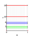
Figure 13. Multiplication of interval numbers: (a) $\xi_{A}=\chi_{[2,3]}$ and $\xi_{B}=\chi_{[5,6]},$ (b) the inverted intervals and their product, (c) the result $\xi_{A}\odot\xi_{B}=\chi_{A\cdot B}=\chi_{[10,18]}$.

In general, for $0\leq\underline{a}\leq\overline{a}$ and $0\leq\underline{b}\leq\overline{b}$ we may always use

(2.15) $$\begin{split}\chi_{[\underline{a},\overline{a}]}\odot\chi_{[\underline{b},\overline{b}]}=&\chi_{[\underline{a}\underline{b},\overline{a}\overline{b}]},\\ \chi_{[\underline{a},\overline{a}]}\oplus\chi_{[\underline{b},\overline{b}]}=&\chi_{[\underline{a}+\underline{b},\overline{a}+\overline{b}]}.\end{split}$$

which is of course perfectly consistent with classical interval arithmetic on the nonnegative reals.

Before proceeding to multiplication by a real number let us introduce some simplifying shorthand:

Notation: We write ${\delta_{\lambda}}^{-1}_{\inf}={\delta_{\lambda}}_{d}={\delta_{\lambda}}^{-1}_{\sup}={\delta_{\lambda}}_{u}=\lambda\text{ for }\alpha\in[0,1]$ or simply $\alpha=\lambda$

Example 5 (Multiplication of a fuzzy interval by a real number).

We calculate for $x\in\bigl{[}\underline{\operatorname{supp}{(\lambda\odot\xi)_{l}}},\overline{\operatorname{supp}{(\lambda\odot\xi)_{l}}}\bigr{)}$

$$\begin{split}(\lambda\odot\xi)_{l}(x)=&\;\overleftarrow{({\delta_{\lambda}}_{\,d}\cdot{\xi_{d}})}(x)=\overleftarrow{(\lambda\cdot{\xi_{d}}})(x)\\ =&\quad\inf\{\alpha:(\lambda\cdot\xi_{d})(\alpha)>x\}\\ =&\quad\inf\{\alpha:\xi_{d}(\alpha)>x/\lambda\}\\ =&\quad\overleftarrow{\xi_{d}}(x/\lambda)\\ =&\quad\xi_{l}(x/\lambda).\end{split}$$

The case $x=\overline{\operatorname{supp}{(\lambda\odot\xi)_{l}}}$ is trivial. Repeating the calculation for $\xi_{r}$, we have established the following property:

(2.16) $$(\lambda\odot\xi)(x)=\xi(x/\lambda).$$

Below

$$2\odot\chi_{[3,4]}(x)\sqrt{4-x}=\chi_{[6,8]}(x)\sqrt{4-x/2}$$

is shown as an example:

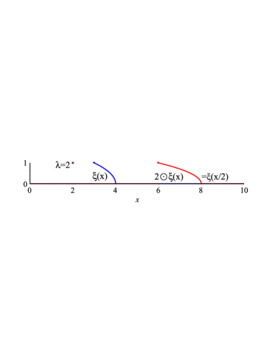
Figure 14. Multiplication of a fuzzy interval by a real number

Property (2.16) provides for the following formula which is abecedarian for statistical analysis of fuzzy data:

(2.17) $$\frac{1}{n}\odot(\xi\oplus\xi\oplus\dots\oplus\xi)=\frac{1}{n}\odot\bigoplus_{i=1}^{n}\xi=\xi,$$

Indeed,

$$\frac{1}{n}\odot\bigoplus_{i=1}^{n}\xi_{r}(x)=\frac{1}{n}\odot\overleftarrow{\left(n\odot\xi_{u}(x)\right)}=\frac{1}{n}\odot{\xi_{r}}(x/n)=\xi_{r}(x),$$

and a similar check can be done for $\xi_{l}(x)\,.$

Example 6 (Adding a real number to a fuzzy interval).

We have seen above that multiplying a fuzzy interval by a real number yields an inverse dilation of the fuzzy interval. Similarly, it can be easily shown that adding a real number to a fuzzy interval corresponds to a negative translation:

(2.18) $$(\lambda\oplus\xi)(x)=\xi(x-\lambda)\>.$$

Example 7.

In the last example of this subsection we shall provide calculations and graphs of addition and multiplication of a fuzzy interval $\xi$ and a fuzzy number $\eta$.

For $\eta$ we take the already considered function $\chi_{[0,\pi]}\cdot\sin$:

(2.19) $$\eta=\begin{cases}\eta_{l}=\sin(x)\quad&x\in[0,\frac{\pi}{2}]\\ 1&x=\frac{\pi}{2}\\ \eta_{r}=\sin(x)\quad&x\in[\frac{\pi}{2},\pi]\>.\end{cases}$$

This example’s $\xi$ has a linear part $\xi_{l}$ and a step function as $\xi_{r}$ :

(2.20) $$\xi=\begin{cases}\xi_{l}=8x-1\quad&x\in[\frac{1}{8},\frac{1}{4}]\\ \vspace{1mm}1\quad&x\in[\frac{1}{4},1]\\ \xi_{r}=\tiny\begin{cases}1&x=1\\ 0.3&x\in(1,2]\\ 0.1&x\in(2,4]\,.\end{cases}\end{cases}$$

Here the function $\xi_{r}$ is not invertible in the classical sense.

Both characterizing functions are pictured below in one graph. The middle parts are marked in dotted grey and the left and right fuzzy components are respectively green and blue.

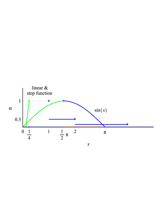
Figure 15. sine, linear and step function

We have

$${\xi_{d}}(\alpha)=\frac{1-\alpha}{8}\qquad\text{ \text{for} $\alpha\in[0,1]$ }$$

and

$${\xi_{u}}(\alpha)=\begin{cases}4\quad\text{ \text{for} }\alpha\in[0,0.1)\\ 2\quad\text{ \text{for} }\alpha\in[0.1,0.3)\\ 1\quad\text{ \text{for} }\alpha\in[0.3,1]\,.\end{cases}$$

Let us write out $\eta^{-1}(\alpha)$ as in Example 2:

$$\begin{split}{\eta_{d}}(\alpha)=&\arcsin(\alpha)\quad\text{ for $\alpha\in[0,1],$}\\ {\eta_{u}}(\alpha)=&\pi-\arcsin(\alpha)\quad\text{ for $\alpha\in[0,1]$.}\end{split}$$

We receive

$$\xi_{d}+\eta_{d}=\frac{1-\alpha}{8}+\arcsin(\alpha)\qquad\text{ for $\alpha\in[0,1]$ }$$

and

$$\xi_{u}+\eta_{u}=\begin{cases}4+\pi-\arcsin(\alpha)\quad\text{ \text{for} }x\in[0,0.1)\\ 2+\pi-\arcsin(\alpha)\quad\text{ \text{for} }x\in[0.1,0.3)\\ 1+\pi-\arcsin(\alpha)\quad\text{ \text{for} }x\in[0.3,1].\end{cases}$$

Multiplication:

$$\xi_{d}\cdot\eta_{d}=\frac{1-x}{8}\cdot\arcsin(\alpha)\qquad\text{ for $\alpha\in[0,1]$}$$

and

$$\xi_{u}\cdot\eta_{u}=\begin{cases}4\cdot(\pi-\arcsin(\alpha))\quad\text{ for }\alpha\in[0,0.1)\\ 2\cdot(\pi-\arcsin(\alpha))\quad\text{ for }\alpha\in[0.1,0.3)\\ 1\cdot(\pi-\arcsin(\alpha))\quad\text{ for }\alpha\in[0.3,1]\,.\end{cases}$$

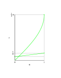
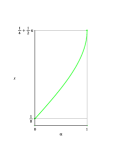
Figure 16. From left to right: $\xi_{d}(\alpha)$, $\eta_{d}(\alpha)$, $\xi_{d}(\alpha)$ and $\eta_{d}(\alpha)$, $(\xi_{d}+\eta_{d})(\alpha)$, $(\xi_{d}\cdot\eta_{d})(\alpha)$.

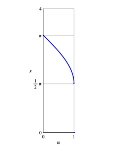
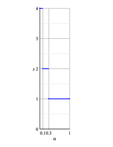
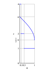
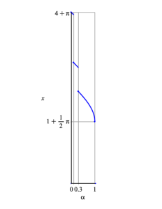
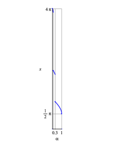
Figure 17. From left to right: $\xi_{u}(\alpha)$, $\eta_{u}(\alpha)$, $\xi_{u}(\alpha)$ and $\eta_{u}(\alpha)$, $(\xi_{u}+\eta_{u})(\alpha)$, $(\xi_{u}\cdot\eta_{u})(\alpha)$

After inverting back once more we obtain

$$\xi\odot\eta=\begin{cases}(\xi\odot\eta)_{l}=&\{\arcsin(\alpha)\cdot(\frac{\alpha-1}{8})=x\},\quad x\in[0,\frac{\pi}{8}],\,\alpha\in[0,1]\\ (\xi\odot\eta)_{m}=&[\frac{\pi}{8},\frac{\pi}{2}]\\ (\xi\odot\eta)_{r}=&\phi(x)\,,\end{cases}$$

where

$$\phi(x)=\begin{cases}\sin(1^{-1}x)\quad&x\in[(\pi-\arcsin(1))\cdot 1,(\pi-\arcsin(0.3))\cdot 1]\\ 0.3&x\in((\pi-\arcsin(0.3)\cdot 1,(\pi-\arcsin(0.3))\cdot 2]\\ \sin(2^{-1}x)&x\in((\pi-\arcsin(0.3))\cdot 2,(\pi-\arcsin(0.1))\cdot 2]\\ 0.1&x\in((\pi-\arcsin(0.1))\cdot 2,(\pi-\arcsin(0.1))\cdot 4]\\ \sin(4^{-1}x)&x\in((\pi-\arcsin(0.1))\cdot 4,(\pi-\arcsin(0))\cdot 4]\,.\end{cases}$$

Similarly

$$\xi\oplus\eta=\begin{cases}(\xi\oplus\eta)_{l}=&\{\arcsin(\alpha)+(\frac{\alpha+1}{8})=x\},\quad x\in[0,\frac{\pi}{2}+\frac{1}{8}],\alpha\in[0,1]\\ (\xi\oplus\eta)_{m}=&[\frac{\pi}{2}+\frac{1}{8},\frac{\pi}{2}+1]\\ (\xi\oplus\eta)_{r}=&\phi(x)\,,\end{cases}$$

with

$$\phi(x)=\begin{cases}\sin(x-1)\quad&x\in[(\arcsin(1)+1,(\pi-\arcsin(0.3))+1]\\ 0.3&x\in((\pi-\arcsin(0.3)+1,(\pi-\arcsin(0.3))+2]\\ \sin(x-2)&x\in((\pi-\arcsin(0.3))+2,(\pi-\arcsin(0.1))+2]\\ 0.1&x\in((\pi-\arcsin(0.1))+2,(\pi-\arcsin(0.1))+4]\\ \sin(x-4)&x\in((\pi-\arcsin(0.1))+4,(\pi-\arcsin(0))+4]\,.\end{cases}$$

Concluding the calculations of the particular components of the outcome let us notice that:

• The components $(\xi\odot\eta)_{l}$ and $(\xi\oplus\eta)_{l}$ are in a form often encountered in practice, where the function is given in implicit terms because providing a straightforward closed form representation is impossible.

• The functions $(\xi\odot\eta)_{r}$ and $(\xi\oplus\eta)_{r}$ are given in explicit terms where one could have applied (1.2) directly or simpler (2.16) and (2.18) as always taking extreme care to ascertain the proper (open or closed) endpoints of intervals.

• The middle part can be always easily written out using (2.15).

Here are the graphs of $\xi$ and $\eta$ again:

Before conducting the arithmetic operations

after addition

and after multiplication

.

2.4. Algebraic properties of the class $\mathcal{F}_{c}(\mathbb{R}^{+})$

From the general properties of functions and their inverses we see that the operations “$\oplus$” and “$\odot$” defined on $\mathcal{F}_{c}(\mathbb{R}^{+})$ are commutative and associative. We also have the zero element $\delta_{0}$ and the multiplicative identity $\delta_{1}$, so $\mathcal{F}_{c}(\mathbb{R}^{+})\cup\{\delta_{0}\}$ is a commutative semiring.

In general, the elements of $\mathcal{F}_{c}(\mathbb{R}^{+})$ do not have inverse elements, which can be easily seen in the case of interval numbers:

Indeed, for addition, using (2.15) we would have to have

$$[a,b]\oplus[x,y]=[0,0],$$

so $x=-a,y=-b$. But $[-a,-b]$ with $a<b$ does not have the right orientation meaning that the called for interval $[x,y]$ does not exist (even when allowing for negatives, as we will in section 3).

For multiplication, using (2.15) we would have to have

$$[a,b]\odot[x,y]=[1,1],$$

but $x=\frac{1}{a}\geq y=\frac{1}{b}$, meaning again there is no inverse in the strict, non-fuzzy sense. Note however that $[\frac{a}{b},\frac{b}{a}]$ will pass for a fuzzy $1$.

3. $\mathcal{F}_{c}(\mathbb{R})$

Throughout sections $1$ and $2$ we have been assuming the support of the characterizing functions to be a finite closed interval lying within $\mathbb{R}^{+}$. This assumption greatly facilitates the understanding of the essence of how fuzzy arithmetic works. In Definition 3 below this assumption is dropped. Negative and mixed (i.e. containing zero) supports are also considered. Definition 3 is what one would normally encounter in a textbook and this particular version is taken from [4]. Subsequently the definition is translated into the language used in the preceding sections.

Here is the compact form:

Definition 3.

A fuzzy interval $\xi$ is determined by its characterizing function $\xi(\cdot)$ which is a real function of one real variable $x$ obeying the following

• $\xi(\cdot):\mathbb{R}\mapsto[0,1].$

• $\exists x_{0}\in\mathbb{R}$ such that $\xi(x_{0})=1.$

• $\xi(\lambda x_{1}+(1-\lambda)x_{2})\geq\min\left(\xi(x_{1}),\xi(x_{2})\right).$ (fuzzy-convexity)

• $\xi(\cdot)$ is upper semi-continuous. ($\lim_{x_{n}\to x_{0}}\xi(x_{n})\leq\xi(x_{0})$)

• $\xi(\cdot)$ has compact support.

There is an equivalent (for a proof of this see [4]) and very convenient definition formulated in the widespread language of so-called $\alpha$-cuts which a physicist would rather refer to as level-sets or isolines:

Definition 3’. A fuzzy interval $\xi$ is determined by its characterizing function $\xi(\cdot)$ which is a real function of one real variable $x$ obeying the following:

• $\xi:\mathbb{R}\mapsto[0,1].$

• $\forall\alpha\in(0,1]$ the so-called $\alpha$-cut $C_{\alpha}(\xi)=\{x\in\mathbb{R}:\xi(x)\geq\alpha\}$ is a (non-empty) compact interval.

• The support of $\xi(\cdot)$, $\operatorname{supp}[\xi(\cdot)]:=\overline{\{x\in\mathbb{R}:\xi(x)>0\}}$ is bounded.

Remark 3.1.

Note that $C_{\alpha}(\xi)=\{x\in\mathbb{R}:\xi(x)\geq\alpha\}=[{\xi_{d}}(\alpha),{\xi_{u}}(\alpha)]$, and this is the bridge to how we have been operating up to this moment.

Definition 3” As in sections $1$ and $2$ we may equivalently define a fuzzy interval (number) $\xi$ to be defined by an ordered pair $\left(\xi_{l}(\cdot),\xi_{r}(\cdot)\right)$ of two real functions $\xi_{l}(\cdot):\mathbb{R}\to[0,1]$ and $\xi_{r}(\cdot):\mathbb{R}\to[0,1]$ of one real variable $x$ such that:

• $\xi_{l}(\cdot)$ is increasing, right-continuous and has support on some closed interval $[l,\underline{m}]$

• $\xi_{r}(\cdot)$ is decreasing, left-continuous and has support on some closed interval $[\overline{m},r]$ such that $\underline{m}\leq\overline{m}$

• $\xi_{l}(\underline{m})=\xi_{r}(\overline{m})=1$

• To differentiate fuzzy numbers from fuzzy intervals we additionally request: $\xi_{d}(1)=\{\underline{m}\}$, and $\xi_{u}=\{\overline{m}\}$.

Just like in real (not fuzzy) interval arithmetic we define for all four arithmetic operations:

(3.1) $${(\xi\circ\eta)}_{d}:=\min(\xi_{d}\circ\eta_{d},\xi_{d}\circ\eta_{u},\xi_{u}\circ\eta_{d},\xi_{u}\circ\eta_{u})$$

and

(3.2) $${(\xi\circ\eta)}_{u}:=\max(\xi_{d}\circ\eta_{d},\xi_{d}\circ\eta_{u},\xi_{u}\circ\eta_{d},\xi_{u}\circ\eta_{u}),$$

with “$\circ$” standing for any of the four operations: “$\oplus$”,“$\ominus$”,“$\odot$”,“$\oslash$”.

Then

(3.3) $$(\xi\circ\eta)_{l}:=\overleftarrow{{(\xi\circ\eta)_{d}}}\,,$$

and

(3.4) $$(\xi\circ\eta)_{r}:=\overleftarrow{(\xi\circ\eta)_{u}}\,.$$

And similar to (2.1) before

(3.5) $$\xi\circ\eta=\begin{cases}\overleftarrow{{(\xi\circ\eta)_{d}}}\,,\\ 1\\ \overleftarrow{{(\xi\circ\eta)_{u}}}\,.\end{cases}$$

Or more compact, in interval notation:

(3.6) $$\xi\circ\eta=\left((\xi\circ\eta)_{l},(\xi\circ\eta)_{r}\right)=\left(\overleftarrow{{(\xi\circ\eta)_{d}}}\,,\overleftarrow{{(\xi\circ\eta)_{u}}}\right)$$

We now separately turn our attention to each of the four arithmetic operations:

3.1. The four operations

3.1.1. Addition

Because real addition is monotone in both variables we find that $(\xi\oplus\eta)_{d}=\xi_{d}+\eta_{d}$ and $(\xi\oplus\eta)_{u}=\xi_{u}+\eta_{u}$ and so (3.6) reduces to (2.12):

(3.7) $$\xi\oplus\eta=\left((\xi\oplus\eta)_{l},(\xi\oplus\eta)_{r}\right)=\left(\overleftarrow{(\xi_{d}+\eta_{d})},\overleftarrow{(\xi_{u}+\eta_{u})}\right)$$

3.1.2. Subtraction

Define

$$\xi\ominus\eta:=\xi\oplus-\eta$$

where $-\eta=-(\eta_{l},\eta_{r})=(-\eta_{r},-\eta_{l})$

Then fuzzy subtraction is defined as addition above.

Remark 3.2.

Note that $\xi\ominus\xi=(\xi_{l}-\xi_{r},\xi_{r}-\xi_{l})$ is a symmetrical fuzzy zero but certainly not $\delta_{0}$. (Its support is $\operatorname{supp}[\xi\ominus\xi]=[l-r,r-l]$).

3.1.3. Mupltiplication

(3.8) $$\begin{split}&\xi\odot\eta=\\ &=\biggl{(}\overleftarrow{(\min(\xi_{d}\cdot\eta_{d},\xi_{d}\cdot\eta_{u},\xi_{u}\cdot\eta_{d},\xi_{u}\cdot\eta_{u})}\>,\overleftarrow{(\max(\xi_{d}\cdot\eta_{d},\xi_{d}\cdot\eta_{u},\xi_{u}\cdot\eta_{d},\xi_{u}\cdot\eta_{u})}\biggr{)}\end{split}$$

Unfortunately, because unlike in the case of addition the real multiplication operator is not monotone, formula (3.6) does not reduce automatically to (2.13) and calculations can become very laborious and error prone when done by hand. At the very end of section 4 some examples of multiplied triangle numbers of mixed support are graphically illustrated.

Remark 3.3.

If $\xi,\eta\in\mathcal{F}_{c}(\mathbb{R}^{+})$ (2.13) applies as demonstrated in section 2.

3.1.4. Division

Division is defined as the fuzzy inverse of multiplication by setting

(3.9) $$[(\xi\oslash\eta)_{d},(\xi\oslash\eta)_{u})]=\biggl{[}\min(\frac{\xi_{d}}{\eta_{d}},\frac{\xi_{d}}{\eta_{u}},\frac{\xi_{u}}{\eta_{d}},\frac{\xi_{u}}{\eta_{u}}),\max(\frac{\xi_{d}}{\eta_{d}},\frac{\xi_{d}}{\eta_{u}},\frac{\xi_{u}}{\eta_{d}},\frac{\xi_{u}}{\eta_{u}})\biggr{]}\,.$$

For the above to be well defined we must assume $0\notin\operatorname{supp}{\eta_{l}}\cup\operatorname{supp}{\eta_{r}}.$

Remark 3.4.

For $\eta_{d}$ left-continuous $1/{\eta_{d}}$ is right-continuous and likewise for $\eta_{u}$ right-continuous we have $1/{\eta_{u}}$ left continuous, so the quotients in (3.9) are all semi-continuous “in the right way”.

Remark 3.5.

For $\xi,\eta\in\mathcal{F}_{c}(\mathbb{R}^{+})$ (3.9) becomes just

$$[(\xi\oslash\eta)_{d},(\xi\oslash\eta)_{u})]=\left[\frac{\xi_{d}}{\eta_{u}},\frac{\xi_{u}}{\eta_{d}}\right]\,.$$

Let us now return to our very first worked through example 1 from section 1, $\xi$ as in (1.10), $\eta$ as in (1.11):

Example 8.

(fuzzy division) Going by (3.9) and Remark 3.5:

(3.10) $$\frac{\xi_{d}}{\eta_{u}}=\frac{{\xi_{l}}^{-1}}{{\eta_{r}}^{-1}}=\frac{\alpha+1}{10-3\alpha}\text{ for }\alpha\in[0,1]\,,$$

and hence

(3.11) $${(\xi\oslash\eta)}_{l}=\frac{10x-1}{1+3x}\text{ for }x\in[1,2]\oslash[7,10]=\left[\frac{1}{10},\frac{2}{7}\right]\,.$$

Likewise

(3.12) $$\frac{\xi_{u}}{\eta_{d}}=\frac{{\xi_{r}}^{-1}}{{\eta_{l}}^{-1}}=\frac{3-\alpha}{2\alpha+5}\text{ for }\alpha\in[0,1]\,,$$

and hence

(3.13) $${(\xi\oslash\eta)}_{r}=\frac{3-5x}{2x+1}\text{ for }x\in[2,3]\oslash[5,7]=\left[\frac{2}{7},\frac{3}{5}\right]\,.$$

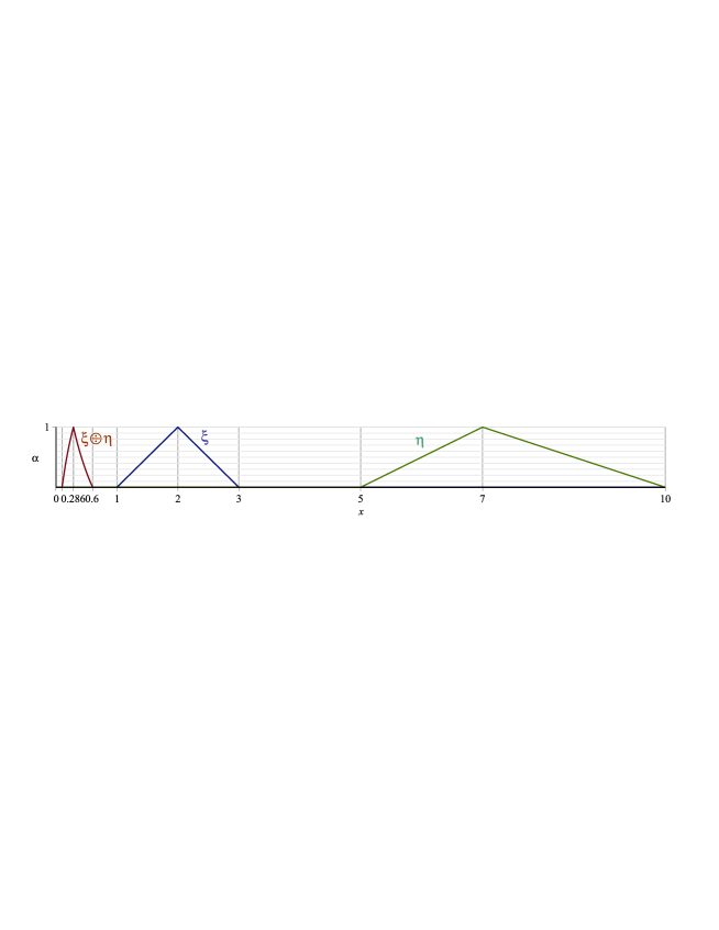
Figure 18. Fuzzy division of two triangle numbers

4. $\mathcal{F}_{c}(\mathbb{R})^{-1}$ - reversing the point of view

Especially in the case when fuzzy intervals are actively designed to model an economic situation to begin with as in management science, as opposed to being an expression of uncertainty in measurement of the outcome of an experiment in a natural science, it is obviously more natural and certainly more straightforward for computation to start with the right-hand sides of equations (2.2) and (2.3) as primary from the very outset.

This leads to the so-called parametric representation of fuzzy intervals as suggested by R. Goetschel and W. Voxmann in [2] and [3], and which has been predominant in the recent literature.

Therefore we propose to adopt the following definition, and associated terminology:

Definition 4.

We understand a fuzzy (generalized) interval

$$A^{*}\in[0,1]^{\mathbb{R}}\times[0,1]^{\mathbb{R}}$$

with fuzzy endpoints $a_{d}(\cdot),a_{u}(\cdot)$ to be an ordered pair of functions in shorthand denoted by $A^{*}:=[a_{d}(\cdot),a_{u}(\cdot)]$ such that:

• $a_{d}(\cdot):[0,1]\mapsto\mathbb{R}$ is increasing and left-continuous,

• $a_{u}(\cdot):[0,1]\mapsto\mathbb{R}$ is decreasing, right-continuous.

Furthermore we demand in consistence with Definition 2(2) and Remark 2.2:

• $\lim_{\alpha\to{0^{+}}}a_{d}(\alpha)=a_{d}(0),$

• $\lim_{\alpha\to{1^{-}}}a_{u}(\alpha)=a_{u}(1).$

Notation and Terminology:

• To distinguish real intervals $A$ from fuzzy intervals $A^{*}$ we use the starred form for the fuzzy interval.

• We as before call the (parameterizing) characterizing functions $a_{d}(\cdot)$, $a_{u}(\cdot)$ the fuzzy endpoints of the fuzzy interval $[a_{d},a_{u}]$ but use square brackets for the interval in parameterized form to distinguish it from the same interval in what we now might call the $x-$axis representation $\bigl{(}\overleftarrow{a_{d}}(\cdot),\overleftarrow{a_{u}}(\cdot)\bigr{)}.$

• We propose to denote $a_{d}(1)=\underline{a}$ and $a_{u}(1)=\overline{a}$ and refer to the real interval $A=[\underline{a},\overline{a}]$ as the (real) core (that is the real interval we are generalizing) of $A^{*}$.

• The support of the fuzzy interval $A^{*}$ in parametric form is $\operatorname{supp}{A^{*}}=[d,u]$ with $d=\alpha_{d}(0)$ and $u=a_{u}(0)$.

4.1. Arithmetic operations on $\mathcal{F}_{c}(\mathbb{R})^{-1}$

For two fuzzy intervals $A^{*}=[a_{d},a_{u}]$ and $B^{*}=[b_{d},b_{u}]$ all four arithmetic operations on $\mathcal{F}_{c}(\mathbb{R})^{-1}$ are then defined simply by:

(4.1) $$\begin{split}&A^{*}\circ B^{*}=\\ &\bigl{[}\min(a_{d}\circ b_{d},a_{d}\circ b_{u},a_{u}\circ b_{d},a_{u}\circ b_{u}),\max(a_{d}\circ b_{d},a_{d}\circ b_{u},a_{u}\circ b_{d},a_{u}\circ b_{u})\bigr{]}\end{split}$$

as in crisp interval arithmetic with “$\circ$” denoting any of the four operations: “$\oplus,\ominus,\odot,\oslash$”.

All comments and simplifications of section 3 apply with the appropriate modifications.

Example 9.

Real intervals $[\underline{a},\overline{a}]$ correspond to fuzzy endpoints

$a_{d}(\alpha)=\underline{a}\text{ for }\alpha\in[0,1]$ and

$a_{u}(\alpha)=\overline{a}\text{ for }\alpha\in[0,1].$

Example 10.

Fuzzy numbers are then fuzzy intervals in the sense above for the case the interval $[\underline{a},\overline{a}]$ is degenerated, that is $\underline{a}=\overline{a}=x_{0}$ for some $x_{0}\in\mathbb{R}$.

Example 11.

Triangle numbers $tr_{(l,m,r)}$ were characterized in section 1 by

(4.2) $$tr(x)=\begin{cases}tr_{l}(x)=\frac{x-l}{m-l}&\text{ for }x\in[l,m]\\ 1&\text{ for }x=m\\ tr_{r}(x)=\frac{r-x}{r-m}&\text{ for }x\in[m,r]\,.\end{cases}$$

We now write simply

(4.3) $$tr^{*}_{(d,x_{0},u)}(\alpha)=[\alpha(x_{0}-d)+d,u-\alpha(u-x_{0})],\quad\alpha\in[0,1]\,.$$

Rewriting in parametric representation our very first Example 1 in which we considered the two triangle numbers $tr_{1}=tr_{(1,2,3)}$ and $tr_{2}=tr_{(5,7,10)}$:

$$\begin{split}tr^{*}_{1}(\alpha)&=[\alpha(2-1)+1,3-\alpha(3-2)]=[\alpha+1,3-\alpha]\,,\\ tr^{*}_{2}(\alpha)&=[\alpha(7-5)+5,10-\alpha(10-7)]=[2\alpha+5,10-3\alpha].\end{split}$$

Then by (4.1), Remark 3.3 and Remark 3.5 we obtain

$$tr^{*}_{1}\oplus tr^{*}_{2} = \left[(\alpha+1)+(10-3\alpha),(3-\alpha)+(2\alpha+5)\right]=[10-2\alpha,8-3\alpha]\,,$$

$$tr^{*}_{1}\ominus tr^{*}_{2} = \left[(\alpha+1)-(2\alpha+5),(3-\alpha)-(10-3\alpha)\right]=[-\alpha-4,-7+2\alpha]\,,$$

$$tr^{*}_{1}\odot tr^{*}_{2} = \left[(\alpha+1)\cdot(2\alpha+5),(3-\alpha)\cdot(10-3\alpha)\right]\,,$$

$$tr^{*}_{1}\oslash tr^{*}_{2} = \left[\frac{\alpha+1}{10-3\alpha},\frac{3-\alpha}{2\alpha+5}\right].$$

very simply and straightforward, without having to go through the hassle of inverting and re-inverting.

To recapitulate:

The main motivation and advantage of this section’s approach is: By changing the point of view right from the start, when we set up a model and in doing so define a set of fuzzy intervals, the cumbersome procedure of (twice!) inverting normally un-invertible functions is avoided.

This is especially true when characterizing functions of mixed support are involved, and we close this section with some random impressions of various multiplied triangle numbers of mixed support, ($tr^{*}_{1}$: green, $tr^{*}_{2}$: blue, $tr^{*}_{1}\odot tr^{*}_{2}$: red) that have been rewritten as in Example 15:

4.2. Algebraic properties of the class $\mathcal{F}_{c}(\mathbb{R})$ (equivalently $\mathcal{F}_{c}(\mathbb{R})^{-1}$)

As was the case for $\mathcal{F}_{c}^{0}(\mathbb{R}^{+})$, $\mathcal{F}_{c}(\mathbb{R}^{+})$ we have associativity and commutativity.
Compared to sections 1 and 2 we gain subtraction and division (Division could have been introduced from the outset in section 1 by 3.9). We realize however that neither really constitutes an inverse operation in the group sense to the basic operations of addition and multiplication.

The distributive property of $\mathcal{F}_{c}^{0}(\mathbb{R}^{+})$, $\mathcal{F}_{c}(\mathbb{R}^{+})$ is lost. We only retain sub-distributivity in the sense that for every $\alpha\in[0,1]$ (that is for every $\alpha-$cut, at every $\alpha-$level) for three fuzzy intervals $[a_{d}(\alpha),a_{u}(\alpha)]$, $[b_{d}(\alpha),b_{u}(\alpha)]$ and $[c_{d}(\alpha),c_{u}(\alpha)]$,

(4.4) $$[a_{d},a_{u}]\odot\bigl{(}[b_{d},b_{u}]\oplus[c_{d},c_{u}]\bigr{)}\subseteq\bigl{(}[a_{d},a_{u}]\odot[b_{d},b_{u}]\bigr{)}\oplus\bigl{(}[a_{d},a_{u}]\odot[c_{d},c_{u}]\bigr{)}$$

holds as sets.

Graphically the above means that the graph of the left hand side of (4.4) lies entirely within the graph of the right hand side.

References

[1]
Lotfi A. Zadeh, (1965)
Fuzzy sets,
Inf. Control 8, 338-353.
[2] Goetschel, R., Voxman, W. (1983). Topological properties of fuzzy numbers. Fuzzy Sets and Systems, 10(13): 87-99.
[3] Goetschel, R., Voxman, W. (1986). Elementary fuzzy calculus. Fuzzy Sets and Systems, 18(1): 31-–43.