$GHZ$ state generation of three Josephson qubits in presence of bosonic baths

Abstract

We analyze an entangling protocol to generate tripartite Greenberger-Horne-Zeilinger states in a system consisting of three superconducting qubits with pairwise coupling. The dynamics of the open quantum system is investigated by taking into account the interaction of each qubit with an independent bosonic bath with an ohmic spectral structure. To this end a microscopic master equation is constructed and exactly solved. We find that the protocol here discussed is stable against decoherence and dissipation due to the presence of the external baths.

1 Introduction

Since its introduction, quantum entanglement has played a central role in foundational discussions of quantum mechanics. More recently due to the advent of new more applicative areas, like quantum information and communication fields, the concept of entanglement has attracted a renewed interest from the scientific community. Entangled quantum states have indeed proved to be essential resources both for quantum information processing and computational tasks. Also for this reason, in the last few years many efforts have been devoted to the design and the implementation, in very different physical areas, of schemes aimed at generating entangled states [1, 2, 3, 4, 5, 6, 7, 8, 9, 10, 11, 12]. In this context, in particular, superconductive qubits turned out to be promising candidates providing their scalability and the possibility of controlling and manipulating their quantum state in situ via external magnetic field and voltage pulses [13, 14, 15, 16].

The efficiency of solid state architectures, however, is unavoidably limited by decoherence and dissipation phenomena related to the presence of different noise sources partly stemming from control circuitry but also having microscopic origin. Thus, having as final target the realization of states characterized by prefixed quantum correlations, it is obviously important to estimate the effects of the coupling between the system considered and its surroundings.

Very recently Galiautdinov and Martinis [1] have presented a protocol suitable for generating maximally entangled states, namely $GHZ$ and $W$ states, of three Josephson qubits. The key idea on which their proposal is based, is that for implementing symmetric states, as the $GHZ$ and $W$ are, it is convenient to symmetrically control all the qubits in the system. In particular, making use of a triangular coupling interaction scheme and exploiting single qubit local rotations, they demonstrate the possibility of generating the desired state appropriately setting the interaction time between the qubits. In their analysis however, the authors considered the system as an ideal one, without taking into account in any way its unavoidable coupling with uncontrollable external degrees of freedom. In this paper, following the idea proposed in ref.[1], we investigate on the effects of the environment on the generation of $GHZ$ states. More in detail, we concentrate our attention on all the external degrees of freedom that can be effectively modelized as independent bosonic modes taking into account their presence from the very beginning. We moreover exploit the same triangular coupling mechanism envisaged in ref. [1] but we modify the single qubit rotation protocols with respect the ones of Galiautdinov and Martinis. Our analysis clearly prove that the scheme for generating GHZ states is stable enough against the noise sources we consider.

The paper is organized as follows: in section 2 we briefly discuss the key ingredients of the Galiautdinov and Martinis (G-M) procedure whereas in section 3 we propose a possible way to reduce the time required to generate the desired states. All the steps of the generation protocol are then investigated in section 4 supposing that each qubit of the system interacts with an independent bosonic bath. The last section is devoted to the discussion of the result we have obtained.

2 Galiautdinov - Martinis entangling protocol

In this section we briefly summarize the single step entangling protocol, proposed by Galiautdinov and Martinis in order to generate the three-qubits $GHZ$ states

$${|GHZ\rangle}=\frac{1}{\sqrt{2}}(\displaystyle{|000\rangle}+e^{i\varphi}\displaystyle{|111\rangle})$$ (1)

being $\displaystyle{|0\rangle}$ and $\displaystyle{|1\rangle}$ the ground and excited states of each qubit respectively. More in particular we review some aspects of the procedure that are of interest in the context of the present paper. The Hamiltonian model describing the physical system consisting of three Josephson qubits with pairwise coupling, is given by

$$H=\sum_{i=1}^{3}\Big{(}\frac{\omega}{2}\sigma_{z}^{i}+\frac{1}{2}[g(\sigma_{x}^{i}\sigma_{x}^{i+1}+\sigma_{y}^{i}\sigma_{y}^{i+1})+\tilde{g}\sigma_{z}^{i}\sigma_{z}^{i+1}]\Big{)}$$ (2)

with $\sigma_{k}^{4}=\sigma_{k}^{1}$ ($k=x,y,z$). Introducing the collective operators

$$\mathbf{S}=\sum_{j=1}^{3}\frac{\bm{\sigma}^{j}}{2}$$ (3)

we can rewrite equation (2) in the following more convenient form

$$H=\omega S_{z}+gS^{2}-(g-\tilde{g})S_{z}^{2}$$ (4)

within a constant term. Starting from equation (4) it is evident that the eigenstates of the system can be written as common eigenstates $\displaystyle{|s_{12},s,m\rangle}$ of the operators $S_{12}^{2}=\bigr{[}\frac{1}{2}(\bm{\sigma}^{1}+\bm{\sigma}^{2})\bigr{]}^{2}$, $S^{2}$ and $S_{z}$:

$$S_{12}^{2}\displaystyle{|s_{12},s,m\rangle} =s_{12}(s_{12}+1)\displaystyle{|s_{12},s,m\rangle}$$

$$S^{2}\displaystyle{|s_{12},s,m\rangle} =s(s+1)\displaystyle{|s_{12},s,m\rangle}$$ (5)

$$S_{z}\displaystyle{|s_{12},s,m\rangle} =m\displaystyle{|s_{12},s,m\rangle}$$

In particular it is immediate to convince oneself that the two states $\displaystyle{|000\rangle}\equiv\Bigl{|}s_{12}=1,s=\frac{3}{2},s_{z}=-\frac{3}{2}\Bigr{\rangle}$ and $\displaystyle{|111\rangle}\equiv\Bigl{|}s_{12}=1,s=\frac{3}{2},s_{z}=\frac{3}{2}\Bigr{\rangle}$ are eigenstates of $H$ correspondent to the eigenvalues $-\frac{3}{2}\omega+\frac{3}{4}(2g+3\tilde{g})$ and $\frac{3}{2}\omega+\frac{3}{4}(2g+3\tilde{g})$ respectively. In view of these considerations it is clear that, if at $t=0$ the three qubits are in their respective ground state, in order to guide the system toward the desired state (1) it becomes necessary to implement some local rotations before turning on the interaction mechanism described by equation (2). This is what Galiautdinov and Martinis do, making thus sure an initial condition having both $\displaystyle{|000\rangle}$ and $\displaystyle{|111\rangle}$ components. The entanglement is then performed by switching on, for an appropriate interval of time $t_{int}=\frac{\pi}{2(g-\tilde{g})}$, the interaction described by equation (2) and finally by realizing an additional single-qubit rotation. The scheme thus consists of three different steps: in the first and the third ones, the Josephson qubits are independent and are driven by external fields in order to appropriately rotate their state. In the second step instead the three qubits are coupled thus producing the desired entanglement among them.

3 Single-qubit rotations

As we have underlined in section 2, starting from the initial condition $\displaystyle{|000\rangle}$ the interaction mechanism described in equation (2) can be usefully exploited for generating $GHZ$ states of three qubits, only if local rotation operations are realized as first and final steps of the procedure. These two distinct operations of the protocol require a total time of realization $t_{13}=t_{1}+t_{3}$, which has to add to the length of the qubit interaction time $t_{int}=\frac{\pi}{2(g-\tilde{g})}$, if we wish to estimate the total duration of the generation scheme. Thus the choice of the physical mechanism able to perform appropriate single qubit rotations, could be usefully exploited to control the time required to generate the desired state starting from the state $\displaystyle{|000\rangle}$. This aspect is of particular interest especially when the presence of external degrees of freedom is not negligible. At the light of these considerations we have chosen rotation mechanisms different from the ones envisaged in ref.[1]. In particular we suppose that in the first, as well as in the last step of the scheme, whose duration is hereafter indicated by $t_{1}$ and $t_{3}$ respectively, the system of the three qubits is described by the following Hamiltonian

$$H_{rot}^{l}=\sum_{j=1}^{3}H_{rot}^{l}(j)\hskip 22.76228pt(l=I,III)$$ (6)

with

$$H_{rot}^{l}(j)=\frac{\omega}{2}\sigma_{z}^{j}+\frac{\omega}{2}\left(e^{i\beta_{l}}\sigma_{-}^{j}+\mathrm{h.c.}\right)$$ (7)

where

$$\beta_{I} =\pi\left(\frac{1}{\sqrt{2}}+1\right)$$ (8)

$$\beta_{III} =\pi\left(\frac{3+\sqrt{2}}{2}\right)+\pi\left(\frac{(3+\sqrt{3})\omega}{8(g-\tilde{g})}\right).$$

In ref. [17] is discussed in detail a possible way to realize hamiltonian model like the one given by equation (6) showing in particular that a full control of qubit rotations on the entire Bloch sphere can be achieved.

It is possible to prove that setting $t_{1}=t_{3}=\frac{\pi}{\sqrt{2}\omega}$, the sequence of the three steps leads to the desired $GHZ$ states when the interaction between the system of the three Josephson qubits and the external world may be neglected. After some calculation indeed it is possible to obtain that at $t=t_{1}$ the state of the system is given by

$$\displaystyle{|\psi(t_{1})\rangle}=\frac{1}{\sqrt{8}}\bigg{(}\displaystyle{|000\rangle}+\displaystyle{|111\rangle}e^{-\frac{3i\pi}{\sqrt{2}}}+\sqrt{3}\displaystyle{|W\rangle}e^{-\frac{i\pi}{\sqrt{2}}}+\sqrt{3}\displaystyle{|W^{\prime}\rangle}e^{-\sqrt{2}i\pi}\bigg{)}.$$ (9)

where

$${|W\rangle}=\frac{1}{\sqrt{3}}(\displaystyle{|100\rangle}+\displaystyle{|010\rangle}+\displaystyle{|001\rangle})$$ (10)

and

$${|W^{\prime}\rangle}=\frac{1}{\sqrt{3}}(\displaystyle{|011\rangle}+\displaystyle{|101\rangle}+\displaystyle{|110\rangle}).$$ (11)

At $t=t_{1}$ the interaction mechanism described by equation (2) is switched on for a time $t_{int}=\frac{\pi}{2(g-\tilde{g})}$. At the end of this second step the state of the system will be

$$\displaystyle{|\psi(t_{1}+t_{int})\rangle}= \frac{1}{\sqrt{8}}\bigg{(}\displaystyle{|000\rangle}+\displaystyle{|111\rangle}e^{-\frac{3i\pi}{2}\big{(}\frac{\omega}{g-\tilde{g}}+\sqrt{2}\big{)}}+$$

$$-\sqrt{3}\displaystyle{|W\rangle}e^{i\pi(\frac{(\sqrt{3}-3)\omega}{4(g-\tilde{g})}-\frac{\sqrt{2}}{2})}-\sqrt{3}\displaystyle{|W^{\prime}\rangle}e^{-i\pi(\frac{(\sqrt{3}+3)\omega}{4(g-\tilde{g})}+\sqrt{2})}\bigg{)}.$$

Thus the last step of the procedure described by $H_{rot}^{III}$, leads the system into the final state

$${|\psi(t_{1}+t_{int}+t_{3})\rangle}=\frac{1}{2}\bigg{[}(i+e^{i\alpha})\displaystyle{|000\rangle}+ie^{-i\theta}(i-e^{i\alpha})\displaystyle{|111\rangle}\bigg{]}$$ (13)

with

$$\alpha=\frac{3\pi\omega(\sqrt{3}-1)}{8(g-\tilde{g})}$$

$$\theta=\frac{3\pi\sqrt{2}}{2}+\frac{3\pi\omega(\sqrt{3}+3)}{8(g-\tilde{g})}.$$ (14)

Starting from equations (13) and (3) it is immediate to convince oneself that, if the condition

$$\frac{\omega}{g-\tilde{g}}=\frac{8k}{3(\sqrt{3}-1)}\hskip 22.76228ptk\in\mathbb{N}$$ (15)

is satisfied, the three Josephson qubits are left in the desired $GHZ$ state.
Thus we can say that the time required to generate the state (1) starting from the condition $\displaystyle{|000\rangle}$ can be estimated as

$$t_{tot}=t_{1}+t_{int}+t_{3}=\frac{\sqrt{2}\pi}{\omega}+\frac{\pi}{2(g-\tilde{g})}.$$ (16)

This value of $t_{tot}$ has to be compared with a time $t_{tot}=\frac{\pi}{\Omega}+\frac{\pi}{2(g-\tilde{g})}$, with $\Omega\ll\omega$ required if the procedure of Galiautdinov and Martinis is adopted. Starting indeed from the results presented in refs [1] and [18], it is possible to convince oneself that the proposal of Galiautdinov and Martinis requires that in the first an in the last step of the procedure the dynamics of each qubit is governed by the following Hamiltonian model

$$H_{GM}^{I,III}=\sum_{j}H_{GM}^{I,III}(j)$$ (17)

where

$$H_{GM}^{I,III}(j)=\frac{\omega}{2}\sigma_{z}^{j}+\Omega cos(\omega t+\phi_{I,III})\sigma_{x}^{j}$$ (18)

with $\Omega\ll\omega$ and $\phi_{I}=-\frac{\pi}{2}$ $\phi_{III}=0$.

Thus, changing the way to rotate the state of the three qubits during the first and the last step of the procedure, is possible to reduce the time required to generate the target state. As said before, this aspect is of particular relevance when the interaction of the system with the external world is not negligible. The price to pay anyway is that in our case, differently from the scheme of Galiautdinov and Martinis, three qubit GHZ states can be generated only if the condition given in equation (15) is satisfied. Generally speaking, indeed, at the end of the procedure, the three Josephson qubits are left in a linear superposition of the two states $\displaystyle{|000\rangle}$ and $\displaystyle{|111\rangle}$ with amplitudes $A_{000}=\frac{1}{2}(i+e^{i\alpha})$ and $A_{111}=\frac{i}{2}e^{-i\theta}(i-e^{i\alpha})$ respectively. It is important however, to stress that the condition (15) is compatible with typical values of the free frequency $\omega$, that generally speaking can be taken of the order of 10GHz, and with the values of the coupling constants $g$ and $\tilde{g}$, that reasonably can be assumed of the order of 1GHz and $10^{-1}$GHz respectively [19, 20, 21, 22]. On the other hand, condition (15) is not so mandatory as it appears, since we have verified that variations of ten percent in the ratio $\frac{\omega}{g-\tilde{g}}$ are still compatible with the requirement that $|A_{000}|^{2}\simeq|A_{111}|^{2}$.

4 Microscopic master equation derivation

In a realistic description of the scheme until now discussed we cannot neglect the presence of uncontrollable external degrees of freedom coupled to the three Josephson qubits that, generally speaking, affects in a bad way quantum state generation protocols. These degrees of freedom, that define the so-called environment, can have different physical origin and thus different descriptions. In this section we will focus our attention on all the external degrees of freedom describable as independent bosonic modes [23, 24, 25, 26, 27, 28, 29, 30, 31]. More in detail, we will suppose that during all the process each qubit is coupled to a bosonic bath and the three baths are independent.

The plausibility of this assumption can be tracked back to the fact that the three superconductive qubits are spatially separated so that it is reasonable to suppose that each of them is affected by sources of noise stemming from different parts of the superconductive circuit. In this section we review all the three steps of the procedure before discussed, analyzing the dynamics of the system by considering from the very beginning the interaction of each qubit with a bosonic bath. In order to do this we will construct and solve microscopic master equations in correspondence to the three different steps described in section 3 in which the generation scheme is structured. In each of the three steps the master equation will be derived in the Born - Markov and Rotating wave approximations [32]. We wish to stress at this point that the use of microscopic master equations instead of naiver and more popular phenomenological ones, becomes important particularly when structured reservoirs are considered [33].

4.1 First step: single-qubit rotation

Let us suppose that the three Josephson qubits are initially prepared in the ground state $\displaystyle{|000\rangle}$ and that the Hamiltonian describing the system in the first step of the procedure is given by equation (6) with $l=I$. Each qubit moreover is coupled to a bosonic bath and the three baths are independent. The Hamiltonian model describing the system in the first step can be thus written as [34]

$$H_{1}=H_{rot}^{I}+H_{B}+H_{int}\\$$ (19)

with

$$H_{B}\equiv H_{B}(1)+H_{B}(2)+H_{B}(3)=$$ (20)

$$= \sum_{k}\omega_{k}^{1}a_{k}^{1{\dagger}}a_{k}^{1}+\sum_{k}\omega_{k}^{2}a_{k}^{2{\dagger}}a_{k}^{2}+\sum_{k}\omega_{k}^{3}a_{k}^{3{\dagger}}a_{k}^{3}$$

and

$$H_{int}=\sigma_{x}^{1}\otimes\sum_{k}g_{k}^{1}(a_{k}^{1}+ a_{k}^{1{\dagger}})+\sigma_{x}^{2}\otimes\sum_{k}g_{k}^{2}(a_{k}^{2}+a_{k}^{2{\dagger}})+$$

$$+\sigma_{x}^{3}\otimes\sum_{k}g_{k}^{3}(a_{k}^{3}+a_{k}^{3{\dagger}}).$$

Exploiting standard procedure [32] we now derive the microscopic master equation suitable to describe the dynamics of the three qubits system. Taking into account the fact that the qubits, as well as the baths, are, in this case, independent, it is enough to construct and solve the master equation correspondent to a single superconductive qubit. Indicating by $\rho_{j}(t)$ the density matrix of the $j$-th $(j=1,2,3)$ qubit, it is possible to prove that during the first step we have

$$\dot{\rho}_{j}(t)=-i[H_{rot}^{I}(j),\rho_{j}(t)]+$$

$$\gamma_{1}(\omega_{1})\biggr{(}A_{j}(\omega_{1})\rho_{j}(t)A_{j}^{\dagger}(\omega_{1})-\frac{1}{2}\big{\{}A_{j}^{\dagger}(\omega_{1})A_{j}(\omega_{1}),\rho_{j}(t)\big{\}}\biggr{)}+$$ (22)

$$\gamma_{1}(\omega_{2})\biggr{(}A_{j}(\omega_{2})\rho_{j}(t)A_{j}^{\dagger}(\omega_{2})-\frac{1}{2}\big{\{}A_{j}^{\dagger}(\omega_{2})A_{j}(\omega_{2}),\rho_{j}(t)\big{\}}\biggr{)}$$

where the Bohr frequencies are respectively $\omega_{1}=\sqrt{2}\omega$ and $\omega_{2}=0$ whereas the correspondent operators, describing the jumps between the eigenstates $\displaystyle{|\psi_{\pm}\epsilon\rangle}_{j}$ ($\epsilon=\frac{\omega}{\sqrt{2}}$), of the Hamiltonian $H_{rot}^{I}(j)$, are given by

$$A_{j}(\omega_{1}) \equiv\displaystyle{|\psi_{-\epsilon}\rangle}_{jj}\displaystyle{\langle\psi_{-\epsilon}|}\sigma_{x}^{j}\displaystyle{|\psi_{\epsilon}\rangle}_{jj}\displaystyle{\langle\psi_{\epsilon}|}=$$

$$=\bigg{(}\frac{1}{\sqrt{2}}\cos{\frac{\pi}{\sqrt{2}}}-i\sin{\frac{\pi}{\sqrt{2}}}\bigg{)}\displaystyle{|\psi_{-\epsilon}\rangle}_{jj}\displaystyle{\langle\psi_{\epsilon}|}$$

$$A_{j}(\omega_{2}) \equiv\displaystyle{|\psi_{-\epsilon}\rangle}_{jj}\displaystyle{\langle\psi_{-\epsilon}|}\sigma_{x}^{j}\displaystyle{|\psi_{-\epsilon}\rangle}_{jj}\displaystyle{\langle\psi_{-\epsilon}|}+$$

$$+\displaystyle{|\psi_{\epsilon}\rangle}_{jj}\displaystyle{\langle\psi_{\epsilon}|}\sigma_{x}^{j}\displaystyle{|\psi_{\epsilon}\rangle}_{jj}\displaystyle{\langle\psi_{\epsilon}|}=$$

$$=\frac{1}{\sqrt{2}}\cos{\frac{\pi}{\sqrt{2}}}\bigg{(}\displaystyle{|\psi_{-\epsilon}\rangle}_{jj}\displaystyle{\langle\psi_{-\epsilon}|}-\displaystyle{|\psi_{\epsilon}\rangle}_{jj}\displaystyle{\langle\psi_{\epsilon}|}\bigg{)}$$

with

$$\displaystyle{|\psi_{\epsilon}\rangle}_{j}=\frac{1}{2}\left[\sqrt{2+\sqrt{2}}e^{-i\beta_{I}}\displaystyle{|1\rangle}_{j}+\sqrt{2-\sqrt{2}}\displaystyle{|0\rangle}_{j}\right]$$ (24)

$$\displaystyle{|\psi_{-\epsilon}\rangle}_{j}=\frac{1}{2}\left[\sqrt{2-\sqrt{2}}e^{-i\beta_{I}}\displaystyle{|1\rangle}_{j}-\sqrt{2+\sqrt{2}}\displaystyle{|0\rangle}_{j}\right].$$

Concerning the decay rates $\gamma_{1}(\omega_{1})$ and $\gamma_{1}(\omega_{2})$ appearing in equation (4.1), we will fix their numerical value in the next section where we explicitly give the spectral properties of the baths.

4.2 Second step: entangling procedure

As we have previously discussed, the next step requires that the three qubits interact among them through the coupling mechanism described by equation (4). In addition each qubit interacts with a bosonic bath. Thus the Hamiltonian describing the total system in this second step can be written as

$$H_{2}=H+H_{B}+H_{int}.$$ (25)

The master equation for the density matrix of the three qubits during the second step can be written in the form

$$\dot{\rho}(t)= -i[H,\rho(t)]+$$

$$+\sum_{j=1}^{3}\sum_{k=1}^{8}\gamma_{2}(\omega_{k})\biggr{(}A_{j}(\omega_{k})\rho(t)A_{j}^{\dagger}(\omega_{k})-\frac{1}{2}\big{\{}A_{j}^{\dagger}(\omega_{k})A_{j}(\omega_{k}),\rho(t)\big{\}}\biggr{)}$$

where the Bohr frequencies are the following

$$\omega_{1,3} =\frac{3-\sqrt{3}}{2}\omega\pm 2(g-\tilde{g})$$

$$\omega_{2,4} =\frac{3}{2}\omega\mp(g+2\tilde{g})$$

$$\omega_{5} =\sqrt{3}\omega$$ (27)

$$\omega_{6,7} =\frac{\sqrt{3}}{2}\omega\pm 3g$$

$$\omega_{8} =0$$

whereas the jump operators between the eigenstates of the Hamiltonian (4) are given for convenience in appendix B. We wish to underline that equation (4.2) does not contain mixed terms of the form $A_{j}(\omega_{k})\rho(t)A_{j^{\prime}}^{\dagger}(\omega_{k})-\frac{1}{2}\big{\{}A_{j}^{\dagger}(\omega_{k})A_{j^{\prime}}(\omega_{k}),\rho(t)\big{\}}$ with $j\neq j^{\prime}$ in view of the fact that the three bosonic baths are independent.

We have solved the master equation (4.2), considering as initial condition the solution of the master equation (4.1) obtained in the previous paragraph at $t=t_{1}$ . More in detail, taking into account the fact that the ideal scheme provides a dynamics confined in the subspace generated by the states $\displaystyle{|000\rangle}$, $\displaystyle{|111\rangle}$, $\displaystyle{|W\rangle}$ and $\displaystyle{|W^{\prime}\rangle}$, we have focused our attention on the projection of $\rho(t)$ on this subspace. It is possible indeed to prove that the neglected subspace will be at the most populated with a probability not exceeding the 3%.

4.3 Third step: local rotations

To complete the analysis of the GHZ state generation procedure in presence of noise, we have to construct the microscopic master equation describing the system in the last step of the scheme. Actually it can be immediately deduced from the master equation derived in the first step simply substituting $\beta_{I}$ with $\beta_{III}$ in the eigenstates $\displaystyle{|\psi_{\pm\epsilon}\rangle}$ appearing in the jump operators. However, in this case it is more convenient to write the jump operators exploiting the basis

$$\displaystyle{|\widetilde{000}\rangle}=T\displaystyle{|000\rangle}$$

$$\displaystyle{|\widetilde{111}\rangle}=T\displaystyle{|111\rangle}$$

$$\displaystyle{|\widetilde{W}\rangle}=T\displaystyle{|W\rangle}=\frac{1}{\sqrt{3}}T(\displaystyle{|100\rangle}+\displaystyle{|010\rangle}+\displaystyle{|001\rangle})$$

$$\displaystyle{|\widetilde{W^{\prime}}\rangle}=T\displaystyle{|W^{\prime}\rangle}=\frac{1}{\sqrt{3}}T(\displaystyle{|011\rangle}+\displaystyle{|101\rangle}+\displaystyle{|110\rangle})$$

$$\displaystyle{|\widetilde{\psi_{1}}\rangle}=T\displaystyle{|\psi_{1}\rangle}=\frac{1}{\sqrt{2}}T(\displaystyle{|100\rangle}-\displaystyle{|010\rangle})$$ (28)

$$\displaystyle{|\widetilde{\psi_{1}^{\prime}}\rangle}=T\displaystyle{|\psi_{1}^{\prime}\rangle}=\frac{1}{\sqrt{2}}T(\displaystyle{|011\rangle}-\displaystyle{|101\rangle})$$

$$\displaystyle{|\widetilde{\psi_{2}}\rangle}=T\displaystyle{|\psi_{2}\rangle}=\frac{1}{\sqrt{6}}T(\displaystyle{|100\rangle}+\displaystyle{|010\rangle}-2\displaystyle{|001\rangle})$$

$$\displaystyle{|\widetilde{\psi_{2}^{\prime}}\rangle}=T\displaystyle{|\psi_{2}^{\prime}\rangle}=\frac{1}{\sqrt{6}}T(\displaystyle{|011\rangle}+\displaystyle{|101\rangle}-2\displaystyle{|110\rangle}).$$

instead of the standard one. In this new basis the unitary operator $T$ can be represented as

$$T=\frac{\sqrt{2+\sqrt{2}}}{8}\left(\begin{array}[]{ccc}B_{1}&&0\\ &B_{2}&\\ 0&&B_{3}\\ \end{array}\right)$$ (32)

with

$$B_{1}= {\scriptsize\left(\begin{array}[]{cccc}-(2+\sqrt{2})&-(4-3\sqrt{2})&\sqrt{6}&-\sqrt{3}(2-\sqrt{2})\\ -(4-3\sqrt{2})e^{-3i\beta_{III}}&(2+\sqrt{2})e^{-3i\beta_{III}}&\sqrt{3}(2-\sqrt{2})e^{-3i\beta_{III}}&\sqrt{6}e^{-3i\beta_{III}}\\ \sqrt{6}e^{-i\beta_{III}}&\sqrt{3}(2-\sqrt{2})e^{-i\beta_{III}}&(3\sqrt{2}-2)e^{-i\beta_{III}}&-(4-\sqrt{2})e^{-i\beta_{III}}\\ -\sqrt{3}(2-\sqrt{2})e^{-2i\beta_{III}}&\sqrt{6}e^{-2i\beta_{III}}&-(4-\sqrt{2})e^{-2i\beta_{III}}&-(3\sqrt{2}-2)e^{-2i\beta_{III}}\\ \end{array}\right)}$$ (37)

$$B_{2}= \left(\begin{array}[]{cc}4e^{-i\beta_{III}}&4(\sqrt{2}-1)e^{-i\beta_{III}}\\ 4(\sqrt{2}-1)e^{-2i\beta_{III}}&-4e^{-2i\beta_{III}}\\ \end{array}\right)$$ (40)

$$B_{3}= \left(\begin{array}[]{cc}4e^{-i\beta_{III}}&4(\sqrt{2}-1)e^{-i\beta_{III}}\\ 4(\sqrt{2}-1)e^{-2i\beta_{III}}&-4e^{-2i\beta_{III}}\\ \end{array}\right)$$ (43)

It is possible to demonstrate that in this case the master equation can be written as

$$\dot{\rho}(t)= -i[H_{rot}^{III},\rho(t)]+$$

$$+\sum_{j=1}^{3}\sum_{i=1}^{2}\gamma_{3}(\omega_{i})\biggr{(}A_{j}(\omega_{i})\rho(t)A_{j}^{\dagger}(\omega_{i})-\frac{1}{2}\big{\{}A_{j}^{\dagger}(\omega_{i})A_{j}(\omega_{i}),\rho(t)\big{\}}\biggr{)}$$

where the Bohr frequencies are the same as the ones in the first step whereas the jump operators $A_{j}(\omega_{i})$ between the eigenstates of the Hamiltonian $H_{rot}^{III}$ are for convenience given in the appendix C.

5 Results and conclusions

Having at disposal the microscopic master equations (4.1), (4.2) and (4.3), describing the dynamics of the three-qubit system, we have found the density matrix $\rho(t_{tot})$ of the system at the time instant $t_{tot}=t_{1}+t_{int}+t_{3}$, supposing that at $t=0$ the initial condition was $\displaystyle{|\psi(0)\rangle}=\displaystyle{|000\rangle}$. Moreover, we have assumed that all the three baths were characterized by the same spectral density given in particular by the ohmic one

$$\gamma(\omega)=\Bigg{\{}\begin{array}[]{c}\gamma_{0}\;\;\;\;\;\omega=0\\ \alpha\omega\;\;\;\;\;\omega\neq 0\end{array}$$ (45)

where $\gamma_{0}$ is introduced in order to take into account a non zero decay rate for $\omega=0$.

To quantify the effects of the bosonic baths we can consider the fidelity F

$$\emph{F}=Tr\{\rho_{exp}\rho(t_{tot})\}$$ (46)

that gives an idea of the difference existing between the density matrix $\rho_{exp}$, obtained when the interaction with the three baths is neglected, and the density matrix $\rho(t_{tot})$. The results we have obtained are for convenience given in figure 1 where we plot F as a function of the ratio $\omega/g$ assigning to the parameters $\gamma_{0}$ and $\alpha$ physically reasonable values. In particular we have chosen $\gamma_{0}=\alpha=10^{-3}$ [20, 19, 21, 22] .

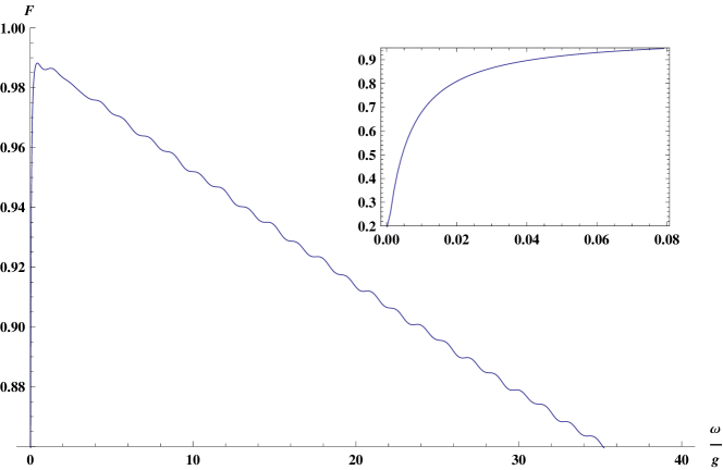
Figure 1: Fidelity $F$ as a function of $\omega/g$ when we assume that all the three baths were characterized by the same ohmic spectral density given in (45) with $\gamma_{0}=\alpha=10^{-3}$ and the parameters assume the values $\tilde{g}/g=0.1$. The inset shows the Fidelity for values $0<\omega/g<0.08$.

As we can see, at least for $\omega\lesssim 20g$ the presence of bosonic baths at zero temperature does not affect in a significative way the dynamics of the system during the different steps of the procedure, being the fidelity not less that 0.90. One should expect that the fidelity $F$ is a monotonically decreasing function of $\omega/g$. The model we have used for the decay rate (see eq.(45), however, is discontinuous for zero frequency because we want to consider also possible dephasing channels. In view of this discontinuity one is not allowed to perform the limit $\omega/g$ tending to zero in the fidelity. Anyway this is not a problem in view of the fact that for $\omega=0$ our scheme is meaningless since in this limit no rotations are performed. Moreover, as the inset in figure 1 shows, the increase of $F$ is rapid with respect to $\omega/g$.
Let us now observe that increasing of an order of magnitude the bath decay rates, the fidelity $F$ remains experimentally significative as shown in figure 2.

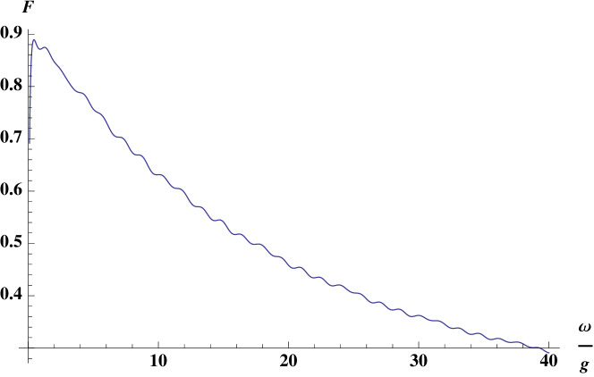
Figure 2: Fidelity $F$ as a function of $\omega/g$ when we assume that all the three baths were characterized by the same ohmic spectral density given in (45) with $\gamma_{0}=\alpha=10^{-2}$ and the parameters assume the values $\tilde{g}/g=0.1$.

Both figures make evident that the presence of the three independent bosonic baths does not affect in a dramatic way the results reached under the hypothesis of perfect isolation.

We are however interested to the generation of GHZ states as given in equation (1), which, as we have previously seen, can be obtained only if the condition (15) is satisfied. Thus it is of interest for us to analyze the fidelity $\emph{F}_{GHZ}$ defined as

$$\emph{F}_{GHZ}=Tr\{\displaystyle{|GHZ\rangle}\displaystyle{\langle GHZ|}\rho(t_{tot})\}$$ (47)

and reported in figures 3 and 4 as a function of the ratio $\omega/g$.

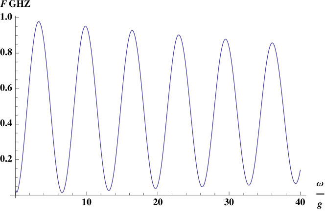
Figure 3: Fidelity $F_{GHZ}$ as a function of $\omega/g$ when we assume that all the three baths were characterized by the same ohmic spectral density given in (45) with $\gamma_{0}=\alpha=10^{-3}$ and the parameters assume the values $\tilde{g}/g=0.1$. To evaluate $F_{GHZ}$ we put $\varphi=\frac{3\pi}{2}(\sqrt{3}+\frac{(3+\sqrt{3})}{4}\frac{\omega}{g-\tilde{g}})$ for the GHZ state in equation (47).

Figure 3 is obtained in correspondence of bath decay rates generally reported in literature as realistic ones [20, 19, 21, 22] whereas the results reported in figure 4 are obtained supposing worse conditions. As expected, the fidelity $\emph{F}_{GHZ}$ shows maxima in correspondence to values of $\omega/g$ such to satisfy condition (15). The value of such maxima moreover decreases increasing the ratio $\omega/g$. This circumstance is in turn related to the fact that the decay rates appearing in the master equations (4.1), (4.2) and (4.3), are increasing functions of $\omega$. However, also considering the worst case we may conclude that it is possible to choose an interval of values of the ratio $\omega/g$ in correspondence of which $\emph{F}_{GHZ}$ is greater than 0.7. On the other hand for experimentally reasonable values of the decay rates $\gamma_{0}$ and $\alpha$ we can obtain values of $\emph{F}_{GHZ}$ greater than 0.9 also fixing $\omega/g$ in different intervals, see figure 3. Notwithstanding these values of the fidelity are less than the fault tolerance threshold, they are surely of interest in the context of generation schemes of quantum states having assigned properties.

We thus may conclude that the scheme before discussed to generate GHZ states (1) is robust enough with respect to the presence of noise sources describable as independent bosonic baths.

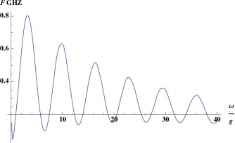
Figure 4: Fidelity $F_{GHZ}$ as a function of $\omega/g$ when we assume that all the three baths were characterized by the same ohmic spectral density given in (45) with $\gamma_{0}=\alpha=10^{-2}$ and the parameters assume the values $\tilde{g}/g=0.1$. To evaluate $F_{GHZ}$ we put $\varphi=\frac{3\pi}{2}(\sqrt{3}+\frac{(3+\sqrt{3})}{4}\frac{\omega}{g-\tilde{g}})$ for the GHZ state in equation (47).

6 Appendix A

The eigenstates of the Hamiltonian given in (4) can be written as common eigenstates $\displaystyle{|s_{12},s,m\rangle}$ of the operators $S_{12}^{2}=\bigr{[}\frac{1}{2}(\bm{\sigma}^{1}+\bm{\sigma}^{2})\bigr{]}^{2}$, $S^{2}$ and $S_{z}$ and can be cast in the form

$$\Bigl{|}1,\frac{3}{2},-\frac{3}{2}\Bigr{\rangle}=\displaystyle{|000\rangle}$$

$$\Bigl{|}1,\frac{3}{2},\frac{3}{2}\Bigr{\rangle}=\displaystyle{|111\rangle}$$

$$\Bigl{|}1,\frac{3}{2},-\frac{1}{2}\Bigr{\rangle}=\frac{1}{\sqrt{3}}(\displaystyle{|100\rangle}+\displaystyle{|010\rangle}+\displaystyle{|001\rangle})\equiv\displaystyle{|W\rangle}$$

$$\Bigl{|}1,\frac{3}{2},\frac{1}{2}\Bigr{\rangle}=\frac{1}{\sqrt{3}}(\displaystyle{|011\rangle}+\displaystyle{|101\rangle}+\displaystyle{|110\rangle})\equiv\displaystyle{|W^{\prime}\rangle}$$

$$\Bigl{|}0,\frac{1}{2},-\frac{1}{2}\Bigr{\rangle}=\frac{1}{\sqrt{2}}(\displaystyle{|100\rangle}-\displaystyle{|010\rangle})\equiv=\displaystyle{|\psi_{1}\rangle}$$

$$\Bigl{|}0,\frac{1}{2},\frac{1}{2}\Bigr{\rangle}=\frac{1}{\sqrt{2}}(\displaystyle{|011\rangle}-\displaystyle{|101\rangle})\equiv\displaystyle{|\psi_{1}^{\prime}\rangle}$$

$$\Bigl{|}1,\frac{1}{2},-\frac{1}{2}\Bigr{\rangle}=\frac{1}{\sqrt{6}}(\displaystyle{|100\rangle}+\displaystyle{|010\rangle}-2\displaystyle{|001\rangle})\equiv\displaystyle{|\psi_{2}\rangle}$$

$$\Bigl{|}1,\frac{1}{2},\frac{1}{2}\Bigr{\rangle}=\frac{1}{\sqrt{6}}(\displaystyle{|011\rangle}+\displaystyle{|101\rangle}-2\displaystyle{|110\rangle})\equiv\displaystyle{|\psi_{2}^{\prime}\rangle}.$$

The correspondent eigenvalues are given by

$$E_{\displaystyle{|000\rangle}}=-\frac{3}{2}(\omega-\tilde{g})$$

$$E_{\displaystyle{|111\rangle}}=\frac{3}{2}(\omega+\tilde{g})$$

$$E_{\displaystyle{|W\rangle}}=-\frac{1}{2}(\sqrt{3}\omega-4g+\tilde{g})$$ (49)

$$E_{\displaystyle{|W^{\prime}\rangle}}=\frac{1}{2}(\sqrt{3}\omega+4g-\tilde{g})$$

$$E_{\displaystyle{|\psi_{r}\rangle}}=-(g+\frac{\tilde{g}}{2})\;\;\;\;\mathrm{for}\;\;\;r=1,1^{\prime},2,2^{\prime}$$

7 Appendix B

The Bohr frequencies of the system in the second step are given in (4.2) and the correspondent jump operators are respectively

$$A_{j}(\omega_{1})= \frac{1}{\sqrt{3}}\displaystyle{|000\rangle}\displaystyle{\langle W|}\;\;\;\;j=1,2,3$$

$$A_{j}(\omega_{2})= (-1)^{j+1}\frac{1}{\sqrt{2}}\displaystyle{|000\rangle}\displaystyle{\langle\psi_{1}|}+\frac{1}{\sqrt{6}}\displaystyle{|000\rangle}\displaystyle{\langle\psi_{2}|}\;\;\;j=1,2$$

$$A_{3}(\omega_{2})= -\sqrt{\frac{2}{3}}\displaystyle{|000\rangle}\displaystyle{\langle\psi_{2}|}$$

$$A_{j}(\omega_{3})= \frac{1}{\sqrt{3}}\displaystyle{|W^{\prime}\rangle}\displaystyle{\langle 111|}\;\;\;j=1,2,3$$

$$A_{j}(\omega_{4})= (-1)^{j+1}\frac{1}{\sqrt{2}}\displaystyle{|\psi_{1}^{\prime}\rangle}\displaystyle{\langle 111|}+\frac{1}{\sqrt{6}}\displaystyle{|\psi_{2}^{\prime}\rangle}\displaystyle{\langle 111|}\;\;\;j=1,2$$

$$A_{3}(\omega_{4})= -\sqrt{\frac{2}{3}}\displaystyle{|\psi_{2}^{\prime}\rangle}\displaystyle{\langle 111|}$$

$$A_{j}(\omega_{5})= \frac{2}{3}\displaystyle{|W\rangle}\displaystyle{\langle W^{\prime}|}\;\;\;j=1,2,3$$

$$A_{j}(\omega_{6})= (-1)^{j}\frac{1}{\sqrt{6}}\displaystyle{|W\rangle}\displaystyle{\langle\psi_{1}^{\prime}|}-\frac{1}{3\sqrt{2}}\displaystyle{|W\rangle}\displaystyle{\langle\psi_{2}^{\prime}|}\;\;\;j=1,2$$ (50)

$$A_{3}(\omega_{6})= \frac{\sqrt{2}}{3}\displaystyle{|W\rangle}\displaystyle{\langle\psi_{2}^{\prime}|}$$

$$A_{j}(\omega_{7})= -\frac{1}{\sqrt{6}}\displaystyle{|\psi_{1}\rangle}\displaystyle{\langle W^{\prime}|}-\frac{1}{3\sqrt{2}}\displaystyle{|\psi_{2}\rangle}\displaystyle{\langle W^{\prime}|}\;\;\;j=1,2$$

$$A_{3}(\omega_{7})= \frac{\sqrt{2}}{3}\displaystyle{|\psi_{2}\rangle}\displaystyle{\langle W^{\prime}|}$$

$$A_{j}(\omega_{8})= (-1)^{j+1}\frac{1}{\sqrt{3}}(\displaystyle{|\psi_{1}\rangle}\displaystyle{\langle\psi_{2}^{\prime}|}+\displaystyle{|\psi_{1}^{\prime}\rangle}\displaystyle{\langle\psi_{2}|}+\displaystyle{|\psi_{2}\rangle}\displaystyle{\langle\psi_{1}^{\prime}|}+$$

$$+\displaystyle{|\psi_{2}^{\prime}\rangle}\displaystyle{\langle\psi_{1}|})-\frac{2}{3}(\displaystyle{|\psi_{2}\rangle}\displaystyle{\langle\psi_{2}^{\prime}|}+\displaystyle{|\psi_{2}^{\prime}\rangle}\displaystyle{\langle\psi_{2}|})\;\;\;j=1,2$$

$$A_{3}(\omega_{8})= -(\displaystyle{|\psi_{1}\rangle}\displaystyle{\langle\psi_{1}^{\prime}|}+\displaystyle{|\psi_{1}^{\prime}\rangle}\displaystyle{\langle\psi_{1}|})+\frac{1}{3}(\displaystyle{|\psi_{2}\rangle}\displaystyle{\langle\psi_{2}^{\prime}|}+$$

$$\displaystyle{|\psi_{2}^{\prime}\rangle}\displaystyle{\langle\psi_{2}|}).$$

8 Appendix C

As far as the third step it is useful to rewrite the jump operators of the first step in the basis $\displaystyle{|\widetilde{000}\rangle}$, $\displaystyle{|\widetilde{111}\rangle}$, $\displaystyle{|\widetilde{W}\rangle}$, $\displaystyle{|\widetilde{W^{\prime}}\rangle}$, $\displaystyle{|\widetilde{\psi_{1}}\rangle}$, $\displaystyle{|\widetilde{\psi_{1}^{\prime}}\rangle}$, $\displaystyle{|\widetilde{\psi_{2}}\rangle}$ and $\displaystyle{|\widetilde{\psi_{2}^{\prime}}\rangle}$

$$A_{j}(\omega_{1})= -\frac{1}{2\sqrt{3}}\bigg{[}\big{(}\cos{\beta}+i\sqrt{2}\sin{\beta}\big{)}\big{(}\sqrt{2}\displaystyle{|\widetilde{W}\rangle}\displaystyle{\langle\widetilde{000}|}+$$

$$+\sqrt{3}\displaystyle{|\widetilde{\psi_{1}}\rangle}\displaystyle{\langle\widetilde{000}|}+\displaystyle{|\widetilde{\psi_{2}}\rangle}\displaystyle{\langle\widetilde{000}|}\big{)}+\big{(}\cos{\beta}-i\sqrt{2}\sin{\beta}\big{)}\times$$

$$\times\big{(}\sqrt{2}\displaystyle{|\widetilde{W^{\prime}}\rangle}\displaystyle{\langle\widetilde{111}|}+\sqrt{3}\displaystyle{|\widetilde{\psi_{1}^{\prime}}\rangle}\displaystyle{\langle\widetilde{111}|}+\displaystyle{|\widetilde{\psi_{2}^{\prime}}\rangle}\displaystyle{\langle\widetilde{111}|}\big{)}\bigg{]}\;\;\;j=1,2$$

$$A_{3}(\omega_{1})= -\frac{1}{\sqrt{6}}\bigg{[}\big{(}\cos{\beta}+i\sqrt{2}\sin{\beta}\big{)}\big{(}\displaystyle{|\widetilde{W}\rangle}\displaystyle{\langle\widetilde{000}|}+$$ (51)

$$-\sqrt{2}\displaystyle{|\widetilde{\psi_{2}}\rangle}\displaystyle{\langle\widetilde{000}|}\big{)}+\big{(}\cos{\beta}-i\sqrt{2}\sin{\beta}\big{)}\big{(}\displaystyle{|\widetilde{W^{\prime}}\rangle}\displaystyle{\langle\widetilde{111}|}+$$

$$-\sqrt{2}\displaystyle{|\widetilde{\psi_{2}^{\prime}}\rangle}\displaystyle{\langle\widetilde{111}|}\big{)}\bigg{]}$$

$$A_{j}(\omega_{2})= -\frac{\cos{\beta}}{3\sqrt{2}}\bigg{[}3\displaystyle{|\widetilde{000}\rangle}\displaystyle{\langle\widetilde{000}|}-3\displaystyle{|\widetilde{111}\rangle}\displaystyle{\langle\widetilde{111}|}+\displaystyle{|\widetilde{W}\rangle}\displaystyle{\langle\widetilde{W}|}+$$

$$-\displaystyle{|\widetilde{W^{\prime}}\rangle}\displaystyle{\langle\widetilde{W^{\prime}}|}+2\displaystyle{|\widetilde{\psi_{2}}\rangle}\displaystyle{\langle\widetilde{\psi_{2}}|}-2\displaystyle{|\widetilde{\psi_{2}^{\prime}}\rangle}\displaystyle{\langle\widetilde{\psi_{2}^{\prime}}|}\bigg{]}\;\;\;j=1,2$$

$$A_{3}(\omega_{2})= -\frac{\cos{\beta}}{3\sqrt{2}}\bigg{[}3\displaystyle{|\widetilde{000}\rangle}\displaystyle{\langle\widetilde{000}|}-3\displaystyle{|\widetilde{111}\rangle}\displaystyle{\langle\widetilde{111}|}+$$

$$+\displaystyle{|\widetilde{W}\rangle}\displaystyle{\langle\widetilde{W}|}-\displaystyle{|\widetilde{W^{\prime}}\rangle}\displaystyle{\langle\widetilde{W^{\prime}}|}+3\displaystyle{|\widetilde{\psi_{1}}\rangle}\displaystyle{\langle\widetilde{\psi_{1}}|}+$$

$$-3\displaystyle{|\widetilde{\psi_{1}^{\prime}}\rangle}\displaystyle{\langle\widetilde{\psi_{1}^{\prime}}|}+2\displaystyle{|\widetilde{\psi_{2}}\rangle}\displaystyle{\langle\widetilde{\psi_{2}}|}-2\displaystyle{|\widetilde{\psi_{2}^{\prime}}\rangle}\displaystyle{\langle\widetilde{\psi_{2}^{\prime}}|}\bigg{]}.$$

References

- [1] A. Galiautdinov and J. Martinis, Phys. Rev. A 78, 010305(R) (2008)
- [2] R. Migliore, K. Yuasa, H. Nakazato and A. Messina, Phys. Rev. B 74, 104503 (2006)
- [3] L. F. Wei, Y. X. Liu and F. Nori, Phys. Rev. Lett. 96, 246803 (2006)
- [4] S. Matsuo, S. Ashhab, T. Fujii, F. Nori, K. Nagai and N. Hatakenaka, J. Phys. Soc. Japan 76, 054802 (2007)
- [5] R. Migliore, K. Yuasa, M. Guccione, H. Nakazato and A. Messina, Phys. Rev. B 76, 052501 (2007)
- [6] M. Neeley, R. C. Bialczak, M. Lenander, E. Lucero, M. Mariantoni, A. D. O’Connell, D. Sank, H. Wang, M. Weides, J. Wenner, Y. Yin, T. Yamamoto, A. N. Cleland and J. M. Martinis, Nature 467, 570 (2010)
- [7] L. DiCarlo, M. D. Reed, L. Sun, B. R. Johnson, J. M. Chow, J. M. Gambetta, L. Frunzio, S. M. Girvin, M. H. Devoret and R. Schoelkopf, Nature 467, 574 (2010)
- [8] R. Migliore, M. Scala, A. Napoli, K. Yuasa, H. Nakazato and A. Messina, J. Phys. B: At. Mol. Opt. Phys. 44, 075503 (2011)
- [9] M. Wallquist, K. Hammerer, P. Zoller, C. Genes, M. Ludwig, F. Marquardt, P. Treutlein, J. Ye and H. J. Kimble, Phys. Rev. A 81, 023816 (2010)
- [10] L. M. Duan and H. J. Kimble, Phys. Rev. Lett. 92, 127902, (2004)
- [11] H. Kampermann, D. Bruß, X. Peng and D. Suter, Phys. Rev. A 81, 040304(R) (2010)
- [12] C. Ospelkaus, U. Warring, Y. Colombe, K. R. Brown, J. M. Amini, D. Leibfried and D. J. Wineland, arXiv.org:quant-ph/1104.3573 (2011)
- [13] M. H. Devoret, A. Wallraff and J. M. Martinis, ArXiv.org:cond-mat/0411174 (2004)
- [14] L. S. Levitov, T. P. Orlando, J. B. Majer, J. E. Mooij arXiv.org:cond-mat/0108266 (2001)
- [15] S. H. W. van der Ploeg, A. Izmalkov, A. Maassen van den Brink, U. H”ubner, M. Grajcar, E. Il’ichev, H. -G. Meyer and A. M. Zagoskin, Phys. Rev. Lett. 98, 057004 (2007)
- [16] C. Cosmelli, M. G. Castellano, F. Chiarello, R. Leoni, D. Simeone, G. Torrioli and P. Carelli, arXiv.org:cond-mat/0403690 (2004)
- [17] L. Chirolli and G. Burkard, Phys. Rev. B 74, 174510 (2006)
- [18] M. R. Geller, E. J. Pritchett, A. Galiautdinov and J. M. Martinis, Phys. Rev. A 81, 012320 (2010)
- [19] J. Q. You and F. Nori, Phys. Today 58, 42 (2005)
- [20] Y. Makhlin, G. Schön and A. Shnirman, Rev. Mod. Phys. 73, 357 (2001)
- [21] M. H. Devoret and J. Martinis, Quantum Inf. Process 3, 163 (2004)
- [22] M. Scala, R. Migliore, A. Napoli and L. L. Sánchez-Soto, Eur. Phyis. J. D. 61, 199 (2011)
- [23] N. P. Oxtoby, Á. Rivas, S. F. Huelga and R. Fazio, New J. Phys. 11, 063028 (2009)
- [24] A. Shnirman, G. Schön, I. Martin and Y. Makhlin, Phys. Rev. Lett. 94, 127002 (2005)
- [25] E. Paladino, L. Faoro, G. Falci and R. Fazio, Phys. Rev. Lett. 88, 228304 (2002)
- [26] Y. M. Galperin, B. L. Altshuler, J. Bergli and D. V. Shantsev, Phys. Rev. Lett. 96, 097009 (2006)
- [27] L. Faoro, J. Bergli, B. L. Altshuler and Y. M. Galperin, Phys. Rev. Lett. 95, 046805 (2005)
- [28] A. Grishin, I. V. Yurkevich and I. V. Lerner, Phys. Rev. B 72, 060509 (2005)
- [29] J. Schriefl, Y. Makhlin, A. Shnirman and G. Schön, New J. Phys. 8, 1 (2006)
- [30] B. Abel and F. Marquardt, Phys. Rev. B 78, 201302 (2008)
- [31] L. Faoro and L. B. Ioffe, Phys. Rev. Lett. 100, 227005 (2008)
- [32] H. -P. Breuer and F. Petruccione, The Theory of Open Quantum Systems, Oxford University Press, Oxford (2002)
- [33] R. Migliore, M. Scala, A. Napoli, K. Yuasa, H. Nakazato and A. Messina, J. Phys. B: At. Mol. Opt. Phys. 44, 075503 (2011)
- [34] M. Scala, R. Migliore and A. Messina, J.Phys. A: Math. Theor. 41, 435304 (2008)