A framework towards understanding mesoscopic phenomena: Emergent unpredictability, symmetry breaking and dynamics across scales
Abstract
By integrating four lines of thoughts: symmetry breaking originally advanced by Anderson, bifurcation from nonlinear dynamical systems, Landau’s phenomenological theory of phase transition, and the mechanism of emergent rare events first studied by Kramers, we introduce a possible framework for understanding mesoscopic dynamics that links () fast microscopic (lower level) motions, () movements within each basin-of-attraction at the mid-level, and () higher-level rare transitions between neighboring basins, which have slow rates that decrease exponentially with the size of the system. In this mesoscopic framework, the fast dynamics is represented by a rapidly varying stochastic process and the mid-level by a nonlinear dynamics. Multiple attractors arise as emergent properties of the nonlinear systems. The interplay between the stochastic element and nonlinearity, the essence of Kramers’ theory, leads to successive jump-like transitions among different basins. We argue each transition is a dynamic symmetry breaking, with the potential of exhibiting Thom-Zeeman catastrophe as well as phase transition with the breakdown of ergodicity (e.g., cell differentiation). The slow-time dynamics of the nonlinear mesoscopic system is not deterministic, rather it is a discrete stochastic jump process. The existence of these discrete states and the Markov transitions among them are both emergent phenomena. This emergent stochastic jump dynamics then serves as the stochastic element for the nonlinear dynamics of a higher level aggregates on an even larger spatial and slower time scales (e.g., evolution). This description captures the hierarchical structure outlined by Anderson and illustrates two distinct types of limit of a mesoscopic dynamics: A long-time ensemble thermodynamics in terms of time followed by the size of the system , and a short-time trajectory steady state with followed by . With these limits, symmetry breaking and cusp catastrophe are two perspectives of the same mesoscopic system on different time scales.
keywords:
catastrophe , Kramers’ theory , many-body physics , mesoscopic scale , metastability , nonlinear bifurcation , rare events , stochastic physics , thermodynamic limit1 Introduction
There is a growing trend in using protein dynamics with heterogeneous interacting atoms, either as a metaphore or as a mathematical representation, for understanding complex biological organisms such as single cells and even tumor tissues [1, 2, 3, 4]. Kinetic steady state is one of the fundamental concepts in chemical and biochemical reaction systems. Indeed, the notion of attractors has become increasingly relevant in studying cell differentiation and its fate determination, and cancer non-genetic heterogeneity [4, 5, 6, 7, 8, 9, 10, 11]. Painted in a broad stroke, dynamics with dissipation usually predicts a convergence of systems with different initial state. How can such a picture be consistent, then, with an increasing diversity and complexity as expected from living biological organisms according to Darwin’s theory?
In addition to a landscape perspective [12, 13, 14, 15, 16, 17, 18] that can be made very precise even for a large class of nonequilibrium systems in terms of a generalized Gibbs function, complex systems such as macromolecules, cells, and even biological organisms also share other important characteristics. The notion of symmetry breaking has been considered by many thinkers as a fundamental mechanism for generating complexity [19, 20, 21, 22, 23]. At the core of this idea are two elements: () a singular point in the phase space of a nonlinear dynamical system where the future of the dynamics is truly unpredictable [24] and () a noise “too small to be taken into account of by a finite being” [25] with a lack of detailed information for physical origin, or too erratic to be fully comprehended by a rational person.
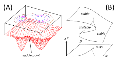
In modern mathematical theory of nonlinear dynamics, () is known as a “saddle point”: if a system is located precisely at the point and the dynamics is absolutely deterministic, then it will remain there forever. However, any infinitesimal perturbation will lead the system away towards somewhere else. (Being precise, the perturbation has to have a component along unstable manifold. Physically, a perturbation exactly restricted on a stable manifold is nearly impossible.) More importantly, depending upon a particular perturbation, there are in fact many possible outcomes, or fates, which are seemingly chosen by chance. In textbooks illustrations, this is usually drawn as a “double well potential” with an “energy barrier” in between, see Fig. 1, left pannel. Chemists have termed the saddle point a “transition state” [26].
What is the fundamental origin of ()? For a macromolecule immersed in an aqueous solution, fluctuations are well understood in terms of atoms at finite temperature [27]: They are too erratic to be meaningfully represented by deterministic mathematics due to the lack of detailed, or simply too much, information of the motions of the individuals in the system. Therefore, Fourier, Boltzmann, Einstein, Gibbs, Onsager, and Kramers, together with many pioneers in the physics of matter, have advanced a probabilistic description of the states and dynamics of a complex, many-body system. (The probability in quantum physics has a fundamentally different origin. Quantum dynamics is conservative while dynamics in thermal physics is dissipative. See [28, 29, 30, 31] for more discussions.)
The modern statistical theory of matter developed by physicists and chemists explains the macroscopic, deterministic world in terms of the erratic, stochastic dynamics of atoms and molecules. Its fundamental insight lies at the mathematical law of large numbers (LLN): The same law that gives Las Vegas casinos more confidence in their profitability if more people are willing to gamble. However, another lesson from this story has not been told often enough: An individual gambler with a nearly infinite amount of time and money will win a jackpot, if the rule of the game never changes. Furthermore, there is actually no logical causality between a person and a winning event. (If anything, the logical causality is in the mechanical movements of a slot machine; and why and when a machine is picked due to physiological and psychological processes [20] of an individual gambler.) Individual winning event is unpredictable. What is certain is that it will occur with probability 1 on any given machine and the time to the occurrence is an exponentially distributed memoryless random variable [32].
The successes of the LLN in classical statistical mechanics have created an impression that any system consisting of a large number of atoms and/or molecules can be describable by deterministic mathematics: Stochastic behaviors are averaged out. This impression is rather misleading, especially when dealing with nonlinear dynamics of a system consisting of large number of individuals. In fact, as we shall show, stochasticity does not disappear in a wide class of systems that have multistability, or the potential for phase transitions. Here, stochasticities simply manifest themselves as rare events on a longer time scale; larger a system, longer the time. Then on an even longer time scale, numerous rare events constitute another deterministic, continuous dynamics: A single molecule conformational transition is a rare event in Kramers’ theory, but they are the basis for the deterministic kinetics of a chemical reaction system based on the Law of Mass Action [33, 34, 35, 36].
2 Hierarchical Organization at Different Levels and Different Time Scales
Indeed, P.W. Anderson stated that [19] “At each level of complexity entirely new properties appear, and the understanding of the new behaviors requires research which I think is as fundamental in its nature as any other.” He went on to list a series of different levels of complexity: few-body (elementary particle) physics, many-body physics, chemistry, molecular biology, …, physiology, psychology, and social sciences. The elementary entities of each level in the hierarchy obey the dynamic laws of a level lower, and at each level an entirely new laws, concepts, and generalizations emerge, and different treatment and theories are necessary. Our mesoscopic stochastic framework fits this hierarchy. This hierarchy shares many features with the organizational hierarchy among protein conformational sub-states advanced by H. Frauenfelder and coworkers [12, 2, 35]: Going downward, a protein consists of secondary structural motifs, which consists of amino acids, which consists of atoms, etc. Going upward, a cell consists of a large number of macromolecules, and a tissue consists of a large population of cells, etc. As an example, a recent study used contact geometry ideas to examine how to move complex descriptions of a system from one level to another [37]. In our framework, we expect coarse-grained descriptions emerge from the collective dynamics.
The chemical reaction theory, together with protein science, serve as a paradigm for stochastic, mesoscopic complexity [1, 2, 17, 22, 35, 36, 38]. Consider a chemical transformation in an aqueous solution. The conceptual framework for such a reaction developed by Kramers [33] is now accepted as the theoretical foundation of chemical reactions in condensed phase. In fact, a chemical reaction theory involves three levels in Anderson’s hierarchy: () few-body physics detailing the collisions of a few water molecules (H2O) with a few atoms within reacting molecules; () many-body physics concerning molecules , and in a sea of solvent molecules; and () chemistry whose elementary events are discrete chemical reactions such as . In () one is concerned with collisions leading to high-frequency vibrations; () is primarily interested in the mechanism and process of how and collide, interact and formation of occurs in terms of the atoms in the molecules with vibrations and diffusion, while in () the actual chemical reaction is represented by a single second-order rate constant for a discrete transition. Fig. 2A uses a schematics to illustrate this hierachy.
Kramers’ theory predicts that these different levels also translate to different time scales [1]: At the time scale of a molecular reaction, the process in () is so fast that it can be essentially treated as infinitely rapid fluctuating dynamics with certain appropriate statistics. The time scale for processes in () is of course determined by the energy and force in the molecular system which Kramers called “a field of force”, and the outcome of the theory is a discrete event of an elementary chemical reaction whose time scale, sec., is almost infinite on the time scale of (), sec. Kramers’ mathematical theory is one of the first that reveals an interplay between“chance” and “necessity” [41, 42, 43, 44].
Now for a cellular biochemist who is interested in a metabolic system with many biochemical species, the individual on the sub-sec scale is just part of fluctuations. He/she is interested in the dynamics of how various concentrations of metabolites change with time. By using Law of Mass Action, steady states of the biochemical reaction system which can be reached on the order of seconds, can be predicted. Then on an even longer time scale, recent studies on phenotypic switching point to the stochastic transitions from one biochemical steady state to another in a single cell, on the time scale of sec. Again, to , is essentially infinite. Figs. 2B again shows an illustrative schematics.
One of the deepest concepts developed by chemists in connection to chemical reactions is the notion of “transition state” [26, 45]. We see that it is at the very transition state the dynamic of a symmetry breaking occurs in molecular systems. If a molecular system is infinitely large, then this symmetry breaking is static: the chance of Kramers’ barrier crossing could take the time as long as the age of the universe. This is the symmetry breaking picture of Anderson [19]. However, a macromolecule such as a protein can in fact jump among its different conformational states on the time scale observable in a laboratory [2, 27, 35] and exhibits successive dynamic symmetry breaking [20]. In this latter case, a discrete-state stochastic description of the dynamics in term of a Markov jump process is most appropriate [18, 46, 47]. As differential equation approach to classical dynamics, Markov approach to stochastic dynamics is very general. Even certain processes with long memory can be mathematically transformed into a Markovian representation.
A unavoidable mathematical issue is at the heart of any theory of mesoscopic systems. As Anderson pointed out in [19] that “It is only as the nucleus is considered to be a many-body system — in what is often called the limit — that such emergent behavior is rigorous definable.” The importance of taking thermodynamic limit in a mathematical theory of phase transition goes back to Kramers in 1936 [48]. The thermodynamic limit according to textbooks on equilibrium physics of matters is to take the time first and then systems size afterward. In fact, the limit never appeared since equilibrium is assumed at the onset. On the other hand, for nonlinear dynamic behavior in a macroscopic system, one often takes the limit first for finite . In fact, nonlinear, emergent dynamic behavior of a complex system can only be rigorously defined with [18], followed with fluctuation analysis with finite . Our framework is explicitely concerned with the order of these two limits [49]. In reality, both limits are simple idealizations. Still, each limiting procedure has it validity on an appropriate time scale: relaxations within a basin of attraction and inter-attractor stochastic jumps.
3 Nonlinear bistability, bifurcation, and phase transition
In the mathematical theory of deterministic nonlinear dynamics, symmetry breaking is intimately related to the problem of saddle-node bifurcation [50]. In fact, the theory of saddle-node bifurcation and its topological representation, known as catastrophe theory, is exactly a symmetry breaking problem viewed in a relatively short time scale.
This section should be followed closely with Fig. 3 at side. It is essentially a mathematics exercise, with an explicit example given in the Appendix. For broader audiences, however, we choose to carry out the discussion using verbal narratives as much as possible. Let us consider an ordinary differential equation (ODE) for 1-d , with two parameters and . In other words, for each pair of , there is an ODE. Let us further assume that for some values of the ODE has only a single stable steady state (fixed point), and for other parameter values there are three steady states, two stable and , and one unstable in between: . Note the s are functions of and ; in fact, all the s irrespective of , or are roots of . This argebraic equation defines a surface shown in Fig. 1B. When a piece of paper is gently folded, the multiple steady states as functions of and form a multi-layer surface in 3-d.
In classical van der Waals gas problem, the variable is equilibrium volume of a box of gas, and are temperature and pressure. In a biochemical phosphorylation feedback system, is the fraction of phosphorylated protein, and are the kinase activity and ATP phosphorylation potential [51, 52]. The equation is known as an “equation of state” in van der Waals theory, and an “equation of phosphorylation-dephosphorylation switch” for signaling module [53] .
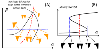
In Fig. 1B, projecting the three layers to the plane for the two parameters, topologist René Thom had the deep insight that the region has to have a wedged shape with a cusp as shown in Fig. 1B, also in Fig. 3A [54]. Now if you keep constant and vary acorss the wedged region starting from far left, as illustrated by the dashed blue line in Fig. 3A, the number of steady states changes from 1, to 2 to 3, and back to 2 and 1. This is shown in Fig. 3B. The black -shaped curve is a “bifurcation diagram” which shows the position of steady state(s) as a smooth function of (with a given ).
At the blue vertical lines in Fig. 3B, the phenomena of changing number of steady states are called saddle-node bifurcation. For small and large values of , the system has only a single steady state (fixed point). The blue dashed lines mark the critical values at which there is a sudden appearance or disappearance of a pair of stable and unstable steady states. The pair “bursts out of blue”; thus acquired the name of blue sky bifurcation [50]. One of the extensively studied examples of this type of behavior in biochemistry is forced molecular dissociation leading to non-covalent bond rupture [55].
So far, we have discribed how bifurcation arises in nonlinear, deterministic systems with bistability. A deterministic nonlinear approach is usually valid for macroscopic systems. From a mesoscopic perspective, this means all our above discussion starts with a system without fluctuation. More precisely, when one studies a mesoscopic molecular system, the numbers of individuals of various species in a system and the volume of the system, are usually specified. The ODE perspective is for infinitely large system, i.e., introducing “concentration” , and then mathematically taking to obtain a “macroscopic limiting behabior” in terms of the nonlinear dynamics for . Then in the limit of , multiple attractors is revealed. Different initial conditions will leads to different steady states. Because of this procedure, the transition between two fixed points, the most important consequence of fluctuations, is not possible in the deterministic analysis. There is a breakdown of ergodicity.
This is not the thermodynamic limit which requires a true equilibration among all different attractors. In fact, the most important information missing in the ODE analysis is the relative weights for different attractors. This comes from analysis based on probability and stochastic processes. A finite-size correction naturally introduces stochasticity. Depending upon the chosen representation for a system, a finite-size mesoscopic model can be a discrete or continuous stochastic process. For example, the dynamic equation for a stochastic concentration can be characterized by where represents the size of the dynamical system and represents a Brownian motion fluctuation. One notices that if , the dynamics is reduced to the above “macroscopic limit”.
To study the true thermodynamic limit, one lets first in a stochastic model followed by . This way, an initial value independent (i.e., ergodic) probability distribution across all attractors emerges. The mathematical theory for this type of stochastic differential equation (i.e., nonlinear Langevin equation) shows that the stationary density has the form [56]:
| (1) |
in which is a normalizationm factor. Furthermore, has local minima at and and a maximum at . This means the probability distribution peaks at and . It it the extrema of function that match the fixed points of . The behavior of the deterministic dynamics is closely related to the modal values of the finite, mesoscopic system rather the mean value [57].
The shapes of , the “landscapes” [9, 15, 16, 58, 59, 60, 61, 62], for different and are shown in Fig. 3A and B. For each there is a . Along the dashed blue line in Fig. 3A, the corresponding s are illustrated in orange, as well as the black shapes shown below the curve in 3B. When changing horizontally in 3A, the landscape for bistability develops a bias for one of the minima. Outside the wedged region, one of the minima disappears all together.
Note that Eq. 1 is obtained by letting while keeping finite. Now different phenomenon arises if one lets in (1): The distribution will concentrate at the global minimum of with probability 1! Even though a system can be bistable or multistable, a metastable state, i.e., the non-global local minimum of , has zero probability in the limit of , if one allows the system to truly equilibrate.
Therefore as predicted by the LLN, generically there is a unique steady state for a bistable (or multistable) system in the true thermodynamic limit, except at a critical when the two minima are precisely equal , shown in Fig. 1B, and the dashed red curve in Fig. 1A.(It is also clear that if the correlation in such a system at were short-ranged, then there would be infinite number of “identical, independent subsystem”, which would imply LLN being again valid. Thus, the violation of LLN at dictates an infinitely long, non-exponential decay correlation in the system.) For each given value, there exists an .
Therefore, in the limit of followed by , i.e., in the true thermodynamic limit, the -shaped curve in Fig. 3B is no more; only a discontinuous jump at , marked by the red dashed vertical line. This is a reminiscent of the Maxwell construction [63] for the van der Waals theory of non-ideal gas. Similarly, in Fig. 3A the wedge is no longer relevant; only the dashed red curve which should abruptly terminates at the cusp. This is known as a first-order phase transition line.
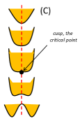
Now let us focus on the cusp in Fig. 3A. Moving along the red curve inside the wedged region, the landscape changes from symmetric bistable with two equal minima to a monostable single minimum, when passing the cusp. This is magnified in Fig. 3C. It is L.D. Landau’s second-order phase transition [64]. In nonlinear dynamical systems theory, crossing the cusp constitutes a robust pitchfork bifurcation [50].
Therefore, a kind of symmetry and symmetry breaking emerge in the simple bistable nonlinear system with stochasticity, i.e., a complex mesoscopic system. Table 1 summaries the discussions above: In the left column, with , followed by ; in the middle column while holding finite, and the right column gives the true thermodynamic limit as followed by .
How is this “mathematical” description of bifurcation and phase transition related to the traditional physics of matters? Thermodynamic description of a system neglects all time scales that are too long to be of interests, then assumes that all the remaining time scales reach an ergodic stationarity. We emphasize this point since strictly speaking there are always slow processes in reality. For example, there is a slow rate of peptide hydrolysis in an aqueous solution for any protein molecule. But this effect is usually neglected, rightly, in the thermodynamic theory of protein conformational transitions. Also, according to Newton’s third law, there is always a consequence at the origin that generates a force. For example a magnet that induces supercurrent in a type II superconductor decays slowly. Deterministic nonlinear dynamic description of a system, on the other hand, considers interesting dynamics in the medium time range: Different initial conditions will lead to different steady states. The true equilibration among different steady states, however, is out of reach in a deterministic description. A mesoscopic system can exhibit rich behavior precisely because both scenarios are accessible and they even interact [17, 38, 42, 63].
A mean-field treatment in the classical physics usually entails deriving a relation among “mean values” by neglecting fluctuations. Therefore, it corresponds to first. Thus often it is incapable of reaching the ergodic thermodynamic limit. Furthermore, the cusp is precisely the critical point in Landau’s phenomenological phase transition of ferromagnet in terms of free energy with [65]. This is the symmetry breaking picture generally discussed in the theory of phase transition. Changing and correspond to changing and in the above . The essence of Landau’s theory is a bistable system with stochasticity (noise) [42].
Yang and Lee have established a general mathematical origin for phase transition [66, 67]. They have shown that the mathematical non-analyticity, a necessary feature of any rigorous phase transition theory, is related to a zero of a partition function moving from complex plane onto real axis in the limit (Recall that the free energy is the logarithm of a partition function.) It has been demonstrated recently that this same mathematical description applies to any bistable system with stochastic elements [51, 52], including mesoscopic biochemical system with bistability. Therefore, the notion of phase transition, together with key concepts such as symmetry breaking and the perspective of “true thermodynamic limit” have a broad applicability to systems exhibiting phenomena as catastrophe, rupture, and hysteresis [55]. It is a complementary description of bistability in the presence of stochasticity.
The notion of symmetry breaking used in [19, 20] is intimately related to bifurcation. While bifurcation of a ground state in solid-state and particle physics is due to a symmetry in a Hamiltonian [2], nonlinear complex systems have symmetries, with canonical forms, at their bifurcation points [50]. However, the existence of multistability and attractors is often an emergent phenomenon itself. Our above discussions illustrate that with stochasticity, bifurcations in the true thermodynamic limit exhibit phase transitions — a probability distribution has certain symmetry; a realization by a particular system breaks the symmetry. In fact the pitchfork bifurcation is a necessary part of a catastrophe phenomenon.
4 Emergent discrete stochastic dynamics in nonlinear systems with multiple attractors
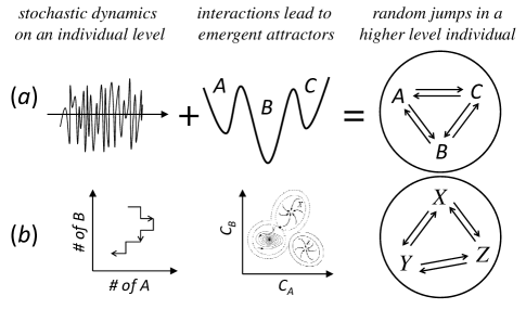
The forgoing discussion focused on systems with bistability. For a highly nonlinear, complex system with stochastic elements, there could be a large number of attractors. Therefore, on a time scale much longer than the deterministic dynamics that occurs within each basin of attraction, inter-attractor dynamics can be represented as a Markov jump process among a set of discrete states. This is an insight one learns from macromolecular dynamics like those of a protein: Kramers’ theory accounts the transition rates, usually with an exponentially distributed waiting time, between each pair of “conformational states”; but the dynamics of an enzyme is usually represented by chemical kinetics which represents the conformational states in discrete terms. More interestingly, in recent years the Delbrück-Gillespie approach to nonlinear biochemical reaction systems treats each elementary chemical reaction in a mesoscopic volume as a stochastic process, and derives endogenous phenotypic “cellular states” [3, 8, 16, 17, 58, 59, 61] and cellular evolutionary dynamics [6, 47]. Robustness of a cellular state and punctuated equilibrium in state transitions are necessary consequences of this dynamics description.
The time scales, short or long, are defined by the Kramers’ theory for a barrier-crossing process. It is tempting to suggest that complexity at a mesoscopic scale originates from a system with the size at which both the deterministic, converging dynamics on a short-time and the stochastic, diverging dynamics on a long-time are accessible to an observer [2, 22]. We stress that the stochastic fluctuations on the very fast time scale yield the divergent behavior of stochastic jumps out of the basins of attraction on a very long time scale [2]. Conversely, interactions between dynamics at these different time scales lead to slow dynamics modulating the fast motions with possible eddy current [3, 11, 17, 68, 69, 70, 71, 72]. A stochastic system in general moves toward states with higher probability, exhibiting a form of contingency [2], or adaptation [73, 74]. In enzyme kinetics, this is the origin of dynamic disorder [35]. It is also illuminating to point out that an ab inito computation of the emergent stochastic transitions from the detailed dynamics can range from a highly challenging task to practically infeasible [75]: In protein folding, this is only accomplished very recently for a single transition of biochemical significance based on atomic-level molecular dynamics [76].
Let us reiterate: The insights from the present discussion which departs from the LLN perspective is that stochasticity does not completely disappear in a reasonably large, nonlinear mesoscopic system. Rather, it manifests itself as a stochastic jump process on a much longer time scale among a set of discrete states, as has been shown in Fig. 2A and B. These discrete states are attractors of an interacting nonlinear dynamical system. These discrete states are determined by the behavior and interactions among individuals within the system; yet their existence, locations, and transition times are completely non-trivial. They are emergent properties. Well-known examples are cooperativity in equilibrium physics and feedbacks in biological networks [57]. In the former, cooperativity leads to crystallization; and in the latter nonequilibrium systems, feedbacks lead to self-organization. The nature of emergent phenomena is a consequence of nonlinear interactions between individuals [24, 42, 75].
The emergent stochastic jump dynamics of an individual, of course, becomes the stochastic elements for a higher level population system in a larger space with longer time. In this fashion, Anderson’s hierarchy moves up level by level with the nonlinear, stochastic dynamic framework [38]. This is again illustrated in Fig. 2. Recall the example of a single biological cell as a mesoscopic chemical reaction system where this hierachy has already been appreciated [1]: Boltzmann started the tradition of treating molecular collisions as stochastic elements in a kinetic theory. Kramers has shown that the discrete chemical reaction can be described as Brownian motion in a force field [33, 40]. Supported by the recent experimental advances in single-molecule chemistry and biophysics [27], Delbrück-Gillespie’s theoretical approach to chemical reactions considers each chemical reaction as a stochastic jump, and derives “states” and “dynamics” of cell-size biochemical reaction systems [6, 16, 17, 47, 60, 61].
Continuing with this perspective, the question of whether epigenetic phenotypic states at a cellular level is a part of intrinsic biochemical dynamics or an external, environmentally induced phenomenon can be addressed using a mesoscopic dynamic approach [6, 8, 16, 17, 57, 58]. Epigenetic switching could indeed be viewed as a “phase transition” in mesoscopic biochemical systems [17, 51, 52, 62]. Phase transition that might play a possible role in the emergence of life itself, as suggested recently in [77], should be understood as such.
5 Conclusions
The mathematical concept of thermodynamic limit is defined as an infinitely large system reaches its infinitely long-time limit, where the long-time has to be sufficient to overcome all the exponentially small barrier crossing probabilities. Therefore, it is immediately clear that there are two competing limits for time and systems size, and the order of taking these limits matters. Complex behavior arises when these two limits are not exchangeable due to non-uniform convergence [78]. As we have discussed, a real thermodynamic limit, which takes first, is simple. A mesoscopic system is messy — When Anderson talked about [19], there are in fact two possibilities: finite time dynamics requires taking it before , and thermodynamics requires taking it after : The latter produces a simpler picture of the world with universality, and the former produces a much more complex picture of a world with diversity.
The present discussion focuses on the emergence of discrete transitions between different dynamic basins. While we have not explicitly discussed system with spatial characteristics, we believe a large part of the discussions is applicable to stochastic reaction-diffusion systems [79, 80, 81, 82]. Recent work also points to the important phenomena associated with time symmetry breaking in nonequilibrium steady state of mesoscopic systems [16, 17, 44, 60, 83, 84, 85, 86]. A deeper understanding toward the relationships among different forms of symmetry breaking in space, time, and dynamics remain to be elucidated [21, 87].
In physics, the notion of mesoscopics often refers to dynamics such as conductance fluctuations in small size devices. In the present work we see the scope of “mesocopic phenomena” to be much broader: It can also cover many other interesting behavior including biochemical cells with self-organizations [47, 83]. In fact, it is the description in terms of stochastic nonlinear dynamics, incorporating both chance and necessity [41], that gives the “middle way” [22] a unique yet universal characteristics [15, 16, 17, 42, 44, 47, 60, 86]. This is one of the most fundamental insights of J.W. Gibbs, and the contribution of chemical science to the theory of complexity [1].
Acknowledgments
The authors thank S. A. Kauffman, A. J. Leggett, and P. G. Wolynes for helpful discussions, and NSF and NSFC for financial supports.
Table 1: Terminologies and Phenomena in Infinite-time Dynamics1
| Deterministic2 | Stochastic3,4 | |
|---|---|---|
| basin of attraction | landscape well | |
| global landscape minimum, | ||
| stable fixed points | landscape minima | all local minima have zero |
| (attractors) | probability | |
| unstable fixed point | landscape maxima | |
| (repellers) | ||
| out-of-blue saddle- | emergence of a pair of | n/a |
| node bifurcation | local min max | |
| bi-stability wedged | double-well region | wedged region collapses |
| region | into a coexistence line, | |
| Maxwell construction | order phase transition | |
| n/a | for two equal minima | |
| cusp | two equal minima | critical point |
| at the boundary of | ||
| pitchfork bifurcation | the wedged region | order phase transition |
1 n/a means a phenomenon has no correspondence, and significance, in this setting.
2 Deterministic means one takes first to obtained an ODE for , i.e., macroscopic limit, followed by to obtain steady states (attractors) of the determinstic nonlinear dynamics, starting with different initial values.
3 Stochastic dynamic with very large but finite size () has a proper probability density for its stationary process (i.e., while holding ): where is a landscape.
4 A true thermodynamic limit takes the results in the middle column, followed by . Because is normalized, the limit has a singular support, with probability 1 concentrated on the global minimum of .
 |
 |
|
References
- [1] P.G. Wolynes, Chemical reaction dynamics in complex molecular systems. In Complex Systems (SFI Studies in the Sciences of Complexity) Stein, D. ed., Addison-Wesley Longman Pub., pp. 355–387(1989).
- [2] H. Frauenfelder, and P.G. Wolynes, Biomolecules: where the physics of complexity and simplicity meet. Phys Today 47(Feb), 58–64(1994).
- [3] M. Sasai, and P.G. Wolynes, Stochastic gene expression as a many body problem. Proc. Natl. Acad. Sci. USA 100, 2374–2379(2003).
- [4] S. Kauffman, Differentiation of Malignant to Benign Cells. J. Theor. Biol. 31, 429-451 (1971).
- [5] R.A. Gatenby and T. L. Vincent, An evolutionary model of carcinogenesis Cancer Res. 63, 6212–6220. (2003).
- [6] J. Wang, K. Zhang, L. Xu, and E.K. Wang, Quantifying the Waddington landscape and biological paths for development and differentiation. Proc. Natl. Acad. Sci. USA 108, 8257–8262(2011).
- [7] S. Huang, I. Ernberg, and S. Kauffman, Cancer attractors: A systems view of tumors from a gene network dynamics and developmental perspective. Semin. Cell Dev. Biol. 20, 869–876 (2009).
- [8] P. Ao, D. Galas, L. Hood, and X. Zhu, Cancer as robust intrinsic state of endogenous molecular-cellular network shaped by evolution. Med. Hypoth. 70, 678–684(2008).
- [9] C.H. Li, and J. Wang, Quantifying the underlying landscape and paths of cancer. J. R. Soc. Inter. 11, 20140774(2014).
- [10] C.H. Li, J. Wang, Quantifying the Landscape for Development and Cancer from a Core Cancer Stem Cell Circuit. Cancer Res. 75, 2607–2618 (2015).
- [11] C. Chen, and J. Wang, A physical mechanism of cancer heterogeneity. Sci. Rep. 6:20679. (2016).
- [12] H. Frauenfelder, S. Sligar, and P.G. Wolynes, The energy landscapes and motions of proteins. Science 254, 1598–1603(1991).
- [13] P. G. Wolynes, J. N. Onuchic, D. Thirumalai, Navigating the folding routes. Sci. 267, 1619(1995).
- [14] R. Graham, Macroscopic potentials, bifurcations and noise in dissipative systems in Noise in Nonlinear Dynamical Systems, Vol. 1, Cambridege Unviersity Press, p. 225, 1989.
- [15] P. Ao, Emerging of stochastic dynamical equalities and steady state thermodynamics from Darwinian dynamics. Comm. Theoret. Phys. 49, 1073–1090(2008).
- [16] J. Wang, L. Xu, and E.K. Wang, Potential landscape and flux framework of nonequilibrium networks: robustness, dissipation and coherence of biochemical oscillations. Proc. Natl. Acad. Sci. USA 105, 12271–12276 (2008).
- [17] J. Wang, Landscape and flux theory of non-equilibrium dynamical systems with application to biology, Adv. in Phys., 64:1, 1-137. (2015).
- [18] H. Ge, and H. Qian, Mesoscopic kinetic basis of macroscopic chemical thermodynamics: A mathematical theory. arXiv:1601.03159 (2016).
- [19] P.W. Anderson, More is different: Broken symmetry and the nature of the hierarchical structure of science. Science 177, 393–396(1972).
- [20] J.J. Hopfield, Physics, computation, and why biology looks so different. J. Theret. Biol. 171, 53–60(1994).
- [21] P.G. Wolynes, Symmetry and the energy landscapes of biomolecules. Proc. Natl. Acad. Sci. USA 93, 14249–14255(1996).
- [22] R.B. Laughlin, D. Pines, J. Schmalian, B.P. Stojković and P.G. Wolynes, The middle way. Proc. Natl. Acad. Sci. USA 97, 32–37(2000).
- [23] H. Haken, Information and Self-Organization: A macroscopic approach to complex systems. Springer(2000), Berlin.
- [24] I. Prigogine, and I. Stengers, Order Out of Chaos, New Sci. Lib. Shambhala Pub., Boilder, CO(1984).
- [25] L. Campbell, and W. Garnett, The Life of James Clerk Maxwell. Macmillan, London(1882).
- [26] H. Eyring, The activated complex in chemical reactions. J. Chem. Phys. 3, 107–115(1935).
- [27] A. Gräslund, R. Rigler,and J. Widengren,(eds.) Single Molecule Spectroscopy in Chemistry, Physics and Biology. (Nobel Symposium: Springer Series in Chemical Physics, Vol. 96) Springer, New York(2009).
- [28] A.J. Leggett, S. Chakravarty, A.T. Dorsey, M.P.A. Fisher, A. Garg, and W. Zwerger, Dynamics of the dissipative two-state system. Rev. Mod. Phys. 59, 1–85(1987).
- [29] P. Mazur, and D. Bedeaux, Mesoscopic nonequilibrium thermodynamics in quantum systems. Physica A 29, 81–100(2001).
- [30] M. Esposito, and P. Gaspard, Dissipative quantum dynamics in terms of a reduced density matrix distributed over the environment energy. Europhys. Lett. 65, 742–478(2004).
- [31] Z.D. Zhang, J. Wang. Curl flux, coherence, and population landscape of molecular systems: Nonequilibrium quantum steady state, energy (charge) transport, and thermodynamics. J. Chem. Phys. 140, 245101 (2014).
- [32] H.M. Taylor,and S. Karlin, An Introduction to Stochastic Modeling. 3rd ed., Academic Press, New York(1998).
- [33] H.A. Kramers, Brownian motion in a field of force and the diffusion model of chemical reactions. Physica 7, 284–304(1940).
- [34] J. Wang, and P.G. Wolynes, Intermittency of single molecule reaction dynamics in fluctuating environments, Phys. Rev. Lett. 74, 4317–4320 (1995).
- [35] P.W. Fenimore, H. Frauenfelder, B.H. McMahon, and R.D. Young, Proteins are paradigms of stochastic complexity. Physica A 351, 1–13(2005).
- [36] H. Qian, Cellular biology in terms of stochastic nonlinear biochemical dynamics: Emergent properties, isogenetic variations and chemical system inheritability. J. Stat. Phys. 141, 990–1013(2010).
- [37] M. Grmela, Role of thermodynamics in multiscale physics, Comp. and Math. with Appl. 65, 1457-1470 (2013)
- [38] H. Qian, Nonlinear stochastic dynamics of complex systems, I: A chemical reaction kinetic perspective with mesoscopic nonequilibrium thermodynamics. arXiv:1605.08070 (2016).
- [39] R.A. Marcus, and N. Sutin, Electron transfers in chemistry and biology. Biochim. Biophys. Acta 811, 265–322(1985).
- [40] P. Hänggi, P. Talkner, and M. Borkovec, Reaction-rate theory: Fifty years after Kramers. Rev. Mod. Phys. 62, 251-341(1990).
- [41] J. Monod, Chance and Necessity: An Essay on the Natural Philosophy of Modern Biology. Alfred A. Knopf, New York(1971).
- [42] H. Haken, Synergetics, an Introduction: Nonequilibrium Phase Transitions and Self-Organization in Physics, Chemistry, and Biology. 3rd rev. enl. ed. Springer-Verlag, New York(1983).
- [43] P. Ao, Laws of Darwinian evolutionary theory. Phys. Life Rev. 2, 117–156(2005).
- [44] F. Zhang, L. Xu,, K. Zhang, E.K. Wang, and J. Wang, The potential and flux landscape theory of evolution. J. Chem. Phys., 137, 065102(2012).
- [45] H.D. Feng, K. Zhang, J. Wang, Non-equilibrium transition state rate theory. Chem. Sci. 5, 3761-3769(2014).
- [46] H. Ge, S. Presse, K. Ghosh, and K.A. Dill, Markov processes follow from the principle of Maximum Caliber. J. Chem. Phys. 136, 064108(2012).
- [47] H. Qian, Nonlinear stochastic dynamics of mesoscopic homogeneous biochemical reaction systems — an analytical theory. Nonlinearity, 24, R19–R49(2011).
- [48] D. ter Haar, Master of Modern Physics: The Scientific Contributions of H. A. Kramers. Princeton Univ. Press, NJ(1997).
- [49] W.-M. Zheng, A simple model for the first-order phase transition and metastability. Comm. Theoret. Phys. 20, 439–444(1993).
- [50] S.H. Strogatz, Nonlinear Dynamics and Chaos: With applications to physics, biology, chemistry and engineering. Westview Press/Perseus, Cambridge, MA(1994).
- [51] H. Ge, and H. Qian, Thermodynamic limit of a nonequilibrium steady-state: Maxwell-type construction for a bistable biochemical system. Phys. Rev. Lett. 103, 148103(2009).
- [52] H. Ge, and H. Qian, Nonequilibrium phase transition in mesoscoipic biochemical systems: From stochastic to nonlinear dynamics and beyond. J. R. Soc. Interf. 8, 107–116(2011).
- [53] D.A. Beard, and H.Qian, Chemical Biophysics: Quantitative Analysis of Cellular Systems. Cambridge Univ. Press, London(2008).
- [54] R. Thom, Structural Stability and Morphogenesis. (Advanced Books Classics) Westview Press, Boston, MA(1994).
- [55] B.E. Shapiro, and H. Qian, A quantitative analysis of single protein-ligand complex separation with the atomic force microscope. Biophys. Chem. 67, 211–219(1997).
- [56] H. Ge, and H. Qian, Analytical mechanics in stochastic dynamics: Most probable path, large-deviation rate function and Hamilton-Jacobi equation (Review). Int. J. Mod. Phy. B 26, 1230012(2012).
- [57] H. Qian, Cooperativity in cellular biochemical processes: Noise-enhanced sensitivity, fluctuating enzyme, bistability with nonlinear feedback, and other mechanisms for sigmoidal responses. Ann. Rev. Biophys. 41, 179–204(2012).
- [58] B. Han, J. Wang, Quantifying Robustness and Dissipation Cost of Yeast Cell Cycle Network: The Funneled Energy Landscape Perspectives, Journal Cover Article, Biophys. J., 92, 3755 (2007).
- [59] K. Kim, J. Wang. Potential energy landscape and robustness of a gene regulatory network: toggle switch. PLoS Comp. Biol., 3, e60 (2007).
- [60] J. Wang, K. Zhang, E.K. Wang, Kinetic paths, time scale, and underlying landscapes: A path integral framework to study global natures of nonequilibrium systems and networks. J. Chem. Phys. 133, 125103 (2010).
- [61] C.H. Li, and J. Wang, Landscape and flux reveal a new global view and physical quantification of mammalian cell cycle. Proc. Natl. Acad. Sci. USA. 111, 14130–14135(2014).
- [62] H. Qian, and H. Ge, Mesoscopic biochemical basis of isogenetic inheritance and canalization: Stochasticity, nonlinearity, and emergent landscape. Mol. Cell. Biomech. 9, 1–30(2012).
- [63] G. Nicolis, and R. Lefever, Comment on the kinetic potential and the Maxwell construction in nonequilibrium chemical phase transitions. Phys. Lett. A 62, 469–471(1977).
- [64] L.D. Landau, and E.M. Lifshitz, Statistical Physics, Part 1. 3rd ed., Pergamon Press, New York(1980).
- [65] J.A. Gaite, Phase transitions as catastrophes: The tricritical point. Phys. Rev. A. 41, 5320–5324(1990).
- [66] C.N. Yang, and T.D. Lee, Statistical theory of equations of state and phase transitions. I. Theory of condensation. Phys. Rev. 87, 404–409(1952).
- [67] T.D. Lee, and C.N. Yang, Statistical theory of equations of state and phase transitions. II. Lattice gas and Ising model. Phys. Rev. 87, 410–419(1952).
- [68] A.M. Walczak, J.N. Onuchic,, and P.G. Wolynes, Proc. Natl. Acad. Sci. 102, pp. 18926-18931(2005).
- [69] J. E. M. Hornos, D. Schultz, G. C. P. Innocentini, J. Wang, A. M. Walczak, J. N. Onuchic, and P. G. Wolynes. Self-regulating gene: an exact solution. Phys. Rev. E. 72, 051907(2005).
- [70] H.D. Feng, B. Han, and J. Wang. Adiabatic and non-adiabatic non-equilibrium stochastic dynamics of single regulating genes. J. Phys. Chem. B, 115, 1254 (2011).
- [71] H. Feng, B. Han ,J. Wang. Landscape and global stability of nonadiabatic and adiabatic oscillations in a gene network. Biophys. J. 102(5),1001–1010 (2012).
- [72] K. Zhang, M. Sasai, and J. Wang, Eddy current and coupled landscapes for nonadiabatic, nonequilibrium dynamics of complex systems. Proc. Natl. Acad. Sci. USA 110, 14930–14935(2013).
- [73] B.A. Mello, and Y. Tu, Effects of adaptation in maintaining high sensitivity over a wide range of backgrounds for Escherichia coli chemotaxis. Biophys. J. 92, 2329–2337(2007).
- [74] G. Lan, P. Sartori, S. Neumann, V. Sourjik, and Y. Tu, The energy-speed-accuracy trade-off in sensory adaptation. Nature Phys. 8, 422-428(2012).
- [75] R.B. Laughlin, and D. Pine, The theory of everything. Proc. Natl. Acad. Sci. USA 97, 28–31(2000).
- [76] D.E. Shaw, P. Maragakis, K. Lindorff-Larsen, S. Piana, R.O. Dror, M.P. Eastwood, J.A. Bank, J.M. Jumper, J.K. Salmon, Y. Shan, and W. Wriggers, Atomic-level characterization of the structural dynamics of proteins. Science, 330, 341–346(2010).
- [77] L. Cronin, and S.I. Walker, Beyond prebiotic chemistry: What dynamic network properties allow the emergence of life? Science 352, 1174–1175 (2016).
- [78] M. Vellela, and H. Qian, Stochastic dynamics and nonequilibrium thermodynamics of a bistable chemical system: The Schlögl model revisited. J. Roy. Soc. Interf. 6, 925–940(2009).
- [79] J.D. Murray, Mathematical Biology: I. An Introduction, Springer, New York(2007).
- [80] W. Wu, J. Wang. Landscape Framework and Global Stability for Stochastic Reaction Diffusion and General Spatially Extended Systems with Intrinsic Fluctuations. J. Phys. Chem. B 117, 12908–12934 (2013).
- [81] W. Wu, J. Wang, Potential and flux field landscape theory. I. Global stability and dynamics of spatially dependent non-equilibrium systems. J. Chem. Phys. 139, 121920 (2013).
- [82] W. Wu , J. Wang. Potential and Flux Field Landscape Theory. II. Non-Equilibrium Thermodynamics of Spatially Inhomogeneous Stochastic Dynamical Systems. J. Chem. Phys. 141, 105104 (2014)
- [83] X.-J. Zhang, H. Qian, and M. Qian, Stochastic theory of nonequilibrium steady states and its applications (Part I). Phys. Rep. 510, 1-86(2012).
- [84] U. Seifert, Stochastic thermodynamics, fluctuation theorems, and molecular machines. Rep. Prog. Phys. 75, 126001(2012).
- [85] J. Wang, L. Xu, E.K. Wang, and S. Huang, The potential landscape of genetic circuits imposes the arrow of time in stem cell differentiation. Biophys. J. 99, 29–39(2010).
- [86] H. Feng, and J. Wang, Potential and flux decomposition for dynamical systems and non-equilibrium thermodynamics: Curvature, gauge field, and generalized fluctuation-dissipation theorem. J. Chem. Phys. 135, 234511(2011).
- [87] C.N. Yang, Symmetry and physics. Proc. Am. Phil. Soc. 140, 267–288(1996).
Appendix A A mathematical example
The schematics in Fig. 3 can be mathematically produced through the following example of a cubic system. It is a simple variation of L.D. Laudau’s energy function .
A. Ordinary differential equation with bistability. Ordinary differential equation (ODE)
| (2) |
has fixed point(s), or steady state(s), as the roots of cubic polynomial
| (3) |
Its solutions , as a multi-layer surface with fold, is a function of and . In the plane, the region in which takes three values has wedged shape with a cusp (e.g., Fig. 1B). The boundary of the wedged region is given by a parametric equation with :
| (4) |
or, in two-branch form with
| (5) |
The cups is at and , when . At the cusp, it is not differentiable: according to Eq. 4, but according to Eq. 5.
B. Stochastic differential equation with phase transition. Stochastic differential equation (SDE)
| (6) |
has a Fokker-Planck equation
| (7) |
Its stationary solution is
| (8) | |||||
where is a normalization factor
| (9) |
Let us denote
| (10) |
The has two minima separated by a maximum. And the condition for the two minima being equal is a line in plane:
| (11) |
along which we have
| (12) |
where is a constant. Note that the in Eq. 12 is an even function of :
| (13) |
This indicates that any cubic system can be transformed into Landau’s canonical energy form. Eq. 13 has two minima with equal value when ; It turns into a single minimum at when . The is the canonical form of pitch-fork bifurcation [50]. The line in Eq. 11 is the “phase separation line”, the location for Maxwell-like construction. Its slope is consistent with Eq. 5.
In the phase-transition theory language, is called an order parameter. Let and . Then we have along the line (11) , and
| (14) |
in (13) is called free energy. Near , substituting , we have . Then “heat capacity” with . Furthermore, from given by (3), let . Then with . Finally, for , Eq. 3 becomes . Thus with . We note that satisfy ; and satisfy .