Inflation coupled to a Gauss-Bonnet term

Abstract

The newly released Planck CMB data place tight constraints on slow-roll inflationary models. Some of commonly discussed inflationary potentials are disfavored due mainly to the large tensor-to-scalar ratio. In this paper we show that these potentials may be in good agreement with the Planck data when the inflaton has a non-minimal coupling to the Gauss-Bonnet term. Moreover, such a coupling violates the consistency relation between the tensor spectral index and tensor-to-scalar ratio. If the tensor spectral index is allowed to vary freely, the Planck constraints on the tensor-to-scalar ratio are slightly improved.

I Introduction

Inflation in the early Universe not only provides a way to solve the flatness and horizon problems of the standard big bang cosmology but also produces density perturbations as seeds for large-scale structure in the Universe. The simplest scenario of cosmological inflation is based upon a single, canonical and minimally-coupled scalar field with a flat potential. In this scenario, quantum fluctuations of the inflaton give rise to an almost scale-invariant, nearly Gaussian and adiabatic power spectrum of curvature perturbations. This prediction can be directly tested by the measurement of the temperature anisotropies in cosmic microwave background (CMB). The latest CMB data, from the Planck satellite with its combination of high sensitivity, wide frequency range and all-sky coverage, have placed strong constraints on inflationary models from the information of the spectral index of curvature perturbations as well as the tensor-to-scalar ratio hin12 ; ade13 .

String theory is currently regarded as the most promising candidate for unifying gravity with the other fundamental forces and for a theory of quantum gravity. Typically there are correction terms of higher orders in the curvature to the lowest order effective supergravity action coming from superstrings, which may play a significant role in the early Universe. Interestingly, there is a unique combination of the curvature squared terms, the Gauss-Bonnet (GB) term, which is ghost-free in Minkowski background and keeps the order of the gravitational equations of motion unchanged. Such a term appears in the tree-level effective action of the heterotic string cal85 . At the one-loop level of string effective action it may arise as the Gauss-Bonnet term coupled to a modulus field, which provides the possibility of avoiding the initial singularity of the Universe ant92 ; kaw98 ; top02 . There have been many works that discuss accelerating cosmology with the GB coupling term in four and higher dimensions guo07a ; noj05 ; bro05 . Moreover, the effect of the GB coupling term on the evolution of primordial perturbations was investigated in hwa99 ; sat08 ; guo07 .

It is known that the GB term coupled to the scalar field can drive inflation as the effective potential, which, however, gives rise to violent negative instabilities of tensor perturbations around a de Sitter background on small scales guo07 . In power-law inflation implemented by an exponential potential and an exponential GB coupling, tensor or scalar perturbations exhibit negative instabilities on small scales when the GB coupling dominates the dynamics of the background guo09 . In such a model when the potential is dominant, the GB coupling term with a positive (or negative) coupling may lead to a reduction (or enhancement) of the tensor-to-scalar ratio. The more general formalism of slow-roll inflation with an arbitrary potential and an arbitrary coupling was developed by introducing a combined hierarchy of Hubble and GB flow functions guo10 . In this scenario the standard consistency relation between the tensor-to-scalar ratio and the spectral index of tensor perturbations does not hold.

In this paper, we apply the general formalism developed in guo10 to some specific inflationary models. To confront the models with observational data, we use recent CMB measurements by the Planck experiment to bound on the tensor-to-scalar ratio and scalar spectral index when the tensor spectral index is allowed to vary freely. We find that the GB coupling may effectively suppress the tensor-to-scalar ratio, which can improve the fit to the data.

The organization of the paper is as follows. In Section II we outline the relevant features of slow-roll inflation with an inflaton coupled non-minimally to the GB term. In Section III we confront some of commonly discussed inflationary models with the Planck data. Section IV is devoted to discussions and conclusions.

II slow-roll inflation

We consider the following action

$$S=\int d^{4}x\sqrt{-g}\left[\frac{R}{2}-\frac{1}{2}\partial_{\mu}\phi\partial^{\mu}\phi-V(\phi)-\frac{1}{2}\xi(\phi)R^{2}_{\rm GB}\right],$$ (1)

where $\phi$ is the inflaton field with a potential $V(\phi)$, $R$ is the Ricci scalar, $R^{2}_{\rm GB}\equiv R_{\mu\nu\rho\sigma}R^{\mu\nu\rho\sigma}-4R_{\mu\nu}R^{\mu\nu}+R^{2}$ is the GB term, and $\xi(\phi)$ is a coupling function of $\phi$. We work in Planckian units, i.e., $\hbar=c=8\pi G=1$. In the weak coupling limit of the low-energy effective string theory, the coupling may take the form of $\xi\propto e^{-\phi}$ ant92 . As the system enters a large coupling region, it is expected that the form of the function $\xi(\phi)$ becomes complicated. The potential may arise naturally from supersymmetry breaking or other nonperturbative effects. Hence, we work on the general action (1). In a spatially flat Friedmann-Robertson-Walker Universe with the scale factor $a$, from the action (1) we obtain the background equations

$$3H^{2}=\frac{1}{2}\dot{\phi}^{2}+V+12\dot{\xi}H^{3}\;,$$ (2)

$$\ddot{\phi}+3H\dot{\phi}=-V_{,\phi}-12\xi_{,\phi}H^{2}\left(\dot{H}+H^{2}\right)\;,$$ (3)

where a dot represents the time derivative, $(...)_{,\phi}$ denotes a derivative with respect to $\phi$, and $H\equiv\dot{a}/a$ is the Hubble parameter. Note that the coupling function $\xi$ works as the effective potential for the inflaton $\phi$.

As discussed in guo10 , since the new degree of freedom is introduced by the GB coupling function $\xi(\phi)$, it is useful to introduce a combined hierarchy of Hubble and Gauss-Bonnet flow parameters. Following Refs. sch01 , we define the hierarchy as $\epsilon_{1}=-\dot{H}/H^{2}$, $\delta_{1}=4\dot{\xi}H$, $\epsilon_{i+1}=d\ln|\epsilon_{i}|/d\ln a$ and $\delta_{i+1}=d\ln|\delta_{i}|/d\ln a$ for $i\geq 1$. The slow-roll conditions become $|\epsilon_{i}|\ll 1$ and $|\delta_{i}|\ll 1$, analogous to the standard slow-roll approximation. Under such conditions the background equations (2) and (3) reduce to

$$H^{2}\simeq\frac{1}{3}V\;,$$ (4)

$$H\dot{\phi}\simeq-\frac{1}{3}VQ,$$ (5)

with $Q\equiv V_{,\phi}/V+4\xi_{,\phi}V/3$. If $Q=0$, the motion of inflaton is frozen because of the force due to the slope of the potential is exactly balanced by one from the GB coupling. In the case of $V_{,\phi}\xi_{,\phi}>0$, the GB coupling makes the evolution of the inflaton faster than in the case of standard slow-roll inflation, which decreases the Hubble expansion rate. If $V_{,\phi}\xi_{,\phi}<0$, since the GB coupling slows the field evolution, inflation may occur even for a steep potential. The number of e-folds is computed as the following

$$N(\phi)\simeq\int^{\phi}_{\phi_{\rm end}}\frac{d\phi}{Q(\phi)}\,.$$ (6)

The primordial power spectra of scalar and tensor perturbations are derived in guo10

$${\cal P}_{{\cal R}} = \frac{H^{2}}{4\pi^{2}c^{3}_{{\cal R}}F_{{\cal R}}}\,,$$ (7)

$${\cal P}_{T} = \frac{2H^{2}}{\pi^{2}c^{3}_{T}F_{T}}\,,$$ (8)

where the expressions are evaluated at the time of horizon crossing at $c_{{\cal R}}k=aH$ and $c_{T}k=aH$, respectively. As shown in guo10 , to lowest order in the slow-roll parameters this difference of horizon-crossing time is unimportant. We have assumed that time derivatives of the flow parameters can be neglected during slow-roll inflation, which allows us to obtain the leading contribution to the slow-roll approximation. Here $c_{{\cal R}}$, $F_{{\cal R}}$, $c_{T}$ and $F_{T}$ are given by

$$c^{2}_{{\cal R}} = 1+\frac{8\Delta\dot{\xi}H\dot{H}+2\Delta^{2}H^{2}(\ddot{\xi}-\dot{\xi}H)}{\dot{\phi}^{2}+6\Delta\dot{\xi}H^{3}}\,,$$ (9)

$$F_{{\cal R}} = \frac{\dot{\phi}^{2}+6\Delta\dot{\xi}H^{3}}{(1-\Delta/2)^{2}H^{2}}\,,$$ (10)

$$c^{2}_{T} = 1-\frac{4(\ddot{\xi}-\dot{\xi}H)}{1-4\dot{\xi}H}\,,$$ (11)

$$F_{T} = 1-4\dot{\xi}H,$$ (12)

with $\Delta\equiv 4\dot{\xi}H/(1-4\dot{\xi}H)$. The tensor-to-scalar ratio $r\equiv{\cal P}_{T}/{\cal P}_{{\cal R}}$ and spectral indices of scalar and tensor perturbations are given in terms of the Hubble and GB flow parameters

$$r \simeq 8\left(2\epsilon_{1}-\delta_{1}\right),$$ (13)

$$n_{{\cal R}}-1 \simeq -2\epsilon_{1}-\frac{2\epsilon_{1}\epsilon_{2}-\delta_{1}\delta_{2}}{2\epsilon_{1}-\delta_{1}},$$ (14)

$$n_{T} \simeq -2\epsilon_{1}.$$ (15)

For a positive $\epsilon_{1}$, $QV_{,\phi}>0$ is required. In this scenario, we see that the degeneracy of standard consistency relation between $r$ and $n_{T}$ is broken due to the presence of the extra degree of freedom $\delta_{1}$. For this reason, the future experimental checking of this relation is usually regarded as an important test of the simplest forms of inflation che12 . The tensor-to-scalar ratio is suppressed for a positive $\delta_{1}$ while it is enhanced for a negative $\delta_{1}$. The Hubble and GB flow parameters can be expressed in terms of the potential and GB coupling function

$$\epsilon_{1} = \frac{Q}{2}\frac{V_{,\phi}}{V}\;,$$ (16)

$$\epsilon_{2} = -Q\left(\frac{V_{,\phi\phi}}{V_{,\phi}}-\frac{V_{,\phi}}{V}+\frac{Q_{,\phi}}{Q}\right)\;,$$ (17)

$$\delta_{1} = -\frac{4Q}{3}\xi_{,\phi}V\;,$$ (18)

$$\delta_{2} = -Q\left(\frac{\xi_{,\phi\phi}}{\xi_{,\phi}}+\frac{V_{,\phi}}{V}+\frac{Q_{,\phi}}{Q}\right)\;.$$ (19)

III models and observations

In this section we will study several inflationary models as an illustration. We assume that the power spectra of scalar and tensor perturbations can be parameterized as power-law at the pivot scale $k_{0}=0.002$ Mpc^-1. As described in the previous section, the inflation consistency relation $n_{T}=-r/8$ is violated by the GB coupling. Hence, $n_{T}$ should be allowed to vary independent of the tensor-to-scalar ratio. We adopt a flat prior on $n_{T}$ of $[-3,0]$. We use the Planck CMB temperature likelihood ade13 , which combines a Gaussian likelihood approximation at high multipoles with a pixel-based approach at low multipoles, supplemented by the large scale 9-year WMAP polarization data hin12 that gives a constraint on the reionization optical depth. Figures 1 and 2 show the Planck+WP constraints in the $n_{\cal R}-r$ plane for a varying $n_{T}$. Compared to the Planck’s results for the standard slow-roll inflation ade13 , relaxing the consistency relation leads to a slightly tighter upper bound on $r<0.10$ at 95% confidence level. In the standard slow-roll inflation, the consistency relation imposes a nearly scale-invariant spectrum of tensor modes since the upper limits of $r$ is of the order $10^{-1}$. Deviations from scale invariance lead to more contribution of tensor modes to the temperature power spectrum of the CMB. In what follows we consider several commonly discussed inflationary models in light of the Planck observations. Comparisons of these models with observations are implemented by using predictions of $n_{\cal R}$ and $r$.

III.1 power-law inflation

Let us first consider power-law inflation with an exponential potential and an exponential GB coupling

$$V(\phi)=V_{0}e^{-\lambda\phi},\quad\xi(\phi)=\xi_{0}e^{\lambda\phi},$$ (20)

where $V_{0}$, $\xi_{0}$ and $\lambda$ are constants. For later convenience we define $\alpha\equiv 4V_{0}\xi_{0}/3$ throughout the rest of the paper. Such a model was considered as power-law inflation in guo09 . It can also provide an alternative explanation for the current acceleration of the Universe noj05 . Like the standard power-law inflation, there is no natural end to inflation within the model. Hence an additional mechanism is required to stop it. In the general slow-roll formalism this model, in which $\epsilon_{1}=\lambda^{2}(1-\alpha)/2$, $\delta_{1}=\lambda^{2}\alpha(1-\alpha)$, and both $\epsilon_{2}$ and $\delta_{2}$ vanish, predicts $n_{\cal R}-1=-\lambda^{2}(1-\alpha)$ and $r=8\lambda^{2}(1-\alpha)^{2}$. One gets the relation between $r$ and $n_{\cal R}$ as

$$r=-8(1-\alpha)(n_{\cal R}-1),$$ (21)

which indicates that a positive (or negative) $\alpha$ can suppress (or enhance) the tensor-to-scalar ratio. It is known that the model with $\alpha=0$ is now outside the joint $99.7\%$ CL region in the $n_{\cal R}-r$ plane derived from the Planck+WP data. If $\alpha\gtrsim 0.5$, this class of models can be consistent with the Planck constraints.

III.2 chaotic inflation with an inverse power-law coupling

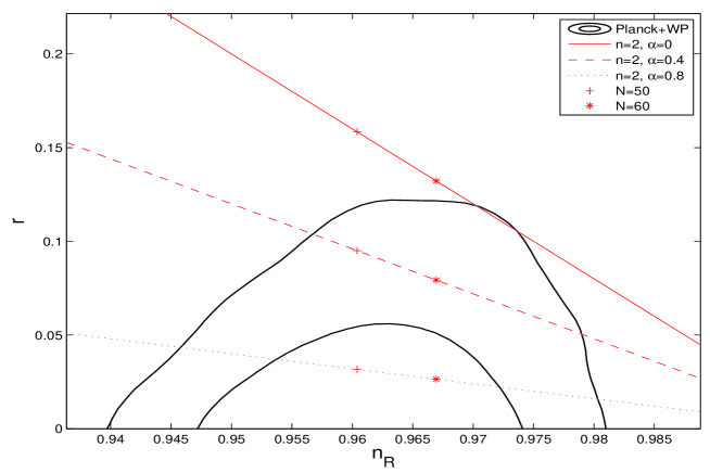
Figure 1: Marginalized joint 68% and 95% CL regions for $n_{\cal R}$ and $r$ without the consistency relation from the Planck+WP data, compared to the theoretical predictions of the model (22) with $n=2$.

We now consider another model with a monomial potential and an inverse monomial GB coupling

$$V(\phi)=V_{0}\phi^{n},\quad\xi(\phi)=\xi_{0}\phi^{-n}.$$ (22)

This class of potentials has been widely studied as the simplest inflationary model. Without the GB coupling the $\phi^{4}$ potential is well outside of the joint $99.7\%$ CL region and the $\phi^{2}$ potential lies outside the joint $95\%$ CL for the Planck+WP+high-$l$ data, as discussed in ade13 . Here we show that the GB coupling may revive this class of potentials. Such a specific choice of GB coupling allows us to find an analytic relation between $r$ and $n_{\cal R}$ in terms of $N$. This model, in which $\epsilon_{1}=n/(4N+n)$, $\delta_{1}=2n\alpha/(4N+n)$ and $\epsilon_{2}=\delta_{2}=4/(4N+n)$, predicts guo10

$$n_{\cal R}-1 = -\frac{2(n+2)}{4N+n},$$ (23)

$$r = \frac{16n(1-\alpha)}{4N+n}.$$ (24)

To confront the theoretical predictions with the Planck constraints, in figure 1 we plot the values of $n_{\cal R}$ and $r$ in the model with $n=2$ for different values of $N$ and $\alpha$. We see that for a fixed number of e-folds the parameter $\alpha$ can shift the predicted $r$ vertically and keep $n_{\cal R}$ invariant. Figure 1 shows that the model with a positive $\alpha$ can be consistent with the Planck data while one with a negative $\alpha$ is disfavored.

III.3 chaotic inflation with a dilaton-like coupling

In the two classes of models discussed above, we notice that the GB coupling and potential satisfy $\xi(\phi)V(\phi)=3\alpha/4$, so that the relation between $r$ and $n_{\cal R}$ can analytically be expressed in terms of model parameters. Here we consider a more general model with a monomial potential and a dilaton-like coupling

$$V(\phi)=V_{0}\phi^{n}\;,\quad\xi(\phi)=\xi_{0}e^{-\lambda\phi}.$$ (25)

For this model the Hubble and GB flow parameters are given by

$$\epsilon_{1} =\frac{n\left(n-\alpha\lambda e^{-\lambda\phi}\phi^{n+1}\right)}{2\phi^{2}}\;,$$ (26)

$$\epsilon_{2} =\frac{2n-\alpha\lambda e^{-\lambda\phi}\phi^{n+1}(\lambda\phi-n+1)}{\phi^{2}}\;,$$ (27)

$$\delta_{1} =\frac{\alpha\lambda e^{-\lambda\phi}\phi^{n+1}\left(n-\alpha\lambda e^{-\lambda\phi}\phi^{n+1}\right)}{\phi^{2}}\;,$$ (28)

$$\delta_{2} =\frac{n(\lambda\phi-n+1)-2\alpha\lambda e^{-\lambda\phi}\phi^{n+1}(\lambda\phi-n)}{\phi^{2}}\;.$$ (29)

From Eqs. (13) and (14) one gets the scalar spectral index and tensor-to-scalar ratio

$$n_{\mathcal{R}}-1 =\frac{-n(n+2)+\alpha\lambda e^{-\lambda\phi}\phi^{n+1}(2\lambda\phi-n)}{\phi^{2}}\;,$$ (30)

$$r =\frac{8\left(n-\alpha\lambda e^{-\lambda\phi}\phi^{n+1}\right)^{2}}{\phi^{2}}\;,$$ (31)

which involve three model parameters $n$, $\lambda$ and $\alpha$ in the slow-roll approximation. Hereafter, we restrict ourselves to a quadratic potential, $n=2$, often considered the simplest example for inflation lin83 . The value of $\phi$ in (30) and (31) depends on the number of e-folds and the value of $\phi_{\rm end}$ by setting max($\epsilon_{i},\delta_{i})(\phi_{\rm end})=1$. For simplicity we set $N=60$.

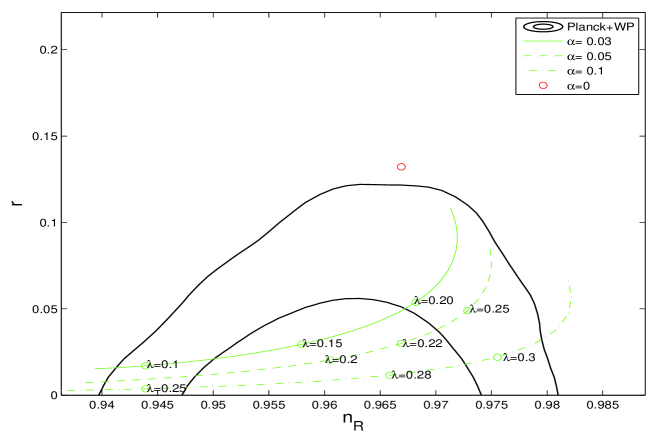
Figure 2: Predicted $n_{\cal R}$ versus $r$ in the model (25) with $n=2$ for different values of $\lambda$ and $\alpha$. Here we choose $N=60$. The contours show the 68% and 95% CL from the Planck+WP data.

In figure 2 we plot the scalar spectral index and tensor-to-scalar ratio for different values of $\lambda$ and $\alpha$. There exist parameter regions in which the predicted $n_{\cal R}$ and $r$ are excellently consistent with the Planck constraints. We see that the scalar spectral index is sensitive to $\lambda$ for a given value of $\alpha$. Compared to the inverse monomial coupling discussed in subsection B, these observable quantities are more sensitive to the dilaton-like coupling.

IV discussions and conclusions

In this general slow-roll inflationary scenario, the potential dominates the energy density of the Universe and the contribution from the GB coupling is ignorable. The GB coupling may slow down the evolution of the inflaton by balancing the potential force, which decreases the energy scale of the potential to be in agreement with the observed amplitude of scalar perturbation. Hence, the tensor-to-scalar ratio is suppressed. In principle, even for a steep potential slow-roll inflation can occur with the help of the non-minimal coupling of the inflaton to the GB term. In the framework of the standard slow-roll inflation, it known that the energy scale of inflation can be established by the detection of the amplitude of tensor perturbations ade13 ; guo11 . In the presence of the GB coupling, one need further measure the tensor tilt to establish the energy scale of inflation because the new degree of freedom is introduced by the GB coupling.

Under the general slow-roll approximation, since the Hubble and GB flow parameters, $\epsilon_{i}$ and $\delta_{i}$, are much smaller than 1, the propagation speed of scalar perturbations (9) is very close to 1. It is shown that the effect of the GB coupling on primordial non-Gaussianities appears indirectly through the change of $c^{2}_{\cal R}$ fel11 . For the equilateral configuration, the non-linearity parameter is fel11

$$f_{\rm NL}^{\rm equil}\sim\frac{55}{36}\epsilon_{1}-\frac{25}{72}\delta_{1}+\frac{5}{12}\frac{2\epsilon_{1}\epsilon_{2}-\delta_{1}\delta_{2}}{2\epsilon_{1}-\delta_{1}},$$ (32)

which means that these extra contributions from the GB coupling remain of the order of small slow-roll parameters, just as in the minimally-coupled single-field case. This is consistent with the Planck’s results ade13n .

In this paper we have applied the general slow-roll formalism to some specific inflationary models in which the inflaton has a direct coupling with the GB term. Since the consistency relation between the tensor-to-scalar ratio and tensor spectral index is broken by the GB coupling, we obtained a slightly tighter constraints on the tensor-to-scalar ratio using the Planck+WP data when the tensor spectral index is allowed to vary freely. In the $r-n_{\cal R}$ plane we then confront the models with observational constraints. We found that there exit parameter regions in which the predicted $r$ and $n_{\cal R}$ are excellently consistent with the Planck constraints. Moreover, in the scenario the non-linearity parameter is of the order of slow-roll parameters, which is in agreement with the observational constraints.

- (1) G. Hinshaw et al. [WMAP Collaboration], arXiv:1212.5226.
- (2) P. A. R. Ade et al. [Planck Collaboration], arXiv:1303.5082.
- (3) C. G. Callan, Jr., E. J. Martinec, M. J. Perry and D. Friedan, Nucl. Phys. B 262, 593 (1985); D. J. Gross and J. H. Sloan, Nucl. Phys. B 291, 41 (1987).
- (4) I. Antoniadis, E. Gava and K. S. Narain, Nucl. Phys. B 383, 93 (1992) [arXiv:hep-th/9204030]; I. Antoniadis, J. Rizos and K. Tamvakis, Nucl. Phys. B 415, 497 (1994) [arXiv:hep-th/9305025].
- (5) S. Kawai, M. -a. Sakagami and J. Soda, Phys. Lett. B 437, 284 (1998) [arXiv:gr-qc/9802033]; S. Kawai and J. Soda, Phys. Lett. B 460, 41 (1999) [arXiv:gr-qc/9903017].
- (6) S. Tsujikawa, Phys. Lett. B 526, 179 (2002) [arXiv:gr-qc/0110124]; A. Toporensky and S. Tsujikawa, Phys. Rev. D 65, 123509 (2002) [arXiv:gr-qc/0202067]; S. Tsujikawa, R. Brandenberger and F. Finelli, Phys. Rev. D 66, 083513 (2002) [arXiv:hep-th/0207228].
- (7) K. Bamba, Z. K. Guo and N. Ohta, Prog. Theor. Phys. 118, 879 (2007) [arXiv:0707.4334]; K. Andrew, B. Bolen and C. A. Middleton, Gen. Rel. Grav. 39, 2061 (2007) [arXiv:0708.0373]; R. Chingangbam, M. Sami, P. V. Tretyakov and A. V. Toporensky, Phys. Lett. B 661, 162 (2008) [arXiv:0711.2122]; I. V. Kirnos and A. N. Makarenko, arXiv:0903.0083.
- (8) S. Nojiri, S. D. Odintsov and M. Sasaki, Phys. Rev. D 71, 123509 (2005) [arXiv:hep-th/0504052]; G. Cognola, E. Elizalde, S. Nojiri, S. D. Odintsov and S. Zerbini, Phys. Rev. D 73, 084007 (2006) [arXiv:hep-th/0601008]; T. Koivisto and D. F. Mota, Phys. Lett. B 644, 104 (2007) [astro-ph/0606078]; S. Tsujikawa and M. Sami, JCAP 0701, 006 (2007) [arXiv:hep-th/0608178]; T. Koivisto and D. F. Mota, Phys. Rev. D 75, 023518 (2007) [hep-th/0609155]; B. M. Leith and I. P. Neupane, JCAP 0705, 019 (2007) [arXiv:hep-th/0702002]; B. C. Paul and S. Ghose, Gen. Rel. Grav. 42, 795 (2010) [arXiv:0809.4131]; M. R. Setare and E. N. Saridakis, Phys. Lett. B 670, 1 (2008) [arXiv:0810.3296]; J. Sadeghi, M. R. Setare and A. Banijamali, Phys. Lett. B 679, 302 (2009) [arXiv:0905.1468]; J. Sadeghi, M. R. Setare and A. Banijamali, Eur. Phys. J. C 64, 433 (2009) [arXiv:0906.0713]; P. Wu and H. Yu, Mod. Phys. Lett. A 25, 2325 (2010); J. Moldenhauer, M. Ishak, J. Thompson and D. A. Easson, Phys. Rev. D 81, 063514 (2010) [arXiv:1004.2459]; S. Nojiri and S. D. Odintsov, Phys. Rept. 505, 59 (2011) [arXiv:1011.0544]; M. Iihoshi, Gen. Rel. Grav. 43, 1571 (2011) [arXiv:1011.2088]; K. Maeda, N. Ohta and R. Wakebe, Eur. Phys. J. C 72, 1949 (2012) [arXiv:1111.3251].
- (9) R. A. Brown, R. Maartens, E. Papantonopoulos and V. Zamarias, JCAP 0511, 008 (2005) [arXiv:gr-qc/0508116]; J. H. He, B. Wang and E. Papantonopoulos, Phys. Lett. B 654, 133 (2007) [arXiv:0707.1180]; E. N. Saridakis, Phys. Lett. B 661, 335 (2008) [arXiv:0712.3806].
- (10) J. -c. Hwang and H. Noh, Phys. Rev. D 61, 043511 (2000) [arXiv:astro-ph/9909480]; C. Cartier, J. -c. Hwang and E. J. Copeland, Phys. Rev. D 64, 103504 (2001) [arXiv:astro-ph/0106197]; J. -c. Hwang and H. Noh, Phys. Rev. D 71, 063536 (2005) [arXiv:gr-qc/0412126].
- (11) M. Satoh, S. Kanno and J. Soda, Phys. Rev. D 77, 023526 (2008) [arXiv:0706.3585]; M. Satoh and J. Soda, JCAP 0809, 019 (2008) [arXiv:0806.4594]; M. Satoh, JCAP 1011, 024 (2010) [arXiv:1008.2724]; K. Nozari and N. Rashidi, arXiv:1310.3989.
- (12) Z. K. Guo, N. Ohta and S. Tsujikawa, Phys. Rev. D 75, 023520 (2007) [arXiv:hep-th/0610336].
- (13) Z. K. Guo and D. J. Schwarz, Phys. Rev. D 80, 063523 (2009) [arXiv:0907.0427].
- (14) Z. K. Guo and D. J. Schwarz, Phys. Rev. D 81, 123520 (2010) [arXiv:1001.1897].
- (15) D. J. Schwarz, C. A. Terrero-Escalante and A. A. Carcia, Phys. Lett. B 517, 243 (2001) [arXiv:astro-ph/0106020]; S. M. Leach, A. R. Liddle, J. Martin and D. J. Schwarz, Phys. Rev. D 66, 023515 (2002) [arXiv:astro-ph/0202094]; D. J. Schwarz and C. A. Terrero-Escalante, JCAP 0408, 003 (2004) [arXiv:hep-ph/0403129].
- (16) C. Cheng, Q. G. Huang, X. D. Li and Y. Z. Ma, Phys. Rev. D 86, 123512 (2012) [arXiv:1207.6113].
- (17) A. D. Linde, Phys. Lett. B 129, 177 (1983).
- (18) A. R. Liddle, Phys. Rev. D 49, 739 (1994) [astro-ph/9307020]; Z. K. Guo, D. J. Schwarz and Y. Z. Zhang, Phys. Rev. D 83, 083522 (2011) [arXiv:1008.5258]; J. Martin, C. Ringeval and V. Vennin, arXiv:1303.3787; S. Choudhury and A. Mazumdar, arXiv:1306.4496.
- (19) A. De Felice and S. Tsujikawa, JCAP 1104, 029 (2011) [arXiv:1103.1172].
- (20) P. A. R. Ade et al. [Planck Collaboration], arXiv:1303.5084.