On cross-section computation in the brane-world models

Abstract

We present Mathematica7 numerical simulation of the process $pp\!\rightarrow\!\mbox{jet}\!+\!E_{T}^{miss}$ in the framework of modified Randall-Sundrum brane-world model with one infinite and $n$ compact extra dimensions. We compare the energy missing signature with the standard model background $pp\rightarrow\mbox{jet}+\nu\bar{\nu}$, which was simulated at CompHep. We show that the models with numbers of compact extra dimensions greater than 4 can be probed at the protons center-of-mass energy equal 14 TeV. We also find that testing the brane-world models at 7 TeV on the LHC appears to hopeless.

1 Introduction

There are a lot of softwares for simulating a ”New physics” processes at the accelerating experiments. Such programs as CompHep [1] and PYTHIA [2] are among them. Nevertheless, one can consider an infinite extra spatial dimension in the brane-world models. CompHep and PYTHIA are not adopted for such class of models. In this paper we present the numerical simulations of the processes $pp\rightarrow\mbox{jet}+E_{T}^{miss}$ on Mathematica7 in the backgound of modified Randall-Sundrum brane model with one infinite and $n$ compact extra dimensions (RSII-$n$ model). In this brane world model neutral particle such as Z boson and photon can leave our brane, escaping in to the extra dimension of infinite size. In our sumulation we use Gluck Reya Vogt leading order parton distribution functions. In Sec. 2 we compare LO Gluck Reya Vogt PDF [3], by with CTEQ [4], MRST [5] and Alekhin’s [6] LO PDFs. This PDFs coincide at large QCD scale parameter squared $Q^{2}$. In Sec. 3 we compare CompHep and Mathematica7 numerical simulations of the process $pp\rightarrow\mbox{jet}+Z^{0}$ in the framework of standard model. We discuss RSII-$n$ set up in Sec. 4. In Sec. 5 we present numerical simulations of the process $pp\rightarrow\mbox{jet}+E_{T}^{miss}$ in the framework of RSII-$n$ model.

2 Comparison of PDFs at large $Q^{2}$.

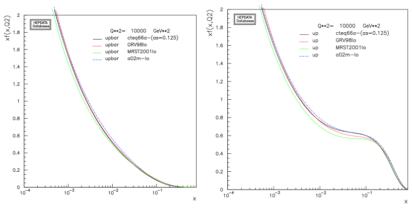
Figure 1: LO PDFs $xu(x,Q^{2})$ and $x\bar{u}(x,Q^{2})$ for GRV, CTEQ, MRST and Alekhin’s collaborations.

In this section we compare LO Gluck Reya Vogt parton distribution functions with CTEQ, MRST and Alekhin’s PDFs. Corresponding distributions for $u$ and $\bar{u}$ quarks are presented on Fig. 1. We suppose that QCD scale parameter is fixed at $Q=100$ GeV. These data are taken from an open High energy physics database [7]. We can see from Fig. 1 that GRV LO PDFs coincide with CTEQ LO, MRST LO and Alekhin’s LO PDFs at large $Q^{2}$. One can obtain an analogous distribution for $d$, $\bar{d}$ quarks and gluon. This means that in the numerical analysis we can use GRV LO PDFs as well as CTEQ, MRST and Alekhins PDFs if $Q^{2}$ is fixed at large values.

3 CompHep vs Mathematica7 in the SM framework.

In this section we compare CompHep and Mathematica7 numerical simulations for the parton cross-sections in the framework of standard model. In Fig. 2 we show the differential cross-section of the processes $dg\rightarrow Z^{0}d$ and $ug\rightarrow Z^{0}u$ versus transverse momentum of $Z^{0}$ boson. The QCD scale is fixed at $Q=1000$ GeV. The diagrams for GRV and CTEQ LO PDFs are coincided. But there is a small discreapancy in $xu(x,Q^{2})$ distribution at high $p_{T}$ values. The analogous distribution can be obtained for the other SM processes such as $\bar{d}g\rightarrow Z^{0}\bar{d}$, $\bar{u}g\rightarrow Z^{0}\bar{u}$, $\bar{d}d\rightarrow Z^{0}g$ and $\bar{u}d\rightarrow Z^{0}g$. Nevertheless, the main contribution to the process $pp\rightarrow\mbox{jet}+Z^{0}$ comes from the gluon cross-sections which are shown on Fig. 2.

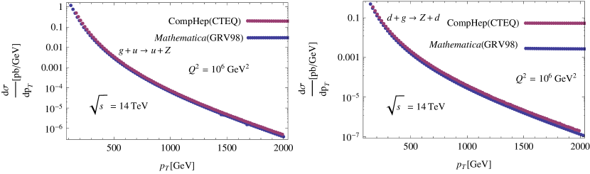
Figure 2: Comparison of differential distribution for the processes $dg\rightarrow Z^{0}d$ and $ug\rightarrow Z^{0}u$ simualated at CompHep and Mathematica7 in the framework of standard model.

4 Modified Randall-Sundrum model

In this section we discuss a peculiar features of the modified RSII-$n$ model. Let us consider a 3-brane with $n$ compact dimensions embeeded in a $(5+n)$ space-time AdS metric

$$ds^{2}=a(z)^{2}(\eta_{\mu\nu}dx^{\mu}dx^{\nu}-\delta_{ij}d\theta^{i}d\theta^{j})-dz^{2}.$$ (1)

This metric was suggested by T. Gherghetta and M. Shaposhnikov [8]. Here $z$ is the infinite extra dimension, $\theta_{i}$ are the compact extra-dimensions $\theta_{i}\in[0,2\pi R_{i}]$, $i=\overline{1,n}$, $R_{i}$ are the sizes of compact extra dimensions, $n$ - is the number of compact extra dimensions, $a(z)=e^{-k|z|}$ is a warp factor from Randall-Sundrum model and $k$ is a AdS curvature.

We put entire $SU(2)\times U(1)$ gauge sector, as well as the Higgs sector into the bulk space, but the fermions of the standard modell are supposed to be localized on the brane. The action of the model is

$$S=\int d^{4}x\,dz\prod^{n}_{i=1}\frac{d\theta_{i}}{2\pi R_{i}}\sqrt{g}\Bigl{[}-\frac{1}{2}|\,W_{MN}\,|^{2}+m^{2}_{W}|\,W_{M}\,|^{2}-\frac{1}{4}Z^{2}_{MN}+\frac{1}{2}m^{2}_{Z}Z^{2}_{M}$$

$$-\frac{1}{4}F^{2}_{MN}+\frac{1}{2}(\partial_{M}\chi)^{2}-\frac{1}{2}m^{2}_{\chi}\chi^{2}+\delta(z)\mathcal{L}_{ferm}\Bigr{]},$$ (2)

where $m_{W}^{2}=\frac{1}{4}\widetilde{g}_{2}^{2}v^{2}$, $m_{Z}^{2}=\frac{1}{4}(\widetilde{g}_{2}^{2}+\widetilde{g}_{1}^{2})v^{2}$ and $m^{2}_{\chi}=\lambda v^{2}$ are the bulk masses of the gauge fields and Higgs respectively. We also suppose the size of the compact extra dimension to be $1/R_{i}\gg\sqrt{s}$. This means that corresponding KK excitations become infinitely heavy and dissappear from the spectrum.

Table 1: The lower bounds on the AdS curvature $k$ for various  $n$.

$n$	$1$	$2$	$3$	$4$	$5$	$6$
$k,\mbox{GeV}$	$5.5\times 10^{6}$	$20\times 10^{3}$	$2.5\times 10^{3}$	$900$	$400$	$300$

Since the $Z$-boson is not exactly localized on the brane, one can obtain the bounds on number of compact extra dimension $n$ and the AdS curvature $k$. We require that the invisible width decay of $Z$-boson in RSII-n model is bounded by the experimental uncertainty of the total $Z$-boson width decay [9]:

$$\Gamma_{RS}(M_{Z})\leq\Delta\Gamma^{Z}_{tot}=1.5\,\mbox{MeV}.$$

where

$$\Gamma^{Z}_{RS}=\frac{2\pi}{n\Gamma^{2}\left(\frac{n}{2}\right)}M_{Z}\left(\frac{M_{Z}}{2k}\right)^{n},$$ (3)

is the invisible decay rate of $Z^{0}_{bulk}$ boson [10]. These bounds are shown in Tab. 1. We use these values of $k$ when presenting the numerical simulations in Sec. 5

5 Numerical simulation of the process $pp\rightarrow\mbox{jet}+E_{T}^{miss}$.

In this section we discuss numerical simulation of the process $pp\to\mbox{jet}+Z_{bulk}(\gamma_{bulk})$ at the collider experiment in the frame work of RSII-$n$ model. Here the jet originates from gluon or quark, and $Z_{bulk}$ and $\gamma_{bulk}$ are the particles which escape the brane.

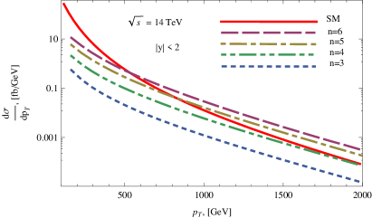
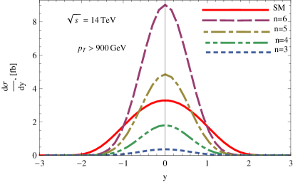
Figure 3: Differential cross section of the process $pp\to\mbox{jet}+Z_{bulk}(\gamma_{bulk})$ for $n=3,4,5,6$ at the center-of-mass energy of protons equal $\sqrt{s}=14$TeV. The standard model background is $pp\to\mbox{jet}+\nu\bar{\nu}$.

The differential cross-section of this process is

$$\frac{d^{2}\sigma}{dy\,p_{T}dp_{T}}\!\!=\!\!\int dx_{1}dx_{2}\!\!\!\sum_{i,j=q,\bar{q},g}\!\!\!\frac{f_{i}(x_{1},Q^{2})}{x_{1}}\frac{f_{j}(x_{2},Q^{2})}{x_{2}}\frac{1}{4\pi s\,m}\,\overline{\sum_{k}}|\mathcal{M}_{ij\to k(bulk)}|^{2}$$ (4)

where $\mathcal{M}_{ij\rightarrow k(bulk)}$ are parton amplitudes for the subprocesses $gq\to qZ_{bulk}(\gamma_{bulk})$, $\bar{q}q\to gZ_{bulk}(\gamma_{bulk})$ (see Ref. [10] for details); $m$ is a bulk invariant mass of $Z_{bulk}$ and $\gamma_{bulk}$:

$$m^{2}=sx_{1}x_{2}-x_{1}p_{T}\sqrt{s}\e^{-y}-x_{2}p_{T}\sqrt{s}\e^{+y},$$

and $f_{i}(x_{1},Q^{2})$ are GRV LO PDFs [3]. The QCD scale parameter is fixed at $Q=1$ TeV. We compare the distribution (4) with the standard model background $pp\to\mbox{jet}+\nu\bar{\nu}$. This background was computed by CompHep program [1].

Let us consider the case of the proton center-of-mass energy equal 14 TeV. In Fig. 3 we show $p_{T}$ and jet rapidity distributions of the process $pp\to\mbox{jet}+Z_{bulk}(\gamma_{bulk})$. One can see from Fig. 3 that if $n=6$ and $n=5$, then the signal dominates over the background for $p_{T}>500$ GeV and $p_{T}>750$ GeV, correspondingly. And the background dominates over the signal for $n=3,4$. Once the larger values of $k$ correspond to the smaller $n$ (see Tab. 1), so that the signal cross section grows with the increase of $n$. It is clear from Fig. 3 that the jet rapidity distributions are correlated with the jet transverse momentum distributions.

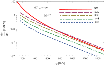
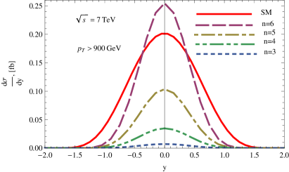
Figure 4: Same as in Fig. 3, but for the energy of protons equal 7 TeV.

In Tab. 2 we show the integrated luminosity and number of signal events needed for $5\sigma$ discovery at the LHC center-of-mass energy equal $14$ TeV. Where the cuts in jet rapidity and transverse momentum are $|y|<2$, $p_{T}>900$ GeV.

Table 2: Integrated luminosity $\mathcal{L}$ and numbers of signal events $N_{S}$ for various $n$, at the LHC center-of-mass energy $\sqrt{s}=$ 14 TeV.

$n$	$3$	$4$	$5$	$6$
$\mathcal{L},\mbox{fb}^{-1}$	$7.1\times 10^{2}$	$3.7\times 10^{1}$	$7.5$	$3.1$
$N_{S}$	$3.6\times 10^{2}$	$10^{2}$	$5\times 10^{1}$	$3.8\times 10^{1}$

Now let us consider the case $\sqrt{s}=7$ TeV. In Fig. 4 we show the jet transverse momentum and rapidity distributions. Only the case with $n\geq 6$ can be probed, since the background dominates over the signal for $n=3,4,5$. The integrated luminosity required for $5\sigma$ discovery at the LHC is $\mathcal{L}=200\,\mbox{fb}^{-1}$ even for $n=6$.

6 Summary

In the framework of RSII-n model the distributions of the process $pp\rightarrow\mbox{jet}+Z^{0}_{bulk}(\gamma_{bulk})$ were simulated on Mathematica7 with GRV LO PDFs implemented. The detection of the extra spatial dimension at 7 TeV appears to be hopeless. At the LHC energy equal 14 TeV the luminosity needed for $5\sigma$ discovery is in the range $(10-100)\mbox{fb}^{-1}$.

7 Acknowledgements

We are indebted to A. B. Arbuzov and A. L. Kataev, for helpful discussions and advices, to ACAT 2013 Organizing Comittee and in particular Bin Gong for support and hospitality. This work was supported in part by grants of Russian Ministry of Education and Science NS-5590.2012.2 and GK-8412, grants of the President of Russian Federation MK-2757.2012.2, and grants of RFBR 12-02-31595 MOL A and RFBR 13-02-01127 A.

References

References

- [1] Boos E Bunichev E Dubinin M Dudko L Edneral V Ilyin V Kryukov A and Savrin V 2008 PoS ACAT 08 008
- [2] Sjostrand T Eden P Friberg C Lonnblad L Miu G Mrenna S and Norrbin E 2001 Comput. Phys. Commun. 135 238
- [3] Gluck M Reya E and Vogt A 1998 Eur. Phys. J. C 5 461
- [4] Pumplin J Stump D Huston J Lai H Nadolsky P and Tung W 2002 JHEP 0207 012
- [5] Martin A Roberts R Stirling W and Thorne R 2002 Phys. Lett. B 531 216
- [6] Alekhin S 2003 Phys. Rev. D 68 014002
- [7] http://hepdata.cedar.ac.uk/pdf/pdf3.html
- [8] Gherghetta T and Shaposhnikov M 2000 Phys. Rev. Lett. 85 240
- [9] Amsler C et al. 2008 Phys. Lett. 667 1
- [10] Kirpichnikov D 2012 Phys. Rev. D 85 115008