Critical points of multidimensional random Fourier series: variance estimates

Abstract.

We investigate the number of critical points of a Gaussian random smooth function $u^{\varepsilon}$ on the $m$-torus $T^{m}:=\mathbb{R}^{m}/\mathbb{Z}^{m}$. The randomness is specified by a fixed nonnegative Schwartz function $w$ on the real axis and a small parameter $\varepsilon$ so that, as $\varepsilon\to 0$, the random function $u^{\varepsilon}$ becomes highly oscillatory and converges in a special fashion to the Gaussian white noise. Let $N^{\varepsilon}$ denote the number of critical points of $u^{\varepsilon}$. We describe explicitly in terms of $w$ two constants $C,C^{\prime}$ such that as $\varepsilon$ goes to the zero, the expectation of the random variable ${\varepsilon}^{-m}N^{\varepsilon}$ converges to $C$, while its variance is extremely small and behaves like $C^{\prime}{\varepsilon}^{m}$.

1. Introduction

1.1. The setup

Consider the $m$-dimensional torus ${\mathbb{T}}^{m}:={\mathbb{R}}^{m}/{\mathbb{Z}}^{m}$ with angular coordinates $\theta_{1},\dotsc,\theta_{m}\in{\mathbb{R}}/{\mathbb{Z}}$ equipped with the flat metric

$$g:=\sum_{j=1}^{m}(d\theta_{j})^{2},\;\;{\rm vol}_{g}({\mathbb{T}}^{m})=1.$$

The eigenvalues of the corresponding Laplacian $\Delta=-\sum_{k=1}^{m}\partial^{2}_{\theta_{k}}$ are

$$(2\pi)^{2}|\vec{k}|^{2},\;\;\vec{k}=(k_{1},\dotsc,k_{m})\in{\mathbb{Z}}^{m}.$$

For $\vec{\theta}=(\theta_{1},\dotsc,\theta_{m})\in{\mathbb{R}}^{m}$ and $\vec{k}\in{\mathbb{Z}}^{m}$ we set

$$\langle\vec{k},\vec{\theta}\rangle=\sum_{j}k_{j}\theta_{j}.$$

Denote by $\prec$ the lexicographic order on ${\mathbb{R}}^{m}$. An orthonormal basis of $L^{2}({\mathbb{T}}^{m})$ is given by the functions $(\Psi_{\vec{k}})_{\vec{k}\in{\mathbb{Z}}^{m}}$, where

$$\Psi_{\vec{k}}(\vec{\theta})=\begin{cases}1,&\vec{k}=0\\ \sqrt{2}\sin 2\pi\langle\vec{k},\vec{\theta}\rangle,&\vec{k}\succ\vec{0},\\ \sqrt{2}\cos 2\pi\langle\vec{k},\vec{\theta}\rangle,&\vec{k}\prec\vec{0}.\end{cases}$$

Fix a nonnegative, even Schwartz function $w\in\mathcal{S}({\mathbb{R}})$, set $w_{\varepsilon}(t)=w({\varepsilon}t)$. In particular, there exists a unique Schwartz function ${\varphi}\in\mathcal{S}({\mathbb{R}})$ such that

$$w(t)={\varphi}(t^{2}),\;\;\forall t\in{\mathbb{R}}.$$ (1.1)

Consider the random function

$${\mathbf{u}}^{\varepsilon}(\vec{\theta})=\sum_{\vec{k}\in{\mathbb{Z}}^{m}}X^{\varepsilon}_{\vec{k}}\Psi_{\vec{k}}(\vec{\theta}),$$ (1.2)

where the coefficients $X^{\varepsilon}_{\vec{k}}$ are independent Gaussian random variables with mean $0$ and variances

$$\operatorname{\boldsymbol{var}}(X_{\vec{k}})=w_{\varepsilon}(2\pi|\vec{k}|)=w(2\pi{\varepsilon}|\vec{k}|).$$

For ${\varepsilon}>0$ sufficiently small the random function ${\mathbf{u}}^{\varepsilon}$ is almost surely (a.s.) smooth and Morse. By energy landscape of ${\mathbf{u}}^{\varepsilon}$ we understand the catalogue containing the basic information about the critical points of ${\mathbf{u}}^{\varepsilon}$: their location, their indices, and their corresponding critical values. A first information about the energy landscape concerns the number of the critical points. Let $N({\mathbf{u}}^{\varepsilon})$ denote the number of critical points of ${\mathbf{u}}^{\varepsilon}$. We denote by $N_{\varepsilon}$ the expectation the random variable $N({\mathbf{u}}^{\varepsilon})$,

$$N_{\varepsilon}:=\boldsymbol{E}\Bigl{(}\;N({\mathbf{u}}^{\varepsilon})\;\Bigr{)},$$

and by $\operatorname{\boldsymbol{var}}_{\varepsilon}$ its variance

$$\operatorname{\boldsymbol{var}}^{\varepsilon}=\boldsymbol{E}\Bigl{(}\,\bigl{(}\,N({\mathbf{u}}^{\varepsilon})-N_{\varepsilon}\,\bigr{)}^{2}\,\Bigr{)}=\boldsymbol{E}\bigl{(}\,N({\mathbf{u}}^{\varepsilon})^{2}\,\bigr{)}-N_{\varepsilon}^{2}.$$

We are interested in the the small ${\varepsilon}$ behavior of the random variable $N_{\varepsilon}$.

To understand the analytic significance of the ${\varepsilon}\to 0$ limit it is best to think of the special case when $w$ “approximates” the characteristic function of the interval $[-1,1]$, i.e., it is supported in $[-1,1]$ and it is identically $1$ in a neighborhood of $0$. For fixed ${\varepsilon}$, ${\mathbf{u}}^{\varepsilon}$ is a trigonometric polynomial: the terms corresponding to $|\vec{k}|>{\varepsilon}$ do not contribute to ${\mathbf{u}}^{\varepsilon}$. If we formally let ${\varepsilon}\searrow 0$ in (1.2) , then we deduce that ${\mathbf{u}}^{\varepsilon}$ converges to the random Fourier series

$$\sum_{\vec{k}\in{\mathbb{Z}}^{m}}X^{0}_{\vec{k}}\Psi_{\vec{k}}(\vec{\theta}),$$

where the coefficients $X^{0}_{\vec{k}}$ are independent, standard normal random variables with mean $0$ and variance $1$.

The above series is not convergent to any function in any meaningful way but, as explained in [5], it converges almost surely in the sense of distributions to a random distribution on the torus, the Gaussian white noise. For ${\varepsilon}>0$ very small, the trigonometric polynomial ${\mathbf{u}}^{\varepsilon}$ is highly oscillatory and we expect it to have many critical points, i.e., $N_{\varepsilon}\to\infty$ as ${\varepsilon}\searrow 0$ . In [11] proved a more precise statement, namely

$$N_{\varepsilon}\sim C_{m}(w){\varepsilon}^{-m}\bigl{(}1+O({\varepsilon})\,\bigr{)}\;\;\mbox{as ${\varepsilon}\searrow 0$},$$ (1.3)

where $C_{m}(w)$ is a certain explicit constant positive constant that depends only on $m$ and $w$. In this paper we describe the small ${\varepsilon}$ asymptotics for the variance of the normalized random variable $\frac{1}{N_{\varepsilon}}N({\mathbf{u}}^{\varepsilon})$. In particular, we prove that this random variable is highly concentrated around its mean.

1.2. The main result

The goal of this paper is an asymptotic formula (as ${\varepsilon}\searrow 0$) for the variance of the random variable $N(\,{\mathbf{u}}^{\varepsilon}\,)$.

Theorem 1.1.

There exists a constant $C^{\prime}_{m}(w)\geq 0$ such that

$$\operatorname{\boldsymbol{var}}^{\varepsilon}\sim C^{\prime}_{m}(w){\varepsilon}^{-m}\bigl{(}\,1+O({\varepsilon}^{N})\,\bigr{)},\;\;\forall N>0,\;\;\mbox{as ${\varepsilon}\searrow 0$}.$$ (1.4)

Consider the normalized random variables

$$\widehat{N}({\mathbf{u}}^{\varepsilon}):=\frac{1}{N_{\varepsilon}}N({\mathbf{u}}^{\varepsilon})=\frac{1}{\boldsymbol{E}(\,N({\mathbf{u}}^{\varepsilon})\,)}N({\mathbf{u}}^{\varepsilon}).$$

Corollary 1.2.

If $({\varepsilon}_{k})$ is a sequence of positive numbers such that $\sum_{k}{\varepsilon}_{k}^{m}<\infty$, then sequence of random variables $\widehat{N}_{{\varepsilon}_{k}}$ converges almost surely to $1$.

Proof.

The equalities (1.3) and (1.4) imply that the variance $\widehat{\operatorname{\boldsymbol{var}}}^{\varepsilon}$ of $\widehat{N}({\mathbf{u}}^{\varepsilon})$ is extremely small,

$$\widehat{\operatorname{\boldsymbol{var}}}^{\varepsilon}\sim\frac{C^{\prime}_{m}(w)}{C_{m}(w)^{2}}{\varepsilon}^{m}\;\;\mbox{as ${\varepsilon}\searrow 0$}.$$ (1.5)

Now conclude using Chebysev’s inequality and the Borel-Cantelli’s lemma. $\hbox to0.0pt{$\sqcap$\hss}\sqcup$

The constant $C_{m}^{\prime}(w)$ has an explicit, albeit very complicated description. Here is the gist of it.

Denote by $\operatorname{\mathbf{Sym}}_{m}$ the space of real symmetric $m\times m$ matrices. The group $O(m)$ acts on $\operatorname{\mathbf{Sym}}_{m}$ by conjugation and we denote by $\mathcal{G}_{m}$ the space of $O(m)$-invariant Gaussian measures on $\operatorname{\mathbf{Sym}}_{m}$. This is a $2$-dimensional convex cone described explicitly in Appendix C. Then

$$C_{m}(w)=\frac{1}{(2\pi d_{m})^{\frac{m}{2}}}\left(\int_{\operatorname{\mathbf{Sym}}_{m}}|\det A|\,\boldsymbol{\Gamma}_{h_{m},h_{m}}(dA)\right),$$

where $h_{m},d_{m}$ are certain momenta of $w$ defined in (2.6) and the Gaussian measure $\boldsymbol{\Gamma}_{h_{m},h_{m}}\in\mathcal{G}_{m}$ is described in (C.4).

For any $\eta\in{\mathbb{R}}^{m}\setminus 0$ we denote by $O_{\eta}(m)$ the subgroup of $O(m)$ consisting of orthogonal maps which fix $\eta$. We denote by $\mathcal{G}_{m,\eta}$ the space of $O_{\eta}(m)$-invariant Gaussian measures on $\operatorname{\mathbf{Sym}}_{m}$. This is a $5$-dimensional convex cone described explicitly in Appendix C. We set $\operatorname{\mathbf{Sym}}_{m}^{\times 2}=\operatorname{\mathbf{Sym}}_{m}\oplus\operatorname{\mathbf{Sym}}_{m}$ so that the elements in $B=\operatorname{\mathbf{Sym}}_{m}^{\times 2}$ have the form $B=B^{-}\oplus B^{+}$, $B^{\pm}\in\operatorname{\mathbf{Sym}}_{m}$.

The constant $C^{\prime}_{m}(w)$ is expressed in terms of a family of Gaussian random matrices

$$B_{\eta}=B_{\eta}^{-}\oplus B_{\eta}^{+}\in\operatorname{\mathbf{Sym}}_{m}^{\times 2},\;\;\eta\in{\mathbb{R}}^{m}\setminus 0.$$

We denote by $\bar{\boldsymbol{\Xi}}^{0}(\eta)$ the distribution of $B_{\eta}$. The Gaussian measure $\bar{\boldsymbol{\Xi}}^{0}(\eta)$ has an explicit but quite complicated description detailed in Appendix B.

The correspondence $\eta\mapsto\bar{\boldsymbol{\Xi}}^{0}(\eta)$ is equivariant with respect to the action of $O(m)$ on ${\mathbb{R}}^{m}$ and its diagonal action on the space of Gaussian measures on $\operatorname{\mathbf{Sym}}_{m}^{\times 2}$. The components $B_{\eta}^{\pm}$ are identically distributed, and their distributions are certain explicit Gaussian measures in $\mathcal{G}_{m,\eta}$. These components are not independent, but become less and less correlated as $|\eta|\to\infty$. In fact, as $|\eta|\to\infty$ the Gaussian measure $\bar{\boldsymbol{\Xi}}^{0}(\eta)$ converges to the product of the Gaussian measures $\boldsymbol{\Gamma}_{\infty}=\boldsymbol{\Gamma}_{h_{m},h_{m}}\times\boldsymbol{\Gamma}_{h_{m},h_{m}}$. We denote by $\boldsymbol{E}_{\bar{\boldsymbol{\Xi}}^{0}(\eta)}(|\det B|)$ the expectation of the random variable $|\det B_{\eta}|$.

To each $\eta\in{\mathbb{R}}^{M}\setminus 0$ we associate the symmetric $2m\times 2m$ matrix

$$\mathcal{H}(V,\eta)=\left[\begin{array}[]{cc}-\operatorname{Hess}(V,0)&-\operatorname{Hess}(V,\eta)\\ -\operatorname{Hess}(V,\eta)&-\operatorname{Hess}(V,0)\end{array}\right]$$ (1.6)

where $\operatorname{Hess}(V,\eta)$ denotes the Hessian at $\eta$ of the function $V:{\mathbb{R}}^{n}\to{\mathbb{R}}$,

$$V(\xi)=\int_{{\mathbb{R}}^{m}}e^{-\boldsymbol{i}(\xi,x)}w(|x|)|dx|.$$

We set

$$K(\eta):=\frac{1}{\sqrt{\det 2\pi\mathcal{H}(V,\eta)}}.$$

Then

$$K(\eta)\sim const.|\eta|^{-m}\;\;\mbox{as $\eta\to 0$},$$

and as $\eta\to\infty$ the quantity $K(\eta)$ approaches rapidly the constant

$$K(\infty)=\frac{1}{\det\bigl{(}\,2\pi\operatorname{Hess}(V,0)\,\bigr{)}}.$$

Then

$$C_{m}^{\prime}(w)=C_{m}(w)+\int_{{\mathbb{R}}^{m}}\Bigr{(}\,K(\eta)\boldsymbol{E}_{\bar{\boldsymbol{\Xi}}^{0}(\eta)}\bigl{(}\,|\det B|\,\bigr{)}-K(\infty)\boldsymbol{E}_{\boldsymbol{\Gamma}_{\infty}}\bigl{(}\,|\det B|\,\bigr{)}\,\Bigr{)}|d\eta|.$$

Let us point out that

$$C_{m}(w)^{2}=K(\infty)\boldsymbol{E}_{\boldsymbol{\Gamma}_{\infty}}\bigl{(}\,|\det B|\,\bigr{)}.$$

The one-dimensional investigations in [4, 9] suggest that $C_{m}^{\prime}(w)>0$, but all our attempts to proving this were fruitless so far.

1.3. Outline of the proof of Theorem 1.4.

To help the reader better navigate the many technicalities involved in proving (1.4) we describe in this section the bare-bones strategy used in the proof of Theorem 1.4.

Denote by $\boldsymbol{D}$ the diagonal of ${\mathbb{T}}^{m}\times{\mathbb{T}}^{m}$

$$\boldsymbol{D}=\bigl{\{}\,\Theta=(\vec{\theta},\vec{{\varphi}})\in{\mathbb{T}}^{m}\times{\mathbb{T}}^{m};\;\;\vec{\theta}=\vec{{\varphi}}\,\bigr{\}}.$$

We denote by $\mathcal{N}_{\boldsymbol{D}}$ the normal bundle of the embedding $\boldsymbol{D}\hookrightarrow{\mathbb{T}}^{m}\times{\mathbb{T}}^{m}$. For each $r>0$ sufficiently small we denote by $\mathcal{T}_{r}(\boldsymbol{D})$ the tube of radius $r$ around $\boldsymbol{D}$,

$$\mathcal{T}_{r}(\boldsymbol{D})=\Bigl{\{}\Theta\in{\mathbb{T}}^{m}\times{\mathbb{T}}^{m};\;\;\operatorname{dist}\bigl{(}\,\Theta,\boldsymbol{D}\,\bigr{)}<r\,\Bigr{\}},$$

where $\operatorname{dist}$ denotes the geodesic distance on ${\mathbb{T}}^{m}\times{\mathbb{T}}^{m}$ equipped with the product metric $g\times g$.

Denote by $B_{r}(\boldsymbol{D})\subset\mathcal{N}_{\boldsymbol{D}}$ the radius $r$-disk bundle. For $\hbar>0$ sufficiently small, the exponential map induces a diffeomorphism

$$\exp:B_{\hbar}(\boldsymbol{D})\to\mathcal{T}_{\hbar}(\boldsymbol{D}).$$

Fix such a $\hbar$. For $t>0$ we denote by $\mathcal{R}_{t}:\mathcal{N}_{\boldsymbol{D}}\to\mathcal{N}_{\boldsymbol{D}}$ the rescaling by a factor of $t$ along the fibers of the normal bundle $\mathcal{N}_{\boldsymbol{D}}$. Thus, $\mathcal{R}_{t}$ acts as multiplication by $t$ on each fiber of $\mathcal{N}_{\boldsymbol{D}}$.

We can now explain the strategy.

Step 1. Using the Kac-Rice formula we produce a density $\rho_{1}^{\varepsilon}(\vec{\theta})|d\vec{\theta}|$ on ${\mathbb{T}}^{m}$ such that

$$N_{\varepsilon}=\int_{{\mathbb{T}}^{m}}\rho_{1}^{\varepsilon}(\vec{\theta})|d\vec{\theta}|.$$ (1.7)

Set

$$\tilde{\rho}_{1}^{\varepsilon}\bigl{(}\,\Theta\,\bigr{)}:=\rho_{1}^{\varepsilon}(\vec{\theta})\rho_{1}^{\varepsilon}(\vec{{\varphi}}).$$

Step 2. Using the Kac-Rice formula we produce a density $\rho_{2}^{\varepsilon}(\Theta)|d\Theta|$ on ${\mathbb{T}}^{m}\times{\mathbb{T}}^{m}\setminus\boldsymbol{D}$ such that

$$\underbrace{\boldsymbol{E}\bigl{(}\,N({\mathbf{u}}^{\varepsilon})^{2}-N({\mathbf{u}}^{\varepsilon})\,\bigr{)}}_{=:\mu^{\varepsilon}_{(2)}}=\int_{{\mathbb{T}}^{m}\times{\mathbb{T}}^{m}\setminus\boldsymbol{D}}\rho_{2}^{\varepsilon}(\Theta)|d\Theta|.$$ (1.8)

As an aside, let us point out that the ratio

$$\frac{\rho_{2}^{\varepsilon}(\Theta)}{\tilde{\rho}_{1}^{\varepsilon}\bigl{(}\,\Theta\,\bigr{)}}={\varepsilon}^{2m}\frac{\rho_{2}^{\varepsilon}(\Theta)}{C_{m}(w)^{2}}$$

is the so called two-point correlation function of the set of critical points of the random function ${\mathbf{u}}^{\varepsilon}$.

The second combinatorial moment $\mu^{\varepsilon}_{(2)}$ of $N({\mathbf{u}}^{\varepsilon})$ is related to the variance $\operatorname{\boldsymbol{var}}^{\varepsilon}$ via the equality

$$\operatorname{\boldsymbol{var}}^{\varepsilon}=\mu^{\varepsilon}_{(2)}-N_{\varepsilon}^{2}+N_{\varepsilon}.$$ (1.9)

In view of (1.3) the asymptotic estimate (1.4) is equivalent to the existence of a real constant $c$ such that

$$\lim_{{\varepsilon}\searrow 0}{\varepsilon}^{m}\bigl{(}\,\mu_{(2)}^{\varepsilon}-N_{\varepsilon}^{2}\,\bigr{)}=c.$$ (1.10)

Set

$$\delta^{\varepsilon}(\Theta):=\rho_{2}^{\varepsilon}(\Theta)-\tilde{\rho}_{1}^{\varepsilon}(\Theta).$$

Using (1.7) and (1.8) we can rewrite

$$\mu_{(2)}^{\varepsilon}-N_{\varepsilon}^{2}=\underbrace{\int_{\mathcal{T}_{\hbar}(\boldsymbol{D})\setminus\boldsymbol{D}}\delta^{\varepsilon}(\Theta)|d\Theta|}_{=:\boldsymbol{I}_{0}({\varepsilon})}+\underbrace{\int_{{\mathbb{T}}^{m}\times{\mathbb{T}}^{m}\setminus\mathcal{T}_{\hbar}(\boldsymbol{D})}\delta^{\varepsilon}(\Theta)|d\Theta|}_{=:\boldsymbol{I}_{1}({\varepsilon})}.$$ (1.11)

Step 3. Off-diagonal estimates. We show that

$$\lim_{{\varepsilon}\searrow 0}{\varepsilon}^{-N}\boldsymbol{I}_{1}({\varepsilon})=0,\;\;\forall N>0.$$ (1.12)

Step 4. Near-diagonal estimates. Denote by $\beta_{\varepsilon}$ the composition

$$\beta_{\varepsilon}:B_{\hbar/{\varepsilon}}(\boldsymbol{D})\stackrel{{\scriptstyle\mathcal{R}_{\varepsilon}}}{{{\longrightarrow}}}B_{\hbar}(\boldsymbol{D})\stackrel{{\scriptstyle\exp}}{{{\longrightarrow}}}\mathcal{T}_{\hbar}(\boldsymbol{D}).$$

Then

$${\varepsilon}^{m}\boldsymbol{I}_{0}({\varepsilon})=\int_{B_{\hbar/{\varepsilon}}(\boldsymbol{D})\setminus\boldsymbol{D}}\delta^{\varepsilon}\bigl{(}\beta_{\varepsilon}(\eta)\,\bigr{)}|d\eta|,$$

and we will show that the limit

$$\lim_{{\varepsilon}\searrow 0}\int_{B_{\hbar/{\varepsilon}}(\boldsymbol{D})\setminus\boldsymbol{D}}\delta^{\varepsilon}\bigl{(}\beta_{\varepsilon}(\eta)\,\bigr{)}|d\eta|$$ (1.13)

exists and it is finite. It boils down to showing that the function

$$\hat{\delta}^{\varepsilon}:\mathcal{N}_{\boldsymbol{D}}\setminus\boldsymbol{D}\to{\mathbb{R}},\;\;\hat{\delta}^{\varepsilon}(\eta)=\begin{cases}\delta^{\varepsilon}\bigl{(}\beta_{\varepsilon}(\eta)\,\bigr{)},&\eta\in B_{\hbar/{\varepsilon}}(\boldsymbol{D})\setminus\boldsymbol{D}\\ 0,&\mbox{otherwise},\end{cases}$$

converges as ${\varepsilon}\searrow 0$ to an integrable function $\hat{\delta}^{0}:\mathcal{N}_{\boldsymbol{D}}\to{\mathbb{R}}$ and

$$\lim_{{\varepsilon}\searrow 0}\int_{\mathcal{N}_{\boldsymbol{D}}}\hat{\delta}^{\varepsilon}(\eta)|d\eta|=\int_{\mathcal{N}_{\boldsymbol{D}}}\hat{\delta}^{0}(\eta)|d\eta|.$$

This last step is the most challenging part of the proof. A big part of the challenge is the fact that $\hat{\delta}^{\varepsilon}(\eta)$ has a singularity along the zero section of $\mathcal{N}_{\boldsymbol{D}}$.

At this point we think it is useful to provide a few more details to give the reader a better sense of the complexity of the problem. Define a new random function

$${\mathbf{U}}^{\varepsilon}:{\mathbb{T}}^{m}\times{\mathbb{T}}^{m}\to{\mathbb{R}},\;\;{\mathbf{U}}_{\varepsilon}(\vec{\theta},\vec{{\varphi}})={\mathbf{u}}^{\varepsilon}(\vec{\theta})+{\mathbf{u}}^{\varepsilon}(\vec{{\varphi}}).$$

We denote by $N({\mathbf{U}}_{\varepsilon})$ the number of critical points of ${\mathbf{U}}_{\varepsilon}$ situated outside the diagonal. Note that

$$N({\mathbf{U}}^{\varepsilon})=N({\mathbf{u}}^{\varepsilon})^{2}-N({\mathbf{u}}^{\varepsilon})$$

and thus

$$\boldsymbol{E}\bigl{(}\,N({\mathbf{U}}^{\varepsilon})\,\bigr{)}=\mu^{\varepsilon}_{(2)}.$$

The Kac-Rice formula, detailed in Section 2.1, shows that

$$\boldsymbol{E}\bigl{(}\,N({\mathbf{U}}^{\varepsilon})\,\bigr{)}=\int_{{\mathbb{T}}^{m}\times{\mathbb{T}}^{m}\setminus\boldsymbol{D}}\;\underbrace{\frac{1}{\sqrt{\det 2\pi\widetilde{\mathbf{S}}_{\varepsilon}(\Theta)}}\boldsymbol{E}\Bigl{(}\,\bigr{|}\det\operatorname{Hess}{\mathbf{U}}^{\varepsilon}(\Theta)\bigr{|}\,\Bigl{|}\,d{\mathbf{U}}^{\varepsilon}(\Theta)=0\,\Bigr{)}}_{=:\rho_{2}^{\varepsilon}(\Theta)}\,|d\Theta|,$$ (1.14)

where $\widetilde{\mathbf{S}}_{\varepsilon}(\Theta)$ is a symmetric, positive semidefinite $2m\times 2m$ matrix describing the covariance form of the random vector $d{\mathbf{U}}^{\varepsilon}(\Theta)$, and $\boldsymbol{E}(X|Y=0)$ denotes the conditional expectation of the random variable $X$ given that $Y=0$.

The matrix $\widetilde{\mathbf{S}}_{\varepsilon}(\Theta)$ becomes singular along the diagonal because the two components $d{\mathbf{u}}^{\varepsilon}(\vec{\theta})$ $d{\mathbf{u}}^{\varepsilon}(\vec{{\varphi}})$ become dependent random vectors for $\vec{\theta}=\vec{{\varphi}}$. What is worse, one can show that $\det\widetilde{\mathbf{S}}_{\varepsilon}(\Theta)$ behaves like $\operatorname{dist}(\Theta,\boldsymbol{D})^{2m}$ near $\boldsymbol{D}$. Hence the term

$$\Theta\mapsto\frac{1}{\sqrt{\det 2\pi\widetilde{\mathbf{S}}_{\varepsilon}(\Theta)}}$$

is not integrable near the diagonal. For our strategy to work we need that the second term

$$\Theta\mapsto\boldsymbol{E}\Bigl{(}\,\bigr{|}\det\operatorname{Hess}{\mathbf{U}}^{\varepsilon}(\Theta)\bigr{|}\,\Bigl{|}\,d{\mathbf{U}}^{\varepsilon}(\Theta)=0\,\Bigr{)}$$

vanish along the diagonal $\boldsymbol{D}$. Let us give a heuristic argument why this is to be expected.

The mean value theorem shows that

$$\frac{1}{|\vec{{\varphi}}-\vec{\theta}|}\bigl{(}\,d{\mathbf{u}}^{\varepsilon}(\vec{{\varphi}})-d{\mathbf{u}}^{\varepsilon}(\vec{\theta})\,\bigr{)}=\frac{1}{|\vec{{\varphi}}-\vec{\theta}|}\int_{0}^{|\vec{{\varphi}}-\vec{\theta}|}\operatorname{Hess}{\mathbf{u}}^{\varepsilon}(\vec{\theta}+t\eta)\eta\,dt,$$

where

$$\eta=\eta(\Theta):=\frac{1}{|\vec{{\varphi}}-\vec{\theta}|}(\vec{{\varphi}}-\vec{\theta}).$$

If we take into account the condition $d{\mathbf{U}}^{\varepsilon}(\vec{\theta},\vec{{\varphi}})=0$, i.e., $d{\mathbf{u}}^{\varepsilon}(\vec{{\varphi}})=d{\mathbf{u}}^{\varepsilon}(\vec{\theta})=0$, then we deduce

$$\frac{1}{|\vec{{\varphi}}-\vec{\theta}|}\int_{0}^{|\vec{{\varphi}}-\vec{\theta}|}\operatorname{Hess}{\mathbf{u}}^{\varepsilon}(\vec{\theta}+t\eta)\eta dt=0.$$

If we let $\vec{{\varphi}}\to\vec{\theta}$, so that $\eta(\vec{\theta},\vec{{\varphi}})$ stays fixed, i.e., $\Theta$ approaches the diagonal along a fixed direction given by the unit vector $\eta$, we deduce that the linear operator $\operatorname{Hess}{\mathbf{u}}^{\varepsilon}(\vec{\theta}+t\eta)$ admits in the limit $t\searrow 0$ a one-dimensional kernel. In particular, the Hessian $\operatorname{Hess}{\mathbf{U}}^{\varepsilon}(\Theta)$ conditioned by requirement $d{\mathbf{U}}^{\varepsilon}(\Theta)=0$, ought to approach a linear operator with a two dimensional kernel because

$$\operatorname{Hess}{\mathbf{U}}^{\varepsilon}(\Theta)=\operatorname{Hess}{\mathbf{u}}^{\varepsilon}(\vec{\theta})\oplus\operatorname{Hess}{\mathbf{u}}^{\varepsilon}(\vec{{\varphi}}).$$

We do not know how to transform this heuristic argument into a rigorous one, but we can prove by analytic means that near the diagonal we have (see (4.17) and (4.18) )

$$\boldsymbol{E}\Bigl{(}\,\bigr{|}\det\operatorname{Hess}{\mathbf{U}}^{\varepsilon}(\Theta)\bigr{|}\,\Bigl{|}\,d{\mathbf{U}}^{\varepsilon}(\Theta)=0\,\Bigr{)}\sim const.\operatorname{dist}(\Theta,\boldsymbol{D})^{2}.$$

This guarantees that the integrand $\rho_{2}^{\varepsilon}(\Theta)$ in (1.14) is integrable near the diagonal because

$$\rho_{2}^{\varepsilon}(\Theta)\sim const.\operatorname{dist}(\Theta,\boldsymbol{D})^{2-m}.$$ (1.15)

With a bit of work one can show that the integrand does not explode anywhere away from the diagonal so the integral in (1.14) is finite. There is an added complication because we are actually interested in the singular limit ${\varepsilon}\searrow 0$ so that we need to produces estimates that are uniform in ${\varepsilon}$ small. Alas, this is not the only obstacle.

The arguments described above lead to the conclusion that

$$\mu_{(2)}^{\varepsilon}\sim C_{m}(w)^{2}{\varepsilon}^{-2m},$$

where $C_{m}(w)$ is the constant in (1.3). On the other hand $N_{\varepsilon}\sim C_{m}(w){\varepsilon}^{-m}$ so that

$$\mu_{(2)}^{\varepsilon}-N_{\varepsilon}^{2}=o({\varepsilon}^{-2m}).$$

To prove Theorem 1.4 we need to substantially improve this estimate to an estimate of the form

$$\mu_{(2)}^{\varepsilon}-N_{\varepsilon}^{2}\sim Z{\varepsilon}^{-m}$$

for some real constant $Z$. This is where the usage of the singular rescaling maps $\beta_{\varepsilon}$ saves the day.

1.4. Related results

There has been considerable work on the statistics of zero sets of random functions or sections. The simplest invariant of such a set is its volume. In particular, if the zero set is zero dimensional, its volume coincides with its cardinality. The Kac-Rice formula leads rapidly to information about the expectation of the volume of such a random set. Higher order information, such as the variance it is typically harder to obtain.

In the complex case B. Shiffman and S. Zeldich [13, 14] have obtained rather precise information on the variance of the number of simultaneous zeros of $m$ independent random sections of a positive holomorphic line bundle over an $m$-dimensional Kähler manifold.

The statistics of the zero set of a random eigenfunction of the Laplacian on a flat torus were investigated by Z. Rudnick and I. Wigman in [12]. In particular, in this paper the authors produce upper estimates on the variance of the volume of the zero set of such a random eigenfunction leading to concentration results very similar to the one we obtain in the present paper. In the case of two-dimensional tori, M. Krishnapur, P. Kurlberg and I. Wigman [7] have refined the above upper estimate to a precise asymptotic estimate.

The statistics of the volume of the zero set of a random eigenfunction on the round $m$-dimensional sphere were investigated by I. Wigman in [16]. In particular, he proves upper estimates for the variance leading to concentration results. In the paper [17] he consider the special case of the $2$-sphere and describes exact asymptotic estimates for the variance of the volume of the zero set of a random eigenfunction corresponding to a large eigenvalue.

Recently, Bleher, Homma and Roeder [3] proved a counterpart of (1.15) for the two-point correlations functions determined by the solutions of random real polynomial systems of several real variables.

A different different type of concentration result is discussed by E. Subag in [15], where the author investigates the behavior of the energy landscapes of certain random functions on the round sphere $S^{n}$ as $n\to\infty$.

1.5. Organization of the paper

In the short Subsection 2.1 we present the version of the Kac-Rice formula we use to compute expectations of the number of critical points of various random functions. The rest of Section 2 contains a more detailed analysis of the correlation kernel of ${\mathbf{u}}^{\varepsilon}$ together with an explicit decryption of the density $\rho_{1}^{\varepsilon}$ that computes $N_{\varepsilon}$.

Section 3 is devoted to the computation of the density $\rho_{2}^{\varepsilon}$ on ${\mathbb{T}}^{m}\times{\mathbb{T}}^{m}\setminus\boldsymbol{D}$. This density is expressed in terms of two quantities.

• The covariance kernel of the random field defined by the differential of the random function

  $${\mathbf{U}}^{\varepsilon}:{\mathbb{T}}^{m}\times{\mathbb{T}}^{m}\to{\mathbb{R}},\;\;{\mathbf{U}}^{\varepsilon}(\vec{\theta},\vec{{\varphi}})={\mathbf{u}}^{\varepsilon}(\vec{\theta})+{\mathbf{u}}^{\varepsilon}(\vec{{\varphi}}).$$

• The conditional Hessian of ${\mathbf{U}}^{\varepsilon}$ given that $d{\mathbf{U}}^{\varepsilon}=0$.

The Gaussian random vector $d{\mathbf{U}}^{\varepsilon}(\vec{\theta},\vec{{\varphi}})$ degenerates along the diagonal and in Subsections 3.3, 3.4 we investigate in great detail this degeneration. The statistics of the above conditional Hessians are described in Subsection 3.5. Suitably rescaled, these conditional Hessians have a limit as ${\varepsilon}\to 0$. This limit is described in Appendix B. In Subsection 3.6 we give an explicit description of the density $\rho_{2}^{\varepsilon}$. The behavior of this density away from the diagonal is described in Subsection 4.1. The behavior of $\rho_{2}^{\varepsilon}$ near the diagonal is investigated in Subsection 4.2, 4.3. We complete the proof of Theorem 1.4 in Subsection 4.4.

Throughout the paper we use frequently the following special case of Proposition A.2 in Appendix A: if $V$ is a finite dimensional Euclidean space, $\operatorname{\mathbf{Sym}}(V)$ is the space of symmetric operators on $V$ and $\mathcal{G}$ is the set of centered Gaussian measures on $\operatorname{\mathbf{Sym}}(V)$, then the map

$$\mathcal{G}\ni\Gamma\mapsto\boldsymbol{E}_{\Gamma}(|\det A|)\in{\mathbb{R}}$$

is locally Hölder continuous with Hölder exponent $\frac{1}{2}$. The various Gaussian ensembles of symmetric matrices that appear in the proof are described in great detail in Appendix C.

2. The density $\rho_{1}^{\varepsilon}$

2.1. The Kac-Rice formula

For the reader’s convenience we give a brief description of the Kac-Rice formula used in the proof of Theorem 1.4. For proofs and many more details we refer to [1, 2].

Suppose that $(X,g)$ is a smooth, connected Riemann manifold of dimension $n$ and $u:X\to{\mathbb{R}}$ is a Gaussian random function with covariance kernel

$$\mathcal{E}:X\times X\to{\mathbb{R}},\;\;\mathcal{E}(p,q)=\boldsymbol{E}\bigl{(}\,u(p)\cdot u(q)\,\bigr{)}.$$

Under certain explicit conditions on $\mathcal{E}$ (satisfied in the the situations we are interested in) the random function $u$ is almost surely (a.s.) smooth and Morse. Assume therefore that $u$ is a.s. smooth and Morse. For any precompact open set $\mathcal{O}\subset X$ we denote by $N(u,\mathcal{O})$ the number of critical points of $u$ in $\mathcal{O}$. This is a random variable whose expectation $N(\mathcal{O})$ is given by the Kac-Rice formula.

To state this formula we need to introduce a bit of terminology. Fix a point $p\in X$ and normal coordinates $(x^{1},\dotsc,x^{n})$ at $p$ so that $x^{i}(p)=0$, $\forall i$. Thus in the neighborhood of $(p,p)\in X\times X$ we can view $\mathcal{E}$ as a function of two (sets of) variables $\mathcal{E}=\mathcal{E}(x,y)$.

The differential of $u$ at $p$ is a Gaussian random vector $du({\boldsymbol{p}})\in T^{*}_{p}X$ described by its covariance form

$$S_{p}(du):T_{\boldsymbol{p}}X\times T_{p}X\to{\mathbb{R}}.$$

This is a symmetric nonnegative definite form described in the chosen coordinates by the $n\times n$ matrix $(S(du(p))_{ij})$, where

$$S_{p}(du)_{ij}=\boldsymbol{E}\bigl{(}\,\partial_{x^{i}}u(p)\partial_{x^{j}}u(p)\,\bigr{)}=\frac{\partial^{2}}{\partial x^{i}\partial y^{j}}\mathcal{E}(x,y)|_{x=y=0}.$$

We will assume that $S_{p}(du)$ is actually positive definite.

The Hessian of $u$ at $p$ is the linear operator $\operatorname{Hess}u(p):T_{p}M\to T_{p}M$ which in the above coordinates is described by the symmetric matrix $(\operatorname{Hess}_{ij}(p))_{=}(\partial^{2}_{x^{i}x^{j}}u(p)\,)_{1\leq i,j\leq n}$. It is a Gaussian random symmetric matrix described by the covariances

$$\boldsymbol{E}\bigl{(}\,\operatorname{Hess}_{ij}(p)\cdot\operatorname{Hess}_{k\ell}(p)\,\bigr{)}=\frac{\partial^{4}}{\partial x^{i}\partial x^{j}\partial y^{k}\partial y^{\ell}}\mathcal{E}(x,y)_{x=y=0}.$$

The Kac-Rice formula states that

$$N(\mathcal{O})=\int_{\mathcal{O}}\rho_{u}(p)|dV_{g}(p)|,$$

where

$$\rho_{u}(p)=\frac{1}{\sqrt{\det 2\pi S_{p}(du)}}\boldsymbol{E}\Bigl{(}\,\;\bigr{|}\,\det\operatorname{Hess}u(p)\,\bigr{|}\;\Bigr{|}\;du(p)=0\,\Bigr{)}.$$

The regression formula reduces the computation of the above conditional expectation to the computation of an absolute expectation $\boldsymbol{E}(|\det A_{p}|\,)$ where $A_{p}$ is another Gaussian random symmetric matrix. The Gaussian distribution governing this new random matrix can be expressed explicitly in terms of the covariance form of $\operatorname{Hess}u(p)$ and the correlations between $du(p)$ and $\operatorname{Hess}u(p)$.

2.2. The covariance kernel of ${{\mathbf{u}}}^{\varepsilon}$.

A simple computation shows that the covariance kernel of the random function ${\mathbf{u}}^{\varepsilon}$ is

$$\mathcal{E}^{\varepsilon}(\vec{\theta},\vec{{\varphi}}):=\boldsymbol{E}\bigl{(}\,{\mathbf{u}}^{\varepsilon}(\theta)\cdot{\mathbf{u}}^{\varepsilon}({\varphi})\,\bigr{)}=\sum_{\vec{k}\in{\mathbb{Z}}^{m}}w(2\pi{\varepsilon}|\vec{k}|)e^{-2\pi\boldsymbol{i}\langle\vec{k},\vec{{\varphi}}-\vec{\theta}\rangle}.$$ (2.1)

Set $\vec{\tau}:=\vec{{\varphi}}-\vec{\theta}$ and define $\phi:{\mathbb{R}}^{m}\to{\mathbb{C}}$ by

$$\phi(\vec{x}):=e^{-\boldsymbol{i}\langle\vec{x},\frac{1}{{\varepsilon}}\vec{\tau}\rangle}w(|\vec{x}|).$$

We deduce that

$$\mathcal{E}^{\varepsilon}(\vec{\theta},\vec{{\varphi}})=\sum_{\vec{k}\in{\mathbb{Z}}^{m}}\phi(2\pi{\varepsilon}\vec{k}).$$

Using Poisson formula [6, §7.2] we deduce that for any $a>0$ we have

$$\sum_{\vec{k}\in{\mathbb{Z}}^{m}}\phi\left(\frac{2\pi}{a}\vec{k}\right)=\left(\frac{a}{2\pi}\right)^{m}\sum_{\vec{\nu}\in{\mathbb{Z}}^{m}}\widehat{\phi}(a\vec{\nu}),$$

where for any $u\in\mathcal{S}({\mathbb{R}}^{m})$ we denote by $\widehat{u}(\xi)$ its Fourier transform

$$\widehat{u}(\xi)=\int_{{\mathbb{R}}^{m}}e^{-\boldsymbol{i}\langle\xi,\vec{x}\rangle}u(\vec{x})|d\vec{x}|.$$

If we let $a={\varepsilon}^{-1}$, then we deduce

$$\mathcal{E}^{\varepsilon}(\vec{\theta},\vec{{\varphi}})=\frac{1}{(2\pi{\varepsilon})^{m}}\sum_{\vec{\nu}\in{\mathbb{Z}}^{m}}\widehat{\phi}\left({\varepsilon}\vec{\nu}\right).$$

Define $V:{\mathbb{R}}^{m}\to{\mathbb{R}}$ by

$$V(\xi):=\int_{{\mathbb{R}}^{m}}e^{-\boldsymbol{i}\langle\xi,\vec{x}\rangle}w(|\vec{x}|)\,|d\vec{x}|.$$ (2.2)

Then

$$\widehat{\phi}(\xi)=V\Bigl{(}\;\xi+\frac{1}{{\varepsilon}}\vec{\tau}\;\Bigr{)}=V\Bigl{(}\;\xi+\frac{1}{{\varepsilon}}(\vec{{\varphi}}-\vec{\theta})\,\;\Bigr{)}.$$

Hence

$$\mathcal{E}^{\varepsilon}(\vec{\theta},\vec{{\varphi}})=\frac{1}{(2\pi{\varepsilon})^{m}}\sum_{\vec{\nu}\in{\mathbb{Z}}^{m}}V\left(\,\frac{1}{{\varepsilon}}\vec{\tau}+\frac{1}{{\varepsilon}}\vec{\nu}\right).$$

We set

$$V^{\varepsilon}(\vec{\theta}):=\sum_{\vec{\nu}\in{\mathbb{Z}}^{m}}V\left(\,\vec{\theta}+\frac{1}{{\varepsilon}}\vec{\nu}\,\right).$$ (2.3)

We deduce that

$$\mathcal{E}^{\varepsilon}(\vec{\theta},\vec{{\varphi}})=\frac{1}{(2\pi{\varepsilon})^{m}}V^{\varepsilon}\left(\frac{1}{{\varepsilon}}\tau\right).$$ (2.4)

From the special form (2.3) of $V^{\varepsilon}$ and the fact that $V$ is a Schwartz function we deduce that for any positive integers $k,N$ and any $R>0$ we have

$$\|V^{\varepsilon}-V\|_{C^{k}(B_{R}(0))}=O({\varepsilon}^{N})\;\;\mbox{as ${\varepsilon}\searrow 0$},$$ (2.5)

where $B_{R}(0)$ denotes the open ball of radius $R$ in ${\mathbb{R}}^{M}$ centered at the origin.

Remark 2.1.

We define

$$\begin{split}s_{m}:=\int_{{\mathbb{R}}^{m}}w(|x|)dx,\;\;d_{m}:=\int_{{\mathbb{R}}^{m}}x_{1}^{2}w(|x|)dx,\\ h_{m}:=\int_{{\mathbb{R}}^{m}}x_{1}^{2}x_{2}^{2}w(|x|)dx.\end{split}$$ (2.6)

For any multi-index $\alpha$ we have

$$\int_{{\mathbb{R}}^{m}}w(|x|)x^{\alpha}dx=\left(\int_{|x|=1}x^{\alpha}dA(x)\right)\underbrace{\left(\int_{0}^{\infty}w(r)r^{m+|\alpha|-1}dr\right)}_{=:I_{m,|\alpha|}(w)}.$$

On the other hand, according to [8, Lemma 9.3.10] we have

$$\int_{|x|=1}x^{\alpha}dA(x)=Z_{m,\alpha}:=\begin{cases}\frac{2\prod_{i=1}^{k}\Gamma(\frac{\alpha_{i}+1}{2})}{\Gamma(\frac{m+|\alpha|}{2})},&\alpha\in(2{\mathbb{Z}}_{\geq 0})^{m},\\ 0,&{\rm otherwise.}\end{cases}$$ (2.7)

Note that

$$\int_{{\mathbb{R}}^{m}}w(|\vec{x}|)x_{1}^{2}x_{2}^{2}\,|d\vec{x}|=\Gamma\left(\frac{3}{2}\right)^{2}\frac{2\prod_{k=3}^{m}\Gamma(\frac{1}{2})}{\Gamma(2+\frac{m}{2})}I_{m,4}(w),$$

$$\int_{{\mathbb{R}}^{m}}w(|\vec{x}|)x_{1}^{4}\,|d\vec{x}|=\Gamma\left(\frac{5}{2}\right)\frac{2\prod_{k=2}^{m}\Gamma(\frac{1}{2})}{\Gamma(2+\frac{m}{2})}I_{m,4}(w)=3\int_{{\mathbb{R}}^{m}}w(|\vec{x}|)x_{1}^{2}x_{2}^{2}\,|d\vec{x}|.$$

We deduce from the above computations that

$$\partial^{2}_{\xi_{i}\xi_{j}}V(0)=-\int_{{\mathbb{R}}^{m}}x_{i}x_{j}w(|\vec{x}|)\,|d\vec{x}|=-d_{m}\delta_{ij}$$ (2.8a)

$$\partial^{2}_{\xi_{i}\xi_{j}\xi_{k}\xi_{\ell}}V(0)=\int_{{\mathbb{R}}^{m}}x_{i}x_{j}x_{k}x_{\ell}w(|\vec{x}|)\,|d\vec{x}|=h_{m}(\delta_{ij}\delta_{k\ell}+\delta_{ik}\delta_{j\ell}+\delta_{i\ell}\delta_{jk}).$$ (2.8b)

$\hbox to0.0pt{$\sqcap$\hss}\sqcup$

For ${\varepsilon}\geq 0$, an orthornormal basis $({\boldsymbol{e}}_{1},\dotsc,{\boldsymbol{e}}_{m})$ of ${\mathbb{R}}^{m}$, a multi-index $\alpha\in{\mathbb{Z}}_{\geq 0}^{m}$ and $\eta\in{\mathbb{R}}^{m}$, we set

$$V_{\alpha}(\eta):=(\partial^{\alpha_{1}}_{{\boldsymbol{e}}_{1}}\cdots\partial^{\alpha_{m}}_{{\boldsymbol{e}}_{m}}V)(\eta),\;\;V^{\varepsilon}_{\alpha}(\eta):=(\partial^{\alpha_{1}}_{{\boldsymbol{e}}_{1}}\cdots\partial^{\alpha_{m}}_{{\boldsymbol{e}}_{m}}V^{\varepsilon})(\eta).$$ (2.9)

Note that $V(\xi)$ is radially symmetric and can be written as $f(|\xi|^{2}/2)$ , for some Schwartz function $f\in\mathcal{S}({\mathbb{R}})$,

$$f\bigl{(}\,|\xi|^{2}/2\,\bigr{)}=V(\xi)=\int_{{\mathbb{R}}^{m}}e^{-\boldsymbol{i}\langle\xi,\vec{x}\rangle}w(|\vec{x}|)\,|d\vec{x}|.$$ (2.10)

We have

$$V_{i}(\eta)=\eta_{i}f^{\prime}\Bigl{(}\,\frac{|\eta|^{2}}{2}\,\Bigr{)},$$ (2.11a)

$$V_{i,j}(\eta)=\delta_{ij}f^{\prime}\Bigl{(}\,\frac{|\eta|^{2}}{2}\,\Bigr{)}+\eta_{i}\eta_{j}f^{\prime\prime}\Bigl{(}\,\frac{|\eta|^{2}}{2}\,\Bigr{)},$$ (2.11b)

$$V_{i,j,k}(\eta)=\bigl{(}\;\delta_{ij}\eta_{k}+\delta_{ik}\eta_{j}+\delta_{jk}\eta_{i}\;\bigr{)}f^{\prime\prime}\Bigl{(}\,\frac{|\eta|^{2}}{2}\,\Bigr{)}+\eta_{i}\eta_{j}\eta_{k}f^{\prime\prime\prime}\Bigl{(}\,\frac{|\eta|^{2}}{2}\,\Bigr{)},$$ (2.11c)

$$\begin{split}V_{i,j,k,\ell}(\eta)=\bigl{(}\;\delta_{ij}\delta_{k\ell}+\delta_{ik}\delta_{j\ell}+\delta_{jk}\delta_{i\ell}\;\bigr{)}f^{\prime\prime}\Bigl{(}\,\frac{|\eta|^{2}}{2}\,\Bigr{)}&\\ +\bigl{(}\;\delta_{ij}\eta_{k}\eta_{\ell}+\delta_{ik}\eta_{j}\eta_{\ell}+\delta_{jk}\eta_{i}\eta_{\ell}+\delta_{i\ell}\eta_{j}\eta_{k}+\delta_{j\ell}\eta_{i}\eta_{k}+\delta_{k\ell}\eta_{i}\eta_{j}\;\bigr{)}f^{\prime\prime\prime}\Bigl{(}\,\frac{|\eta|^{2}}{2}\,\Bigr{)}&\\ +\eta_{i}\eta_{j}\eta_{k}\eta_{\ell}f^{(4)}\bigl{(}\,\frac{|\eta|^{2}}{2}\,\bigr{)}&.\end{split}$$ (2.11d)

In particular,

$$s_{m}=f(0),\;\;d_{m}=-f^{\prime}(0),\;\;h_{m}=f^{\prime\prime}(0).$$ (2.12)

2.3. The Kac-Rice formula for $N_{\varepsilon}$

Fix an orthonormal basis ${\boldsymbol{e}}_{1},\dotsc,{\boldsymbol{e}}_{m}$ of ${\mathbb{R}}^{m}$ and set $\partial_{i}=\partial_{{\boldsymbol{e}}_{i}}$ and

$${\mathbf{u}}^{\varepsilon}_{i_{1},\dotsc,i_{k}}:=\partial_{i_{1}}\cdots\partial_{i_{k}}{\mathbf{u}}^{\varepsilon}.$$

We denote by $\mathbf{S}_{\varepsilon}(\vec{\theta})$ the covariance form of the vector $d{\mathbf{u}}^{\varepsilon}(\vec{\theta})$, i.e. the symmetric matrix

$$\mathbf{S}_{\varepsilon}(\vec{\theta})=\Bigl{(}\boldsymbol{E}\bigl{(}\,{\mathbf{u}}_{i}^{\varepsilon}(\vec{\theta})\cdot{\mathbf{u}}_{j}^{\varepsilon}(\vec{\theta})\,\bigr{)}\,\Bigr{)}_{1\leq i,j\leq m}=\Bigl{(}\,\partial^{2}_{\theta_{i}{\varphi}_{j}}\mathcal{E}^{\varepsilon}(\vec{\theta},\vec{{\varphi}})|_{\vec{\theta}=\vec{{\varphi}}}\,\Bigr{)}_{1\leq i,j\leq m}.$$

Using (2.4) we deduce

$$\partial^{2}_{\theta_{i}{\varphi}_{j}}\mathcal{E}^{\varepsilon}(\vec{\theta},\vec{{\varphi}})|_{\vec{\theta}=\vec{{\varphi}}}=-(2\pi)^{-m}{\varepsilon}^{-m-2}V^{\varepsilon}_{i,j}(0).$$

Note that

$$V^{\varepsilon}_{i,j}(0)=V^{0}_{i,j}(0)+O({\varepsilon}^{N}),\;\;\forall N.$$

For any $\eta\in{\mathbb{R}}^{m}$ and any smooth function $F:{\mathbb{R}}^{m}\to{\mathbb{R}}$ we denote by $\boldsymbol{H}(F,\eta)$ the Hessian of $F$ at $\eta$, so that

$$(2\pi)^{m}{\varepsilon}^{m+2}\mathbf{S}_{\varepsilon}(\vec{\theta})=\boldsymbol{H}(-V^{\varepsilon},0).$$

We denote by ${\sigma}^{\varepsilon}_{ij}$ the entries of $\boldsymbol{H}(-V^{\varepsilon},0)^{-1}$ and by $\check{s}_{ij}^{\varepsilon}$ the entries of $\mathbf{S}_{\varepsilon}(\vec{\theta})^{-1}$ so that

$$\check{s}_{ij}^{\varepsilon}=(2\pi)^{m}{\varepsilon}^{m+2}{\sigma}_{ij}^{\varepsilon}.$$

Then the Kac-Rice formula [1] (together with the explanations in [11]) show that

$$\begin{split}N_{\varepsilon}=\frac{1}{(2\pi)^{\frac{m}{2}}}\int_{{\mathbb{T}}^{m}}\bigl{(}\det\mathbf{S}_{\varepsilon}(\vec{\theta})\,\bigr{)}^{-\frac{1}{2}}\boldsymbol{E}\Bigl{(}\,|\det\boldsymbol{H}({\mathbf{u}}^{\varepsilon},\vec{\theta}\,)|\,\bigr{|}\,d{\mathbf{u}}^{\varepsilon}(\vec{\theta})=0\,\Bigr{)}|d\vec{\theta}|\\ =\frac{(2\pi)^{\frac{m^{2}}{2}}{\varepsilon}^{\frac{m(m+2)}{2}}}{(2\pi)^{\frac{m}{2}}}\int_{{\mathbb{T}}^{m}}\bigl{(}\det\boldsymbol{H}(-V^{\varepsilon},0)\,\bigr{)}^{-\frac{1}{2}}\boldsymbol{E}\Bigl{(}\,|\det\boldsymbol{H}({\mathbf{u}}^{\varepsilon},\vec{\theta})|\,\bigr{|}\,d{\mathbf{u}}^{\varepsilon}(\vec{\theta}\,)=0\,\Bigr{)}|d\vec{\theta}|.\end{split}$$ (2.13)

The Hessian $\boldsymbol{H}({\mathbf{u}}^{\varepsilon},\vec{\theta}\,)$ is a Gaussian random matrix with entries $(x_{ij})$ satisfying the correlation equalities

$$\Omega^{\varepsilon}_{i,j|k,\ell}:=\boldsymbol{E}(x_{ij}x_{k\ell})=\partial^{4}_{\theta_{i}\theta_{j}{\varphi}_{k}{\varphi}_{\ell}}\mathcal{E}^{\varepsilon}(\vec{\theta},\vec{{\varphi}})|_{\vec{\theta}=\vec{{\varphi}}}=(2\pi)^{-m}{\varepsilon}^{-m-4}V^{\varepsilon}_{i,j,k,\ell}(0),\;\;1\leq i,j,k,\ell\leq m.$$

The random matrix $\hat{\boldsymbol{H}}_{\varepsilon}(\vec{\theta})$ obtained from $\operatorname{Hess}_{\vec{\theta}}({\mathbf{u}}^{\varepsilon})$ by conditioning that $d{\mathbf{u}}^{\varepsilon}(\vec{\theta})=0$ is also Gaussian and its entries $\hat{x}_{ij}$ satisfy correlation equalities determined by the regression formula

$$\Xi^{\varepsilon}_{i,j|k,\ell}=\Omega^{\varepsilon}_{i,j|k,\ell}-\sum_{a,b=1}^{m}\boldsymbol{E}\bigl{(}\,{\mathbf{u}}^{\varepsilon}_{i,j}(\vec{\theta}){\mathbf{u}}^{\varepsilon}_{a}(\vec{\theta})\,\bigr{)}\check{s}^{\varepsilon}_{ab}\boldsymbol{E}\bigl{(}\,{\mathbf{u}}^{\varepsilon}_{b}(\vec{\theta}){\mathbf{u}}^{\varepsilon}_{k,\ell}(\vec{\theta})\,\bigr{)}$$

$$=(2\pi)^{-m}{\varepsilon}^{-m-4}\left(V^{\varepsilon}_{i,j,k,\ell}(0)-\sum_{a,b}^{m}\;\underbrace{V^{\varepsilon}_{i,j,a}(0)V^{\varepsilon}_{k,\ell,b}(0)}_{=0}\;{\sigma}^{\varepsilon}_{ab}\right)$$

$$=(2\pi)^{-m}{\varepsilon}^{-m-4}V^{\varepsilon}_{i,j,k,\ell}(0)=(2\pi)^{-m}{\varepsilon}^{-m-4}\Bigl{(}\;V_{i,j,k,\ell}(0)+O\bigl{(}{\varepsilon}^{N}\bigr{)}\;\Bigr{)},\;\;\forall N>1.$$

Denote by $\Gamma_{\Upsilon^{\varepsilon}}$ the Gaussian measure on $\operatorname{\mathbf{Sym}}_{m}$ defined by the covariance equalities

$$\Upsilon^{\varepsilon}_{i,j|k,\ell}:=\boldsymbol{E}(x_{i,j}x_{k,\ell})=(2\pi)^{m}{\varepsilon}^{m+4}\Xi^{\varepsilon}_{i,j|k,\ell}=V^{\varepsilon}_{i,j,k,\ell}(0).$$ (2.14)

Then

$$\boldsymbol{E}\Bigl{(}\,|\det\boldsymbol{H}({\mathbf{u}}^{\varepsilon},\vec{\theta}\,)|\,\bigr{|}\,d{\mathbf{u}}^{\varepsilon}(\vec{\theta})=0\,\Bigr{)}=(2\pi)^{-\frac{m^{2}}{2}}{\varepsilon}^{-\frac{m(m+4)}{2}}\int_{\operatorname{\mathbf{Sym}}_{m}}|\det A|\,\Gamma_{\Upsilon^{\varepsilon}}(dA).$$ (2.15)

Using (2.13) we deduce

$$N_{\varepsilon}=\frac{{\varepsilon}^{-m}}{(2\pi)^{\frac{m}{2}}}\int_{{\mathbb{T}}^{m}}\bigl{(}\det\boldsymbol{H}(-V^{\varepsilon},0)\,\bigr{)}^{-\frac{1}{2}}\left(\,\int_{\operatorname{\mathbf{Sym}}_{m}}|\det A|\,\Gamma_{\Upsilon^{\varepsilon}}(dA)\,\right)\;|d\vec{\theta}|.$$ (2.16)

This shows that $\rho_{1}^{\varepsilon}(\vec{\theta})$ is independent of $\vec{\theta}$ and

$$\rho_{1}^{\varepsilon}(\vec{\theta})=\frac{{\varepsilon}^{-m}}{(2\pi)^{\frac{m}{2}}}\bigl{(}\det\boldsymbol{H}(-V^{\varepsilon},0)\,\bigr{)}^{-\frac{1}{2}}\left(\,\int_{\operatorname{\mathbf{Sym}}_{m}}|\det A|\,\Gamma_{\Upsilon^{\varepsilon}}(dA)\,\right).$$

We denote by $\operatorname{\mathbf{Sym}}_{m}^{\times 2}$ the space of symmetric $2m\times 2m$ matrices $B$ that have a diagonal block decomposition

$$B=\left[\begin{array}[]{cc}B_{-}&0\\ 0&B_{+}\end{array}\right],\;\;B_{\pm}\in\operatorname{\mathbf{Sym}}_{m}.$$

The probability measure $\Gamma_{\Upsilon^{\varepsilon}}$ on $\operatorname{\mathbf{Sym}}_{m}$ induces a probability measure

$$\Gamma_{\Upsilon^{\varepsilon}\times\Upsilon^{\varepsilon}}:=\Gamma_{\Upsilon^{\varepsilon}}\otimes\Gamma_{\Upsilon^{\varepsilon}}$$

on $\operatorname{\mathbf{Sym}}_{m}^{\times 2}$. Using the notation in Section 1.3 we deduce

$$\tilde{\rho}_{1}^{\varepsilon}(\vec{\theta},\vec{{\varphi}})=\frac{{\varepsilon}^{-2m}}{(2\pi)^{m}}\bigl{(}\det\boldsymbol{H}(-V^{\varepsilon},0)\,\bigr{)}^{-1}\left(\,\int_{\operatorname{\mathbf{Sym}}_{m}^{\times 2}}|\det B|\,\Gamma_{\Upsilon^{\varepsilon}\times\Upsilon^{\varepsilon}}(|dB|)\,\right).$$ (2.17)

For any smooth function $F:{\mathbb{R}}^{m}\to{\mathbb{R}}$ we introduce the symmetric $2m\times 2m$ matrix

$$\mathcal{H}_{\infty}(F):=\left[\begin{array}[]{cc}\boldsymbol{H}(-F,0)&0\\ 0&\boldsymbol{H}(-F,0).\end{array}\right].$$ (2.18)

We observe that $\det\mathcal{H}_{\infty}(F)=\bigl{(}\,\det\boldsymbol{H}(-F,0)\,\bigr{)}^{2}$. In view of this we deduce

$$\tilde{\rho}_{1}^{\varepsilon}(\Theta)=\frac{{\varepsilon}^{-2m}}{(2\pi)^{m}\sqrt{\det\mathcal{H}_{\infty}(V^{\varepsilon})}}\int_{\operatorname{\mathbf{Sym}}_{m}^{\times 2}}|\det B|\,\Gamma_{\Upsilon^{\varepsilon}\times\Upsilon^{\varepsilon}}(|dB|),\;\;\Theta=(\vec{\theta},\vec{{\varphi}}).$$ (2.19)

Remark 2.2.

Observe that

$$\det\boldsymbol{H}(-V^{\varepsilon},0)=\det\boldsymbol{H}(-V,0)+O({\varepsilon}^{N}),\;\;\forall N>0,$$

and

$$\det\boldsymbol{H}(-V,0)=d_{m}^{m}.$$

We set

$$\begin{split}\Upsilon^{0}_{i,j|k,\ell}:=V_{i,j,k,\ell}(0)=f^{\prime\prime}(0)\bigl{(}\,\delta_{ij}\delta_{k\ell}+\delta_{ik}\delta_{j\ell}+\delta_{i\ell}\delta_{jk}\,\bigr{)}\\ =h_{m}\bigl{(}\,\delta_{ij}\delta_{k\ell}+\delta_{ik}\delta_{j\ell}+\delta_{i\ell}\delta_{jk}\,\bigr{)}.\end{split}$$ (2.20)

The collection $\Upsilon^{0}=\bigl{(}\Upsilon^{0}_{i,j|k,\ell}\,\bigr{)}_{1\leq i,j,k,\ell\leq m}$ describes the covariance form of an $O(m)$-invariant measure $\Gamma_{\Upsilon^{0}}$ on $\operatorname{\mathbf{Sym}}_{m}$. Using the terminology in Appendix C we have

$$\Gamma_{\Upsilon^{0}}=\boldsymbol{\Gamma}_{h_{m},h_{m}}.$$

Observe that

$$\bigl{|}\,\Upsilon^{\varepsilon}_{i,j|k,\ell}-\Upsilon^{0}_{i,j|k,\ell}\,\bigr{|}=O({\varepsilon}^{N})\,\;\;\forall N>0,\;;\forall 1\leq i,j,k,\ell\leq m.$$

Proposition A.2 implies that

$$\int_{\operatorname{\mathbf{Sym}}_{m}}|\det A|\Gamma_{\Upsilon^{0}}(dA)=\int_{\operatorname{\mathbf{Sym}}_{m}}|\det A|\,\boldsymbol{\Gamma}_{h_{m},h_{m}}(dA)+O({\varepsilon}^{N}),\;\;\forall N>0.$$

Using this in (2.16) we deduce

$$N_{\varepsilon}=\frac{{\varepsilon}^{-m}}{(2\pi d_{m})^{\frac{m}{2}}}\left(\int_{\operatorname{\mathbf{Sym}}_{m}}|\det A|\,\boldsymbol{\Gamma}_{h_{m},h_{m}}(dA)\right)\cdot\bigl{(}\,1+O({\varepsilon}^{N})\,\bigr{)}\;\;\forall N>0.$$ (2.21)

$\hbox to0.0pt{$\sqcap$\hss}\sqcup$

The constant $C_{m}(w)$ in (1.3) is given by

$$\begin{split}C_{m}(w)=\frac{1}{(2\pi d_{m})^{\frac{m}{2}}}\left(\int_{\operatorname{\mathbf{Sym}}_{m}}|\det A|\,\boldsymbol{\Gamma}_{h_{m},h_{m}}(dA)\right)\\ =\left(\frac{h_{m}}{2\pi d_{m}}\right)^{\frac{m}{2}}\left(\int_{\operatorname{\mathbf{Sym}}_{m}}|\det B|\,\boldsymbol{\Gamma}_{1,1}(dB)\right).\end{split}$$ (2.22)

3. The density $\rho_{2}^{\varepsilon}$

3.1. The covariance kernel of ${\mathbf{U}}_{\varepsilon}$

The covariance kernel of ${\mathbf{U}}_{\varepsilon}$ is the function

$${\widetilde{\mathscr{E}}}^{\varepsilon}(\vec{\theta}_{1},\vec{{\varphi}}_{1};\vec{\theta}_{2},\vec{{\varphi}}_{2})=\boldsymbol{E}\Bigl{(}\,{\mathbf{U}}^{\varepsilon}(\vec{\theta}_{1},\vec{{\varphi}}_{1}){\mathbf{U}}^{\varepsilon}(\vec{\theta}_{2},\vec{{\varphi}}_{2})\,\Bigr{)}$$

$$=\mathcal{E}^{\varepsilon}(\vec{\theta}_{1},\vec{\theta}_{2})+\mathcal{E}^{\varepsilon}(\vec{\theta}_{1},\vec{{\varphi}}_{2})+\mathcal{E}^{\varepsilon}(\vec{{\varphi}}_{1},\vec{\theta}_{2})+\mathcal{E}^{\varepsilon}(\vec{{\varphi}}_{1},\vec{{\varphi}}_{2})$$

$$=(2\pi{\varepsilon})^{-m}\Biggl{(}V^{\varepsilon}\Bigl{(}{\varepsilon}^{-1}(\vec{\theta}_{2}-\vec{\theta}_{1})\Bigr{)}+V^{\varepsilon}\Bigl{(}{\varepsilon}^{-1}(\vec{{\varphi}}_{2}-\vec{\theta}_{1})\,\Bigr{)}+V^{\varepsilon}\Bigl{(}{\varepsilon}^{-1}(\vec{\theta}_{2}-\vec{{\varphi}}_{1})\,\Bigr{)}+V^{\varepsilon}\Bigl{(}{\varepsilon}^{-1}(\vec{{\varphi}}_{2}-\vec{{\varphi}}_{1})\,\Bigr{)}\Biggr{)}.$$

Let us introduce the notation

$$\Theta:=(\vec{\theta},\vec{{\varphi}})\in{\mathbb{T}}^{m}\times{\mathbb{T}}^{m},\tau(\Theta):=\vec{{\varphi}}-\vec{\theta},\;\;\tau^{\varepsilon}=\tau^{\varepsilon}(\Theta):={\varepsilon}^{-1}\tau(\Theta).$$

We need to understand the quantities

$$\partial^{\alpha}_{\Theta_{1}}\partial^{\beta}_{\Theta_{2}}\widetilde{\mathscr{E}}^{\varepsilon}(\Theta_{1},\Theta_{2})_{\Theta_{1}=\Theta_{2}=\Theta}=\boldsymbol{E}\bigl{(}\;\partial^{\alpha}_{\Theta}{\mathbf{U}}_{\varepsilon}(\Theta)\cdot\partial^{\beta}_{\Theta}{\mathbf{U}}_{\varepsilon}(\Theta)\;\bigr{)}.$$

Using the fact that $V^{\varepsilon}$ is an even function we deduce that for any multi-indices $\alpha,\beta$ we have

$$\partial^{\alpha}_{\vec{\theta}_{1}}\partial^{\beta}_{\vec{\theta}_{2}}\widetilde{\mathscr{E}}^{\varepsilon}(\Theta,\Theta)=(2\pi{\varepsilon})^{-m}{\varepsilon}^{-|\alpha|-|\beta|}(-1)^{|\alpha|}V^{\varepsilon}_{\alpha+\beta}(0),$$ (3.1a)

$$\partial^{\alpha}_{\vec{{\varphi}}_{1}}\partial^{\beta}_{\vec{{\varphi}}_{2}}\widetilde{\mathscr{E}}^{\varepsilon}(\Theta,\Theta)=(2\pi{\varepsilon})^{-m}{\varepsilon}^{-|\alpha|-|\beta|}(-1)^{|\alpha|}V^{\varepsilon}_{\alpha+\beta}(0),$$ (3.1b)

$$\partial^{\alpha}_{\vec{\theta}_{1}}\partial^{\beta}_{\vec{{\varphi}}_{2}}\widetilde{\mathscr{E}}^{\varepsilon}(\Theta,\Theta)=(2\pi{\varepsilon})^{-m}{\varepsilon}^{-|\alpha|-|\beta}(-1)^{|\alpha|}V^{\varepsilon}_{\alpha+\beta}(\,\tau^{\varepsilon}(\Theta)\,),$$ (3.1c)

$$\partial^{\alpha}_{\vec{{\varphi}}_{1}}\partial^{\beta}_{\vec{\theta}_{2}}\widetilde{\mathscr{E}}^{\varepsilon}(\Theta,\Theta)=(2\pi{\varepsilon})^{-m}{\varepsilon}^{-|\alpha|-|\beta|}(-1)^{|\beta|}V^{\varepsilon}_{\alpha+\beta}(\;\tau^{\varepsilon}(\Theta)\;).$$ (3.1d)

3.2. The covariance form of $d{\mathbf{U}}_{\varepsilon}(\Theta)$.

Denote by $\widetilde{\mathbf{S}}_{\varepsilon}(\Theta)$ the covariance form of the Gaussian vector $d{\mathbf{U}}_{\varepsilon}(\theta,{\varphi})=d{\mathbf{u}}^{\varepsilon}(\theta)+d{\mathbf{u}}^{\varepsilon}({\varphi})$,

$$\widetilde{\mathbf{S}}_{\varepsilon}(\Theta)=\left[\begin{array}[]{cc}\boldsymbol{E}\bigl{(}\,\partial_{i}{\mathbf{u}}^{\varepsilon}(\vec{\theta})\partial_{j}{\mathbf{u}}^{\varepsilon}(\vec{\theta})\,\bigr{)}&\boldsymbol{E}(\partial_{i}{\mathbf{u}}^{\varepsilon}(\vec{\theta})\partial_{j}{\mathbf{u}}^{\varepsilon}(\vec{{\varphi}})\,\bigr{)}\\ &\\ \boldsymbol{E}\bigl{(}\,\partial_{i}{\mathbf{u}}^{\varepsilon}(\vec{\theta})\partial_{j}{\mathbf{u}}^{\varepsilon}(\vec{{\varphi}})\,\bigr{)}&\boldsymbol{E}\bigl{(}\,\partial_{i}{\mathbf{u}}^{\varepsilon}(\vec{{\varphi}})\partial_{j}{\mathbf{u}}^{\varepsilon}(\vec{{\varphi}})\,\bigr{)}\end{array}\right].$$

Let us observe that this form is degenerate along the diagona $\boldsymbol{D}\subset{\mathbb{T}}^{m}\times{\mathbb{T}}^{m}$. Denote by $N({\mathbf{U}}^{\varepsilon})$ the number of critical points of ${\mathbf{U}}^{\varepsilon}$ situated outside the diagonal. Then

$$N({\mathbf{U}}^{\varepsilon})=N({\mathbf{u}}^{\varepsilon})^{2}-N({\mathbf{u}}^{\varepsilon})$$

so that

$$\mu^{\varepsilon}_{(2)}=\boldsymbol{E}\bigl{(}\,N({\mathbf{U}}^{\varepsilon})\,\bigr{)}$$

and the Kac-Rice formula implies that

$$\mu^{\varepsilon}_{(2)}=\int_{{\mathbb{T}}^{m}\times{\mathbb{T}}^{m}\setminus\boldsymbol{D}}\frac{1}{\sqrt{\det 2\pi\widetilde{\mathbf{S}}_{\varepsilon}(\Theta)}}\boldsymbol{E}\Bigl{(}\,\bigr{|}\det\operatorname{Hess}{\mathbf{U}}^{\varepsilon}(\Theta)\bigr{|}\,\Bigl{|}\,d{\mathbf{U}}^{\varepsilon}(\Theta)=0\,\Bigr{)}|d\Theta|.$$ (3.2)

Set

$$r_{\varepsilon}:=\frac{1}{2}|\tau^{\varepsilon}|^{2}=\frac{1}{2{\varepsilon}^{2}}|\tau|^{2}.$$

For any $\eta\in{\mathbb{R}}^{m}$ and any smooth function $F:{\mathbb{R}}^{m}\to{\mathbb{R}}$ we denote by $\mathcal{H}(F,\eta)$ the quadratic form on ${\mathbb{R}}^{m}\oplus{\mathbb{R}}^{m}=T^{*}_{\vec{\theta}}{\mathbb{T}}^{m}\oplus T^{*}_{\vec{{\varphi}}}{\mathbb{T}}^{m}$ whose value on $X_{-}\oplus X_{+}\in{\mathbb{R}}^{m}\oplus{\mathbb{R}}^{m}$ is given by

$$\mathcal{H}(F,\eta)(X_{-}\oplus X_{+})=-\Bigl{(}\,\partial^{2}_{X_{-}}F(0)+\partial^{2}_{X_{+}}F(0)+2\partial^{2}_{X_{-}X_{+}}F(\eta)\,\Bigr{)}.$$

If we fix an orthonormal basis ${\boldsymbol{e}}_{1},\dotsc,{\boldsymbol{e}}_{m}$ of ${\mathbb{R}}^{m}$ we obtain an orthonormal basis of ${\mathbb{R}}^{m}\oplus{\mathbb{R}}^{m}$

$$\underline{\boldsymbol{f}}=\bigl{\{}\boldsymbol{f}_{1}={\boldsymbol{e}}_{1}\oplus 0,\dotsc,\boldsymbol{f}_{m}={\boldsymbol{e}}_{m}\oplus 0,\,\boldsymbol{f}_{m+1}=0\oplus{\boldsymbol{e}}_{1},\dotsc,\boldsymbol{f}_{2m}=0\oplus{\boldsymbol{e}}_{m}\,\bigr{\}}.$$

In the basis $\underline{\boldsymbol{f}}$ the quadratic form $\mathcal{H}(F,\eta)$ can be identified with the symmetric matrix $\mathcal{H}(F,\eta)$ defined in (1.6),

$$\mathcal{H}(F,\eta)=\left[\begin{array}[]{cc}-\boldsymbol{H}(F,0)&-\boldsymbol{H}(F,\eta)\\ -\boldsymbol{H}(F,\eta)&-\boldsymbol{H}(F,0)\end{array}\right].$$

Using (3.1a-3.1d) we deduce that

$$(2\pi)^{m}{\varepsilon}^{m+2}\widetilde{\mathbf{S}}_{\varepsilon}(\Theta)=\mathcal{H}(V^{\varepsilon},\tau^{\varepsilon}).$$ (3.3)

There is one first issue we need to address, namely the nondegeneracy of $\mathcal{H}(-V^{\varepsilon},\eta)$.

3.3. Some quantitative nondegeneracy results

We begin with a technical result whose proof can be found in Appendix A.

Lemma 3.1.

Let

$$\alpha(x):=\min\bigl{(}\,\sin^{2}(x/2),\cos^{2}(x/2)\,\bigr{)},\;\;\forall x\in{\mathbb{R}}.$$ (3.4)

Then for any $t\geq 0$ we have

$$|f^{\prime}(0)|-\bigl{|}\,f^{\prime}(t^{2}/2)+t^{2}f^{\prime\prime}(t^{2}/2)\,\bigr{|}\geq 2\int_{{\mathbb{R}}^{m}}\alpha(tx_{1})x_{1}^{2}w(x)|dx|,$$ (3.5a)

$$|f^{\prime}(0)|-|f^{\prime}(t^{2}/2)|\geq 2\int_{{\mathbb{R}}^{m}}\alpha(tx_{1})x_{2}^{2}w(x)|dx|.$$ (3.5b)

$\hbox to0.0pt{$\sqcap$\hss}\sqcup$

Lemma 3.2.

The quadratic form $\mathcal{H}(V,\eta)$ is nondegenerate for any $\eta\in{\mathbb{R}}^{m}\setminus 0$.

Proof.

Choose an orthonormal frame $({\boldsymbol{e}}_{1},\dotsc,{\boldsymbol{e}}_{m})$ of ${\mathbb{R}}^{m}$ such that $\eta=|\eta|{\boldsymbol{e}}_{1}$. Using (2.11b) we deduce that

$$\begin{split}\boldsymbol{H}(V,\eta)=f^{\prime}(|\eta|^{2}/2)\mathbbm{1}_{m}+\operatorname{Diag}\Bigl{(}\,|\eta|^{2}f^{\prime\prime}(|\eta|^{2}/2),0,\dotsc,0\,\Bigr{)}\\ =\operatorname{Diag}\Bigl{(}\,f^{\prime}\bigl{(}\,|\eta|^{2}/2\,\bigr{)}+|\eta|^{2}f^{\prime\prime}\bigl{(}\,|\eta|^{2}/2\,\bigr{)},\,f^{\prime}\bigl{(}\,|\eta|^{2}/2\,\bigr{)},\dotsc,f^{\prime}\bigl{(}\,|\eta|^{2}/2\,\bigr{)}\,\Bigr{)}.\end{split}$$ (3.6)

Moreover, according to (3.5a, 3.5b) we have

$$|\,f^{\prime}(|\eta|^{2}/2)\,|,\;\;\bigl{|}\,f^{\prime}(|\eta|^{2}/2)+|\eta|^{2}f^{\prime\prime}(|\eta|^{2}/2)\,\bigr{|}<|\,f^{\prime}(0)|,\;\;\forall\eta\neq 0.$$

We deduce

$$\boldsymbol{H}(V,\eta)^{2}<\boldsymbol{H}(V,0)^{2},\;\;\forall\eta\neq 0.$$

In particular $\boldsymbol{H}(V,\eta)^{2}-\boldsymbol{H}(V,0)^{2}$ is invertible for any $\eta\neq 0$. We set

$$r=r(\eta):=|\eta|^{2}/2.$$

Observe that if we let $\eta$ go to zero along the line spanned by ${\boldsymbol{e}}_{1}$, then

$$\lim_{r\to 0}\frac{1}{r}\Bigl{(}\,\boldsymbol{H}(V,0)-\boldsymbol{H}(V,\eta)\,\Bigr{)}=-f^{\prime\prime}(0)\underbrace{\operatorname{Diag}\bigl{(}\,3,1,\dotsc,1,\bigr{)}}_{=:\dot{H}},$$ (3.7)

whereas

$$\lim_{r\to 0}\Bigl{(}\,\boldsymbol{H}(V,0)+\boldsymbol{H}(V,\eta)\,\Bigr{)}=2f^{\prime}(0)\mathbbm{1}_{m}.$$

Hence

$$\lim_{r\to 0}\frac{1}{r}\Bigl{(}\,\boldsymbol{H}(V,0)^{2}-\boldsymbol{H}(V,\eta)^{2}\,\Bigr{)}=-2f^{\prime}(0)f^{\prime\prime}(0)\dot{H}.$$

Let us point out that the notation $\dot{H}$ is a bit misleading. The symmetric operator $\dot{H}$ depends on the unit vector $\frac{1}{|\eta|}\eta$, so it is really a degree zero homogeneous map

$$\dot{H}:{\mathbb{R}}^{m}\setminus 0\to\operatorname{\mathbf{Sym}}_{m},\;\;\eta\mapsto\dot{H}(\eta)$$

described explicitly by the equality

$$\dot{H}(\eta)=-\Bigl{(}\,\mathbbm{1}_{m}+2P_{\eta}\,\bigr{)},$$

where $P_{\eta}$ denote the orthogonal projection onto the line spanned by the vector $\eta$.

Set

$$\widetilde{\boldsymbol{T}}(\eta)=\left[\begin{array}[]{cc}-\boldsymbol{H}(V,0)&\boldsymbol{H}(V,\eta)\\ &\\ \boldsymbol{H}(V,\eta)&-\boldsymbol{H}(V,0)\end{array}\right].$$

Observe that

$$\widetilde{\boldsymbol{T}}(\eta)\mathcal{H}(V,\eta)=\left[\begin{array}[]{cc}\boldsymbol{H}(V,0)^{2}-\boldsymbol{H}(V,\eta)^{2}&0\\ &\\ 0&\boldsymbol{H}(V,0)^{2}-\boldsymbol{H}(V,\eta)^{2}\end{array}\right].$$

The inverse of $\boldsymbol{H}(V,0)^{2}-\boldsymbol{H}(V,\eta)^{2}$, denoted by $R(\eta)$, is

$$R(\eta)=\operatorname{Diag}\left(\frac{1}{f^{\prime}(0)^{2}-\bigl{(}f^{\prime}(r)+2rf^{\prime\prime}(r)\bigr{)}^{2}},\frac{1}{f^{\prime}(0)^{2}-f^{\prime}(r)^{2}},\dotsc,\frac{1}{f^{\prime}(0)^{2}-f^{\prime}(r)^{2}}\,\right),$$ (3.8)

then we deduce

$$\mathcal{H}(V,\eta)^{-1}=R(\eta)T(\eta)=\left[\begin{array}[]{cc}-R(\eta)\boldsymbol{H}(V,0)&R(\eta)\boldsymbol{H}(V,\eta)\\ &\\ R(\eta)\boldsymbol{H}(V,\eta)&-R(\eta)\boldsymbol{H}(V,0)\end{array}\right].$$ (3.9)

$\hbox to0.0pt{$\sqcap$\hss}\sqcup$

Remark 3.3.

The above proof shows that there exists a constant $C>0$ such that

$$\left\|\mathcal{H}(V,\eta)^{-1}\right\|\leq\underbrace{C\left(\frac{1}{f^{\prime}(0)^{2}-(f^{\prime}(r)+|\eta|^{2}f^{\prime\prime}(r))^{2}}+\frac{1}{f^{\prime}(0)^{2}-f^{\prime}(r)^{2}}\right)}_{=:\mu(\eta)},\;\;\forall\eta\in{\mathbb{R}}^{m}\setminus 0.$$ (3.10)

Observe that Using formula (3.6) where $r=\frac{1}{2}|\eta|^{2}$ we deduce after an elementary computation

$$\begin{split}\det\mathcal{H}(V,\eta)=&\det\left[\begin{array}[]{cc}f^{\prime}(0)&f^{\prime}(r)+|\eta|^{2}f^{\prime\prime}(r)\\ f^{\prime}(r)+|\eta|^{2}f^{\prime\prime}(r)&f^{\prime}(0)\end{array}\right]\cdot\left(\det\left[\begin{array}[]{cc}f^{\prime}(0)&f^{\prime}(r)\\ f^{\prime}(r)&f^{\prime}(0)\end{array}\right]\right)^{m-1}\\ &=\left(\;f^{\prime}(0)^{2}-\Bigr{(}|\eta|^{2}f^{\prime\prime}(r)-f^{\prime}(r)\Bigr{)}^{2}\right)\left(\;f^{\prime}(0)^{2}-f^{\prime}(r)^{2}\;\right)^{m-1}\\ &\sim 3\bigl{(}\;-f^{\prime}(0)f^{\prime\prime}(0)\;\bigr{)}^{m}|\eta|^{2m}\;\;\mbox{as $\eta\to 0$}.\end{split}$$ (3.11)

$\hbox to0.0pt{$\sqcap$\hss}\sqcup$

We set

$$G^{\varepsilon}(\vec{\theta}):=V^{\varepsilon}(\vec{\theta})-V^{\varepsilon}(0)=\sum_{\vec{\nu}\in{\mathbb{Z}}^{m}\setminus 0}V\left(\vec{\theta}+\frac{1}{{\varepsilon}}\vec{\nu}\right).$$

Observe that $G^{\varepsilon}(\vec{\theta})$ is an even function so that, for any multi-index $\alpha$ such that $|\alpha|$ is even, the function $\partial^{\alpha}_{\xi}G^{\varepsilon}$ is also even. Hence, under these circumstances,

$$\partial^{\alpha}_{\xi}G^{\varepsilon}(\theta)-\partial^{\alpha}_{\xi}G^{\varepsilon}(0)=O(|\vec{\theta}|^{2})\;\;\mbox{as $\theta\to 0$}.$$

We can say a bit more.

Lemma 3.4.

Let $k,N\in{\mathbb{Z}}_{>0}$. Then there exists a constant $C=C_{k,N}>0$ and ${\varepsilon}_{0}={\varepsilon}_{0}(k,N)>0$ such that for any multi-index $\alpha$, $i=0,1$,$|\alpha|=2k+i$, any $|\vec{\theta}|\leq 1$, and any ${\varepsilon}<{\varepsilon}_{0}$ we have

$$\Bigl{|}\,\partial^{\alpha}_{\xi}G^{\varepsilon}(\theta)-\partial^{\alpha}_{\xi}G^{\varepsilon}(0)\,\Bigr{|}\leq C{\varepsilon}^{N}|\vec{\theta}|^{2-i}.$$

Proof.

We consider only the case $i=0$. The case $i=1$ is dealt with in an analogous fashion. Set $V_{\alpha}:=\partial^{\alpha}_{\xi}V$. Note that $V_{\alpha}$ is an even function and

$$\partial^{\alpha}_{\xi}G^{\varepsilon}(\theta)-\partial^{\alpha}_{\xi}G^{\varepsilon}(0)=\sum_{\vec{\nu}\in{\mathbb{Z}}^{m}\setminus 0}\left(\,V_{\alpha}\Bigr{(}\vec{\theta}+\frac{1}{{\varepsilon}}\vec{\nu}\,\Bigr{)}-V_{\alpha}\Bigl{(}\frac{1}{{\varepsilon}}\vec{\nu}\Bigr{)}\,\right)$$

$$=\frac{1}{2}\sum_{\vec{\nu}\in{\mathbb{Z}}^{m}\setminus 0}\left(\,V_{\alpha}\Bigr{(}\vec{\theta}+\frac{1}{{\varepsilon}}\vec{\nu}\,\Bigr{)}+V_{\alpha}\Bigr{(}-\vec{\theta}+\frac{1}{{\varepsilon}}\vec{\nu}\,\Bigr{)}-2V_{\alpha}\Bigl{(}\frac{1}{{\varepsilon}}\vec{\nu}\Bigr{)}\,\right)$$

Now observe that the mean value theorem implies that for $\vec{\nu}\in{\mathbb{Z}}^{m}\setminus 0$ we have

$$\left|\,V_{\alpha}\Bigr{(}\vec{\theta}+\frac{1}{{\varepsilon}}\vec{\nu}\,\Bigr{)}+V_{\alpha}\Bigr{(}-\vec{\theta}+\frac{1}{{\varepsilon}}\vec{\nu}\,\Bigr{)}-2V_{\alpha}\Bigl{(}\frac{1}{{\varepsilon}}\vec{\nu}\Bigr{)}\right|\leq\left(\sup_{|\eta-{\varepsilon}^{-1}\vec{\nu}|\leq 2}|D^{2}V_{\alpha}(\eta)|\right)|\vec{\theta}|^{2}$$

(use the fact that $V\in\mathcal{S}({\mathbb{R}}^{m})$)

$$\leq A_{N,k}\frac{{\varepsilon}^{N}}{|\vec{\nu}|^{N}}$$

for ${\varepsilon}>0$ sufficiently small. Hence

$$\left|\partial^{\alpha}_{\xi}G^{\varepsilon}(\theta)-\partial^{\alpha}_{\xi}G^{\varepsilon}(0)\right|\leq\frac{A_{N,k}{\varepsilon}^{N}}{2}\sum_{\vec{\nu}\in{\mathbb{Z}}^{m}\setminus 0}\frac{1}{|\vec{\nu}|^{N}}.$$

The above series is convergent as soon as $N>m$. $\hbox to0.0pt{$\sqcap$\hss}\sqcup$

Lemma 3.5.

There exists ${\varepsilon}_{0}>0$ such that the following hold.

(a) For any ${\varepsilon}<{\varepsilon}_{0}$ and any $\eta\in{\mathbb{R}}^{m}\setminus 0$ the operator $\mathcal{H}(V^{\varepsilon},\eta)$ is invertible.

(b) There exists a constant $C>1$ such that for ${\varepsilon}<{\varepsilon}_{0}$ and $|\eta|<1$ we have

$$\frac{1}{C}|\eta|^{2m}\leq\det\mathcal{H}(V^{\varepsilon},\eta)\leq C|\eta|^{2m}.$$ (3.12)

Proof.

Let us observe that if $X=X(A,B)$ is a symmetric $2m\times 2m$ symmetric matrix

$$X=\left[\begin{array}[]{cc}A&B\\ B&A\end{array}\right]$$

where $A$, $B$ are symmetric $m\times m$ matrices, and if the matrices $A$ and $A-BA^{-1}B$ are invertible, then $X$ is invertible and

$$X^{-1}=\left[\begin{array}[]{cc}\bigl{(}\,A-BA^{-1}B\,\bigr{)}^{-1}&-A^{-1}B\bigl{(}\,A-BA^{-1}B\,\bigr{)}^{-1}\\ &\\ -A^{-1}B\bigl{(}\,A-BA^{-1}B\,\bigr{)}^{-1}&\bigl{(}\,A-BA^{-1}B\,\bigr{)}^{-1}\end{array}\right].$$ (3.13)

The matrix $\mathcal{H}(V^{\varepsilon},\eta)$ has this form $X(A,B)$ where

$$A=A_{\varepsilon}=\boldsymbol{H}(-V^{\varepsilon},0),\;\;B=B_{\varepsilon}=B_{\varepsilon}(\eta)=\boldsymbol{H}(-V^{\varepsilon},\eta).$$

Again, we assume that we have chosen an orthonormal basis ${\boldsymbol{e}}_{1},\dotsc,{\boldsymbol{e}}_{m}$ such that

$$\eta=|\eta|{\boldsymbol{e}}_{1}.$$

Since $V\in\mathcal{S}({\mathbb{R}}^{m})$ we deduce that

$$A_{\varepsilon}=-\boldsymbol{H}(V,0)+O({\varepsilon}^{N})$$

so that there exists ${\varepsilon}_{1}>0$ such that $A_{\varepsilon}$ is invertible for ${\varepsilon}<{\varepsilon}_{1}$. Moreover

$$A_{\varepsilon}^{-1}=-\boldsymbol{H}(V,0)^{-1}\left(\,\mathbbm{1}_{m}+O\bigl{(}\,{\varepsilon}^{N}\,\bigr{)}\,\right)\stackrel{{\scriptstyle(\ref{eq: hesv})}}{{=}}-\frac{1}{f^{\prime}(0)}\left(\,\mathbbm{1}_{m}+O\bigl{(}\,{\varepsilon}^{N}\,\bigr{)}\,\right).$$

Note that

$$B_{\varepsilon}-A_{\varepsilon}=\boldsymbol{H}(V^{\varepsilon},0)-\boldsymbol{H}(V^{\varepsilon},\eta)=\boldsymbol{H}(V,0)-\boldsymbol{H}(V,\eta)+\boldsymbol{H}(G_{\varepsilon},0)-\boldsymbol{H}(G_{\varepsilon},\eta).$$ (3.14)

Using (3.7) we deduce

$$\boldsymbol{H}(V,0)-\boldsymbol{H}(V,\eta)=-rf^{\prime\prime}(0)\dot{H}+O(r^{2}),\;\;r=\frac{1}{2}|\eta|^{2},$$

while Lemma 3.4 implies that

$$\boldsymbol{H}(G_{\varepsilon},0)-\boldsymbol{H}(G_{\varepsilon},\eta)=O({\varepsilon}^{N}r),$$

where above, and in what follows, the constants implied by the above $O$-symbols are independent of $\eta$ and ${\varepsilon}$. Hence

$$B_{\varepsilon}-A_{\varepsilon}=\boldsymbol{H}(V^{\varepsilon},0)-\boldsymbol{H}(V^{\varepsilon},\eta)=-f^{\prime\prime}(0)r\dot{H}+O(r{\varepsilon}^{N}+r^{2}).$$

Thus

$$B_{\varepsilon}A_{\varepsilon}^{-1}=\left(\,A_{\varepsilon}-rf^{\prime\prime}(0)\dot{H}+O(r{\varepsilon}^{N}+r^{2})\,\right)A_{\varepsilon}^{-1}$$

$$=\mathbbm{1}_{m}-rf^{\prime\prime}(0)\dot{H}A_{\varepsilon}^{-1}+O(r{\varepsilon}^{N}+r^{2})$$

$$=\mathbbm{1}_{m}-r\frac{f^{\prime\prime}(0)}{f^{\prime}(0)}\dot{H}A_{\varepsilon}^{-1}+O(r{\varepsilon}^{N}+r^{2}),$$

$$B_{\varepsilon}A_{\varepsilon}^{-1}B_{\varepsilon}=B_{\varepsilon}A_{\varepsilon}^{-1}\left(\,A_{\varepsilon}-f^{\prime\prime}(0)r\dot{H}+O(r{\varepsilon}^{N}+r^{2})\,\right)$$

$$=A_{\varepsilon}-2f^{\prime\prime}(0)r\dot{H}+O({\varepsilon}^{N}r+r^{2}).$$

Hence

$$A_{\varepsilon}-A_{\varepsilon}B_{\varepsilon}^{-1}A_{\varepsilon}=2f^{\prime\prime}(0)r\dot{H}+O(r{\varepsilon}^{N}+r^{2}),$$

We deduce that there exists $\rho_{0},{\varepsilon}_{2}>0$ such that if $|\eta|<\rho_{0}$ and ${\varepsilon}<{\varepsilon}_{2}$, then $A_{\varepsilon}-B_{\varepsilon}A_{\varepsilon}^{-1}$ is invertible and

$$\bigl{(}\,A_{\varepsilon}-B_{\varepsilon}A_{\varepsilon}^{-1}\,\bigr{)}^{-1}=\frac{1}{2f^{\prime\prime}(0)r}\dot{H}^{-1}\Bigl{(}\,\mathbbm{1}_{m}+O\bigl{(}{\varepsilon}^{N}+r\,\bigr{)}\,\Bigr{)}.$$

We deduce that if $0<|\eta|<\rho_{0}$, and ${\varepsilon}<\min({\varepsilon}_{1},{\varepsilon}_{2})$, then the matrix $\mathcal{H}(V^{\varepsilon},\eta)$ is invertible.

Set

$$\mu^{*}(\rho_{0})=\sup_{|\eta|\geq\rho_{0}}\mu(\eta)$$

where $\mu$ is defined in (3.10). Since $\mu^{*}(\rho_{0})<\infty$ and $\mathcal{H}(V^{\varepsilon},\eta)$ converges uniformly to $\mathcal{H}(V,\eta)$ on $|\eta|\geq\rho_{0}$ as ${\varepsilon}\to 0$ we deduce from (3.10) that there exists ${\varepsilon}_{0}<\min({\varepsilon}_{1},{\varepsilon}_{2})$ such that $\mathcal{H}(V^{\varepsilon},\eta)$ is invertible for $|\eta|\geq\rho_{0}$.

To prove (3.12) observe that

$$\mathcal{H}(V^{\varepsilon},\eta)=\left[\begin{array}[]{cc}\mathbbm{1}&B_{\varepsilon}(\eta)A_{\varepsilon}^{-1}\\ B_{\varepsilon}(\eta)A_{\varepsilon}^{-1}&\mathbbm{1}\end{array}\right]\cdot\left[\begin{array}[]{cc}A_{\varepsilon}&0\\ 0&A_{\varepsilon}\end{array}\right].$$

Set

$$C_{\varepsilon}(\eta):=B_{\varepsilon}(\eta)A_{\varepsilon}^{-1}-\mathbbm{1}.$$

Then

$$\det\left[\begin{array}[]{cc}\mathbbm{1}&\mathbbm{1}+C_{\varepsilon}(\eta)\\ \mathbbm{1}+C_{\varepsilon}(\eta)&\mathbbm{1}\end{array}\right]=\det\left[\begin{array}[]{cc}\mathbbm{1}&C_{\varepsilon}(\eta)\\ \mathbbm{1}+C_{\varepsilon}(\eta)&-C_{\varepsilon}(\eta)\end{array}\right]=\det\left[\begin{array}[]{cc}2\mathbbm{1}+C_{\varepsilon}\eta&0\\ \mathbbm{1}+C_{\varepsilon}(\eta)&-C_{\varepsilon}(\eta)\end{array}\right]$$

$$=(-1)^{m}\det\bigl{(}\;2\mathbbm{1}-C_{\varepsilon}(\eta)\;\bigr{)}\det C_{\varepsilon}(\eta).$$

On the other hand

$$C_{\varepsilon}(\eta)=O(r)=O(|\eta|^{2})$$

so that

$$\det\mathcal{H}(V^{\varepsilon},\eta)=O(|\eta|^{2m}).$$ (3.15)

Thus, all the partial derivatives at $0$ of order $<2m$ of the function $\eta\mapsto\det\mathcal{H}(V^{\varepsilon},\eta)$ are zero. Now observe that the family of functions ${\mathbb{R}}^{m}\ni\eta\mapsto\det\mathcal{H}(V^{\varepsilon},\eta)$ converges as ${\varepsilon}\to 0$ in the the topology of $C^{\infty}({\mathbb{R}}^{m})$ to the function

$${\mathbb{R}}^{m}\ni\eta\mapsto\det\mathcal{H}(V,\eta).$$

The estimate (3.12) now follows from (3.11) coupled with (3.15). $\hbox to0.0pt{$\sqcap$\hss}\sqcup$

The above arguments, coupled with (2.5) prove a bit more, namely

$$\sup_{|\eta|<1}|\eta|^{2m}\left|\,\frac{1}{\det\mathcal{H}(V^{\varepsilon},\eta)}-\frac{1}{\det\mathcal{H}(V,\eta)}\,\right|=O({\varepsilon}^{N})\;\;\mbox{as ${\varepsilon}\searrow 0$},\;\;\forall N>0.$$ (3.16)

3.4. The behavior near the diagonal of the covariance form of $d{\mathbf{U}}^{\varepsilon}$.

Let

$$\boldsymbol{J}_{m}:=\bigl{\{}-m,\dotsc,-1,1,\dotsc,m\,\bigr{\}},\;\;\boldsymbol{J}^{\pm}_{m}=\bigl{\{}\,i\in\boldsymbol{J}_{m};\;\;\pm i>0\,\bigr{\}}.$$ (3.17)

For any orthonormal basis ${\boldsymbol{e}}_{1},\dotsc,{\boldsymbol{e}}_{m}$ of ${\mathbb{R}}^{m}$ set

$$\tilde{{\boldsymbol{e}}}_{-i}={\boldsymbol{e}}_{i}\oplus 0,\;\;\tilde{{\boldsymbol{e}}}_{i}=0\oplus{\boldsymbol{e}}_{i},\;\;1\leq i\leq m.$$

The collection $(\tilde{{\boldsymbol{e}}}_{i})_{i\in\boldsymbol{J}_{m}}$ is an orthonormal basis of ${\mathbb{R}}^{m}\oplus{\mathbb{R}}^{m}$. For $\eta\neq 0$ we denote by $\tilde{\sigma}_{i,j}^{\varepsilon}=\tilde{\sigma}^{\varepsilon}_{i,j}(\eta)$, $i,h\in\boldsymbol{J}_{m}$ the entries of the matrix $\mathcal{H}(V^{\varepsilon},\eta)^{-1}$ with respect to the basis $(\tilde{{\boldsymbol{e}}}_{i})_{i\in\boldsymbol{J}_{m}}$. These entries satisfy the symmetry conditions

$$\tilde{\sigma}^{\varepsilon}_{i,j}=\tilde{\sigma}^{\varepsilon}_{-i,-j},\;\;\forall i,j\in\boldsymbol{J}_{m}.$$ (3.18)

Similarly, we denote by $\tilde{\sigma}_{i,j}^{0}=\tilde{\sigma}^{0}_{i,j}(\eta)$, $i,j\in\boldsymbol{J}_{m}$ the entries of the matrix $\mathcal{H}(V,\eta)^{-1}$ with respect to the basis $(\tilde{{\boldsymbol{e}}}_{i})_{i\in\boldsymbol{J}_{m}}$.

The equality (3.13) implies that for $i,j>0$ and ${\varepsilon}\geq 0$ we have the equalities of matrices

$$\bigl{(}\tilde{\sigma}^{\varepsilon}_{i,j}\bigr{)}_{1\leq i,j\leq m}=\Bigl{(}A_{\varepsilon}-B_{\varepsilon}(\eta)A_{\varepsilon}^{-1}B_{\varepsilon}(\eta)\;\Bigr{)}^{-1},$$ (3.19a)

$$\bigl{(}\tilde{\sigma}^{\varepsilon}_{i,-j}\bigr{)}_{1\leq i,j\leq m}=-A_{\varepsilon}^{-1}B_{\varepsilon}(\eta)\Bigl{(}A_{\varepsilon}-B_{\varepsilon}(\eta)A_{\varepsilon}^{-1}B_{\varepsilon}(\eta)\;\Bigr{)}^{-1}.$$ (3.19b)

Lemma 3.6.

Fix an orthonormal basis ${\boldsymbol{e}}_{1},\dotsc,{\boldsymbol{e}}_{m}$ of ${\mathbb{R}}^{m}$. Then for ${\varepsilon}>0$ sufficiently small the matrix

$$\Bigl{(}\;V_{i,j,1,1}^{\varepsilon}(0)\;\Bigr{)}_{1\leq i,j\leq m}=\Bigl{(}\;V_{1,1,i,j}^{\varepsilon}(0)\;\Bigr{)}_{1\leq i,j\leq m}$$

is invertible. Moreover

$$\lim_{t\to 0}t^{2}\Bigl{(}\;\tilde{\sigma}_{i,j}^{\varepsilon}(t{\boldsymbol{e}}_{1})\;\Bigr{)}_{1\leq i,j\leq m}=\Bigl{(}\;V_{i,j,1,1}^{\varepsilon}(0)\;\Bigr{)}_{1\leq i,j\leq m}^{-1},$$ (3.20a)

$$\lim_{t\to 0}t^{2}\Bigl{(}\;\tilde{\sigma}_{-i,j}^{\varepsilon}(t{\boldsymbol{e}}_{1})\;\Bigr{)}_{1\leq i,j\leq m}=-\Bigl{(}\;V_{i,j,1,1}^{\varepsilon}(0)\;\Bigr{)}_{1\leq i,j\leq m}^{-1},$$ (3.20b)

uniformly for sufficiently small positive ${\varepsilon}$.

Proof.

Observe that for any $N>0$ we have

$$V_{i,j,1,1}^{\varepsilon}(0)=V_{i,j,1,1}(0)+O({\varepsilon}^{N}),$$

and

$$\Bigl{(}\;V_{i,j,1,1}(0)\;\Bigr{)}_{1\leq i,j\leq m}\stackrel{{\scriptstyle(\ref{eq: d4})}}{{=}}\operatorname{Diag}(3,1,\dotsc,1)$$

This proves that the matrix

$$\Bigl{(}\;V_{i,j,1,1}^{\varepsilon}(0)\;\Bigr{)}_{1\leq i,j\leq m}$$

is invertible for ${\varepsilon}>0$ sufficiently small. Observe that

$$\Bigl{(}\tilde{\sigma}_{i,j}^{\varepsilon}(\eta)\;\Bigr{)}_{1\leq i,j\leq m}=\Bigl{(}A_{\varepsilon}-B_{{\varepsilon}}(\eta)A_{{\varepsilon}}^{-1}B_{\varepsilon}(\eta)\;\Bigr{)}^{-1},$$

$$B_{{\varepsilon}}(\eta)=\boldsymbol{H}(-V^{\varepsilon}(\eta)\,)=\Bigl{(}\;-V_{i,j}^{\varepsilon}(\eta)\;\Bigr{)}_{1\leq i,j\leq m},\;\;A_{\varepsilon}=B_{\varepsilon}(0),$$

$$B_{\varepsilon}(t{\boldsymbol{e}}_{1})=B_{\varepsilon}(0)+\frac{t^{2}}{2}\ddot{B}_{\varepsilon}+O(t^{4}),\;\;\ddot{B}_{\varepsilon}=\Bigl{(}\;-V_{i,j,1,1}^{\varepsilon}(0)\;\Bigr{)}_{1\leq i,j\leq m}.$$

Above and in what follows, the constants implied by the $O$-symbol are independent of ${\varepsilon}$ sufficiently small. Hence

$$B_{\varepsilon}(t{\boldsymbol{e}}_{1})B_{\varepsilon}(0)^{-1}B_{\varepsilon}(t{\boldsymbol{e}}_{1})=B_{\varepsilon}(0)+t^{2}\ddot{B}_{\varepsilon}+O(t^{4}),$$

$$B_{\varepsilon}(0)-B_{\varepsilon}(t{\boldsymbol{e}}_{1})B_{\varepsilon}(0)^{-1}B_{\varepsilon}(t{\boldsymbol{e}}_{1})=-t^{2}\ddot{B}_{\varepsilon}+O(t^{4}),$$

$$\Bigl{(}A_{\varepsilon}-B_{{\varepsilon}}(t{\boldsymbol{e}}_{1})A_{{\varepsilon}}^{-1}B_{\varepsilon}(t{\boldsymbol{e}}_{1})\;\Bigr{)}^{-1}=-t^{-2}\ddot{B}_{\varepsilon}+O(t^{4}),$$

$$t^{2}\Bigl{(}\;\tilde{\sigma}_{ij}^{\varepsilon}(t{\boldsymbol{e}}_{1})\;\Bigr{)}_{1\leq i,j\leq m}=-\ddot{B}_{\varepsilon}^{-1}+O(t^{2}).$$ (3.21)

This proves (3.20a), including the uniform convergence. The equality (3.20b) is proved in a similar fashion. $\hbox to0.0pt{$\sqcap$\hss}\sqcup$

Denote by $R_{\varepsilon}(t)$ the error in the approximation (3.21), i.e.,

$$R_{\varepsilon}(t)=t^{2}\Bigl{(}\;\tilde{\sigma}_{i,j}^{\varepsilon}(t{\boldsymbol{e}}_{1})\;\Bigr{)}_{1\leq i,j\leq m}+\ddot{B}_{\varepsilon}^{-1}.$$

A quick look at the proof of the above lemma shows that $R_{\varepsilon}(t)$ converges to $R_{0}(t)$ as ${\varepsilon}\searrow 0$ in the topology of $C^{\infty}(\,-t_{0},t_{0}\,)$, where $t_{0}$ is some small positive number. Moreover (2.5) implies that

$$\|R_{\varepsilon}-R_{0}\|_{C^{0}(-t_{0},t_{0})}=O({\varepsilon}^{N}),\;\;\mbox{as ${\varepsilon}\searrow 0$},\;\;\forall N\geq 0.$$

This observation has the following important consequence.

Corollary 3.7.

For any ${\varepsilon}>0$ sufficiently small the function

$${\mathbb{R}}\setminus 0\ni t\mapsto t^{2}\tilde{\sigma}^{\varepsilon}_{i,j}(t{\boldsymbol{e}}_{1})$$

admits a smooth extension to ${\mathbb{R}}$. Moreover, there exists $t_{0}>0$ such that for all $i,j\in\boldsymbol{J}_{m}$ the smooth functions

$$(-t_{0},t_{0})\ni t\mapsto t^{2}\tilde{\sigma}^{\varepsilon}_{i,j}(t{\boldsymbol{e}}_{1})$$

converge as ${\varepsilon}\to 0$ in the topology of $C^{\infty}(-t_{0},t_{0})$ to the smooth function

$$(-t_{0},t_{0})\ni t\mapsto t^{2}\tilde{\sigma}^{0}_{i,j}(t{\boldsymbol{e}}_{1}),$$

and

$$\sup_{|t|<t_{0}}\bigl{|}\,t^{2}\tilde{\sigma}^{\varepsilon}_{i,j}-t^{2}\tilde{\sigma}^{0}_{i,j}\,\bigr{|}=O({\varepsilon}^{N}),\;\;\forall N\geq 0. \hbox to0.0pt{$\sqcap$\hss}\sqcup$$

We will denote by $K^{\varepsilon}_{ij}$ the entries of the inverse of the matrix

$$\Bigl{(}\;V_{1,1,i,j}^{\varepsilon}(0)\;\Bigr{)}_{1\leq i,j\leq m},$$

so that

$$\sum_{a>0}V^{\varepsilon}_{1,1,j,a}K_{ab}=\delta_{jb},\;\;\forall 1\leq j,b\leq m.$$ (3.22)

3.5. Conditional hessians

Fix $\vec{\Theta}:=(\vec{\theta},\vec{{\varphi}})\in{\mathbb{T}}^{m}\times{\mathbb{T}}^{m}$ set $\tau=\vec{{\varphi}}-\vec{\theta}$ and fix an orthonormal basis $({\boldsymbol{e}}_{1},\dotsc,{\boldsymbol{e}}_{m})$ of ${\mathbb{R}}^{m}$ such that

$$\tau=|\tau|{\boldsymbol{e}}_{1}.$$

We obtain a basis $(\tilde{{\boldsymbol{e}}}_{i})_{i\in\boldsymbol{J}_{m}}$ of $T_{\vec{\Theta}}{\mathbb{T}}^{m}\times{\mathbb{T}}^{m}$.

Using these conventions we can regard $\widetilde{\mathbf{S}}_{\varepsilon}(\Theta)$ as a matrix with entries $s_{ij}^{\varepsilon}$, $i,j\in\boldsymbol{J}_{m}$. The entries of the the matrix

$$(2\pi)^{-m}{\varepsilon}^{-m-2}\widetilde{\mathbf{S}}_{\varepsilon}(\Theta)^{-1}$$

are $\boldsymbol{\sigma}^{\varepsilon}_{a,b}(\tau^{\varepsilon})$, $a,b\in\boldsymbol{J}_{m}$. For $i_{1},\dotsc,i_{k}\in\boldsymbol{J}_{m}$ we set

$${\mathbf{U}}^{\varepsilon}_{i_{1},\dotsc,i_{k}}:=\partial^{k}_{\tilde{{\boldsymbol{e}}}_{i_{1}}\dotsc\tilde{{\boldsymbol{e}}}_{i_{k}}}{\mathbf{U}}_{\varepsilon}(\vec{\Theta}),\;\;V^{\varepsilon}_{i_{1},\dotsc,i_{k}}(\eta):=V^{\varepsilon}_{|i_{1}|,\dotsc,|i_{k}|}(\eta).$$

We have the random matrix

$$\widetilde{\boldsymbol{H}}^{\varepsilon}=\left(\,{\mathbf{U}}^{\varepsilon}_{i,j}\,\right)_{1\leq|i|,|j|\leq m}\in\operatorname{\mathbf{Sym}}_{m}^{\times 2},$$

and the conditional random matrix

$$\widehat{\boldsymbol{H}}^{\varepsilon}:=\Bigl{(}\,\widetilde{\boldsymbol{H}}^{\varepsilon}\,\bigl{|}\,d{\mathbf{U}}_{\varepsilon}=0\,\Bigr{)}\in\operatorname{\mathbf{Sym}}_{m}^{\times 2}.$$

Both random matrices $\widetilde{\boldsymbol{H}}^{\varepsilon}$ and $\widehat{\boldsymbol{H}}^{\varepsilon}$ admit block decompositions

$$\widetilde{\boldsymbol{H}}^{\varepsilon}=\widetilde{\boldsymbol{H}}^{\varepsilon}_{-}\oplus\widetilde{\boldsymbol{H}}^{\varepsilon}_{+},\;\;\widehat{\boldsymbol{H}}^{\varepsilon}=\widehat{\boldsymbol{H}}^{\varepsilon}_{-}\oplus\widehat{\boldsymbol{H}}^{\varepsilon}_{+}$$

corresponding to the partition $\boldsymbol{J}_{m}=\boldsymbol{J}_{m}^{-}\sqcup\boldsymbol{J}_{m}^{+}$. We denote by $\widehat{{\mathbf{U}}}^{\varepsilon}_{i,j}$ the entries of $\widehat{\boldsymbol{H}}^{\varepsilon}$ and we set

$$\widetilde{\Omega}^{\varepsilon}_{i,j|k,\ell}(\Theta):=\boldsymbol{E}\bigl{(}{\mathbf{U}}^{\varepsilon}_{i,j}{\mathbf{U}}^{\varepsilon}_{k,\ell}),\;\;i,j,k,\ell\in\boldsymbol{J}_{m},$$

$$\widehat{\Xi}^{\varepsilon}_{i,j|k\ell}(\Theta):=\boldsymbol{E}\bigl{(}\,\widehat{{\mathbf{U}}}^{\varepsilon}_{i,j}\widehat{{\mathbf{U}}}^{\varepsilon}_{k,\ell}),\;\;i,j,k,\ell\in\boldsymbol{J}_{m}.$$

Using the regression formula [2, Prop. 1.2] we deduce

$$\widehat{\Xi}^{\varepsilon}_{i,j|k,\ell}(\Theta)=\widetilde{\Omega}^{\varepsilon}_{i,j|k,\ell}(\Theta)-(2\pi)^{m}{\varepsilon}^{m+2}\sum_{a,b\in\boldsymbol{J}_{m}}\boldsymbol{E}\bigl{(}\,{\mathbf{U}}^{\varepsilon}_{i,j}{\mathbf{U}}^{\varepsilon}_{a}\,\bigr{)}\tilde{\sigma}^{\varepsilon}_{ab}\boldsymbol{E}\bigl{(}\,{\mathbf{U}}^{\varepsilon}_{b}{\mathbf{U}}^{\varepsilon}_{k,\ell}\,\bigr{)}.$$

Observe that

$${\mathbf{U}}^{\varepsilon}_{i,j}=0,\;\;\mbox{if $i\cdot j<0$},$$ (3.23a)

$$\widetilde{\Omega}^{\varepsilon}_{i,j|k,\ell}(\Theta)=0,\;\;\mbox{if $i\cdot j<0$ or $k\cdot\ell<0$},$$ (3.23b)

$$\widetilde{\Omega}^{\varepsilon}_{i,j|k,\ell}(\Theta)=\widetilde{\Omega}^{\varepsilon}_{-i,-j|-k-\ell}(\Theta),\;\;\forall i,j,k,\ell\in\boldsymbol{J}_{m}.$$ (3.23c)

Using (3.1c) we deduce that if $a,i,j>0$, then

$$\boldsymbol{E}\bigl{(}\,{\mathbf{U}}^{\varepsilon}_{i,j}\cdot{\mathbf{U}}^{\varepsilon}_{a}\,\bigr{)}=\boldsymbol{E}\bigl{(}\,{\mathbf{U}}_{-i,-j}^{\varepsilon}\cdot{\mathbf{U}}^{\varepsilon}_{-a}\,\bigr{)}=(2\pi)^{-m}{\varepsilon}^{-m-3}V^{\varepsilon}_{i,j,a}(0),$$ (3.24a)

$$\boldsymbol{E}\bigl{(}\,{\mathbf{U}}^{\varepsilon}_{-i,-j}\cdot{\mathbf{U}}^{\varepsilon}_{a}\,\bigr{)}=-\boldsymbol{E}\bigl{(}\,{\mathbf{U}}_{i,j}^{\varepsilon}\cdot{\mathbf{U}}^{\varepsilon}_{-a}\,\bigr{)}=(2\pi)^{-m}{\varepsilon}^{-m-3}V^{\varepsilon}_{i,j,a}(\tau^{\varepsilon}).$$ (3.24b)

Using (3.1b) and the fact that $V^{\varepsilon}$ is an even function we deduce that if $a,i,j>0$, then

$$\boldsymbol{E}\bigl{(}\,{\mathbf{U}}^{\varepsilon}_{-i,-j}{\mathbf{U}}^{\varepsilon}_{-a}\,\bigr{)}=\boldsymbol{E}\bigl{(}\,{\mathbf{U}}^{\varepsilon}_{i,j}{\mathbf{U}}^{\varepsilon}_{a}\,\bigr{)}=0.$$ (3.25)

Invoking (3.1a, 3.1b) we deduce that if $i,j,k,\ell>0$, then

$$\widetilde{\Omega}^{\varepsilon}_{i,j|k,\ell}(\Theta)=\widetilde{\Omega}^{\varepsilon}_{-i,-j|-k,-\ell}=(2\pi)^{-m}{\varepsilon}^{-4-m}V^{\varepsilon}_{i,j,k,\ell}(0),$$

while (3.1c, 3.1d) imply that

$$\widetilde{\Omega}^{\varepsilon}_{-i,-j|k,\ell}(\Theta)=\widetilde{\Omega}^{\varepsilon}_{i,j|-k,-\ell}=(2\pi)^{-m}{\varepsilon}^{-4-m}V^{\varepsilon}_{i,j,k,\ell}(\tau^{\varepsilon}).$$

Hence if $i,j,k,\ell>0$ then

$$(2\pi)^{m}{\varepsilon}^{m+4}\widehat{\Xi}^{\varepsilon}_{i,j|k,\ell}(\Theta)=V^{\varepsilon}_{i,j,k,\ell}(0)-\sum_{a,b>0}V^{\varepsilon}_{i,j,a}(\tau^{\varepsilon})V^{\varepsilon}_{k,\ell,b}(\tau^{\varepsilon})\tilde{\sigma}^{\varepsilon}_{a,b},$$ (3.26a)

$$(2\pi)^{m}{\varepsilon}^{m+4}\widehat{\Xi}^{\varepsilon}_{-i,-j|k,\ell}(\Theta)=V^{\varepsilon}_{i,j,k,\ell}(\tau^{\varepsilon})+\sum_{a,b>0}V^{\varepsilon}_{i,j,a}(\tau^{\varepsilon})V^{\varepsilon}_{k,\ell,b}(\tau^{\varepsilon})\tilde{\sigma}^{\varepsilon}_{a,-b},$$ (3.26b)

$$\widehat{\Xi}^{\varepsilon}_{-i,-j|-k,-\ell}(\Theta)=\widehat{\Xi}^{\varepsilon}_{i,j|k,\ell}(\Theta).$$ (3.26c)

For $\eta\in{\mathbb{R}}^{m}\setminus 0$ and $i,j,k,\ell>0$ we set

$$\bar{\boldsymbol{\Xi}}^{\varepsilon}_{i,j|k,\ell}(\eta)=\bar{\boldsymbol{\Xi}}^{\varepsilon}_{-i,-j|-k,-\ell}(\eta):=V^{\varepsilon}_{i,j,k,\ell}(0)-\sum_{a,b>0}V^{\varepsilon}_{i,j,a}(\eta)V^{\varepsilon}_{k,\ell,b}(\eta)\tilde{\sigma}^{\varepsilon}_{a,b}(\eta),$$ (3.27a)

$$\bar{\boldsymbol{\Xi}}^{\varepsilon}_{-i,-j|k,\ell}(\eta):=V^{\varepsilon}_{i,j,k,\ell}(\eta)+\sum_{a,b>0}V^{\varepsilon}_{i,j,a}(\eta)V^{\varepsilon}_{k,\ell,b}(\eta)\tilde{\sigma}^{\varepsilon}_{a,-b}(\eta).$$ (3.27b)

The collection

$$\bar{\boldsymbol{\Xi}}^{\varepsilon}(\eta):=(\bar{\boldsymbol{\Xi}}^{\varepsilon}_{i,j|k,\ell})_{i,j,k,\ell\in\boldsymbol{J}_{m}},\;\;\eta\in{\mathbb{R}}^{m}\setminus 0,$$ (3.28)

describes the covariance forms of a gaussian measure $\Gamma_{\bar{\boldsymbol{\Xi}}^{\varepsilon}(\eta)}$ on the space $\operatorname{\mathbf{Sym}}_{m}^{\times 2}$. By construction

$$\widehat{\Xi}^{\varepsilon}(\Theta)=\frac{1}{(2\pi)^{m}{\varepsilon}^{m+4}}\bar{\boldsymbol{\Xi}}^{\varepsilon}\bigl{(}\,\tau^{\varepsilon}(\Theta)\,\bigr{)}.$$ (3.29)

For any $\eta\neq 0$ the Gaussian measure $\Gamma_{\bar{\boldsymbol{\Xi}}^{\varepsilon}(\eta)}$ on $\operatorname{\mathbf{Sym}}_{m}^{\times 2}$ describes a random matrix

$$B=B^{+}\oplus B^{+},\;\;B^{\pm}\in\operatorname{\mathbf{Sym}}_{m}$$

characterized as follows.

• The two components $B^{\pm}$ are identically distributed Gaussian random symmetric matrices.

• The covariance form of the distribution of $B^{+}$ is given by $(\bar{\boldsymbol{\Xi}}^{\varepsilon}(\eta)_{i,j|k,\ell})_{i,j,k,\ell\in\boldsymbol{J}_{m}^{+}}$.

• The correlations between the two components $B^{\pm}$ are described by $(\,\bar{\boldsymbol{\Xi}}^{\varepsilon}_{-i,-j|k,\ell}(\eta)\,)_{i,j,k,\ell\in\boldsymbol{J}_{m}^{+}}$.

The Gaussian measure on $\operatorname{\mathbf{Sym}}_{m}$ defined by $(\bar{\boldsymbol{\Xi}}^{\varepsilon}(\eta)_{i,j|k,\ell})_{i,j,k,\ell\in\boldsymbol{J}_{m}^{+}}$ is invariant under the subgroup $O_{\eta}(m)$ consisting of orthogonal transformations of ${\mathbb{R}}^{m}$ that fix $\eta$. In Appendix C we give a more detailed description of the $O_{\eta}(m)$-invariant Gaussian measures on $\operatorname{\mathbf{Sym}}_{m}$.

3.6. Putting all the parts together

From the Kac-Rice formula we deduce that

$$\rho_{2}^{\varepsilon}(\Theta)=\frac{1}{(2\pi)^{m}\sqrt{\det\widetilde{\mathbf{S}}_{\varepsilon}(\,\tau^{\varepsilon}(\Theta)\,)}}\int_{\operatorname{\mathbf{Sym}}_{m}^{\times 2}}|\det B|\,\Gamma_{\widehat{\Xi}^{\varepsilon}(\,\Theta\,)}(|dB|).$$

From (3.3) we deduce

$$\frac{1}{\sqrt{\det\widetilde{\mathbf{S}}_{\varepsilon}(\eta)}}=\frac{(2\pi)^{m^{2}}{\varepsilon}^{m(m+2)}}{\sqrt{\det\mathcal{H}(V^{\varepsilon},\eta)}}.$$

If $B\in\operatorname{\mathbf{Sym}}_{m}^{\times 2}$ is a random matrix distributed accoding to $\Gamma_{\widehat{\Xi}^{\varepsilon}(\Theta)}$, then the equality (3.29) shows that the random matrix $C=(2\pi)^{\frac{m}{2}}{\varepsilon}^{\frac{m+4}{2}}B$ is distributed according to $\Gamma_{\bar{\boldsymbol{\Xi}}^{\varepsilon}(\tau^{\varepsilon}(\Theta))}$. Observing that

$$|\det B|=\frac{1}{(2\pi)^{m^{2}}{\varepsilon}^{m(m+4)}}|\det C|.$$

Putting all the above together we obtain the following important formula

$$\rho^{\varepsilon}_{2}(\Theta)=\frac{{\varepsilon}^{-2m}}{(2\pi)^{m}\sqrt{\det\mathcal{H}(V^{\varepsilon},\tau^{\varepsilon}(\Theta)\,)}}\int_{\operatorname{\mathbf{Sym}}_{m}^{\times 2}}|\det B|\,\Gamma_{\bar{\boldsymbol{\Xi}}^{\varepsilon}(\tau^{\varepsilon}(\Theta)\,)}(|dB|).$$ (3.30)

4. The proof of Theorem 1.4

4.1. The off-diagonal behavior of $\rho_{2}^{\varepsilon}$

For $\Theta\in{\mathbb{R}}^{m}\times{\mathbb{R}}^{m}$ we define $\tau(\Theta)$ to be the unique vector in $[0,1)^{m}\subset{\mathbb{R}}^{m}$ such that

$$\tau(\Theta)-(\vec{{\varphi}}-\vec{\theta})\in{\mathbb{Z}}^{m}.$$

We set

$$\|\tau(\Theta)\|:=\operatorname{dist}\bigr{(}\,(\vec{{\varphi}}-\vec{\theta},{\mathbb{Z}}^{m}\,\bigr{)}.$$

The function

$${\mathbb{R}}^{m}\times{\mathbb{R}}^{m}\ni\Theta\mapsto\|\tau(\Theta)\|\in[0,\infty)$$

descends to a continuous function

$${\mathbb{T}}^{m}\times{\mathbb{T}}^{m}\ni\Theta\mapsto\|\tau(\Theta)\|\in[0,\infty).$$

For $\hbar>0$ sufficietly small consider the region

$$\mathcal{C}_{\hbar}:=\bigl{\{}\,\Theta\in{\mathbb{T}}^{m}\times{\mathbb{T}}^{m};\;\;\|\tau(\Theta)\|\geq\hbar\,\bigr{\}}.$$

For $\hbar$ small the above set $\mathcal{C}_{\hbar}$ is the complement of a small tubular neighborhood of the diagonal $\boldsymbol{D}$. For $i,j,k,\ell\in\boldsymbol{J}_{m}^{+}$ we set

$$\bar{\boldsymbol{\Xi}}^{\infty}_{i,j|k,\ell}=\bar{\boldsymbol{\Xi}}^{\infty}_{-i,-j|-k,-\ell}:=V_{i,j,k,\ell}(0),$$

$$\bar{\boldsymbol{\Xi}}^{\infty}_{-i,-j|k,\ell}=\bar{\boldsymbol{\Xi}}^{\infty}_{i,-j|k,-\ell}:=0.$$

The collection $(\bar{\boldsymbol{\Xi}}^{\infty}_{i,j|k,\ell})_{i,j,k,\ell\in\boldsymbol{J}_{m}^{+}}$ describes the covariance form of an $O(m)$-invariant Gaussian measure on $\operatorname{\mathbf{Sym}}_{m}$. As explained in Appendix C, there exists a two-parameter family $\boldsymbol{\Gamma}_{u,v}$ of such measures on $\operatorname{\mathbf{Sym}}_{m}$. The equalities (2.8b) show that the measure defined by $(\bar{\boldsymbol{\Xi}}^{\infty}_{i,j|k,\ell})_{i,j,k,\ell\in\boldsymbol{J}_{m}^{+}}$ corresponds to

$$u=v=f^{\prime\prime}(0)\stackrel{{\scriptstyle(\ref{eq: sdh1})}}{{=}}h_{m}=\int_{{\mathbb{R}}^{m}}x_{1}^{2}x_{2}^{2}w(|x|)dx.$$

The collection $(\bar{\boldsymbol{\Xi}}^{\infty}_{i,j|k,\ell})_{i,j,k,\ell\in\boldsymbol{J}_{m}^{+}}$ describes the product Gaussian measure

$$\Gamma_{\bar{\boldsymbol{\Xi}}^{\infty}}=\boldsymbol{\Gamma}_{h_{m},h_{m}}\times\boldsymbol{\Gamma}_{h_{m},h_{m}}.$$

Statistically, $\Gamma_{\bar{\boldsymbol{\Xi}}^{\infty}}$ describes a pair an independent random symmetric $m\times m$ matrices each distributed according to $\boldsymbol{\Gamma}_{h_{m},h_{m}}$. We set

$$\tilde{\mathcal{C}}_{\hbar}=\bigl{\{}\tau\in{\mathbb{R}}^{m};\;\operatorname{dist}(\tau,{\mathbb{Z}}^{m})\geq\hbar\,\bigr{\}}.$$

Since $V$ is a Schwartz function, we deduce from (2.3) that the functions $\tau\mapsto V^{\varepsilon}(\frac{1}{{\varepsilon}}\tau)$ and their derivatives converge uniformly on $\tilde{\mathcal{C}}_{\hbar}$ to $0$. More precisely for any $K>0$ and any $N>0$ there exists $C=C(K,N,\hbar)$ such that

$$|\partial^{\alpha}V^{\varepsilon}(\tau/{\varepsilon})|\leq C{\varepsilon}^{N},\;\;\forall\tau\in\tilde{\mathcal{C}}_{\hbar},\;\;|\alpha|\leq K.$$

This implies that for any $N>0$ we have the following estimate, uniform on $\mathcal{C}_{\hbar}$

$$\bigl{\|}\mathcal{H}\bigl{(}V^{\varepsilon},{\varepsilon}^{-1}\tau(\Theta)\,\bigr{)}-\mathcal{H}_{\infty}(V)\,\bigr{\|}=O({\varepsilon}^{N})\;\;\mbox{as ${\varepsilon}\searrow 0$},$$ (4.1)

where $\mathcal{H}_{\infty}$ was defined in (2.18). This implies that

$$\bigl{|}\det\mathcal{H}\bigl{(}V^{\varepsilon},{\varepsilon}^{-1}\tau(\Theta)\,\bigr{)}-\det\mathcal{H}_{\infty}(V)\,\bigr{|}=O({\varepsilon}^{N})\;\;\mbox{as ${\varepsilon}\searrow 0$},$$ (4.2)

uniformly in $\Theta\in\mathcal{C}_{\hbar}$. The equalities (3.27a) and (3.27b) that $\forall i,j,k,\ell\in\boldsymbol{J}_{m}$ show that

$$\Bigl{|}\bar{\boldsymbol{\Xi}}^{\varepsilon}_{i,j|k,\ell}\bigl{(}{\varepsilon}^{-1}\tau(\Theta)\,\bigr{)}-\bar{\boldsymbol{\Xi}}^{\infty}_{i,j|k.\ell}\Bigr{|}=O({\varepsilon}^{N})\;\;\mbox{as ${\varepsilon}\searrow 0$},$$ (4.3)

uniformly in $\Theta\in\mathcal{C}_{\hbar}$. Recalling that $\tau^{\varepsilon}(\Theta)={\varepsilon}^{-1}\tau(\Theta)$ and $\mathcal{H}_{\infty}(V)$ is invertible, we deduce from Proposition A.2, (4.2) and (4.3) that as ${\varepsilon}\searrow 0$

$$\begin{split}\frac{{\varepsilon}^{-2m}}{(2\pi)^{m}\sqrt{\det\mathcal{H}(V^{\varepsilon},\tau^{\varepsilon}(\Theta)\,)}}\int_{\operatorname{\mathbf{Sym}}_{m}^{\times 2}}|\det B|\,\Gamma_{\bar{\boldsymbol{\Xi}}^{\varepsilon}(\tau^{\varepsilon}(\Theta)\,)}(|dB|)\\ =\frac{{\varepsilon}^{-2m}}{(2\pi)^{m}\sqrt{\det\mathcal{H}_{\infty}(V)}}\int_{\operatorname{\mathbf{Sym}}_{m}^{\times 2}}|\det B|\,\Gamma_{\bar{\boldsymbol{\Xi}}^{\infty}}(|dB|)+O({\varepsilon}^{N-2m}),\end{split}$$ (4.4)

uniformly in $\Theta\in\mathcal{C}_{\hbar}$. Arguing as above, using (2.14) instead of (3.27a) and (3.27b), we deduce in similar fashion that as ${\varepsilon}\searrow 0$ we have

$$\begin{split}\frac{{\varepsilon}^{-2m}}{(2\pi)^{m}\sqrt{\det\mathcal{H}_{\infty}(V^{\varepsilon})}}\int_{\operatorname{\mathbf{Sym}}_{m}^{\times 2}}|\det B|\,\Gamma_{\Upsilon^{\varepsilon}\times\Upsilon^{\varepsilon}}(|dB|)\\ =\frac{{\varepsilon}^{-2m}}{(2\pi)^{m}\sqrt{\det\mathcal{H}_{\infty}(V)}}\int_{\operatorname{\mathbf{Sym}}_{m}^{\times 2}}|\det B|\,\Gamma_{\bar{\boldsymbol{\Xi}}^{\infty}}(|dB|)+O({\varepsilon}^{N-2m}),\end{split}$$ (4.5)

uniformly in $\Theta\in\mathcal{C}_{\hbar}$.

Using (2.19) and (3.30) we deduce that for any $N>0$

$$\rho_{2}^{\varepsilon}(\Theta)-\tilde{\rho}^{\varepsilon}_{1}(\Theta)=O({\varepsilon}^{N-2m}),\;\;\mbox{as ${\varepsilon}\searrow 0$},$$ (4.6)

uniformly in $\Theta\in\mathcal{C}_{\hbar}$.

4.2. The behavior of the conditional hessians near the diagonal

Observe that both functions $\bar{\boldsymbol{\Xi}}^{\varepsilon}_{ij|k,\ell}(\eta)$ and $\bar{\boldsymbol{\Xi}}^{\varepsilon}_{-i,-j|k,\ell}(\eta)$ are even and smooth on ${\mathbb{R}}^{m}\setminus 0$. Moreover, they restrict to smooth functions on each one-dimensional subspace of ${\mathbb{R}}^{m}$. Indeed, if as usual we pick an orthonormal basis ${\boldsymbol{e}}_{1},\dotsc,{\boldsymbol{e}}_{m}$ of ${\mathbb{R}}^{m}$ such $\eta=t{\boldsymbol{e}}_{1}$, then for $t\neq 0$ we have,

$$\sum_{a,b>0}\frac{1}{t}V^{\varepsilon}_{i,j,a}(t{\boldsymbol{e}}_{1})\frac{1}{t}V^{\varepsilon}_{k,\ell,b}(t{\boldsymbol{e}}_{1})t^{2}\tilde{\sigma}^{\varepsilon}_{a,b}(t{\boldsymbol{e}}_{1}),$$

and each of the functions

$$t\mapsto\frac{1}{t}V^{\varepsilon}_{i,j,a}(t{\boldsymbol{e}}_{1}),\;\;t\mapsto t^{2}\boldsymbol{\sigma}^{\varepsilon}_{a,b}(t{\boldsymbol{e}}_{1})$$

extends to smooth functions on ${\mathbb{R}}$ satisfying

$$\lim_{t\to 0}\frac{1}{t}V^{\varepsilon}_{i,j,a}(t{\boldsymbol{e}}_{1})=V^{\varepsilon}_{ija1}(0),\;\;\lim_{t\to 0}t^{2}\boldsymbol{\sigma}^{\varepsilon}_{a,b}(t{\boldsymbol{e}}_{1})=K^{\varepsilon}_{ij}.$$

Moreover, $V^{\varepsilon}\to V$ in the natural topology of $C^{\infty}({\mathbb{R}}^{m})$ we deduce from Corollary $\hbox to0.0pt{$\sqcap$\hss}\sqcup$ ‣ 3.7 the following important result.

Lemma 4.1.

Let $t_{0}>0$ be as in Corollary $\hbox to0.0pt{$\sqcap$\hss}\sqcup$ ‣ 3.7. For any $i,j,k,\ell>0$ the smooth functions

$$(0,t_{0})\ni t\mapsto\bar{\boldsymbol{\Xi}}^{\varepsilon}_{i,j|k,\ell}(t{\boldsymbol{e}}_{1}),\;\;(0,t_{0})\ni t\mapsto\bar{\boldsymbol{\Xi}}^{\varepsilon}_{-i,-j|k,\ell}(t{\boldsymbol{e}}_{1}),$$

converge in the topology of $C^{\infty}(0,t_{0})$ as ${\varepsilon}\searrow 0$ to the smooth functions

$$(0,t_{0})\ni t\mapsto\bar{\boldsymbol{\Xi}}^{0}_{i,j|k,\ell}(t{\boldsymbol{e}}_{1}):=V_{i,j,k,\ell}(0)-\sum_{a,b>0}V_{i,j,a}(t{\boldsymbol{e}}_{1})V_{k,\ell,b}(t{\boldsymbol{e}}_{1})\tilde{\sigma}^{0}_{a,b}(t{\boldsymbol{e}}_{1}),$$

and

$$(0,t_{0})\ni t\mapsto\bar{\boldsymbol{\Xi}}^{0}_{-i,-j|k,\ell}(t{\boldsymbol{e}}_{1}):=V_{i,j,k,\ell}(t{\boldsymbol{e}}_{1})+\sum_{a,b>0}V_{i,j,a}(t{\boldsymbol{e}}_{1})V_{k,\ell,b}(t{\boldsymbol{e}}_{1})\tilde{\sigma}^{0}_{a,-b}(t{\boldsymbol{e}}_{1}). \hbox to0.0pt{$\sqcap$\hss}\sqcup$$

A more explicit description of the covariances $(\bar{\boldsymbol{\Xi}}^{0}_{i,j|k,\ell})_{i,j,k,\ell\in\boldsymbol{J}_{m}}$ can be found in Section 4.3. The above result has an immediate consequence.

Corollary 4.2.

As ${\varepsilon}\searrow 0$ we have

$$\bar{\boldsymbol{\Xi}}^{\varepsilon}_{i,j|k,\ell}(\eta)=O(1),\;\;\forall i,j,k,\ell\in\boldsymbol{J}_{m},$$

uniformly in $|\eta|\leq 1$. $\hbox to0.0pt{$\sqcap$\hss}\sqcup$

The above estimate can be substantially improved in some instances.

Lemma 4.3.

Assume $\eta=t{\boldsymbol{e}}_{1}$, $t>0$. For any $i,j,k,\ell\in\boldsymbol{J}_{m}$ and any $0<{\varepsilon}\ll 1$ we have

$$\bar{\boldsymbol{\Xi}}^{\varepsilon}_{\pm 1,j|k,\ell}(0)=0.$$ (4.7)

Moroever, as ${\varepsilon}\searrow 0$ the smooth functions

$$(0,t_{0})\ni t\mapsto t^{-2}\bar{\boldsymbol{\Xi}}^{\varepsilon}_{\pm 1,j|k,\ell}(t{\boldsymbol{e}}_{1})$$ (4.8)

converge uniformly on $(0,t_{0})$ to the smooth functions

$$(0,t_{0})\ni t\mapsto t^{-2}\bar{\boldsymbol{\Xi}}^{0}_{\pm 1,j|k,\ell}(t{\boldsymbol{e}}_{1}).$$

Proof.

It suffices to show that

$$\bar{\boldsymbol{\Xi}}^{\varepsilon}_{1,j|k,\ell}(0)=0,\;\;\forall j,k,\ell\in\boldsymbol{J}_{m},\;\;0<{\varepsilon}\ll 1,$$ (4.9)

because the similar equalities

$$\bar{\boldsymbol{\Xi}}^{\varepsilon}_{-1,j|k,\ell}(0)=0,\;\;\forall j,k,\ell\in\boldsymbol{J}_{m},\;\;0<{\varepsilon}\ll 1$$

follow from (4.9) via the symmetry conditions (3.23b, 3.23c) and the defining equations (3.26a, 3.26b).

Note that (4.9) holds if $j<0$ or $k\cdot\ell<0$. We assume $j>0$ and we distinguish two cases.

A. $k,\ell>0$. Using the equality

$$\bar{\boldsymbol{\Xi}}^{\varepsilon}_{1,j|k,\ell}(t{\boldsymbol{e}}_{1})=V^{\varepsilon}_{1,j,k,\ell}(0)-\sum_{a,b>0}\frac{1}{t}V^{\varepsilon}_{1,j,a}(t{\boldsymbol{e}}_{1})\frac{1}{t}V^{\varepsilon}_{k,\ell,b}(t{\boldsymbol{e}}_{1})t^{2}\tilde{\sigma}^{\varepsilon}_{a,b}(t{\boldsymbol{e}}_{1}).$$

Letting $t\to 0$ and invoking (3.20a) and (3.22) we deduce

$$\bar{\boldsymbol{\Xi}}_{1,j|k,\ell}^{\varepsilon}(0)=V^{\varepsilon}_{1,j,k,\ell}(0)-\sum_{b>0}\;\underbrace{\left(\sum_{a>0}V^{\varepsilon}_{1,1,j,a}(0)K^{\varepsilon}_{ab}\right)}_{=\delta_{jb}}V^{\varepsilon}_{1,b,k,\ell}(0)=0.$$

B. $k,\ell<0$. Use the equalities (3.27b), (3.20b) , (3.22) and argue as in A.

The second part of the lemma follows by observing that the smooth functions

$$t\mapsto\bar{\boldsymbol{\Xi}}^{\varepsilon}_{i,j|k,\ell}(t{\boldsymbol{e}}_{1}),\;\;t\mapsto\bar{\boldsymbol{\Xi}}^{\varepsilon}_{-i,-j;k,\ell}(t{\boldsymbol{e}}_{1}),\;\;1\leq i,j,k,\ell\leq m,$$

are even and, as ${\varepsilon}\to 0$, they converge in the topology of $C^{\infty}({\mathbb{R}})$ to the even functions

$$t\mapsto\bar{\boldsymbol{\Xi}}^{0}_{i,j|k,\ell}(t{\boldsymbol{e}}_{1}),\;\;t\mapsto\bar{\boldsymbol{\Xi}}^{0}_{-i,-j|k,\ell}(t{\boldsymbol{e}}_{1}),\;\;1\leq i,j,k,\ell\leq m.$$

$\hbox to0.0pt{$\sqcap$\hss}\sqcup$

From the above lemma, Corollary $\hbox to0.0pt{$\sqcap$\hss}\sqcup$ ‣ 3.7 and (2.5) we deduce

Corollary 4.4.

$$\sup_{|t|\leq 1}t^{-2}\bigl{|}\,\bar{\boldsymbol{\Xi}}^{\varepsilon}_{\pm 1,j|k,\ell}(t{\boldsymbol{e}}_{1})-\bar{\boldsymbol{\Xi}}^{0}_{\pm 1,j|k,\ell}(t{\boldsymbol{e}}_{1})\,\bigr{|}=O({\varepsilon}^{N}),\;\;\forall j\geq 1,\;\;\ell\geq k\geq 1,$$ (4.10a)

$$\sup_{|t|\leq 1}\bigl{|}\,\bar{\boldsymbol{\Xi}}^{\varepsilon}_{\pm i,j|k,\ell}(t{\boldsymbol{e}}_{1})-\bar{\boldsymbol{\Xi}}^{0}_{\pm i,j|k,\ell}(t{\boldsymbol{e}}_{1})\,\bigr{|}=O({\varepsilon}^{N}),\;\;\forall 1<i\leq j,\;\;1<k\leq\ell.$$ (4.10b)

$\hbox to0.0pt{$\sqcap$\hss}\sqcup$

4.3. The behavior of $\rho_{2}^{\varepsilon}$ in a neighborhood of the diagonal

Fix a point $\Theta_{0}$ on the diagonal $\boldsymbol{D}$. Without loss of generality we can assume that $\Theta_{0}=(0,0)\in({\mathbb{R}}^{m}/{\mathbb{Z}}^{m})\times({\mathbb{R}}^{m}/{\mathbb{Z}}^{m})$. Fix an open neighborhood $\mathcal{O}_{0}$ of $(0,0)\in{\mathbb{R}}^{m}\times{\mathbb{R}}^{m}$ defined by

$$\mathcal{O}_{0}=\bigl{\{}(\vec{\theta},\vec{{\varphi}})\in{\mathbb{R}}^{m}\times{\mathbb{R}}^{m};\;\;|\vec{\theta}\pm\vec{{\varphi}}|<\sqrt{2}\hbar\,\bigr{\}}.$$

We regard $\mathcal{O}_{0}$ as a neighborhood of $\Theta_{0}$ in ${\mathbb{T}}^{m}\times{\mathbb{T}}^{m}$. Introduce a new system of orthogonal coordinates on $\mathcal{O}_{0}$

$$\vec{\omega}=\vec{\omega}(\Theta)=\frac{1}{\sqrt{2}}\bigl{(}\,\vec{\theta}+\vec{{\varphi}}\,\bigr{)},\;\;\vec{\nu}=\vec{\nu}(\Theta)=\frac{1}{\sqrt{2}}\bigl{(}\,\vec{{\varphi}}-\vec{\theta}\,\bigr{)}.$$

In these coordinates, the diagonal $\boldsymbol{D}\cap\mathcal{O}_{0}$ is described by the equation

$$\vec{\nu}=0.$$

We have a natural projection

$$\boldsymbol{\pi}:\mathcal{O}_{0}\to\boldsymbol{D}\cap\mathcal{O}_{0},\;\;(\vec{\omega},\vec{\eta})\mapsto(\vec{\omega},)\in\boldsymbol{D}\cap\mathcal{O}_{0}.$$

The projection $\boldsymbol{\pi}$ associates to a point $\Theta\in\mathcal{O}_{0}$ the (unique) point $\boldsymbol{\pi}(\Theta)\in\boldsymbol{D}\cap\mathcal{O}_{0}$ clossest to $\Theta$. The vector $\vec{\nu}(\Theta)$ can be viewed as a vector in the fiber at $\boldsymbol{\pi}(\Theta)$ of the normal bundle $\mathcal{N}_{\boldsymbol{D}}$. We set

$$\boldsymbol{E}_{\Upsilon^{\varepsilon}\times\Upsilon^{\varepsilon}}(|\det B|):=\int_{\operatorname{\mathbf{Sym}}_{m}^{\times 2}}|\det B|\,d\Gamma_{\Upsilon^{\varepsilon}\times\Upsilon^{\varepsilon}}(|dB|),$$

$$\boldsymbol{E}_{\bar{\boldsymbol{\Xi}}^{\varepsilon}(\tau^{\varepsilon}(\Theta)\,)}(|\det B|):=\int_{\operatorname{\mathbf{Sym}}_{m}^{\times 2}}|\det B|\,\Gamma_{\bar{\boldsymbol{\Xi}}^{\varepsilon}(\tau^{\varepsilon}(\Theta)\,)}(|dB|),$$

where we recall that the Gaussian measure $\Gamma_{\Upsilon^{\varepsilon}}$ is defined by (2.14) and the Gaussian measure $\Gamma_{\bar{\boldsymbol{\Xi}}^{\varepsilon}}$ is defined by (3.28). In the coordinates $(\vec{\omega},\vec{\theta})$ we have $\tau(\Theta)=\sqrt{2}\vec{\nu}$. Using (2.19) and (3.30) we deduce that on $\mathcal{O}_{0}$ we have

$$\rho^{\varepsilon}_{2}(\Theta)-\tilde{\rho}_{1}^{\varepsilon}(\Theta)$$

$$=\frac{{\varepsilon}^{-2m}}{(2\pi)^{m}}\left(\underbrace{\frac{1}{\sqrt{\det\mathcal{H}(\,V^{\varepsilon},\frac{\sqrt{2}}{{\varepsilon}}\vec{\nu})}}\boldsymbol{E}_{\bar{\boldsymbol{\Xi}}^{\varepsilon}(\,\frac{\sqrt{2}}{{\varepsilon}}\vec{\nu}\,)}(|\det B|)}_{=:E_{2}^{\varepsilon}(\frac{\sqrt{2}}{{\varepsilon}}\vec{\nu})}\;-\;\underbrace{\frac{1}{\sqrt{\det\mathcal{H}_{\infty}(V^{\varepsilon})}}\boldsymbol{E}_{\Upsilon^{\varepsilon}\times\Upsilon^{\varepsilon}}(|\det B|)}_{=:E_{1}^{\varepsilon}}\right).$$

The quantity $E_{1}^{\varepsilon}$ is independed of $\Theta$, while the quantity $E_{2}^{\varepsilon}(\frac{\sqrt{2}}{{\varepsilon}}\vec{\nu})$ depends only on the normal coordinate $\vec{\nu}$.

Lemma 4.5.

There exists a constant $C>0$ such that for any ${\varepsilon}>0$ and any $|\vec{\eta}|$ sufficiently small we ahve

$$\bigl{|}\,E_{2}^{\varepsilon}\bigl{(}\,\eta\,\bigr{)}\,\bigr{|}\leq C|\eta|^{2-m}$$ (4.11)

Proof.

Using (3.12) we deduce that there exists a constant $C>0$ such that for any ${\varepsilon}>0$ and $|\eta|$ sufficiently small

$$\frac{1}{C}|\eta|^{m}\leq\sqrt{\det\mathcal{H}^{\varepsilon}(V^{\varepsilon},\eta)}\leq C|\eta|^{m},$$ (4.12)

Next, we need to estimate the behavior of $\boldsymbol{E}_{\bar{\boldsymbol{\Xi}}^{\varepsilon}(\,\eta\,)}(|\det B|)$ for $\eta$ small.

As explained at the end of Subsection 3.3, $\bar{\boldsymbol{\Xi}}^{\varepsilon}(\eta)$ is the covariance form of a of a Gaussian measure on $\operatorname{\mathbf{Sym}}^{\times 2}_{m}$. It describes a random symmetric matrix $B$ of the form

$$B=B^{+}\oplus B^{-},\;\;B^{\pm}\in\operatorname{\mathbf{Sym}}_{m},$$

where the two components $B^{\pm}$ are identically distributed. Their distribution is the Gaussian measure on $\operatorname{\mathbf{Sym}}_{m}$ defined by the covariance form $(\bar{\boldsymbol{\Xi}}^{\varepsilon}_{i,j|k,\ell})_{i,j,k,\ell\in\boldsymbol{J}_{m}^{+}}$ detailed in (3.28).

We now define a rescaling $B^{\eta}$ of the random matrix $B$

$$B^{\eta}=B^{-,\eta}\oplus B^{+,\eta},$$

where for $1\leq i\leq j\leq m$ we have

$$B^{\pm,\eta}_{ij}=\begin{cases}B^{\pm}_{ij},&i>1,\\ |\eta|^{-\frac{1}{2}}B^{\pm}_{1j},&1=i<j,\\ |\eta|^{-1}B^{\pm}_{11},&i=j=1.\end{cases}$$ (4.13)

Observe that

$$\det B=|\eta|^{2}\det B^{\eta}.$$ (4.14)

The rescaled matrix $B^{\eta}$ is Gaussian, with covariance form $\bar{\boldsymbol{\Xi}}^{{\varepsilon},\eta}=(\bar{\boldsymbol{\Xi}}^{{\varepsilon},\eta}_{i,j|k,\ell})_{i,j,k,\ell}$ described by the equalities.

$$\begin{split}\bar{\boldsymbol{\Xi}}^{{\varepsilon},\eta}_{i,j|k,\ell}(\eta)=\bar{\boldsymbol{\Xi}}^{{\varepsilon},\eta}_{-i,-j|-k,-\ell}(\eta)=\bar{\boldsymbol{\Xi}}^{\varepsilon}_{i,j|k,\ell}(\eta),\;\;\forall 1<i\leq j,\;\;1<k\leq\ell,\\ \bar{\boldsymbol{\Xi}}^{{\varepsilon},\eta}_{1,j|k,\ell}(\eta)=\bar{\boldsymbol{\Xi}}^{{\varepsilon},\eta}_{-1,-j|-k,-\ell}(\eta)=|\eta|^{-\frac{1}{2}}\bar{\boldsymbol{\Xi}}^{{\varepsilon}}_{1,j|k,\ell}(\eta),\;\;\forall j>1,\;\;\ell\geq k>1,\\ \bar{\boldsymbol{\Xi}}^{{\varepsilon},\eta}_{1,j|1,\ell}(\eta)=\bar{\boldsymbol{\Xi}}^{{\varepsilon},\eta}_{-1,-j|-1,-\ell}(\eta)=|\eta|^{-1}\bar{\boldsymbol{\Xi}}^{{\varepsilon}}_{1,j|1,\ell}(\eta),\;\;\forall j,\ell>1,\\ \bar{\boldsymbol{\Xi}}^{{\varepsilon},\eta}_{1,1|1,\ell}(\eta)=\bar{\boldsymbol{\Xi}}^{{\varepsilon},\eta}_{-1,-1|-1,-\ell}(\eta)=|\eta|^{-\frac{3}{2}}\bar{\boldsymbol{\Xi}}^{{\varepsilon}}_{1,1|1,\ell}(\eta),\;\;\forall\ell>1,\\ \bar{\boldsymbol{\Xi}}^{{\varepsilon},\eta}_{1,1|1,1}(\eta)=\bar{\boldsymbol{\Xi}}^{{\varepsilon},\eta}_{-1,-1|-1,-1}(\eta)=|\eta|^{-2}\bar{\boldsymbol{\Xi}}^{{\varepsilon}}_{1,1|1,1}(\eta),\end{split}$$ (4.15)

$$\begin{split}\bar{\boldsymbol{\Xi}}^{{\varepsilon},\eta}_{-i,-j|k,\ell}(\eta)=\bar{\boldsymbol{\Xi}}^{{\varepsilon},\eta}_{i,j|-k,-\ell}(\eta)=\bar{\boldsymbol{\Xi}}^{\varepsilon}_{-i,-j|k,\ell}(\eta),\;\;\forall 1<i\leq j,\;\;1<k\leq\ell,\\ \bar{\boldsymbol{\Xi}}^{{\varepsilon},\eta}_{1,j|-k,-\ell}(\eta)=\bar{\boldsymbol{\Xi}}^{{\varepsilon},\eta}_{-1,-j|k,\ell}(\eta)=|\eta|^{-\frac{1}{2}}\bar{\boldsymbol{\Xi}}^{{\varepsilon}}_{1,j|-k,-\ell}(\eta),\;\;\forall j>1,\;\;\ell\geq k>1,\\ \bar{\boldsymbol{\Xi}}^{{\varepsilon},\eta}_{1,j|-1,-\ell}(\eta)=\bar{\boldsymbol{\Xi}}^{{\varepsilon},\eta}_{-1,-j|1,\ell}(\eta)=|\eta|^{-1}\bar{\boldsymbol{\Xi}}^{{\varepsilon}}_{-1,-j|1,\ell}(\eta),\;\;\forall j,\ell>1,\\ \bar{\boldsymbol{\Xi}}^{{\varepsilon},\eta}_{-1,-1|1,\ell}(\eta)=\bar{\boldsymbol{\Xi}}^{{\varepsilon},\eta}_{1,1|-1,-\ell}(\eta)=|\eta|^{-\frac{3}{2}}\bar{\boldsymbol{\Xi}}^{{\varepsilon}}_{-1,-1|1,\ell}(\eta),\;\;\forall\ell>1,\\ \bar{\boldsymbol{\Xi}}^{{\varepsilon},\eta}_{-1,-1|1,1}(\eta)=\bar{\boldsymbol{\Xi}}^{{\varepsilon},\eta}_{1,1|-1,-1}(\eta)=|\eta|^{-2}\bar{\boldsymbol{\Xi}}^{{\varepsilon}}_{-1,-1|1,1}(\eta).\end{split}$$ (4.16)

The above equalities coupled with Lemma 4.3 imply that the limits

$$\bar{\boldsymbol{\Xi}}^{{\varepsilon},0}_{i,j|l,\ell}:=\lim_{|\eta|\to 0}\bar{\boldsymbol{\Xi}}^{{\varepsilon},\eta}_{i,j|k,\ell}(\eta)$$

exist and are finite for any $i,j,k,\ell\in\boldsymbol{J}_{m}$. Thus the Gaussian measure $\Gamma_{\bar{\boldsymbol{\Xi}}^{{\varepsilon},\eta}(\eta)}$ converges as $|\eta|\to 0$ to a Gaussian measure $\Gamma_{\bar{\boldsymbol{\Xi}}^{{\varepsilon},0}}$. Using (4.14) we deduce

$$E_{2}^{\varepsilon}(\eta)=E_{\bar{\boldsymbol{\Xi}}^{{\varepsilon}}(\eta)}(|\det B|)=|\eta|^{2}E_{\bar{\boldsymbol{\Xi}}^{{\varepsilon},\eta}}(\eta)(|\det B^{\eta}|)$$ (4.17)

so that

$$\lim_{|\eta|\to 0}|\eta|^{-2}E_{\bar{\boldsymbol{\Xi}}^{{\varepsilon}}(\eta)}(|\det B|)=\boldsymbol{E}_{\bar{\boldsymbol{\Xi}}^{{\varepsilon},0}}(|\det C|)<\infty.$$ (4.18)

The lemma now follows from the above equality coupled with the estimate (4.12). $\hbox to0.0pt{$\sqcap$\hss}\sqcup$

The estimate (4.11) shows that the function $E_{2}^{\varepsilon}(\frac{\sqrt{2}}{{\varepsilon}}\vec{\nu})$ is integrable on the tube $\mathcal{T}_{\hbar}(\boldsymbol{D})$.

4.4. Proof of Theorem 1.4

Using the notations in Section 1.3 we deduce

$$\operatorname{\boldsymbol{var}}^{\varepsilon}=N_{\varepsilon}+\int_{{\mathbb{T}}^{m}\times{\mathbb{T}}^{m}}\bigr{(}\rho_{2}^{\varepsilon}(\Theta)-\tilde{\rho}_{1}^{\varepsilon}(\Theta)\,\bigr{)}|d\Theta|$$

$$=N_{\varepsilon}+\int_{({\mathbb{T}}^{M}\times{\mathbb{T}}^{m})\setminus\mathcal{T}_{\hbar}(\boldsymbol{D})}\bigl{(}\,\rho^{\varepsilon}_{2}(\Theta)-\tilde{\rho}_{1}^{\varepsilon}(\Theta)\,\bigr{)}|d\Theta|+\int_{\mathcal{T}_{\hbar}(\boldsymbol{D})}\bigl{(}\,\rho^{\varepsilon}_{2}(\Theta)-\tilde{\rho}_{1}^{\varepsilon}(\Theta)\,\bigr{)}|d\Theta|.$$

The estimate (4.6) implies

$$\int_{({\mathbb{T}}^{M}\times{\mathbb{T}}^{m})\setminus\mathcal{T}_{\hbar}(\boldsymbol{D})}\bigl{(}\,\rho^{\varepsilon}_{2}(\Theta)-\tilde{\rho}_{1}^{\varepsilon}(\Theta)\,\bigr{)}|d\Theta|=O({\varepsilon}^{N}),\;\;\forall N>0.$$

Hence

$$\operatorname{\boldsymbol{var}}^{\varepsilon}=N_{\varepsilon}+\int_{\mathcal{T}_{\hbar}(\boldsymbol{D})}\bigl{(}\,\rho^{\varepsilon}_{2}(\Theta)-\tilde{\rho}_{1}^{\varepsilon}(\Theta)\,\bigr{)}|d\Theta|+O({\varepsilon}^{N}),\;\;\forall N>0.$$ (4.19)

For $\eta\in{\mathbb{R}}^{m}$ we set

$$\delta_{\varepsilon}(\eta)=\begin{cases}E_{2}^{\varepsilon}(\eta)-E_{1}^{\varepsilon},&|\eta|\leq\frac{\hbar\sqrt{2}}{{\varepsilon}}\\ 0,&|\eta|>\frac{\hbar\sqrt{2}}{{\varepsilon}}.\end{cases}$$

Then

$$\int_{\mathcal{T}_{\hbar}(\boldsymbol{D})}\bigl{(}\,\rho^{\varepsilon}_{2}(\Theta)-\tilde{\rho}_{1}^{\varepsilon}(\Theta)\,\bigr{)}|d\Theta|=\frac{{\varepsilon}^{-2m}}{(2\pi)^{m}}{\rm vol}\,(\boldsymbol{D})\int_{{\mathbb{R}}^{m}}\delta_{\varepsilon}\Bigl{(}\frac{\sqrt{2}}{{\varepsilon}}\vec{\nu}\Bigr{)}|d\vec{\nu}|.$$

If we make the change in variables $\eta=\frac{\sqrt{2}}{{\varepsilon}}\vec{\nu}$, and we observe that

$${\rm vol}\,(\boldsymbol{D})=2^{\frac{m}{2}}\,{\rm vol}\,({\mathbb{T}}^{m})=2^{\frac{m}{2}},$$

we deduce

$$\int_{\mathcal{T}_{\hbar}(\boldsymbol{D})}\bigl{(}\,\rho^{\varepsilon}_{2}(\Theta)-\tilde{\rho}_{1}^{\varepsilon}(\Theta)\,\bigr{)}|d\Theta|=\frac{{\varepsilon}^{-m}}{(2\pi)^{m}}\int_{{\mathbb{R}}^{m}}\delta_{\varepsilon}(\eta)|d\eta|.$$ (4.20)

Lemma 4.6.

For any $\eta\in{\mathbb{R}}^{m}\setminus 0$ the limit

$$\delta_{0}(\eta)=\lim_{{\varepsilon}\searrow 0}\delta_{\varepsilon}(\eta)$$

exists, the resulting function $\eta\mapsto\delta_{0}(\eta)$ is integrable on ${\mathbb{R}}^{m}$ and for any $N>0$

$$\lim_{{\varepsilon}\searrow 0}\int_{{\mathbb{R}}^{m}}\bigl{(}\,\delta_{\varepsilon}(\eta)-\delta_{0}(\eta)\,\bigr{)}|d\eta|=O({\varepsilon}^{N}),\;\;\mbox{as ${\varepsilon}\searrow 0$}.$$ (4.21)

Proof.

As in Remark 2.2 we deduce that as ${\varepsilon}\searrow 0$ the Gaussian measure $\Gamma_{\Upsilon^{\varepsilon}}$ converges to the Gaussian measure $\Gamma_{\Upsilon^{0}}$ given by the covariance equalities (2.20) and

$$\lim_{{\varepsilon}\searrow 0}\frac{1}{\sqrt{\det\mathcal{H}_{\infty}(V^{\varepsilon})}}\boldsymbol{E}_{\Upsilon^{\varepsilon}\times\Upsilon^{\varepsilon}}(|\det B|)=\frac{1}{\sqrt{\det\mathcal{H}_{\infty}(V)}}\boldsymbol{E}_{\Upsilon^{0}\times\Upsilon^{0}}(|\det B|).$$

From Lemma $\hbox to0.0pt{$\sqcap$\hss}\sqcup$ ‣ 4.1 we deduce that

$$\lim_{{\varepsilon}\searrow 0}\frac{1}{\sqrt{\det\mathcal{H}(V^{\varepsilon},\eta)}}\boldsymbol{E}_{\bar{\boldsymbol{\Xi}}^{\varepsilon}(\,\eta\,)}(|\det B|)=\frac{1}{\sqrt{\det\mathcal{H}(V,\eta)}}\boldsymbol{E}_{\bar{\boldsymbol{\Xi}}^{0}(\,\eta\,)}(|\det B|).$$

Hence

$$\delta_{0}(\eta)=\frac{1}{\sqrt{\det\mathcal{H}(V,\eta)}}\boldsymbol{E}_{\bar{\boldsymbol{\Xi}}^{0}(\,\eta\,)}(|\det B|)-\frac{1}{\sqrt{\det\mathcal{H}_{\infty}(V^{)}}}\boldsymbol{E}_{\Upsilon^{0}\times\Upsilon^{0}}(|\det B|).$$ (4.22)

Observe that

$$\lim_{|\eta|\to\infty}\mathcal{H}(V,\eta)=\mathcal{H}_{\infty}(V),\;\;\lim_{|\eta|\to\infty}\bar{\boldsymbol{\Xi}}^{0}(\eta)=\Upsilon^{0}\times\Upsilon^{0}.$$

Since $V$ is a Schwartz function we deduce that the functions

$$\eta\mapsto\mathcal{H}(V,\eta)-\mathcal{H}_{\infty}(V),\;\;\eta\mapsto\bar{\boldsymbol{\Xi}}^{0}(\eta)-\Upsilon^{0}\times\Upsilon^{0}$$

have fast decay at $\infty$, i.e., faster than any power $\eta\mapsto|\eta|^{-N}$, $N>0$. Invoking Proposition A.2 we deduce that the function $\delta_{0}(\eta)$ also has fast decay at $\infty$ and thus it is integrable at $\infty$.

We now argue as in the proof of Lemma 4.11. Using the rescaling (4.13) and the equality (4.14) we deduce that

$$E_{\bar{\boldsymbol{\Xi}}^{0}(\eta)}(|\det B|)=|\eta|^{2}E_{\bar{\boldsymbol{\Xi}}^{0,\eta}(\eta)}(|\det B^{\eta}|),$$ (4.23)

where $\bar{\boldsymbol{\Xi}}^{0,\eta}(\eta)$ is defined by the equalities (4.15) and (4.16) in which ${\varepsilon}$ is globally replaced by the superscript $0$. From the computations in Appendix B we deduce that the Gaussian measures $\bar{\boldsymbol{\Xi}}^{0,\eta}(\eta)$ have a limit as $\eta\to 0$. Using (3.11) we conclude

$$\delta_{0}(\eta)=O(|\eta|^{2-m})$$

for $|\eta|$ small. This establishes the integrability of $\delta_{0}$ at the origin.

To prove (4.21) we will show that for any $N>0$

$$\int_{|\eta|\geq 1}\bigl{(}\,\delta_{\varepsilon}(\eta)-\delta_{0}(\eta)\,\bigr{)}|d\eta|=O({\varepsilon}^{N}),\;\;\mbox{as ${\varepsilon}\searrow 0$}.$$ (4.24a)

$$\int_{|\eta|\leq 1}\bigl{(}\,\delta_{\varepsilon}(\eta)-\delta_{0}(\eta)\,\bigr{)}|d\eta|=O({\varepsilon}^{N}),\;\;\mbox{as ${\varepsilon}\searrow 0$}.$$ (4.24b)

Proof of (4.24a). Observe that

$$\int_{|\eta|\geq 1}\bigl{(}\,\delta_{\varepsilon}(\eta)-\delta_{0}(\eta)\,\bigr{)}|d\eta|=\underbrace{\int_{1\leq|\eta|\leq\frac{\hbar\sqrt{2}}{{\varepsilon}}}\bigr{(}\,\delta_{\varepsilon}(\eta)-\delta_{0}(\eta)\,\bigr{)}|d\eta|}_{=:A_{\varepsilon}}\;-\;\underbrace{\int_{|\eta|\geq\frac{\hbar\sqrt{2}}{{\varepsilon}}}\delta_{0}(\eta)|d\eta|}_{=:B_{\varepsilon}}.$$

Since $\delta_{0}$ has fast decay at $\infty$ we deduce that

$$B_{\varepsilon}=O({\varepsilon}^{N}),\;\;\mbox{as ${\varepsilon}\searrow 0$}\;\;\forall N>0.$$

Observe that

$$A_{\varepsilon}=\int_{1\leq|\eta|\leq\frac{\hbar\sqrt{2}}{{\varepsilon}}}\Biggl{(}\,\frac{1}{\sqrt{\det\mathcal{H}(V^{\varepsilon},\eta)}}\boldsymbol{E}_{\bar{\boldsymbol{\Xi}}^{\varepsilon}(\,\eta\,)}(|\det B|)-\frac{1}{\sqrt{\det\mathcal{H}(V,\eta)}}\boldsymbol{E}_{\bar{\boldsymbol{\Xi}}^{0}(\,\eta\,)}(|\det B|)\,\Biggr{)}|d\eta|.$$

We have $\det\mathcal{H}(V,\eta)>0$ for any $|\eta|\neq 0$ and

$$\lim_{|\eta|\to\infty}\mathcal{H}(V,\eta)=\mathcal{H}_{\infty}(V),\;\;\det\mathcal{H}_{\infty}(V)\neq 0.$$

Hence there exists $c>0$ such that

$$\det\mathcal{H}(V,\eta)>c,\;\;\forall|\eta|>1.$$

Observe that for any $N,k>0$ we have

$$\sup_{|\eta|\leq\frac{\hbar\sqrt{2}}{{\varepsilon}}}\bigl{|}\,\partial^{\alpha}V^{\varepsilon}(\eta)-\partial^{\alpha}V(\eta)\,\bigr{|}=O({\varepsilon}^{N}),\;\;\forall|\alpha|\leq k,\;\;\mbox{as ${\varepsilon}\searrow 0$}.$$ (4.25)

Hence

$$\sup_{|\eta|\leq\frac{\hbar\sqrt{2}}{{\varepsilon}}}\bigl{|}\,\det\mathcal{H}(V,\eta)-\det\mathcal{H}_{\infty}(V)\,\bigr{|}=O({\varepsilon}^{N}),\;\;\mbox{as ${\varepsilon}\searrow 0$}.$$ (4.26)

The estimate (4.25) implies that for any $N>0$

$$\sup_{|\eta|\leq\frac{\hbar\sqrt{2}}{{\varepsilon}}}\bigl{|}\,\bar{\boldsymbol{\Xi}}^{\varepsilon}(\eta)-\bar{\boldsymbol{\Xi}}^{0}(\eta)\,\bigr{|}=O({\varepsilon}^{N}),\;\;\mbox{as ${\varepsilon}\searrow 0$}.$$

Using Proposition A.2 we deduce that for any $N>0$

$$\sup_{|\eta|\leq\frac{\hbar\sqrt{2}}{{\varepsilon}}}\Bigl{|}\,\boldsymbol{E}_{\bar{\boldsymbol{\Xi}}^{\varepsilon}(\,\eta\,)}(|\det B|)-\boldsymbol{E}_{\bar{\boldsymbol{\Xi}}^{0}(\,\eta\,)}(|\det B|)\,\Bigr{|}=O({\varepsilon}^{N}),\;\;\mbox{as ${\varepsilon}\searrow 0$}.$$ (4.27)

The estimates (4.26) and (4.27) imply that $A_{\varepsilon}=O({\varepsilon}^{N})$, $\forall N>0$.

Proof of (4.24b). We have

$$\int_{|\eta|\leq 1}\bigl{(}\,\delta_{\varepsilon}(\eta)-\delta_{0}(\eta)\,\bigr{)}|d\eta|$$

$$=\int_{|\eta|\leq 1}\Biggl{(}\,\frac{1}{\sqrt{\det\mathcal{H}(V^{\varepsilon},\eta)}}\boldsymbol{E}_{\bar{\boldsymbol{\Xi}}^{\varepsilon}(\,\eta\,)}(|\det B|)-\frac{1}{\sqrt{\det\mathcal{H}(V,\eta)}}\boldsymbol{E}_{\bar{\boldsymbol{\Xi}}^{0}(\,\eta\,)}(|\det B|)\,\Biggr{)}|d\eta|$$

$$=\int_{|\eta|\leq 1}\Biggl{(}\,\frac{|\eta|^{2}}{\sqrt{\det\mathcal{H}(V^{\varepsilon},\eta)}}\boldsymbol{E}_{\bar{\boldsymbol{\Xi}}^{{\varepsilon},\eta}(\,\eta\,)}(|\det B|)-\frac{|\eta|^{2}}{\sqrt{\det\mathcal{H}(V,\eta)}}\boldsymbol{E}_{\bar{\boldsymbol{\Xi}}^{0,\eta}(\,\eta\,)}(|\det B|)\,\Biggr{)}|d\eta|.$$

Lemma 4.3 implies that the functions

$$\eta\mapsto\bar{\boldsymbol{\Xi}}^{{\varepsilon},\eta}(\eta),\;\;{\varepsilon}\geq 0$$

are continuous on $|\eta|\leq 1$ and Corollary 4.10 implies that

$$\sup_{|\eta|\leq 1}\bigl{|}\,\bar{\boldsymbol{\Xi}}^{{\varepsilon},\eta}(\eta)-\bar{\boldsymbol{\Xi}}^{0,\eta}(\eta)\,\bigr{|}=O({\varepsilon}^{N})\\ ;\;\forall N>0.$$

Invoking Proposition A.2 we deduce

$$\bigl{|}\,\boldsymbol{E}_{\bar{\boldsymbol{\Xi}}^{{\varepsilon},\eta}(\,\eta\,)}(|\det B|)-\boldsymbol{E}_{\bar{\boldsymbol{\Xi}}^{0,\eta}(\,\eta\,)}(|\det B|)\,\bigr{|}=O({\varepsilon}^{N})\;\;\forall N>0.$$

Using (3.16) we deduce that

$$\sup_{|\eta|\leq 1}|\eta|^{m}\left|\frac{1}{\sqrt{\det\mathcal{H}(V^{\varepsilon},\eta)}}-\frac{1}{\sqrt{\det\mathcal{H}(V,\eta)}}\right|=O({\varepsilon}^{N}),\;\;\forall N>0.$$

We conclude that

$$\left|\int_{|\eta|\leq 1}\bigl{(}\,\delta_{\varepsilon}(\eta)-\delta_{0}(\eta)\,\bigr{)}|d\eta|\,\right|=O\left(\int_{|\eta|\leq 1}{\varepsilon}^{N}|\eta|^{2-m}|d\eta|\,\right),\;\;\forall N>0.$$

This completes the proof of Lemma 4.21. $\hbox to0.0pt{$\sqcap$\hss}\sqcup$

Using (4.20) and Lemma 4.21 in (4.19) we deduce

$$\operatorname{\boldsymbol{var}}^{\varepsilon}=N_{\varepsilon}+\frac{{\varepsilon}^{-m}}{(2\pi)^{m}}\left(\int_{{\mathbb{R}}^{m}}\delta_{0}(\eta)|d\eta|\right)\cdot\bigl{(}1+O({\varepsilon}^{N})\,\bigr{)},\;\;\forall N>0,$$ (4.28)

where $\delta_{0}$ is described by (4.22).

Appendix A Some technical inequalities

Proof of Lemma 3.1.

Set

$${\boldsymbol{e}}_{1}^{\dagger}:=(1,0,0,\dotsc,0),\;\;{\boldsymbol{e}}_{2}^{\dagger}:=(0,1,0,\dotsc,0)\in{\mathbb{R}}^{m}.$$

For $t\in{\mathbb{R}}$ we have

$$f(t^{2}/2)=V(t{\boldsymbol{e}}_{1}^{\dagger}).$$

Using (2.11b) we deduce that for any $t\in{\mathbb{R}}$ we have

$$f^{\prime}(t^{2})+tf^{\prime\prime}(t^{2}/2)=\frac{d}{dt^{2}}V(t{\boldsymbol{e}}_{1}^{\dagger})=\frac{d^{2}}{dt^{2}}\int_{{\mathbb{R}}^{m}}e^{-\boldsymbol{i}tx_{1}}w(|x|)|dx|=-\int_{{\mathbb{R}}^{m}}e^{-\boldsymbol{i}tx_{1}}x_{1}^{2}w(|x|)|dx|.$$

Then

$$|f^{\prime}(0)|=-f^{\prime}(0)=\int_{{\mathbb{R}}^{m}}x_{1}^{2}w(|x|)|dx|$$

and

$$|f^{\prime}(0)|+f^{\prime}(t^{2})+tf^{\prime\prime}(t^{2}/2)=\int_{{\mathbb{R}}^{m}}(1-e^{-\boldsymbol{i}tx_{1}})x_{1}^{2}w(|x|)|dx|$$

$$=2\int_{{\mathbb{R}}^{m}}\bigl{(}\sin(tx_{1}/2)\,\bigr{)}^{2}x_{1}^{2}w(|x|)|dx|$$

$$|f^{\prime}(0)|-\bigl{(}\,f^{\prime}(t^{2})+tf^{\prime\prime}(t^{2}/2)\,\bigr{)}=\int_{{\mathbb{R}}^{m}}(1+e^{-\boldsymbol{i}tx_{1}})x_{1}^{2}w(|x|)|dx|$$

$$=2\int_{{\mathbb{R}}^{m}}\bigl{(}\,\cos(tx_{1}/2)\,\bigr{)}^{2}x_{1}^{2}w(|x|)|dx|.$$

This proved (3.5a). To prove (3.5b) observe that

$$f(t^{2}/2+s^{2}/2)=V(t{\boldsymbol{e}}_{1}^{\dagger}+s{\boldsymbol{e}}_{2}^{\dagger})$$

and we deduce that

$$f^{\prime}(t^{2}/2)=\partial^{2}_{s}f(t^{2}/2+s^{2}/2)|_{s=0}=\partial^{2}_{s}V(t{\boldsymbol{e}}_{1}^{\dagger}+s{\boldsymbol{e}}_{2}^{\dagger})|_{s=0}=$$

$$\partial^{2}_{s}\left(\int_{{\mathbb{R}}^{m}}e^{-\boldsymbol{i}(tx_{1}+sx_{2})}w(x)|dx|\right)_{s=0}=-\int_{{\mathbb{R}}^{m}}x_{2}^{2}e^{-\boldsymbol{i}tx_{1}}w(x)|dx|.$$

We now conclude as before. $\hbox to0.0pt{$\sqcap$\hss}\sqcup$

Let $\boldsymbol{V}$ be a real Euclidean space of dimension $N$. We denote by $\mathcal{A}(\boldsymbol{V})$ the space of symmetric positive semidefinite operators $A:\boldsymbol{V}\to\boldsymbol{V}$. For $A\in\mathcal{A}(\boldsymbol{V})$ we denote by $\boldsymbol{\gamma}_{A}$ the centered Gaussian measure on $\boldsymbol{V}$ with covariance form $A$. Thus

$$\boldsymbol{\gamma}_{\mathbbm{1}}(d{\boldsymbol{v}})=\frac{1}{(2\pi)^{\frac{N}{2}}}e^{-\frac{1}{2}|{\boldsymbol{v}}|^{2}}d{\boldsymbol{v}},$$

and $\boldsymbol{\gamma}_{A}$ is the push forward of $\boldsymbol{\gamma}_{\mathbbm{1}}$ via the linear map $\sqrt{A}$,

$$\boldsymbol{\gamma}_{A}=(\sqrt{A})_{*}\boldsymbol{\gamma}_{\mathbbm{1}}.$$ (A.1)

For any measurable $f:\boldsymbol{V}\to{\mathbb{R}}$ with at most polynomial growth we set

$$\boldsymbol{E}_{A}(f)=\int_{\boldsymbol{V}}f({\boldsymbol{v}})\boldsymbol{\gamma}_{A}(d{\boldsymbol{v}}).$$

Proposition A.1.

Let $f:\boldsymbol{V}\to{\mathbb{R}}$ be a locally Lipschitz function which is positively homogeneous of degree $\alpha\geq 1$. Denote by $L_{f}$ the Lipschitz constant of the restriction of $f$ to the unit ball of $\boldsymbol{V}$. There exists a constant $C>0$ which depends only on $N$ and $\alpha$ such that, for any $\Lambda>0$ and any $A,B\in\mathcal{A}(\boldsymbol{V})$ such that $\|A\|,\|B\|\leq\Lambda$ we have

$$\bigl{|}\,\boldsymbol{E}_{A}(f)-\boldsymbol{E}_{B}(f)\,\bigr{|}\leq CL_{f}\Lambda^{\frac{\alpha-1}{2}}\|A-B\|^{\frac{1}{2}}.$$ (A.2)

Proof.

We present the very elegant argument we learned from George Lowther on MathOverflow. In the sequel we will use the same letter $C$ to denote various constant that depend only on $\alpha$ and $N$.

First of all let us observe that (A.1) implies that

$$\boldsymbol{E}_{A}(f)=\int_{\boldsymbol{V}}f(\sqrt{A}{\boldsymbol{v}})\boldsymbol{\gamma}_{\mathbbm{1}}(d{\boldsymbol{v}}).$$

We deduce that for any $t>0$ we have

$$\boldsymbol{E}_{tA}(f)=\int_{\boldsymbol{V}}f(\sqrt{tA}{\boldsymbol{v}})\boldsymbol{\gamma}_{\mathbbm{1}}(d{\boldsymbol{v}})=t^{\frac{\alpha}{2}}\int_{\boldsymbol{V}}f(\sqrt{A}{\boldsymbol{v}})\boldsymbol{\gamma}_{\mathbbm{1}}(d{\boldsymbol{v}})=t^{\frac{\alpha}{2}}\boldsymbol{E}_{A}(f),$$

and thus it suffices to prove (A.2) in the special case $\Lambda=1$, i.e. $\|A\|,\|B\|\leq 1$. We have

$$\bigl{|}\,\boldsymbol{E}_{A}(f)-\boldsymbol{E}_{B}(f)\,\bigr{|}\leq\int_{\boldsymbol{V}}\bigl{|}\,f(\sqrt{A}{\boldsymbol{v}})-f(\sqrt{B}{\boldsymbol{v}})\,\bigr{|}\boldsymbol{\gamma}_{\mathbbm{1}}(d{\boldsymbol{v}})$$

$$=\int_{\boldsymbol{V}}|{\boldsymbol{v}}|^{\alpha}\Bigl{|}\,f\Bigl{(}\sqrt{A}\frac{1}{|{\boldsymbol{v}}|}{\boldsymbol{v}}\Bigr{)}-f\Bigl{(}\sqrt{B}\frac{1}{|{\boldsymbol{v}}|}{\boldsymbol{v}}\Bigr{)}\,\Bigr{|}\boldsymbol{\gamma}_{\mathbbm{1}}(d{\boldsymbol{v}})$$

$$\leq L_{f}\int_{\boldsymbol{V}}|{\boldsymbol{v}}|^{\alpha}\Bigl{|}\,\sqrt{A}\frac{1}{|{\boldsymbol{v}}|}{\boldsymbol{v}}-\sqrt{B}\frac{1}{|{\boldsymbol{v}}|}{\boldsymbol{v}}\,\Bigr{|}\boldsymbol{\gamma}_{\mathbbm{1}}(d{\boldsymbol{v}})$$

$$\leq L_{f}\|\sqrt{A}-\sqrt{B}\|\int_{\boldsymbol{V}}|{\boldsymbol{v}}|^{\alpha}\boldsymbol{\gamma}_{\mathbbm{1}}(d{\boldsymbol{v}})\leq CL_{f}\|A-B\|^{\frac{1}{2}}.$$

$\hbox to0.0pt{$\sqcap$\hss}\sqcup$

Appendix B Limiting conditional hessians

We include here a more explicit description of the covariances $\bar{\boldsymbol{\Xi}}^{0}_{i,j|k,\ell}(\eta)$. Again we fix an orthonormal basis $({\boldsymbol{e}}_{i})_{1\leq i\leq m}$, such that $\eta=|\eta|{\boldsymbol{e}}_{1}$. Then

$$\begin{split}\bar{\boldsymbol{\Xi}}^{0}_{i,j|k,\ell}(\eta):=V_{i,j,k,\ell}(0)-\sum_{a,b>0}V_{ija}(\eta)V_{k,\ell,b}(\eta)\tilde{\sigma}^{0}_{a,b}(\eta),\\ \bar{\boldsymbol{\Xi}}^{0}_{-i,-j|k,\ell}(\eta):=V_{i,j,k,\ell}(\eta)+\sum_{a,b>0}V_{i,j,a}(\eta)V_{k,\ell,b}(\eta)\tilde{\sigma}^{0}_{a,-b}(\eta),\end{split}$$ (B.1)

where, according to (3.9), we have

$$\bigl{(}\,\tilde{\sigma}^{0}_{a,b}(\eta)\,\bigr{)}_{1\leq a,b\leq m}=-R(\eta)\boldsymbol{H}(V,0),\;\;\bigl{(}\,\tilde{\sigma}^{0}_{-a,b}(\eta)\,\bigr{)}_{1\leq a,b\leq m}=R(\eta)\boldsymbol{H}(V,\eta),$$

and $R(\eta)$ is defined in (3.8). The equalities (3.6) and (3.9) show that

$$\tilde{\sigma}^{0}_{a,b}(\eta)=\tilde{\sigma}^{0}_{-a,b}(\eta)=0,\;\;\forall 1,\leq a,b\leq m,\;\;a\neq b.$$

Set as usual

$$r:=\frac{1}{2}|\eta|^{2}.$$

The symmetric random matrix $A^{0}$ defined by the covariances $\bar{\boldsymbol{\Xi}}^{0}_{\pm i,\pm j|k,\ell}(\eta)$ is a direct sum of two $m\times m$ random symmetric matrices $A^{0}=A^{0}_{-}\oplus A^{0}_{+}$. We divide a symmetric $m\times m$ array of numbers into four regions $a,b,c,d$ as depicted in the left hand side of Figure 1. The array defined by $A^{0}$ has a corresponding partition depicted in the right-hands side of Figure 1.

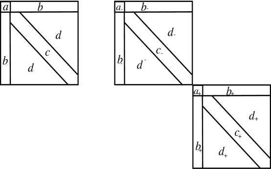
Figure 1. Dividing a symmetric array into four parts.

If $u,v$ are two regions $u,v\in\{a_{\pm},b_{\pm},c_{\pm},d_{\pm}\}$, then by a $u-v$ correlation we mean a correlation between an entry of $A^{0}$ located in the region $u$ and an entry of $A^{0}$ located in the region $v$.

Using (3.8) and (3.9) we deduce that we have

$$\tilde{\sigma}_{1,1}^{0}(\eta)=\frac{-f^{\prime}(0)}{f^{\prime}(0)^{2}-f^{\prime}(r)^{2}-2|\eta|^{2}f^{\prime}(r)f^{\prime\prime}(r)-|\eta|^{4}f^{\prime\prime}(r)^{2}},\;\;V(\xi)=f(|\xi|^{2}/2).$$ (B.2)

The denominator of the above fraction admits a Taylor expansion ($r=\frac{|\eta|^{2}}{2}$)

$$f^{\prime}(0)^{2}-f^{\prime}(r)^{2}-2|\eta|^{2}f^{\prime}(r)f^{\prime\prime}(r)-|\eta|^{4}f^{\prime\prime}(r)^{2}$$

$$=f^{\prime}(0)^{2}-\Biggl{(}\,f^{\prime}(0)+\frac{f^{\prime\prime}(0)|\eta|^{2}}{2}+\frac{f^{\prime\prime\prime}(0)|\eta|^{4}}{8}\,\Biggr{)}^{2}$$

$$-2|\eta|^{2}\Bigl{(}f^{\prime}(0)+\frac{f^{\prime\prime}(0)|\eta|^{2}}{2}\,\Bigr{)}\Bigl{(}f^{\prime\prime}(0)+\frac{f^{\prime\prime\prime}(0)|\eta|^{2}}{2}\Bigr{)}-|\eta|^{4}f^{\prime\prime}(0)^{2}+O(|\eta|^{6})$$

$$=-|\eta|^{2}\Biggl{(}3f^{\prime}(0)f^{\prime\prime}(0)+|\eta|^{2}\Bigl{(}\frac{9}{4}f^{\prime\prime}(0)^{2}+\frac{5}{4}f^{\prime}(0)f^{\prime\prime\prime}(0)\,\Bigr{)}+O(|\eta|^{4})\Biggr{)}$$

Hence

$$\tilde{\sigma}_{1,1}^{0}(\eta)=\frac{1}{3f^{\prime\prime}(0)|\eta|^{2}}\bigl{(}1+c_{1,1}|\eta|^{2}+O(|\eta|^{4})\,\Bigr{)},\;\;c_{1,1}=-\frac{3}{4}\frac{f^{\prime\prime}(0)}{f^{\prime}(0)}-\frac{5}{12}\frac{f^{\prime\prime\prime}(0)}{f^{\prime\prime}(0)}.$$

Next,

$$\tilde{\sigma}_{i,i}^{0}(\eta)=-\frac{f^{\prime}(0)}{f^{\prime}(0)^{2}-f^{\prime}(r)^{2}}$$

$$=-\frac{f^{\prime}(0)}{f^{\prime}(0)^{2}-\Bigl{(}\,f^{\prime}(0)+\frac{f^{\prime\prime}(0)|\eta|^{2}}{2}+\frac{f^{\prime\prime\prime}(0)|\eta|^{4}}{8}\Bigr{)}^{2}+O(|\eta|^{6})}.$$

We conclude that

$$\tilde{\sigma}^{0}_{i,i}(\eta)=\frac{1}{f^{\prime\prime}(0)|\eta|^{2}}\frac{1}{1+\frac{1}{4}\Bigl{(}\frac{f^{\prime\prime\prime}(0)}{f^{\prime\prime}(0)}+\frac{f^{\prime\prime}(0)}{f^{\prime}(0)}\Bigr{)}|\eta|^{2}+O(|\eta|^{4})}$$

$$=\frac{1}{f^{\prime\prime}(0)|\eta|^{2}}\Bigl{(}1+c_{0}|\eta|^{2}+O(|\eta|^{4})\,\Bigr{)},\;\;c_{0}=-\frac{1}{4}\Bigl{(}\frac{f^{\prime\prime\prime}(0)}{f^{\prime\prime}(0)}+\frac{f^{\prime\prime}(0)}{f^{\prime}(0)}\Bigr{)},$$

$$\tilde{\sigma}_{-1,1}^{0}(\eta)=-\frac{f^{\prime}(r)}{f^{\prime}(0)}\tilde{\sigma}^{0}_{1,1}(\eta)$$

$$=-\frac{1}{3f^{\prime\prime}(0)|\eta|^{2}}\Bigl{(}1+c_{1,1}|\eta|^{2}+O(|\eta|^{4})\,\Bigr{)}\Bigl{(}1+\frac{f^{\prime\prime}(0)}{2f^{\prime}(0)}|\eta|^{2}+O(|\eta|^{4})\,\Bigr{)}$$

$$=-\frac{1}{3f^{\prime\prime}(0)|\eta|^{2}}\Bigl{(}1+d_{1,1}|\eta|^{2}+O(|\eta|^{4})\,\Bigr{)},\;\;d_{1,1}=c_{1,1}+\frac{f^{\prime\prime}(0)}{2f^{\prime}(0)},$$

$$\tilde{\sigma}_{-i,i}^{0}(\eta)=-\frac{f^{\prime}(r)}{f^{\prime}(0)}\tilde{\sigma}^{0}_{i,i}$$

$$=-\frac{1}{f^{\prime\prime}(0)|\eta|^{2}}\Bigl{(}1+d_{0}|\eta|^{2}+O(|\eta|^{4})\,\Bigr{)},\;\;d_{0}=c_{0}+\frac{f^{\prime\prime}(0)}{2f^{\prime}(0)}.$$

✩✩✩

$$V_{1,1,1}(\eta)=3|\eta|f^{\prime\prime}(r)+|\eta|^{3}f^{\prime\prime\prime}(r)=|\eta|\Bigl{(}\,3f^{\prime\prime}(0)+\frac{5}{2}|\eta|^{2}f^{\prime\prime\prime}(0)+O(|\eta|^{4})\,\Bigr{)},$$

$$V_{i,i,1}(\eta)=V_{i1i}(\eta)=|\eta|f^{\prime\prime}(r)=|\eta|\Bigl{(}\,f^{\prime\prime}(0)+\frac{1}{2}|\eta|^{2}f^{\prime\prime\prime}(0)+O(|\eta|^{4})\,\Bigr{)},$$

$$V_{11i}(\eta)=0,\;\;i>1,$$

$$V_{i,j,1}(\eta)=0,\;\;j>i>1,$$

$$V_{i,j,k}(\eta)=0,\;\;i,j,k>1.$$

✩✩✩

$$V_{i,j,k,\ell}(0)=\bigl{(}\,\delta_{ij}\delta_{k\ell}+\delta_{ik}\delta_{j\ell}+\delta_{i\ell}\delta_{jk}\,\bigr{)}f^{\prime\prime}(0),$$

$$V_{1,1,1,1}(\eta)=3f^{\prime\prime}(r)+6|\eta|^{2}f^{\prime\prime\prime}(r)+|\eta|^{4}f^{(4)}(r)=3f^{\prime\prime}(0)+\frac{15}{2}f^{\prime\prime\prime}(0)|\eta|^{2}+O(|\eta|^{4}),$$

$$V_{1,1,1,i}(\eta)=0,\;\;i>1,$$

$$V_{1,1,i,i}(\eta)=V_{1,i,1,i}(\eta)=f^{\prime\prime}(r)+|\eta|^{2}f^{\prime\prime\prime}(r)=f^{\prime\prime}(0)+\frac{3}{2}f^{\prime\prime\prime}(0)|\eta|^{2}+O(|\eta|^{4}),\;\;i>1,$$

$$V_{1,1,i,j}(\eta)=V_{1i1j}(\eta)=0,\;\;1<i<j,$$

$$V_{1,i,j,k}(\eta)=0,\;\;i,j,k>1.$$

✶✶

$$V_{i,i,j,j}(\eta)=V_{ijij}(\eta)=f^{\prime\prime}(r),\;\;1<i<j,$$

$$V_{i,i,i,i}(\eta)=3f^{\prime\prime}(r),\;\;i>1,$$

$$V_{i,i,j,k}(\eta)=0,\;\;i>1,\;k>j>1,$$

$$V_{i,j,k,\ell}(\eta)=0,\;\;1<i<j,\;\;1<k<\ell,\;\;(i,j)\neq(k,\ell).$$

✩✩✩

If $1<i<j$, then

$$\bar{\boldsymbol{\Xi}}^{0}_{i,j|k,\ell}(\eta):=V_{i,j,k,\ell}(0),\;\;\bar{\boldsymbol{\Xi}}^{0}_{-i,-j|k,\ell}(\eta):=V_{i,j,k,\ell}(\eta).$$

$\bullet$ $d_{+}-d_{+}$ correlations.

$$\bar{\boldsymbol{\Xi}}^{0}_{i,j|k,\ell}(\eta)=0,\;\;1<k\leq\ell,\;\;(i,j)\neq(k,\ell),$$ (B.3a)

$$\bar{\boldsymbol{\Xi}}^{0}_{i,j|i,j}(\eta)=V_{i,j,i,j}(0)-\sum_{a>0}V_{i,j,a}(\eta)V_{i,j,a}(\eta)\tilde{\sigma}^{0}_{a,a}(\eta)=V_{i,j,i,j}(0)=f^{\prime\prime}(0).$$ (B.3b)

$\bullet$ $c_{+}-c_{+}$ correlations. If $1<i<j$, then

$$\bar{\boldsymbol{\Xi}}^{0}_{i,i|j,j}(\eta)=V_{i,i,j,j}(0)-V_{1,i,i}(\eta)^{2}\tilde{\sigma}_{1,1}^{0}(\eta)=\frac{2}{3}f^{\prime\prime}(0)\Bigl{(}1+O(|\eta|^{2})\Bigr{)},$$ (B.4a)

$$\bar{\boldsymbol{\Xi}}^{0}_{i,i|i,i}(\eta)=V_{i,i,i,i}(0)-V_{1,i,i}(\eta)^{2}\tilde{\sigma}_{1,1}^{0}(\eta)=\frac{8}{3}f^{\prime\prime}(0)\Bigl{(}1+O(|\eta|^{2})\Bigr{)}.$$ (B.4b)

$\bullet$ The $a_{+}-a_{+}$, $a_{+}-b_{+}$, $a_{+}-c_{+}$ and $a_{+}-d_{+}$ correlations. If $1<i<j$, then

$$\bar{\boldsymbol{\Xi}}^{0}_{1,1|1,1}(\eta)=V_{1,1,1,1}(0)-V_{1,1,1}(\eta)^{2}\tilde{\sigma}^{0}_{1,1}(\eta)=\bar{c}_{1,1}|\eta|^{2}\bigl{(}1+O(\eta)^{2}\bigr{)},$$ (B.5a)

$$\bar{c}_{1,1}=-9f^{\prime\prime\prime}(0)-3c_{1,1}f^{\prime\prime}(0),$$ (B.5b)

$$\bar{\boldsymbol{\Xi}}^{0}_{1,1|1,i}(\eta)=0,\;\;i>1,$$ (B.5c)

$$\bar{\boldsymbol{\Xi}}^{0}_{1,1|i,i}(\eta)=V_{1,1,i,i}(0)-V_{1,1,1}(\eta)V_{1,i,i}(\eta)\tilde{\sigma}^{0}_{1,1}(\eta)\sim const.|\eta|^{2},$$ (B.5d)

$$\bar{\boldsymbol{\Xi}}^{0}_{1,1|i,j}(\eta)=0.$$ (B.5e)

$\bullet$ $b_{+}-b_{+}$ correlations. If $1<i<j$, then

$$\bar{\boldsymbol{\Xi}}^{0}_{1,i|1,i}(\eta)=V_{1,i,1,i}(0)-V_{1,i,i}(\eta)^{2}\tilde{\sigma}^{0}_{i,i}(\eta)=\bar{c}_{0}|\eta|^{2}\Bigl{(}1+O(|\eta|^{2})\Bigr{)},$$ (B.6a)

$$\bar{c}_{0}=-f^{\prime\prime\prime}(0)-f^{\prime\prime}(0)c_{0},$$ (B.6b)

$$\bar{\boldsymbol{\Xi}}^{0}_{1,i|1,j}(\eta)=0.$$ (B.6c)

$\bullet$ The $b_{+}-c_{+}$ and $b_{+}-d_{+}$ correllations. If $1<i<j$, then

$$\bar{\boldsymbol{\Xi}}^{0}_{1,i|i,i}(\eta)=V_{1,i,i|i,i}(0)-\sum_{a}V_{1,i,a}(\eta)\tilde{\sigma}_{a,a}^{0}(\eta)V_{a,i,i}(\eta)=0,$$ (B.7a)

$$\bar{\boldsymbol{\Xi}}^{0}_{1,i|j,j}(\eta)=V_{1,i,j,j}(0)-\sum_{a}V_{1,i,a}(\eta)\tilde{\sigma}_{a,a}^{0}(\eta)V_{a,j,j}(\eta)=0,$$ (B.7b)

$$\bar{\boldsymbol{\Xi}}^{0}_{1,i|k,\ell}(\eta)=V_{i,j,k,\ell}(0)-\sum_{a}V_{1,i,a}\tilde{\sigma}_{a,a}^{0}(\eta)V_{a,k,\ell}(\eta)=0,\;\;\forall 1<k<\ell.$$ (B.7c)

$\bullet$ The $a_{-}-a_{+}$, $a_{-}-b_{+}$, $a_{-}-c_{+}$ and $a_{-}-d_{+}$ correlations. If $1<i<j$, then

$$\bar{\boldsymbol{\Xi}}^{0}_{-1,-1|1,1}(\eta)=V_{1,1,1,1}(\eta)+V_{1,1,1}(\eta)^{2}\tilde{\sigma}^{0}_{-1,1}=\bar{d}_{1,1}|\eta|^{2}\Bigl{(}1+O(|\eta|^{2})\Bigr{)},$$ (B.8a)

$$\bar{d}_{1,1}=-3f^{\prime\prime}(0)d_{1,1}-\frac{3}{2}f^{\prime\prime\prime}(0),$$ (B.8b)

$$\bar{\boldsymbol{\Xi}}^{0}_{-1,-1|1,i}(\eta)=0,\;\;i>1,$$ (B.8c)

$$\bar{\boldsymbol{\Xi}}^{0}_{-1,-1|i,i}(\eta)=V_{1,1,i,i}(\eta)+V_{1,1,1}(\eta)V_{1,i,i}(\eta)\tilde{\sigma}^{0}_{-1,1}(\eta)=O(|\eta|^{2}),$$ (B.8d)

$$\bar{\boldsymbol{\Xi}}^{0}_{-1,-1|i,j}(\eta)=V_{1,1,i,j}(\eta)=0,\;\;1<i<j.$$ (B.8e)

$\bullet$ The $b_{-}-b_{+}$, $b_{-}-c_{+}$ and $b_{-}-d_{+}$ correlations.

$$\bar{\boldsymbol{\Xi}}^{0}_{-1,-i|1,i}(\eta)=V_{1,i,1,i}(\eta)+V_{1,i,i}(\eta)^{2}\tilde{\sigma}^{0}_{-i,i}(\eta)=\bar{d}_{0}|\eta|^{2}\Bigl{(}1+O(|\eta|^{2})\,\Bigr{)},$$ (B.9a)

$$\bar{d}_{0}=2f^{\prime\prime\prime}(0)-d_{0}f^{\prime\prime}(0),\;\;i>1,$$ (B.9b)

$$\bar{\boldsymbol{\Xi}}^{0}_{-1,-i|1,j}(\eta)=0,\;\;1<i<j,$$ (B.9c)

$$\bar{\boldsymbol{\Xi}}^{0}_{-1,-i|j,j}(\eta)=0,\;\;i,j>1,$$ (B.9d)

$$\bar{\boldsymbol{\Xi}}^{0}_{-1,-i|j,k}(\eta)=V_{1,i,j,k}(\eta)=0,\;\;1<j<k,\;\;1<i.$$ (B.9e)

$\bullet$ The $c_{-}-c_{+}$ and $c_{-}-d_{+}$ correlations.

$$\bar{\boldsymbol{\Xi}}^{0}_{-i,-i|j,j}(\eta)=V_{i,i,j,j}(\eta)+V_{i,i,1}(\eta)^{2}\tilde{\sigma}^{0}_{-1,1}=\frac{2}{3}f^{\prime\prime}(0)\Bigl{(}1+O(|\eta|^{2})\Bigr{)},\;\;1<i<j,$$ (B.10a)

$$\bar{\boldsymbol{\Xi}}^{0}_{-i,-i|i,i}(\eta)=V_{i,i,i,i}(\eta)+V_{i,i,1}(\eta)^{2}\tilde{\sigma}^{0}_{-1,1}(\eta)=\frac{8}{3}f^{\prime\prime}(0)\Bigl{(}1+O(|\eta|^{2})\Bigr{)},\;\;i>1,$$ (B.10b)

$$\bar{\boldsymbol{\Xi}}^{0}_{-i,-i|j,k}=0,\;\;i>1,k>j>1.$$ (B.10c)

$\bullet$ The $d_{-}-d_{+}$ correlations.

$$\bar{\boldsymbol{\Xi}}^{0}_{-i,-j|i,j}(\eta)=V_{iijj}(\eta)=f^{\prime\prime}(r)=f^{\prime\prime}(0)\Bigl{(}1+O(|\eta|^{2})\Bigr{)},\;\;1<i<j,$$ (B.11a)

$$\bar{\boldsymbol{\Xi}}^{0}_{-i,-j|k,\ell}(\eta)=0,\;\;1<i<j,\;\;1<k<\ell,\;\;(i,j)\neq(k,\ell).$$ (B.11b)

Appendix C Invariant random symmetric matrices

We denote by $\operatorname{\mathbf{Sym}}_{m}$ the space of real symmetric $m\times m$ matrices. The group $O(m)$ acts by conjugation on $\operatorname{\mathbf{Sym}}_{m}$. Would would like to describe the collection $\mathcal{G}_{m}$ of $O(m)$-invariant Gaussian measures on $\mathcal{S}_{n}$.

Observe that $\operatorname{\mathbf{Sym}}_{m}$ is an Euclidean space with respect to the inner product

$$(A,B):=\operatorname{{\rm tr}}(AB).$$ (C.1)

This inner product is invariant with respect to the action of $\operatorname{SO}(m)$ on $\operatorname{\mathbf{Sym}}_{m}$. We set

$$\widehat{\boldsymbol{E}}_{ij}:=\begin{cases}\boldsymbol{E}_{ij},&i=j\\ \frac{1}{\sqrt{2}}E_{ij},&i<j.\end{cases}.$$

The collection $(\widehat{\boldsymbol{E}}_{ij})_{i\leq j}$ is a basis of $\operatorname{\mathbf{Sym}}_{m}$ orthonormal with respect to the above inner product. We defined the normalized entries

$$\hat{a}_{ij}:=\begin{cases}a_{ij},&i=j\\ \sqrt{2}a_{ij},&i<j.\end{cases}$$ (C.2)

The collection $(\hat{a}_{ij})_{i\leq j}$ the orthonormal basis of $\operatorname{\mathbf{Sym}}_{m}^{\vee}{}$ dual to $(\widehat{\boldsymbol{E}}_{ij})$. The volume density induced by this metric is

$$|dA|:=\Bigl{|}\prod_{i\leq j}d\widehat{a}_{ij}\,\Bigr{|}=2^{\frac{1}{2}\binom{m}{2}}\Bigl{|}\,\prod_{i\leq j}da_{ij}\,\Bigr{|}.$$

This volume density is $O(m)$-invariant. Thus, the collection of $O(m)$-invariant Gaussian measures on $\operatorname{\mathbf{Sym}}_{m}$ can be identified with the collection of positive definite $O(m)$-invariant quadratic forms on $\operatorname{\mathbf{Sym}}_{m}$.

The space of $O(m)$-invariant quadratic forms on $\operatorname{\mathbf{Sym}}_{m}$ is two dimensional and spanned by the forms $\operatorname{{\rm tr}}A^{2}$ and $(\operatorname{{\rm tr}}A)^{2}$. For any real numbers $u,v$ such that

$$v>0,mu+2v>0,$$ (C.3)

we denote by $d\boldsymbol{\Gamma}_{u,v}(A)$ the centered Gaussian measure $d\boldsymbol{\Gamma}_{u,v}(A)$ uniquely determined by the covariance equalities

$$\boldsymbol{E}(a_{ij}a_{k\ell})=u\delta_{ij}\delta_{k\ell}+v(\delta_{ik}\delta_{j\ell}+\delta_{i\ell}\delta_{jk}),\;\;\forall 1\leq i,j,.k,\ell\leq m.$$

In particular we have

$$\boldsymbol{E}(a_{ii}^{2})=u+2v,\;\;\boldsymbol{E}(a_{ii}a_{jj})=u,\;\;\;\boldsymbol{E}(a_{ij}^{2})=v,\;\;\forall 1\leq i\neq j\leq m,$$

while all other covariances are trivial. We denote by $\operatorname{\mathbf{Sym}}_{m}^{u,v}$ the space $\operatorname{\mathbf{Sym}}_{m}$ equipped with the probability measure $d\boldsymbol{\Gamma}_{u,v}$ The ensemble $\operatorname{\mathbf{Sym}}_{m}^{0,v}$ is a rescaled version of of the Gaussian Orthogonal Ensemble (GOE) and we will refer to it as $\operatorname{GOE}_{m}^{v}$.

The Gaussian measure $d\boldsymbol{\Gamma}_{u,v}$ coincides with the Gaussian measure $d\boldsymbol{\Gamma}_{u+2v,u,v}$ defined in [10, App. B]. We recall a few facts from [10, App. B].

The probability density $d\boldsymbol{\Gamma}_{u,v}$ has the explicit description

$$d\boldsymbol{\Gamma}_{u,v}(A)=\frac{1}{(2\pi)^{\frac{m(m+1)}{4}}\sqrt{D(u,v)}}e^{-\frac{1}{4v}\operatorname{{\rm tr}}A^{2}-\frac{u^{\prime}}{2}(\operatorname{{\rm tr}}A)^{2}}|dA|,$$ (C.4)

where

$$D(u,v)=(2v)^{(m-1)+\binom{m}{2}}\bigl{(}mu+2v\,\bigr{)},$$

and

$$u^{\prime}=\frac{1}{m}\left(\frac{1}{mu+2v}-\frac{1}{2v}\right)=-\frac{u}{2v(mu+2v)}.$$

This shows that the Gaussian measure $d\Gamma_{u,v}$ is $O(m)$-invariant. Moreover the family $d\boldsymbol{\Gamma}_{u,v}$, where $u,v$ satisfy (C.3) exhausts $\mathcal{G}_{m}$.

For $u>0$ the ensemble $\operatorname{\mathbf{Sym}}_{m}^{u,v}$ can be given an alternate description. More precisely a random $A\in\operatorname{\mathbf{Sym}}_{m}^{u,v}$ can be described as a sum

$$A=B+\ X\mathbbm{1}_{m},\;\;B\in\operatorname{GOE}_{m}^{v},\;\;X\in\boldsymbol{N}(0,u),\;\;\mbox{ $B$ and $X$ independent}.$$

We write this

$$\operatorname{\mathbf{Sym}}_{m}^{u,v}=\operatorname{GOE}_{m}^{v}\hat{+}\boldsymbol{N}(0,u)\mathbbm{1}_{m},$$ (C.5)

where $\hat{+}$ indicates a sum of independent variables.

In the special case $\operatorname{GOE}_{m}^{v}$ we have $u=u^{\prime}=0$ and

$$d\boldsymbol{\Gamma}_{0,v}(A)=\frac{1}{(2\pi v)^{\frac{m(m+1)}{4}}}e^{-\frac{1}{4v}\operatorname{{\rm tr}}A^{2}}|dA|.$$ (C.6)

Fix a unit vector $\eta\in{\mathbb{R}}^{m}$ and denote by $O_{\eta}(m)$ the subgroup of orthogonal map $T:{\mathbb{R}}^{m}\to{\mathbb{R}}^{m}$ such that $T\eta=\eta$. Group $O_{\eta}(m)$ continues to act by conjugation on $\operatorname{\mathbf{Sym}}_{m}$ and we would like to describe the collection $\mathcal{G}_{m,\eta}\supset\mathcal{G}_{m}$ of $O_{\eta}(m)$-invariant Gaussian measures on $\operatorname{\mathbf{Sym}}_{m}$.

The space of $O_{\eta}(m)$-invariant quadratic forms on $\operatorname{\mathbf{Sym}}_{m}$ is five dimensional and it is spanned by the quadratic forms

$$\operatorname{{\rm tr}}A^{2},\;\;(\operatorname{{\rm tr}}A)^{2},\;\;(A^{2}\eta,\eta),\;\;(A\eta,\eta)^{2},\;\;(\operatorname{{\rm tr}}A)(A\eta,\eta).$$

If we choose an orthonormal basis ${\boldsymbol{e}}_{1},\dotsc,{\boldsymbol{e}}_{m}$ of ${\mathbb{R}}^{m}$ such that $\eta={\boldsymbol{e}}_{1}$, then

$$(A\eta,\eta)=a_{11},\;\;(A^{2}\eta,\eta)=\sum_{k=1}^{m}a_{1k}^{2}.$$

If we block decompose a symmetric $m\times m$ matrix

$$A=\left[\begin{array}[]{cc}a_{11}&L^{\dagger}\\ L&B\end{array}\right],$$ (C.7)

where $B\in\mathcal{S}_{m-1}$, $b$ is a $(m-1)\times 1$ matrix, then we see that a basis of the space of $O_{\eta}(m)$-invariant is given by

$$q_{1}(A)=(A\eta,\eta)^{2}=\hat{a}_{11}^{2},$$

$$q_{2}(A)=2|L|^{2}=\sum_{k=2}^{m}\hat{a}_{1k}^{2}=2|A\eta|^{2}-2(A\eta,\eta)^{2},$$

$$q_{3}(A)=2\hat{a}_{11}\operatorname{{\rm tr}}B=2\hat{a}_{11}(\hat{a}_{22}+\cdots+\hat{a}_{mm})=2(A\eta,\eta)\operatorname{{\rm tr}}A-2(A\eta,\eta)^{2},$$

$$q_{4}(A)=(\operatorname{{\rm tr}}B)^{2}=(\hat{a}_{22}+\cdots+\hat{a}_{mm})^{2}=\bigl{(}\,\operatorname{{\rm tr}}A-(A\eta,\eta),\bigr{)}^{2}$$

$$q_{5}(A)=\operatorname{{\rm tr}}B^{2}=\operatorname{{\rm tr}}A^{2}-2|L|^{2}-a_{11}^{2}=\sum_{k=2}^{m}a_{kk}^{2}+\sum_{2\leq i<j}\hat{a}_{ij}^{2}.$$

This suggests dividing a symmetric $m\times m$ array into four regions $a,b,c,d$ as in Figure 2

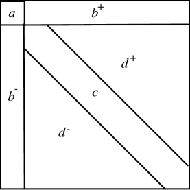
Figure 2. Dividing a symmetric array into four parts.

More precisely, the parts of these regions on or above the diagonal are

$$a=\bigl{\{}\,(1,1)\,\bigr{\}},\;\;b^{+}=\bigl{\{}\,(1,j);\;\;j\geq 2\,\bigr{\}},\;\;c=\bigl{\{}\,(i,i);\;\;i\geq 2\,\bigr{\}},\;\;d^{+}=\bigl{\{}\,(i,j);\;\;i>j\geq 2\,\bigr{\}}.$$

Suppose that $A$ is a Gaussian random symmetric $m\times m$ matrix, where the Gaussian measure is $O_{\eta}(m)$-invariant. Then the entries withing the same region are identically distributed Gaussian variables with variance $v_{a},\dotsc,v_{d}$. Moreover, if we fix regions $r_{1},r_{2}\in\{a,b^{+},c,d^{+}\}$, not necessarily distinct, and $x_{1},x_{2}$ are above or on the diagonal distinct normalized entries, $x_{1}$ in the region $r_{1}$ and $x_{2}$ in the region $r_{2}$, then the covariance $E(x_{1},x_{2})$ is independent of the location of $x_{1}$ and $x_{2}$ in their respective regions, as long as $x_{1}\neq x_{2}$. We denote this covariance $\kappa_{r_{1}r_{2}}$. Thus a $O_{\eta}(m)$-invariant Gaussian measure on $\operatorname{\mathbf{Sym}}_{m}$ is determined by a variance vector

$${\boldsymbol{v}}=(v_{a},v_{b},v_{c},v_{d}),$$

and a symmetric covariance $4\times 4$ matrix

$$K=(\kappa_{r_{1}r_{2}})_{r_{1},r_{2}\in\{a,b,c,d\}}.$$

When representing $K$ as a $4\times 4$ matrix we tacitly assume the order relation $a<b<c<d$.

The quantities ${\boldsymbol{v}}$ and $K$ can be associated to any $O_{\eta}(m)$-invariant quadratic form $q$, whether it is positive semidefinite or not. We denote these quantities ${\boldsymbol{v}}(q)$ and $K(q)$. Observe that

$${\boldsymbol{v}}(xq+x^{\prime}q^{\prime})=x{\boldsymbol{v}}(q)+x^{\prime}{\boldsymbol{v}}(q^{\prime}),\;\;K(xq+x^{\prime}{\boldsymbol{q}}^{\prime})=xK(q)+x^{\prime}K(q^{\prime}),$$

for any real numbers $x,x^{\prime}$ and any $O_{\eta}(m)$-invariant forms $q,q^{\prime}$. Observe that

$${\boldsymbol{v}}(q_{1})=(1,0,0,0),\;K(q_{1})=0,$$

$${\boldsymbol{v}}(q_{2})=(0,1,0,0),\;\;K(q_{2})=\left[\begin{array}[]{cccc}0&0&0&0\\ 0&0&0&0\\ 0&0&0&0\\ 0&0&0&0\end{array}\right],$$

$${\boldsymbol{v}}(q_{3})=(0,0,0,0),\;\;K(q_{3})=\left[\begin{array}[]{cccc}0&0&1&0\\ 0&0&0&0\\ 1&0&0&0\\ 0&0&0&0\end{array}\right],$$

$${\boldsymbol{v}}(q_{4})=(0,0,1,0),\;\;K(q_{4})=\left[\begin{array}[]{cccc}0&0&0&0\\ 0&0&0&0\\ 0&0&1&0\\ 0&0&0&0\end{array}\right],$$

$${\boldsymbol{v}}(q_{5})=(0,0,1,1),\;\;K(q_{5})=0.$$

Thus

$${\boldsymbol{v}}(c_{1}q_{1}+c_{2}q_{2}+c_{3}q_{3}+c_{4}q_{4}+c_{5}q_{5})=(c_{1},c_{2},c_{5}+c_{4},c_{5}),$$

$$K(c_{1}q_{1}+c_{2}q_{2}+c_{3}q_{3}+c_{4}q_{4}+c_{5}q_{5})=\left[\begin{array}[]{cccc}0&0&c_{3}&0\\ 0&0&0&0\\ c_{3}&0&c_{4}&0\\ 0&0&0&0\end{array}\right]$$

We denote by $\operatorname{\mathbf{Sym}}_{m}(c_{1},\dotsc,c_{5})$ the space $\operatorname{\mathbf{Sym}}_{m}$ equipped with the $O_{\eta}(m)$-invariant Gaussian measure with covariance

$$Q_{\vec{c}}:=c_{1}q_{1}+c_{2}q_{2}+c_{3}q_{3}+c_{4}q_{4}+c_{5}q_{5},$$

whenever this quadratic form is positive semidefinite.

For every region $r\in\{a,b,c,d\}$ we denote by $\operatorname{\mathbf{Sym}}_{m}(r)$ the vector subspace of $\operatorname{\mathbf{Sym}}_{m}$ consting of matrices whose entries in regions other than $r$ are trivial. We get an orthogonal direct sum decomposition

$$\operatorname{\mathbf{Sym}}_{m}=\operatorname{\mathbf{Sym}}_{m}(a)\oplus\operatorname{\mathbf{Sym}}_{m}(b)\oplus\operatorname{\mathbf{Sym}}_{m}(c)\oplus\operatorname{\mathbf{Sym}}_{m}(d).$$

This leads to a corresponding decomposition

$$A=A(a)+A(b)+A(c)+A(d),A\in\operatorname{\mathbf{Sym}}_{m}.$$

If $A$ belongs to the ensemble $\operatorname{\mathbf{Sym}}_{m}(c_{1},\dotsc,c_{5})$, then

• the components $A(a),A(b),A(c),A(d)$ are Gaussian vectors,

• the component $A(d)$ is independent of the rest of the other components,

• the $(m-1)\times(m-1)$-random matrix $A(c)+A(d)$ belongs to the ensemble $\operatorname{\mathbf{Sym}}_{m-1}^{c_{4},c_{5}}$.

To decide when $Q_{\vec{c}}\geq 0$ we need to compute the eigenvalues of the the matrix $\mathcal{Q}_{\vec{c}}$ describing $Q_{\vec{c}}$ in the orthonormal coordinates $\hat{a}_{ij}$, $1\leq i\leq j\leq m$.

For any $r\in\{a,b,c,d\}$ denote by $Q(r)$ the matrix representing the restriction of $Q_{\vec{c}}$ to $\operatorname{\mathbf{Sym}}_{m}(r)$. Moreover, for any positive integer $n$, we denote by $C_{n}$ the symmetric $n\times n$ matrix all whose entries are equal to $1$.We have

$$Q(a)=c_{1},\;\;Q(d)=c_{5}\mathbbm{1}_{N},\;\;N=\dim\operatorname{\mathbf{Sym}}_{m-1}(d)=\frac{(m-1)(m-2)}{2},$$

$$Q(b)=c_{2}\mathbbm{1}_{m-1},\;\;Q(c)=c_{5}\mathbbm{1}_{m-1}+c_{4}C_{m-1}$$

Finally, denote by $L_{n}$ the $1\times n$ matrix whose entries are all equal to $1$. With this notation we deduce that $\mathcal{Q}_{\vec{c}}$ has the block decomposition

$$\mathcal{Q}_{\vec{c}}=\left[\begin{array}[]{cccc}Q(a)&c_{2}L_{m-1}&c_{3}L_{m-1}&0\\ c_{2}L_{m-1}^{\dagger}&Q(b)&0&0\\ c_{3}L_{m-1}^{\dagger}&0&Q(c)&0\\ 0&0&0&Q(d)\end{array}\right]=\left[\begin{array}[]{cccc}c_{1}&0&c_{3}L_{m-1}&0\\ 0&c_{2}\mathbbm{1}_{m-1}&0&0\\ c_{3}L_{m-1}^{\dagger}&0&c_{5}\mathbbm{1}_{m-1}+c_{4}C_{m-1}&0\\ 0&0&0&c_{5}\mathbbm{1}_{N}\end{array}\right].$$

To compute the spectrum of $\mathcal{Q}_{\vec{c}}$ it suffices to compute the spectrum of the matrix

$$\left[\begin{array}[]{ccc}c_{1}&0&c_{3}L_{m-1}\\ 0&c_{2}\mathbbm{1}_{m-1}&0\\ c_{3}L_{m-1}^{\dagger}&0&c_{5}\mathbbm{1}_{m-1}+c_{4}C_{m-1}\end{array}\right],$$

viewed as a symmetric operator acting on the space ${\mathbb{R}}\oplus{\mathbb{R}}^{m-1}\oplus{\mathbb{R}}^{m-1}$. We see that the subspace $0\oplus{\mathbb{R}}^{m-1}\oplus 0$ is an invariant subspace of this operator and its restriction to this subspace is $c_{2}\mathbbm{1}_{m-1}$. Thus it suffices to find the spectrum of the operator

$$\bar{\mathcal{Q}}_{\vec{c}}=\left[\begin{array}[]{cc}c_{1}&c_{3}L_{m-1}\\ c_{3}L_{m-1}^{\dagger}&c_{5}\mathbbm{1}_{m-1}+c_{4}C_{m-1}\end{array}\right]$$

acting on $\boldsymbol{V}={\mathbb{R}}\oplus{\mathbb{R}}^{m-1}$. A vector ${\boldsymbol{v}}\in\boldsymbol{V}$ has a decomposition

$${\boldsymbol{v}}=\left[\begin{array}[]{c}t\\ {\boldsymbol{x}}\end{array}\right],\;\;{\boldsymbol{x}}=\left[\begin{array}[]{c}x_{1}\\ \vdots\\ x_{m-1}\end{array}\right].$$

We set

$${\sigma}({\boldsymbol{x}})=x_{1}+\cdots+x_{m-1},\;\;{\mathbf{u}}=L_{m-1}^{\dagger}=\left[\begin{array}[]{c}1\\ \vdots\\ 1\end{array}\right]\in{\mathbb{R}}^{m-1}.$$

We have

$$\bar{\mathcal{Q}}_{\vec{c}}\left[\begin{array}[]{c}t\\ {\boldsymbol{x}}\end{array}\right]=\left[\begin{array}[]{c}c_{1}t+c_{3}{\sigma}({\boldsymbol{x}})\\ c_{3}t{\mathbf{u}}+c_{5}{\boldsymbol{x}}+c_{4}{\sigma}({\boldsymbol{x}}){\mathbf{u}}.\end{array}\right].$$ (C.8)

This shows that the codimension $2$ subspace $\boldsymbol{V}_{0}\subset\boldsymbol{V}$ given by

$$t=0,\;\;{\sigma}({\boldsymbol{x}})=0,$$

is $\bar{\mathcal{Q}}_{\vec{c}}$-invariant, and the restriction of $\bar{\mathcal{Q}}_{\vec{c}}$ to this subspace is $c_{5}\mathbbm{1}_{\boldsymbol{V}_{0}}$.

An orthogonal basis of the orthogonal complement $\boldsymbol{W}_{0}:=\boldsymbol{V}_{0}^{\perp}$ is given by the vectors

$${\boldsymbol{v}}_{0}=\left[\begin{array}[]{c}1\\ 0\end{array}\right],\;\;{\boldsymbol{v}}_{1}=\left[\begin{array}[]{c}0\\ {\mathbf{u}}\end{array}\right].$$

Using (C.8) we deduce

$$\bar{\mathcal{Q}}_{\vec{c}}(t_{0}{\boldsymbol{v}}_{0}+t_{1}{\boldsymbol{v}}_{1})=\bigl{(}\,c_{1}t_{0}+(m-1)c_{3}t_{1}\,\bigr{)}{\boldsymbol{v}}_{0}$$

$$+\bigr{(}\,c_{2}t_{0}+c_{5}t_{1}\bigl{)}{\boldsymbol{v}}_{1}+\bigl{(}\,c_{3}t_{0}+(c_{5}+(m-1)c_{4})t_{2}\,\bigr{)}{\boldsymbol{v}}_{2}.$$

Thus in the basis ${\boldsymbol{v}}_{0},{\boldsymbol{v}}_{1},{\boldsymbol{v}}_{2}$ of $V_{0}^{\perp}$ the restriction of $\bar{\mathcal{Q}}_{\vec{c}}$ to this subspace is given by the $2\times 2$ matrix

$$\Sigma_{\vec{c}}=\left[\begin{array}[]{ccc}c_{1}&(m-1)c_{3}\\ c_{3}&c_{5}+(m-1)c_{4}\end{array}\right].$$

Putting together all the above facts we obtain the following result.

Proposition C.1.

The quadratic form $Q_{\vec{c}}$ is positive definite if and only if $c_{1},c_{2},c_{5}>0$ and $\det\Sigma_{\vec{c}}>0$. Moreover

$$\det Q_{\vec{c}}=\Delta(\vec{c})=c_{2}^{m-1}c_{5}^{N+\dim\boldsymbol{V}_{0}}\det\Sigma_{\vec{c}}=c_{2}^{m-1}c_{5}^{\frac{(m-1)(m-2)}{2}+m-2}\det\Sigma_{\vec{c}}.$$ (C.9)

$\hbox to0.0pt{$\sqcap$\hss}\sqcup$

Remark C.2.

(a) The matrix $\Sigma_{\vec{c}}$ is similar to the symmetric matrix

$$\hat{\Sigma}_{\vec{c}}=\left[\begin{array}[]{ccc}c_{1}&(m-1)^{\frac{1}{2}}c_{3}\\ (m-1)^{\frac{1}{2}}c_{3}&c_{5}+(m-1)c_{4}\end{array}\right].$$

Thus $\mathcal{Q}_{\vec{c}}$ is positive definite iff $c_{2},c_{5}>0$ and the symmetric matrix $\hat{\Sigma}_{\vec{c}}$ is positive definite.

(b) The above proof produced an orthogonal decomposition of $\operatorname{\mathbf{Sym}}_{m}$

$$\operatorname{\mathbf{Sym}}_{m}=\operatorname{\mathbf{Sym}}_{m}(d)\oplus\operatorname{\mathbf{Sym}}_{m}(b)\oplus\boldsymbol{V},\;\;\boldsymbol{V}=\operatorname{\mathbf{Sym}}_{m}(a)\oplus\operatorname{\mathbf{Sym}}_{m}(c).$$

In the proof we used the natural metric (C.1) on $\operatorname{\mathbf{Sym}}_{m}$ to identify $Q_{\vec{c}}$ with a symmetric operator $\operatorname{\mathbf{Sym}}_{m}\to\operatorname{\mathbf{Sym}}_{m}$. The three factors above are invariant subspaces of this operator. The restriction of $Q_{\vec{c}}$ to $\operatorname{\mathbf{Sym}}_{m}(d)$ is $c_{5}\mathbbm{1}$, while the restriction of $Q_{\vec{c}}$ to $\operatorname{\mathbf{Sym}}_{m}(b)$ is $c_{2}\mathbbm{1}$. The subspace $\boldsymbol{V}$ decomposes further into two invariant subspaces: the two-dimensional subspace

$$\boldsymbol{W}_{0}=\operatorname{\mathbf{Sym}}_{m}(a)\oplus\operatorname{span}\mathbbm{1}_{m-1}={\mathbb{R}}\oplus\operatorname{span}{\mathbbm{1}}_{m-1},\;\;\mathbbm{1}_{m-1}\in\operatorname{\mathbf{Sym}}_{m}(c),$$

and its orthogonal complement $\boldsymbol{V}_{0}$. The restriction of $Q_{\vec{c}}$ to $\boldsymbol{V}_{0}$ is $c_{5}\mathbbm{1}_{\boldsymbol{V}_{0}}$ while the restriction to $\boldsymbol{W}_{0}$ is described in the canonical orthonormal basis

$$1\oplus 0,\;\;0\oplus\frac{1}{\sqrt{m-1}}\mathbbm{1}_{m-1}$$

by the matrix $\hat{\Sigma}_{\vec{c}}$.

(c) We denote by $\mathcal{T}_{\eta}$ the space of $O_{\eta}(m)$-equivariant symmetric operators

$$T:\operatorname{\mathbf{Sym}}_{m}\to\operatorname{\mathbf{Sym}}_{m}$$

The above discussion shows that any $T\in\mathcal{T}_{\eta}$ enjoys the following properties.

• Each of the subspaces $\operatorname{\mathbf{Sym}}_{m}(d)$, $\operatorname{\mathbf{Sym}}_{m}(b)$, $\boldsymbol{V}_{0}$ and $\boldsymbol{W}_{0}$ are $T$-invariant, where $\boldsymbol{V}_{0}$ and $\boldsymbol{W}_{0}$ are defined as in (b).

• There exist two real constants $\alpha,\beta$ such that the restriction of $T$ to $\operatorname{\mathbf{Sym}}_{m}(b)$ is $\alpha\mathbbm{1}$, while the restriction of $T$ to $\operatorname{\mathbf{Sym}}_{m}(d)\oplus\boldsymbol{V}_{0}$ is $\beta\mathbbm{1}$. ($\alpha=c_{2}$, $\beta=c_{5}$.)

We denote by $\hat{\Sigma}_{T}$ the restriction of $T$ to $\boldsymbol{W}_{0}$. We see that an operator $T\in\mathcal{T}_{\eta}$ is determined by a triplet $(\alpha,\beta,S)$ where $\alpha,\beta\in{\mathbb{R}}$ and $S:\boldsymbol{W}_{0}\to\boldsymbol{W}_{0}$ is a symmetric operator. We will denote by $T_{\alpha,\beta,S}$ the operator associated to this triplet. Note also that $T_{\alpha,\beta,S}$ is invertible iff $\alpha\beta\det S\neq 0$ and

$$T_{\alpha,\beta,S}^{-1}=T_{\alpha^{-1},\beta^{-1},S^{-1}}.$$

A matrix $A\in\operatorname{\mathbf{Sym}}_{m}$ has the block form (C.7)

$$A=\left[\begin{array}[]{cc}a_{11}&L^{\dagger}\\ L&B\end{array}\right]$$

we further decompose $B$ as a sum

$$B:=\frac{c}{\sqrt{m-1}}\mathbbm{1}_{m-1}+B_{0},\;\;\operatorname{{\rm tr}}B_{0}=0,$$

so that $c\sqrt{m-1}=\operatorname{{\rm tr}}B$. We we will refer to this matrix using the notation $A=A(a_{11},L,c,B_{0})$. Then

$$T_{a,b,S}A(a_{11},L,c,B_{0})=A(a_{11}^{\prime},L^{\prime},c^{\prime},B_{0}^{\prime}),$$

where

$$B_{0}^{\prime}=\beta B_{0},\;\;L^{\prime}=\alpha L,\;\;\left[\begin{array}[]{cc}a_{11}^{\prime}\\ c^{\prime}\end{array}\right]=S\left[\begin{array}[]{cc}a_{11}\\ c\end{array}\right]. \hbox to0.0pt{$\sqcap$\hss}\sqcup$$

References

- [1] R. Adler, R.J.E. Taylor: Random Fields and Geometry, Springer Monographs in Mathematics, Springer Verlag, 2007.
- [2] J.-M. Azaïs, M. Wschebor: Level Sets and Extrema of Random Processes, John Wiley & Sons, 2009.
- [3] P.M. Bleher, Y. Homma, R.K.W. Roeder: Two-point correlation functions and universality for systems of -invariant Gaussian random polynomials, arXiv: 1502.01427.
- [4] A. Granville, I. Wigman: The distribution of zeroes of random trigonometric polynomials, Amer. J. Math. 133(2011), 295-357. arXiv: 0809.1848.
- [5] I.M. Gelfand, N.Ya. Vilenkin: Generalized Functions, vol. 4, Academic Press, New York, 1964.
- [6] L. Hörmander: The Analysis of Linear Partial Differential Operators I., Springer Verlag, 2003.
- [7] M. Krishnapur, P. Kurlberg, I. Wigman: Nodal length fluctuations for arithmetic random waves, arXiv: 1111.2800, Ann. Math., 177(2013), 699-737.
- [8] L.I. Nicolaescu: Lectures on the Geometry of Manifolds, 2nd Edition, World Scientific, 2007.
- [9] L.I. Nicolaescu: Fluctuations of the number of critical points of random trigonometric polynomials, An. Sti. Univ. Iasi, vol. 54, f1, (2013), 1-24.
- [10] L.I. Nicolaescu: Critical sets of random smooth functions on compact manifolds, arXiv: 1101.5990, to appear in Asian J. Math
- [11] L.I. Nicolaescu: Random Morse functions and spectral geometry, arXiv: 1209.0639.
- [12] Z. Rudnick, I. Wigman: On the volume of nodal sets for eigenfunctions of the Laplacian on the torus, arXiv: math-ph/0702081, Ann. Henri Poincaré, 9(2008), 109-130.
- [13] B. Shiffman, S. Zelditch: Number variance of random zeros on complex manifolds, arXiv: math/0608743, GAFA, 8(2008), 1422-1475.
- [14] B. Shiffman, S. Zelditch: Number variance of random zeros on complex manifolds, II: smooth statistics, arXiv: 0711.1840, Pure Appl. Math. Q. 6(2010), no.4, Special Issue: In honor of Joseph J. Kohn. Part 2, 1145-1167.
- [15] E. Subag: The complexity of spherical -spin models: a second moment approach, arXiv: 1504.02251.
- [16] I. Wigman: On the distribution of the nodal sets of random spherical harmonics, arXiv: 0805.2768, J. Math. Phys. 50, 013521, 2009.
- [17] I. Wigman: Fluctuations of the nodal length of random spherical harmonics, arXiv: 0907.1648, Comm. Math. Phys., 298(2010), 787-831.